1. Introduction
When nonlinear internal waves interact with the continental or nearshore slope, they shoal and break, generating cross-shelf velocities throughout the water column. Observations have shown that these flows affect the transport of physically and biologically important scalars such as temperature (Leichter et al. Reference Leichter, Wing, Miller and Denny1996; Davis & Monismith Reference Davis and Monismith2011; Walter et al. Reference Walter, Woodson, Arthur, Fringer and Monismith2012), nutrients (Leichter et al. Reference Leichter, Wing, Miller and Denny1996; Omand et al. Reference Omand, Leichter, Franks, Guza, Lucas and Feddersen2011), sediments (Bogucki, Dickey & Redekopp Reference Bogucki, Dickey and Redekopp1997; Klymak & Moum Reference Klymak and Moum2003; Hosegood, Bonnin & van Haren Reference Hosegood, Bonnin and van Haren2004; Hosegood & van Haren Reference Hosegood and van Haren2004; Carter, Gregg & Lien Reference Carter, Gregg and Lien2005; Quaresma et al. Reference Quaresma, Vitorino, Oliveira and da Silva2007), larvae (Pineda Reference Pineda1994) and dissolved oxygen (Walter et al. Reference Walter, Woodson, Leary and Monismith2014). Due to the difficulty in capturing internal wave breaking events with adequate spatial and temporal resolution in the field, laboratory experiments and numerical simulations have been used widely to investigate internal wave breaking dynamics. Such studies have focused on the kinematics of wave breaking (Wallace & Wilkinson Reference Wallace and Wilkinson1988; Helfrich Reference Helfrich1992; Vlasenko & Hutter Reference Vlasenko and Hutter2002; Venayagamoorthy & Fringer Reference Venayagamoorthy and Fringer2007), classifying breaker types (Boegman, Ivey & Imberger Reference Boegman, Ivey and Imberger2005; Aghsaee, Boegman & Lamb Reference Aghsaee, Boegman and Lamb2010), wave reflection (Bourgault & Kelley Reference Bourgault and Kelley2007; Aghsaee et al. Reference Aghsaee, Boegman and Lamb2010) and quantifying turbulence and mixing (Michallet & Ivey Reference Michallet and Ivey1999; Boegman et al. Reference Boegman, Ivey and Imberger2005; Arthur & Fringer Reference Arthur and Fringer2014). However, only a few laboratory or numerical studies have addressed transport due to breaking internal waves on slopes (Helfrich Reference Helfrich1992; Bourgault, Kelley & Galbraith Reference Bourgault, Kelley and Galbraith2005; Nakayama & Imberger Reference Nakayama and Imberger2010; Nakayama et al. Reference Nakayama, Shintani, Kokubo, Kakinuma, Maruya, Komai and Okada2012; Bourgault et al. Reference Bourgault, Morsilli, Richards, Neumeier and Kelley2014).
Before breaking occurs, internal waves propagating over a flat bottom are known to transport mass. This phenomenon was first observed in the field by Shanks (Reference Shanks1983), but was examined more thoroughly by Lamb (Reference Lamb1997) for internal solitary waves. Lamb (Reference Lamb1997) showed that for an approximately two-layer stratification (two well-mixed layers separated by a sharp pycnocline), transport occurs in the direction of wave propagation in the upper layer and in the opposite direction in the lower layer. Transport increases with wave amplitude and is maximized at the surface.
As internal waves interact with a sloping bottom, the associated transport is affected by the breaking process. Using dye as a tracer in laboratory experiments on breaking internal waves on slopes, Helfrich (Reference Helfrich1992) showed that onshore transport occurs as dense fluid flows upslope as a bore or bolus after breaking. In addition, Nakayama & Imberger (Reference Nakayama and Imberger2010) and Nakayama et al. (Reference Nakayama, Shintani, Kokubo, Kakinuma, Maruya, Komai and Okada2012) used a combination of laboratory measurements and numerical modelling to quantify transport using a time-averaged residual circulation. This circulation describes transport that is generally onshore in the upper layer and offshore in the lower layer. Several laboratory (Ivey & Nokes Reference Ivey and Nokes1989; Helfrich Reference Helfrich1992; McPhee-Shaw & Kunze Reference McPhee-Shaw and Kunze2002; Nakayama & Imberger Reference Nakayama and Imberger2010) and numerical (Bourgault et al. Reference Bourgault, Kelley and Galbraith2005, Reference Bourgault, Morsilli, Richards, Neumeier and Kelley2014; Nakayama & Imberger Reference Nakayama and Imberger2010) studies have shown that breaking internal waves on slopes drive offshore transport along the pycnocline due to intrusions of mixed fluid after breaking. These intrusions resemble intermediate nepheloid layers (INLs), a common feature of the coastal ocean. Intermediate nepheloid layers have been observed to spread offshore along isopycnals from mixing regions associated with internal wave breaking on slopes in the field (McPhee-Shaw et al. Reference McPhee-Shaw, Sternberg, Mullenbach and Ogston2004; McPhee-Shaw Reference McPhee-Shaw2006; Cheriton et al. Reference Cheriton, McPhee-Shaw, Shaw, Stanton, Bellingham and Storlazzi2014), and can transport benthic material into the interior of the water column of the order of 1–10 km offshore (McPhee-Shaw Reference McPhee-Shaw2006).
Mass transport has also been studied for shoaling internal solitary waves of depression. Lamb (Reference Lamb2002, Reference Lamb2003) investigated the formation of ‘trapped cores’ of dense fluid within shoaling internal solitary waves of depression using a numerical model. Trapped cores have been observed in the field, for example in the South China Sea within shoaling internal solitary waves of depression (Lien et al. Reference Lien, D’Asaro, Henyey, Chang, Tang and Yang2012, Reference Lien, Henyey, Ma and Yang2014). For a particular wave, Lien et al. (Reference Lien, D’Asaro, Henyey, Chang, Tang and Yang2012) gave an instantaneous estimate of mass transport within the trapped core of 18 Sv, and an average estimate of 0.05 Sv per day. Trapped cores have also been observed in internal solitary waves of elevation in the field, and it has been suggested that they provide a mechanism for the transport of benthic material and nutrients associated with cold dense water in the ocean (Klymak & Moum Reference Klymak and Moum2003; Scotti & Pineda Reference Scotti and Pineda2004).
In this study, high-resolution numerical simulations are used in conjunction with a particle-tracking model to investigate transport due to breaking internal gravity waves on slopes. Section 2 summarizes the computational set-up, which is based on that of Arthur & Fringer (Reference Arthur and Fringer2014). Using the results of a three-dimensional direct numerical simulation (DNS), § 3 describes cross-shore transport, while § 4 explores the effects of three-dimensional dynamics on transport. Then, § 5 considers several applications of two-dimensional simulations, including the variation of cross-shore transport with wave amplitude and bathymetric slope, as well as the composition of INLs.
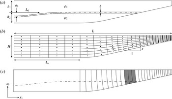
The domain used to study breaking internal gravity waves on slopes. Here, (
 $x_{1},x_{2},x_{3}$
) are Cartesian coordinates in the cross-shore, lateral (along-shore, into the page) and vertical directions respectively. (a) The initial stratification, where
 ${\it\rho}_{1}=985~\text{kg}~\text{m}^{-3}$
,
 ${\it\rho}_{2}=1015~\text{kg}~\text{m}^{-3}$
(
 ${\rm\Delta}{\it\rho}=30~\text{kg}~\text{m}^{-3}$
) and
 ${\it\delta}=2~\text{cm}$
. The parameters
 $a_{0}$
,
 $L_{w}$
,
 $h_{1}$
and
 $h_{2}$
are shown in table 1. (b) The physical dimensions of the domain and a coarse example of the orthogonal curvilinear grid (without vertical stretching). The parameters
 $L$
,
 $H$
and
 $s$
are shown in table 1. In three-dimensional cases, the lateral (
 $x_{2}$
) width of the domain is
 $W=0.1~\text{m}$
. The radius of curvature of the rounded bottom at the beginning of the slope is 3 m, and
 $L_{s}=1.675~\text{m}$
for all cases. (c) A coarse example of the particle initialization for cases 3t1 and 1–7. Vertical lines indicate particles at each vertical grid point and every 10 horizontal grid points. Grey shading represents a particle plume just offshore of the intersection of the initial pycnocline and the slope, as shown in figure 4.

2. Computational approach
2.1. Computational set-up
We simulate breaking internal gravity waves on slopes in an idealized laboratory-scale domain using the parallel Navier–Stokes code of Cui (Reference Cui1999) on a curvilinear grid. This code employs the method of Zang, Street & Koseff (Reference Zang, Street and Koseff1994), which has been used extensively in the past to study geophysical flows at the laboratory scale (see Venayagamoorthy & Fringer Reference Venayagamoorthy and Fringer2007; Chou & Fringer Reference Chou and Fringer2010; Arthur & Fringer Reference Arthur and Fringer2014). The computational set-up used here is based on that of Arthur & Fringer (Reference Arthur and Fringer2014) and is summarized in figure 1(a,b). Simulations were run on the US Army Research Laboratory DoD Supercomputing Research Center (ARL DSRC) supercomputers Pershing and Excalibur.
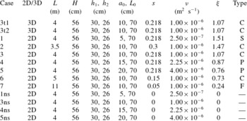
The wave cases considered in this study in terms of the dimensionality of the simulation, the domain length
 $L$
, the domain height
 $H$
, the upper-layer depth
 $h_{1}$
, the lower-layer depth
 $h_{2}$
, the amplitude of the initial half-Gaussian
 $a_{0}$
, the length scale of the initial half-Gaussian
 $L_{0}$
, the bottom slope
 $s$
, the kinematic viscosity
 ${\it\nu}$
, the internal Iribarren number
 ${\it\xi}$
and the breaker type (S
 $=$
surging, C
 $=$
collapsing, P
 $=$
plunging, F
 $=$
fission).

We focus our results in §§ 3 and 4 on breaking wave case 3t1, a three-dimensional DNS case that is summarized in table 1. An additional three-dimensional DNS case, case 3t2, which has the same physical set-up as case 3t1 but a different particle configuration (see § 2.3), is considered in § 5.1. Seven two-dimensional (
 $x_{1}$
,
 $x_{3}$
) cases are considered in §§ 5.2 and 5.3. These cases are two-dimensional versions of cases 1–7 in Arthur & Fringer (Reference Arthur and Fringer2014), and include four cases with constant bathymetric slope
 $s$
and varying initial wave amplitude
 $a$
(cases 1, 3, 4, 5), as well as four cases with constant initial amplitude
 $a$
and varying slope
 $s$
(cases 2, 3, 6, 7). The initial wave amplitude
 $a$
is measured once it has formed from the initial condition, and is approximately
 $a_{0}/2$
(see § 2.2). A constant wave Reynolds number
 $Re_{w}=a^{2}{\it\omega}_{0}/{\it\nu}\approx 208$
, where the wave frequency
 ${\it\omega}_{0}=c_{0}/{\it\lambda}$
, is maintained by changing the molecular viscosity
 ${\it\nu}$
(Arthur & Fringer Reference Arthur and Fringer2014). Here, we estimate the wave speed as the linear phase speed in a two-layer system,
 $c_{0}=\sqrt{g^{\prime }h_{1}h_{2}/H}=0.20~\text{m}~\text{s}^{-1}$
. The wavelength is approximated by
 ${\it\lambda}=2L_{w}$
(Michallet & Ivey Reference Michallet and Ivey1999; Arthur & Fringer Reference Arthur and Fringer2014). The wave length scale
 $L_{w}=1/a\int _{0}^{L_{s}}{\it\eta}(x_{1})\,\text{d}x_{1}\approx 1.2~\text{m}$
for all cases, where
 ${\it\eta}$
is the displacement of the
 ${\it\rho}={\it\rho}_{0}$
isopycnal from
 $h_{1}$
(Michallet & Ivey Reference Michallet and Ivey1999). The Prandtl number
 $Pr=1$
such that the molecular diffusivity
 ${\it\kappa}={\it\nu}$
. Case 3 is considered to be the base case with
 ${\it\nu}=10^{-6}~\text{m}^{2}~\text{s}^{-1}$
. Finally, four two-dimensional cases with no slope (cases 1ns, 3ns, 4ns, 5ns) are included for comparison with cases 1, 3, 4 and 5, and are discussed in § 5.2.
Computations are made on an orthogonal curvilinear grid generated with the open-source software gridgen (available online at https://code.google.com/p/gridgen-c/). Three-dimensional cases (cases 3t1 and 3t2) are computed on a grid of size
 $N_{1}\times N_{2}\times N_{3}=1152\times 96\times 128\approx 14\times 10^{6}$
grid points. Grid stretching of the form
 ${\rm\Delta}x_{i}^{k}=r{\rm\Delta}x_{i}^{k+1}$
, where
 $r$
is the stretching factor and
 $k$
is the index of the grid point, is employed in the horizontal (
 $x_{1}$
) and vertical (
 $x_{3}$
) directions to increase the resolution in the breaking region. In the horizontal direction, stretching is applied from
 $x_{1}=0$
to
 $L_{s}$
with
 $r=1.01$
, concentrating approximately 90 % of the grid points into the sloping region. The grid is also stretched slightly in
 $x_{1}$
in the sloping region to maintain orthogonality. In the vertical direction, stretching is performed twice. First, grid points are concentrated towards the bottom with
 $r=1.02$
in order to resolve the flow near the wall. Second, 100 of 128 points (78 %) are concentrated in the bottom 35 % of the domain with
 $r=1.07$
in order to resolve the pycnocline and lower layer during breaking. The resulting grid resolution at the pycnocline in the breaking region is approximately
 ${\rm\Delta}x_{1}\times {\rm\Delta}x_{2}\times {\rm\Delta}x_{3}=4\times 1\times 2~\text{mm}$
. Near the bottom wall, the vertical coordinate is measured in wall units
 $x_{3}^{+}=x_{3}/{\it\delta}_{S}$
, where the Stokes layer thickness is given by
 ${\it\delta}_{s}=\sqrt{2{\it\nu}/{\it\omega}_{0}}$
. The vertical resolution near the wall is therefore
 ${\rm\Delta}x_{3}^{+}={\rm\Delta}x_{3}/{\it\delta}_{S}<1$
. The grid spacing in the lateral (
 $x_{2}$
) direction is constant. In the worst-case scenario, the grid spacing in cases 3t1 and 3t2 is found to be within approximately one order of magnitude of the Kolmogorov length scale
 ${\it\eta}_{k}$
, providing sufficient resolution for DNS (see Arthur & Fringer Reference Arthur and Fringer2014). The two-dimensional cases 1, 3, 4, and 5 are computed on a grid of size
 $N_{1}\times N_{3}=1152\times 128$
. To account for different length domains,
 $N_{1}=1024$
for case 2,
 $N_{1}=1408$
for case 6 and
 $N_{1}=2048$
for case 7. The boundary conditions for all velocity components are no-slip on the bottom wall and free-slip on the top, left and right walls. The density field has a gradient-free boundary condition on the top, bottom, left and right walls. All variables are periodic in the lateral direction. A time step of
 ${\rm\Delta}t=0.003~\text{s}$
is used for all cases, and the wave period
 $T=2{\rm\pi}/{\it\omega}_{0}\approx 76~\text{s}$
is used to normalize
 $t$
in all figures.
2.2. Incoming wave properties
The stratification in each breaking wave case is initialized as
 $$\begin{eqnarray}\frac{{\it\rho}}{{\it\rho}_{0}}(x_{1},x_{3},t=0)=1-\frac{{\rm\Delta}{\it\rho}}{2{\it\rho}_{0}}\tanh \left[\frac{2(x_{3}+h_{1}+{\it\zeta}(x_{1}))}{{\it\delta}}\tanh ^{-1}({\it\alpha})\right],\end{eqnarray}$$
where the reference density
 ${\it\rho}_{0}=1000~\text{kg}~\text{m}^{-3}$
, the density difference between the top and bottom layers
 ${\rm\Delta}{\it\rho}={\it\rho}_{2}-{\it\rho}_{1}=30~\text{kg}~\text{m}^{-3}$
, the upper-layer depth
 $h_{1}=0.3~\text{m}$
, the interface thickness
 ${\it\delta}=2~\text{cm}$
and
 ${\it\alpha}=0.99$
. The incoming wave is created in our simulations by initializing a half-Gaussian depression in the density interface at the left boundary (Fringer Reference Fringer2003; Bourgault & Kelley Reference Bourgault and Kelley2007). Thus,
 $$\begin{eqnarray}{\it\zeta}(x_{1})=a_{0}\exp \left[-\!\left(\frac{x_{1}}{L_{0}}\right)^{2}\right]+{\it\zeta}^{\prime }R,\end{eqnarray}$$
where
 $a_{0}$
and
 $L_{0}$
are the initial amplitude and length scale of the half-Gaussian respectively, as shown in table 1. An initial perturbation
 ${\it\zeta}^{\prime }R$
, where
 ${\it\zeta}^{\prime }=1$
mm and
 $R\in \{-1,1\}$
is a uniformly distributed random number, is also added to the interface to trigger lateral instabilities during breaking in the three-dimensional simulations (cases 3t1 and 3t2).
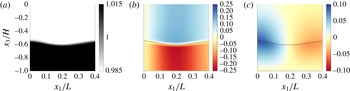
Once the simulation starts, the half-Gaussian depression forms an internal wave of depression that propagates towards the slope. The density and velocity fields of the wave once it has formed (
 $t/T=0.07$
) are shown in figure 2 for case 3t1. It should be noted that the amplitude of the incoming wave
 $a$
is estimated at this time. The velocity fields in figure 2(b,c) are normalized by the linear wave speed
 $c_{0}$
, which is found to be a good estimate of the actual wave propagation speed for all cases. The initial wave shown in figure 2 for case 3t1, as well as those in all other cases, resembles an internal solitary wave. However, we note that the properties of internal solitary waves, including wave amplitude, wavelength and wave speed, are dependent on a specified wave energy within a given background stratification and shear field. This relationship is governed by the nonlinear Dubreil-Jacotin–Long (DJL) equation (see Lamb Reference Lamb2002, and references therein). Due to the potential differences between the initial waves in our simulations and true internal solitary waves that satisfy the DJL equation, we refer to the waves in this study more generally as internal gravity waves.
The density and velocity fields of the incoming wave after it has formed from the initial half-Gaussian (
 $t/T=0.07$
) for case 3t1: (a) the density field
 ${\it\rho}/{\it\rho}_{0}$
, (b) the horizontal velocity field
 $u_{1}/c_{0}$
and (c) the vertical velocity field
 $u_{3}/c_{0}$
. The velocities
 $u_{1}$
and
 $u_{3}$
are both normalized by the linear wave speed in a two-layer system,
 $c_{0}$
.

The decision to initialize the present wave cases with a half-Gaussian at the interface instead of a DJL internal solitary wave was made due to computational restrictions associated with the three-dimensional DNS cases. As described in the review of Helfrich & Melville (Reference Helfrich and Melville2006), an internal solitary wave is a wave of depression when
 $h_{1}<h_{2}$
. Then, as it shoals and
 $h_{1}>h_{2}$
, the polarity of the wave changes and it becomes a wave of elevation. Thus, a relatively large
 $h_{2}$
is required for a true internal solitary wave of depression, which requires a deeper (and therefore longer) domain. By using an initial half-Gaussian, we were able to bypass this restriction and create waves of depression with
 $h_{1}>h_{2}$
, allowing us to achieve the resolution required for DNS. If
 $h_{1}<h_{2}$
, a wave initialized with a half-Gaussian can become an internal solitary wave, assuming that it has enough time to evolve before hitting the slope. This was the case in Bourgault et al. (Reference Bourgault, Kelley and Galbraith2005) and Bourgault & Kelley (Reference Bourgault and Kelley2007), where a two-dimensional numerical model was used to study breaking internal solitary waves on slopes, as well as in Helfrich (Reference Helfrich1992) and Michallet & Ivey (Reference Michallet and Ivey1999), where breaking internal waves on slopes were studied in the laboratory. Instead, we chose to minimize the propagation distance and time prior to the interaction of the wave with the slope in order to focus computational effort on wave breaking.
2.3. Particle tracking
In order to quantify transport by internal gravity waves as they shoal and break on a slope, particle tracking is included in the computations. The use of particle tracking in this study has several benefits over passive scalars, which have been used in the past to examine transport by breaking internal waves on slopes numerically (Bourgault et al. Reference Bourgault, Kelley and Galbraith2005; Nakayama & Imberger Reference Nakayama and Imberger2010). Unlike a passive scalar, particle motion is not affected by numerical diffusion. Furthermore, we are able to investigate transport as a function of the initial position of individual particles, rather than the initial distribution of a scalar. The particle-tracking code used here is based on the code of Gil & Fringer (Reference Gil and Fringer2015), who studied particle drift in nonlinear internal gravity waves. The motion of the particles is governed by
 $$\begin{eqnarray}\frac{\text{d}x_{i}^{\,p}}{\text{d}t}=u_{i}^{p},\end{eqnarray}$$
where
 $x_{i}^{\,p}$
and
 $u_{i}^{p}$
are the position and velocity of particle
 $p$
in the
 $i$
th Cartesian coordinate direction (
 $i=1,2,3$
) respectively. Equation (2.3) is solved using a fourth-order Runge–Kutta (RK4) scheme. The particles are first located within the curvilinear grid using a k-d tree search algorithm (Kennel Reference Kennel2004) that performs in
 $O(\text{log}N_{p})$
time, where
 $N_{p}$
is the number of particles. The particle velocities
 $u_{i}^{p}$
are then calculated from the flow velocities
 $u_{i}$
at the nearest grid points using trilinear interpolation. A random walk based on the molecular diffusivity
 ${\it\kappa}$
is also added to the particle positions, such that the discrete update equation for the particle positions is given by
 $$\begin{eqnarray}x_{i}^{\,p,n+1}=x_{i}^{\,p,n}+{\rm\Delta}x_{i,RK4}^{\,p,n}+{\it\zeta}\sqrt{2{\it\kappa}{\rm\Delta}t},\end{eqnarray}$$
where
 $n$
is the time step,
 ${\rm\Delta}x_{i,RK4}^{\,p,n}$
represents the motion of the particles due to the flow and
 ${\it\zeta}$
is a random variable from a normal distribution with zero mean and unit variance. The particles are perfectly reflected off of the boundaries on the top, bottom, left and right walls. In three-dimensional simulations (cases 3t1 and 3t2), the particle boundary condition is periodic in the lateral (
 $x_{2}$
) direction, as are the other flow variables.
In cases 3t1 and 1–7, particles are initialized at each vertical (
 $x_{3}$
) grid point and at an interval of 10 grid points in the horizontal (
 $x_{1}$
) over the sloping region of the domain, resulting in approximately 13 000 particles. In case 3t1, particles are initialized along the lateral centreline of the domain
 $x_{2}/W=0.5$
. A coarse representation of the particle initialization is shown in figure 1(c). Also included in figure 1(c) is a particle ‘plume’ that covers the entire depth of the water column between roughly
 $x_{1}/L=0.75$
and
 $x_{1}/L=0.79$
. The plume includes particles from case 3t1 that are initialized just offshore of the intersection of the initial pycnocline and the bottom, and is used to visualize transport in § 3 (figure 4). Case 3t2 is used to examine the lateral variability in cross-shore transport in § 5.1, and we note that separate three-dimensional simulations need to be run for each particle scenario due to the computational cost of the parallel three-dimensional particle-tracking algorithm. It includes particles initialized at the first 20 vertical grid points above the bottom, at an interval of 10 horizontal grid points over a restricted region of the slope, and at an interval of 10 grid points in the lateral direction. The limited number of particles in the vertical and horizontal directions allows more to be included in the lateral direction, resulting in a total of approximately 14 000 particles, roughly the same as in case 3t1. In what follows, we omit the time superscript and refer to particle locations as
 $x_{i}^{\,p}$
. The time superscript is used only for the initial locations
 $x_{i}^{\,p,0}$
.
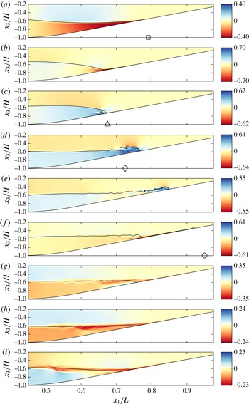
Snapshots in time of the laterally averaged cross-shore velocity structure for breaking wave case 3t1. The colour scale for each panel is based on the maximum absolute value of the cross-shore velocity at the given time step normalized by the linear wave speed,
 $\pm |u_{1}|_{max}/c_{0}$
. A contour line of the
 ${\it\rho}={\it\rho}_{0}$
isopycnal is shown for reference. Also shown are the cross-shore location of the breakpoint (c, ▵), the location of the formation of the upslope surge (d, ♢), the initial intersection of the pycnocline and the slope (a, ▫) and the maximum onshore location of the upslope surge (f, ○). These are referenced in figures 5, 6(b) and 15.

3. Cross-shore transport
3.1. Physical description
When internal gravity waves interact with sloping bathymetry, the induced velocity field acts to transport mass predominantly in the cross-shore (
 $x_{1}$
) direction. We therefore begin with a general description of cross-shore transport that is based on the results of case 3t1. The cross-shore velocity field
 $u_{1}$
, normalized by the linear wave speed
 $c_{0}$
, is shown over time for case 3t1 in figure 3. It should be noted that these results were originally presented in Arthur & Fringer (Reference Arthur and Fringer2014) (see their figure 2), but are included here for clarity. As the leading face of the wave reaches the slope, downslope velocities are concentrated in the lower layer (figure 3
a) and are eventually confined to the thin region between the interface and the bottom (figure 3
b), creating a strong downslope jet with
 $u_{max}/c_{0}=0.71$
. This jet interacts with the upslope velocities with
 $u_{max}/c_{0}=0.79$
underneath the rear shoulder of the wave to cause the overturning indicative of wave breaking (figure 3
c). After breaking, dense fluid continues to surge upslope as a bore or bolus with
 $u_{max}/c_{0}=0.65$
. Flow is also directed up and over the nose of the upslope surge, creating offshore flow in the upper layer (figure 3
d,e). Once the surge reaches its maximum upslope location, a second downslope jet forms as dense fluid relaxes back down the slope (figure 3
f), reaching
 $u_{max}/c_{0}=0.62$
. Due to mixing during the upslope surge, this downstream jet is less dense than the initial lower-layer fluid, causing it to detach from the slope (figure 3
g) and flow offshore along the pycnocline as an intrusion (figure 3
h,i) with
 $u_{max}/c_{0}=0.24$
. Also shown in figure 3 (as well as in figures 4, 12 and 13) are labels indicating the cross-shore location of the breakpoint (c, ▵), the location of the formation of the upslope surge (d, ♢), the initial intersection of the pycnocline and the slope (a, ▫) and the maximum onshore location of the upslope surge (f, ○). These locations are approximate and were chosen by visual inspection; they are displayed for reference in figures 5, 6(b) and 15.
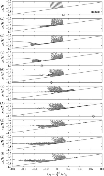
Currents induced by the breaking wave transport particles in both the onshore and offshore directions. Figure 4 shows the positions of the particles in the plume with initial locations shown in figure 1(c) over time for case 3t1. We note that this figure only shows the (
 $x_{1},x_{3}$
) positions, or a side view, of the particles, despite the fact that they propagate in the lateral (
 $x_{2}$
) direction due to three-dimensional turbulence. As the wave begins to interact with the slope, particles are transported offshore in the lower layer and slightly onshore in the upper layer (figure 4
a–c). After the wave breaks, the upslope surge of dense fluid transports particles onshore. Upper-layer fluid is directed up and over the nose of the upslope surge, carrying a thin layer of particles offshore along the pycnocline (figure 4
d,e). Once the surge reaches its maximum upslope location, the relaxation of dense fluid begins to carry particles back downslope (figure 4
f). When the jet detaches from the slope as an intrusion, particles are transported further offshore along the pycnocline (figure 4
f–i).
Snapshots in time of a plume of particles from breaking wave case 3t1. A side (
 $x_{1},x_{3}$
) view of the three-dimensional particle positions is shown. The cross-shore position
 $x_{1}$
is presented relative to the initial mean position of the plume
 $\overline{x}_{1}^{p,0}$
and normalized by the wave length scale
 $L_{w}$
. A contour line of the
 ${\it\rho}={\it\rho}_{0}$
isopycnal is shown for reference. The panel labelled ‘Initial’ shows the initial particle plume; panels (a–i) correspond to the same times as in figure 3. Also shown are the cross-shore location of the breakpoint (c, ▵), the location of the formation of the upslope surge (d, ♢), the initial intersection of the pycnocline and the slope (initial, ▫) and the maximum onshore location of the upslope surge (f, ○). These are referenced in figures 5, 6(b) and 15.

Over the course of the breaking event, onshore transport occurs along the bottom within the upslope surge of dense fluid. Offshore transport occurs along the pycnocline, initially due to flow over the nose of the upslope surge and ultimately due to the offshore intrusion of intermediate-density fluid. Above the pycnocline, the onshore transport is minimal and decreases towards the surface. The shape of the plume at the end of the breaking event resembles the plume in the numerical dye study of Nakayama & Imberger (Reference Nakayama and Imberger2010). Their study examined the cumulative effect of multiple periodic internal waves breaking on a slope, as opposed to the single wave of depression considered here.
While the particle plume discussed above provides a good visualization of cross-shore transport, analysis of the plume only allows for the quantification of transport of particles initialized near the breaking region. The particles initialized over the length of the slope (see figure 1
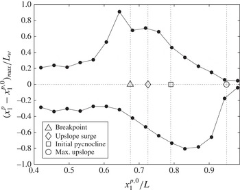
c) provide a more complete description of particle motion during the breaking event. In particular, these particles allow us to characterize the cross-shore variation in cross-shore transport, as shown in figure 5 for case 3t1. It should be noted that although particles move in three dimensions due to turbulence, figure 5 considers only the cross-shore component of this motion. These results were calculated by binning particles based on their initial cross-shore positions
 $x_{1}^{\,p,0}$
. Sixteen bins of length
 $L_{bin}/L=0.0375$
were used between
 $x_{1}/L=0.4$
and
 $x_{1}/L=1$
. Particles initialized just offshore of the breakpoint travel the furthest onshore (
 $0.90L_{w}$
), as they are carried from this point to the maximum onshore location of the upslope surge. The maximum onshore transport then decreases in the onshore direction, as the distance between the initialized particle and the maximum onshore location of the upslope surge decreases. The maximum offshore transport (
 $0.80L_{w}$
) is found for particles initialized near the intersection of the pycnocline and the slope. Offshore transport then decreases in both the onshore and offshore directions. The particles initialized in this region that travel the furthest offshore are mixed into intermediate-density fluid during breaking and are then carried offshore by the resulting intrusion.
Maximum onshore and offshore transport
 $(x_{1}^{\,p}-x_{1}^{\,p,0})_{max}$
, normalized by the wave length scale
 $L_{w}$
, as a function of the initial cross-shore position
 $x_{1}^{\,p,0}$
for breaking wave case 3t1. Onshore transport is positive, while offshore transport is negative. Also shown are the breakpoint, the location of the formation of the upslope surge, the initial intersection of the pycnocline and the slope, and the maximum onshore location of the upslope surge.

3.2. Effective cross-shore dispersion
The cross-shore transport of particles is quantified with an effective cross-shore dispersion coefficient, defined as
 $$\begin{eqnarray}D_{1}=\frac{1}{2}\frac{\partial ({\it\sigma}_{1}^{p})^{2}}{\partial t}-{\it\kappa},\end{eqnarray}$$
where
 $({\it\sigma}_{1}^{p})^{2}$
is the cross-shore variance of particles. Here, we calculate the time-averaged cross-shore dispersion over the course of the breaking event as
 $$\begin{eqnarray}\overline{D}_{1}=\frac{1}{2}\frac{({\it\sigma}_{1}^{p,f})^{2}-({\it\sigma}_{1}^{p,i})^{2}}{t_{f}-t_{i}}-{\it\kappa},\end{eqnarray}$$
where
 $t_{i}$
is defined as the time at which
 $({\it\sigma}_{1}^{p})^{2}>1.2({\it\sigma}_{1}^{p,0})^{2}$
(when
 $({\it\sigma}_{1}^{p})^{2}$
begins to increase above its initial value
 $({\it\sigma}_{1}^{p,0})^{2}$
) and
 $t_{f}$
is defined as the end of the breaking event.
Cross-shore variance results are binned as in § 3.1 such that
 $({\it\sigma}_{1}^{p})^{2}$
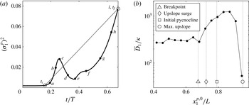
represents the cross-shore variance of the particles that were initialized in each bin. An example plot of
 $({\it\sigma}_{1}^{p})^{2}$
over time for case 3t1 is shown in figure 6(a) for the bin centred at
 $x_{1}/L=0.83$
(this corresponds to the bin with the maximum cross-shore dispersion, see figure 6
b). The curve in figure 6(a) is qualitatively similar for each bin, and shows non-monotonic behaviour of
 $({\it\sigma}_{1}^{p})^{2}$
with time due to the oscillatory nature of the breaking wave. The first increase in
 $({\it\sigma}_{1}^{p})^{2}$
occurs due to the initial rundown of the wave as it approaches the slope (figure 4
a–c). After breaking,
 $({\it\sigma}_{1}^{p})^{2}$
decreases as the upslope surge brings most of the particles back to roughly their initial positions (figure 4
d). Despite the decrease in
 $({\it\sigma}_{1}^{p})^{2}$
from point
 $c$
to point
 $d$
, a small net increase in
 $({\it\sigma}_{1}^{p})^{2}$
occurs from time
 $t_{i}$
to point
 $d$
. As the upslope surge carries particles further onshore in the lower layer and flow over the upslope surge carries particles offshore in the upper layer,
 $({\it\sigma}_{1}^{p})^{2}$
again increases (figure 4
e). Ultimately,
 $({\it\sigma}_{1}^{p})^{2}$
increases until the end of the breaking event due to transport by the offshore intrusion of mixed fluid (figure 4
f–i). Despite the oscillatory nature of
 $({\it\sigma}_{1}^{p})^{2}$
over time, the time-average cross-shore dispersion
 $\overline{D}_{1}$
defined in (3.2) captures the net increase in
 $({\it\sigma}_{1}^{p})^{2}$
due to the breaking event as a whole.
Effective cross-shore dispersion results for breaking wave case 3t1. (a) The cross-shore variance
 $({\it\sigma}_{1}^{p})^{2}$
as a function of time for the bin centred at
 $x_{1}/L=0.83$
. The locations of
 $t_{i}$
and
 $t_{f}$
used in the calculation of
 $\overline{D}_{1}$
are shown for reference (○). Labels (
 $a$
–
 $i$
) correspond to the time snapshots shown in figures 3 and 4. (b) The effective cross-shore dispersion
 $\overline{D}_{1}$
as a function of the initial cross-shore position
 $x_{1}^{\,p,0}$
. Also shown are the breakpoint, the location of the formation of the upslope surge, the initial intersection of the pycnocline and the slope, and the maximum onshore location of the upslope surge.

The cross-shore dispersion results
 $\overline{D}_{1}$
for case 3t1 are shown in figure 6(b) as a function of the initial cross-shore position. The strong onshore and offshore transport during the breaking event results in a net cross-shore dispersion of particles. As expected from figure 5, the largest
 $\overline{D}_{1}$
values occur in the breaking region, peaking at roughly 1500 times the molecular diffusivity
 ${\it\kappa}$
near the initial intersection of the pycnocline and the slope. From here,
 $\overline{D}_{1}$
values decrease in both the onshore and offshore directions. In the onshore direction,
 $\overline{D}_{1}$
values decrease rapidly beyond the maximum onshore position of the upslope surge. In the offshore direction outside of the breaking region,
 $\overline{D}_{1}$
values level out at roughly 300 times
 ${\it\kappa}$
.
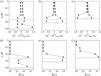
Maximum onshore and offshore transport (a–c) and effective cross-shore dispersion (d–f) as a function of depth for breaking wave case 3t1. Results are shown for three cross-shore bins centred at
 $x_{1}/L=0.64$
(a,d, the location of maximum onshore transport in figure 5),
 $x_{1}/L=0.76$
(b,e, an intermediate location with similar onshore and offshore transport values) and
 $x_{1}/L=0.83$
(c, f, the location of maximum offshore transport in figure 5). The maximum onshore and offshore transport is normalized by the wave length scale
 $L_{w}$
. Also shown are the local depth of the initial pycnocline (– – –) and the local bottom depth on the offshore side of the cross-shore bin (——).

3.3. Depth variation
The cross-shore transport of particles during wave breaking shows a clear variation with depth (see figure 4 and Nakayama & Imberger Reference Nakayama and Imberger2010). However, this depth variation is not considered in the maximum onshore and offshore transport and effective cross-shore dispersion results presented above, since these are representative of the maximum cross-shore transport and dispersion throughout the water column. We therefore recalculate these values for several representative cross-shore bins, now binning particles by their initial depth
 $x_{3}^{\,p,0}$
as well. We use vertical bins with a height of
 $h_{bin}/H=0.09$
; the number of vertical bins used depends on the local depth of the given cross-shore bin. The maximum onshore and offshore transport and effective cross-shore dispersion results are presented as a function of depth in figure 7. Results are shown for three cross-shore bins centred at
 $x_{1}/L=0.64$
(the location of maximum onshore transport in figure 5),
 $x_{1}/L=0.76$
(an intermediate location with similar onshore and offshore transport values) and
 $x_{1}/L=0.83$
(the location of maximum offshore transport in figure 5).
As expected, cross-shore transport and dispersion are low in the upper layer and near the surface (above roughly
 $x_{3}/H=-0.4$
), where the wave induces mostly uniform onshore and offshore velocities. Here, the maximum transport
 $(x_{1}^{p}-x_{1}^{p,0})_{max}\leqslant 0.1L_{w}$
and the effective dispersion
 $\overline{D}_{1}\approx {\it\kappa}$
. Transport and dispersion increase near the pycnocline and near the bottom, where strong onshore and offshore transport is induced by wave breaking. At the deepest location shown in figure 7(a,d) (
 $x_{1}/L=0.64$
), there is a separation between the transport near the pycnocline and the transport near the bottom. Near the pycnocline, particles move roughly
 $0.25L_{w}$
onshore during breaking and the beginning of the upslope surge (see figure 4
c,d), and roughly
 $0.30L_{w}$
during the offshore intrusion of mixed fluid at the end of the event (see figure 4
g–i). This results in an effective dispersion of roughly
 $400{\it\kappa}$
near the pycnocline. Near the bottom, the overall maximum onshore transport of roughly
 $0.90L_{w}$
occurs due to particles being carried onshore by the upslope surge. The maximum offshore transport near the bottom is similar to that near the pycnocline (roughly
 $0.30L_{w}$
), but it occurs during the initial rundown of dense fluid before breaking (see figure 4
a,b). The resulting dispersion near the bottom is roughly
 $300{\it\kappa}$
. Thus, although the maximum transport near the bottom is roughly three times that near the pycnocline, the net spreading of particles is approximately equal in both locations. In the middle of the lower layer (
 $x_{3}/H=-0.67$
), the net effect of the breaking event on transport is smaller. Maximum transport is reduced to roughly
 $0.05L_{w}$
onshore and
 $0.30L_{w}$
offshore, resulting in a reduced dispersion of roughly
 $20{\it\kappa}$
.
At the intermediate-depth location shown in figure 7(b,e) (
 $x_{1}/L=0.76$
), the initial pycnocline is close to the bottom. Maximum transport and dispersion values are therefore concentrated near the pycnocline and near the bottom where velocities are strongest during breaking. The maximum onshore transport due to the upslope surge is roughly
 $0.65L_{w}$
and the maximum offshore transport due to the offshore intrusion of mixed fluid is also roughly
 $0.65L_{w}$
. The resulting dispersion is roughly
 $800{\it\kappa}$
, slightly larger than the maximum seen at the deeper location. The shallowest location, shown in figure 7(c, f) (
 $x_{1}/L=0.83$
), is onshore of the initial intersection of the pycnocline and the slope. Transport and dispersion are thus elevated near the bottom, where the flow is affected by the upslope surge and its subsequent relaxation downslope. The maximum transport is dominated by offshore transport of roughly
 $0.80L_{w}$
, which is the overall maximum value during the event, since particles are entrained in the offshore flow of mixed fluid after breaking. Particles are transported only
 $0.35L_{w}$
onshore as the upslope surge passes by. The resulting dispersion (roughly
 $1600{\it\kappa}$
) is approximately twice as large as that seen at the intermediate-depth location (figure 7
e). This indicates that a relatively large number of particles initialized at this cross-shore location are transported offshore by the intrusion of mixed fluid, increasing the local binned variance
 $({\it\sigma}_{1}^{p})^{2}$
. It should be noted that while the overall maximum onshore and offshore transport values in figure 7(a–c) are equal to the maximum values shown in figure 5 at the corresponding cross-shore locations, the maximum effective dispersion values shown in figure 7(d–f) are generally larger than those shown in figure 6(b). This is because without vertical binning,
 $({\it\sigma}_{1}^{p})^{2}$
, and thus
 $\overline{D}_{1}$
, is reduced by particles near the surface that do not spread in the cross-shore direction.
3.4. Intermediate nepheloid layer formation
The layer of particles transported offshore along the pycnocline by the breaking wave in figure 4 resembles an INL. These features have been observed in the field (McPhee-Shaw et al.
Reference McPhee-Shaw, Sternberg, Mullenbach and Ogston2004; McPhee-Shaw Reference McPhee-Shaw2006; Cheriton et al.
Reference Cheriton, McPhee-Shaw, Shaw, Stanton, Bellingham and Storlazzi2014), as well as numerically (Bourgault et al.
Reference Bourgault, Kelley and Galbraith2005; Nakayama & Imberger Reference Nakayama and Imberger2010; Bourgault et al.
Reference Bourgault, Morsilli, Richards, Neumeier and Kelley2014) and in the laboratory (Ivey & Nokes Reference Ivey and Nokes1989; Helfrich Reference Helfrich1992; McPhee-Shaw & Kunze Reference McPhee-Shaw and Kunze2002; Nakayama & Imberger Reference Nakayama and Imberger2010). The use of particles initialized over the entire slope (figure 1
c) in our simulations allows the formation of INLs to be considered in terms of irreversible mixing driven by wave breaking. Specifically, we divide the domain into three regions based on the density
 ${\it\rho}$
. The intermediate region is defined as
 ${\it\rho}_{0}-f{\rm\Delta}{\it\rho}/2<{\it\rho}<{\it\rho}_{0}+f{\rm\Delta}{\it\rho}/2$
, while the top and bottom regions are defined as
 ${\it\rho}<{\it\rho}_{0}-f{\rm\Delta}{\it\rho}/2$
and
 ${\it\rho}>{\it\rho}_{0}+f{\rm\Delta}{\it\rho}/2$
respectively. The parameter
 $f$
is a fraction of the total density difference
 ${\rm\Delta}{\it\rho}$
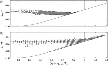
and is chosen to be 0.7. The INL is then defined to include particles within the intermediate region at the end of the breaking event. The INL is depicted in figure 8(a) for case 3t1.
Particles that make up the INL for breaking wave case 3t1: (a) the final positions of the particles within the INL at
 $t=t_{f}$
and (b) their initial positions at
 $t=t_{0}$
. Each plot shows contours of the intermediate region as well as a vertical line at the cross-shore position of the initial intersection of the pycnocline and the slope
 $x_{1,pyc}$
.

A benefit of defining the INL using particles in this way is the ability to examine INL composition based on particle initial positions, as shown in figure 8(b). In addition to the particles that are initialized within the intermediate-density region, the INL consists mostly of particles that begin in the breaking region and are mixed into the intermediate-density region during breaking and the upslope surge. This includes particles between the initial interface and the bottom that are swept downslope before getting caught in the upslope surge. It also includes particles above the initial interface that are entrained in the upslope surge as it propagates and are ultimately carried offshore by the relaxation of dense fluid downslope.
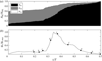
We examine the entrainment of particles into the intermediate region during breaking by keeping track of the fraction of INL particles in each region
 $N_{R}/N_{\mathit{INL}}$
over time, with
 $R=\mathit{int}$
,
 $top$
and
 $bot$
. This result is shown in figure 9(a) for case 3t1. Also shown in figure 9(b) is the volume-integrated effective irreversible mixing rate
 ${\it\phi}_{e}$
for case 3t1, as computed in Arthur & Fringer (Reference Arthur and Fringer2014). Initially, the majority of particles that end up in the INL are within the top and bottom regions, while a small fraction (approximately 8 %) are within the intermediate region. The fraction of particles in the intermediate region
 $N_{int}/N_{\mathit{INL}}$
then increases monotonically over the course of the breaking event as particles from the top and bottom regions are mixed into the intermediate region. Several processes lead to this entrainment. First, as the wave begins to overturn and break, a small spike in irreversible mixing is seen and particles from the bottom region are entrained into the intermediate region (figure 9
b, point
 $c$
). Then, as the upslope surge forms and propagates upslope, irreversible mixing increases rapidly and billows at the interface lead to increased entrainment from the top region into the intermediate region (figure 9
b, points
 $d$
–
 $f$
). Entrainment continues until
 $N_{int}/N_{\mathit{INL}}=1$
at the end of the breaking event. We note that irreversible mixing, and thus the entrainment of particles into the INL, is dependent on the Prandtl number
 $Pr={\it\nu}/{\it\kappa}$
, which is 7 for temperature and 700 for salt. However, we use
 $Pr=1$
here due to the increased computational effort associated with resolving mixing for smaller values of
 ${\it\kappa}$
.
The entrainment of particles into the intermediate-density region over time for breaking wave case 3t1: (a) a stacked area plot of the fraction of INL particles
 $N_{R}/N_{\mathit{INL}}$
within the intermediate (
 $R=\mathit{int}$
), top (
 $R=\mathit{top}$
) and bottom (
 $R=\mathit{bot}$
) regions over time and (b) the volume-integrated effective irreversible mixing rate
 ${\it\phi}_{e}$
as computed in Arthur & Fringer (Reference Arthur and Fringer2014). Labels (
 $a$
–
 $i$
) correspond to the time snapshots shown in figures 3 and 4.

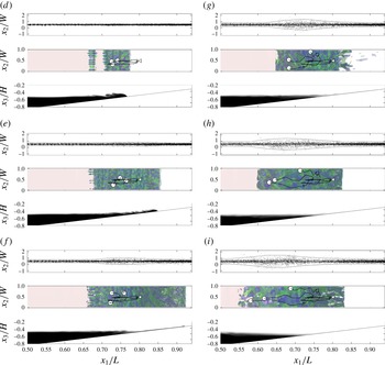
Lateral transport of particles, along with the density and vorticity structure, of breaking wave case 3t1. Each panel of the figure includes three parts. The first part shows a top view (
 $x_{1}{-}x_{2}$
) of all particles. Particles are shown to extend beyond the lateral boundaries of the domain
 $x_{2}/W=(0,1)$
due to lateral periodicity. Also included are contours of
 $x_{2}/W=0.5\pm 3{\it\sigma}_{2}^{p}/W$
, where
 ${\it\sigma}_{2}^{p}$
is calculated using the same bins as in figures 12 and 13, representing the lateral boundary of the particle plume. The second part shows a top view of the breaking wave that includes isosurfaces of
 ${\it\rho}={\it\rho}_{0}$
(red),
 ${\it\omega}_{1}/{\it\omega}_{0}=6$
(blue) and
 ${\it\omega}_{1}/{\it\omega}_{0}=-6$
(green). Also included are pathlines of three particles initialized at
 $x_{1}/L\approx 0.8$
and
 $x_{3}^{+}\approx 0.8$
(vertical grid points 8–10). The white dots represent the (
 $x_{1}{-}x_{2}$
) positions of the particles at the given time, while the white triangle represents their initial position. The third part shows a side view (
 $x_{1}{-}x_{3}$
) of the laterally averaged density structure. Here, (d–i) correspond to the time snapshots shown in figures 3 and 4.

4. Lateral transport
4.1. Three-dimensional particle dynamics
The lateral velocities induced by breaking allow for the lateral transport of particles. Figure 10 depicts this lateral transport over time for case 3t1, including a top view (
 $x_{1}{-}x_{2}$
) of the particles, a top view of the streamwise vorticity structure
 ${\it\omega}_{1}$
and a side view (
 $x_{1}{-}x_{3}$
) of the density structure. Before turbulence develops, lateral transport occurs only due to a random walk based on the molecular diffusivity
 ${\it\kappa}$
. Then, as the wave breaks, lateral variability develops regions of unstable stratification due to the lobe and cleft instability at the nose of the upslope surge and secondary convective instability within billows at the interface (Arthur & Fringer Reference Arthur and Fringer2014). Initially, this variability does not lead to enhanced lateral transport (figure 10
d). However, as the flow transitions to fully turbulent during the upslope surge (figure 10
e, f), lateral transport occurs at faster rate than that due to the molecular diffusivity. This lateral spreading continues as dense fluid from the upslope surge relaxes back downslope, causing a second burst of turbulence (figure 10
g). Turbulence then begins to dissipate, but the laterally spreading plume of particles continues to move offshore in the intrusion of mixed fluid (figure 10
f–i). It should be noted that in figure 10, particles are plotted outside of the lateral boundaries of the computational domain. This is because the lateral particle positions
 $x_{2}^{p}$
were adjusted to account for periodic boundary crossings by adding or subtracting the domain width
 $W$
.
The middle part of each panel of figure 10 also shows the pathlines of three particles initialized at
 $x_{1}/L\approx 0.8$
and
 $x_{3}^{+}\approx 0.8$
(vertical grid points 8–10). The white dots represent the (
 $x_{1}{-}x_{2}$
) positions of the particles at the given time. These particle paths highlight the effects of three-dimensionality on transport. First, the lateral motions of the particles are driven by the lateral velocities associated with the turbulent breakdown of the wave (this lateral transport is discussed further in §§ 4.2 and 4.3 below). Additionally, turbulence causes particles that are initialized at nearly the same location to end up in quite different cross-shore positions. Such variability in cross-shore transport is captured by the effective cross-shore dispersion
 $\overline{D}_{1}$
calculated in § 3.2. To confirm this, we observe that the cross-shore separation distance,
 ${\it\delta}x^{p}$
, of the three particles at the end of the simulation (as shown in figure 10
i) scales with the cross-shore dispersion length scale,
 $$\begin{eqnarray}{\it\delta}x^{p}/L\sim \sqrt{2\overline{D}_{1}t_{f}}/L\approx 0.1,\end{eqnarray}$$
where
 $\overline{D}_{1}\approx 10^{-3}~\text{m}^{2}~\text{s}^{-1}$
, as shown in figure 6(b) for
 $x_{1}/L\approx 0.8$
. We note that the random walk of particles also contributes to their separation; that is, if several particles were initialized at exactly the same position, the random walk would cause their trajectories to diverge.
4.2. Lateral turbulent diffusivity
The lateral spreading of particles during wave breaking can be characterized by a lateral turbulent diffusivity that is defined as
 $$\begin{eqnarray}D_{2T}=\frac{1}{2}\frac{\partial ({\it\sigma}_{2}^{p})^{2}}{\partial t}-{\it\kappa},\end{eqnarray}$$
where
 $({\it\sigma}_{2}^{p})^{2}$
is the lateral variance of particles. Here, we calculate the time-average lateral turbulent diffusivity for the breaking event as
 $$\begin{eqnarray}\overline{D}_{2T}=\frac{1}{2}\frac{({\it\sigma}_{2}^{p,f})^{2}-({\it\sigma}_{2}^{p,i})^{2}}{t_{f}-t_{i}}-{\it\kappa},\end{eqnarray}$$
where
 $t_{i}$
is defined as the first time at which
 $D_{2T}/{\it\kappa}-1\geqslant 0.05$
(i.e. when particles begin to spread at a rate above the molecular rate
 ${\it\kappa}$
) and
 $t_{f}$
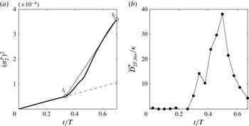
is defined as the end of the breaking event (see figure 11
a). A bulk value of
 $\overline{D}_{2T}$
calculated in this way using all particles initialized on the slope is approximately
 $4\times 10^{-6}~\text{m}^{2}~\text{s}^{-1}$
, or four times the molecular diffusivity
 ${\it\kappa}$
. However, because the turbulence that develops during wave breaking is not homogeneous, the bulk turbulent diffusivity is sensitive to the initial positions of the particles included in the calculation. In particular, particles in non-turbulent regions (e.g. most of the upper layer and the lower layer outside of the breaking region) spread only due to the molecular diffusivity, and therefore reduce the bulk turbulent diffusivity.
Examples of lateral variance and lateral turbulent diffusivity calculations for breaking wave case 3t1. (a) The bulk lateral variance
 $({\it\sigma}_{2}^{p})^{2}$
(calculated using all particles) as a function of time. The locations of
 $t_{i}$
and
 $t_{f}$
used in the calculation of
 $\overline{D}_{2T}$
are shown for reference (○), as is the molecular rate of increase of the lateral variance,
 $({\it\sigma}_{2}^{p})^{2}=2{\it\kappa}t$
(– – –). (b) Binned lateral turbulent diffusivity results
 $\overline{D}_{2T,bin}^{n}$
as a function of time for the bin centred at
 $x_{1}/L=0.75$
in figure 12.

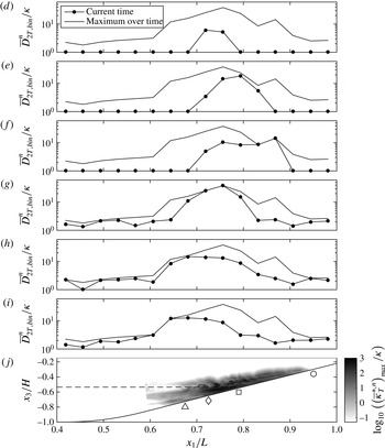
Binned lateral turbulent diffusivity calculations for breaking wave case 3t1. Panels (d–i) show
 $\overline{D}_{2T,bin}^{n}$
as a function of
 $x_{1}$
for the times corresponding to panels (d–i) in figures 3, 4 and 10, as well as the maximum
 $\overline{D}_{2T,bin}^{n}$
over the course of the breaking event
 $(\overline{D}_{2T,bin}^{n})_{max}$
. Panel (j) shows a side view (
 $x_{1}{-}x_{3}$
) of
 $\log _{10}((\overline{{\it\kappa}}_{T}^{\ast ,n})_{max}/{\it\kappa})$
, where ‘max’ indicates a maximum in time over the course of the breaking event, as a proxy for the strength of turbulence in the domain (see § 4.3). Also shown are the cross-shore location of the breakpoint (▵), the location of the formation of the upslope surge (♢), the initial intersection of the pycnocline and the slope (▫) and the maximum onshore location of the upslope surge (○) which are referenced in figures 5, 6(b) and 15, as well as the initial pycnocline (– – –).

A more representative turbulent diffusivity that accounts for the non-homogeneous nature of the turbulence during breaking can be calculated by binning particles in the cross-shore (
 $x_{1}$
) direction. We therefore create 16 cross-shore bins of length
 $L_{bin}/L=0.0375$
between
 $x_{1}/L=0.4$
and
 $x_{1}/L=1$
(as in § 3.1), in which we define binned values of the lateral variance of particles
 $({\it\sigma}_{2,bin}^{p,n})^{2}$
and the corresponding lateral turbulent diffusivity
 $\overline{D}_{2T,bin}^{n}$
. These values are a function of time because we reassign particles to bins after every
 ${\rm\Delta}n=1000$
time steps (
 $t/T=0.04$
). If particles are not re-binned, the number of particles in each bin can change over time due to cross-shore transport, potentially leading to non-monotonically increasing values of
 $({\it\sigma}_{2,bin}^{p,n})^{2}$
. Re-binning particles every
 $t/T=0.04$
ensures the monotonicity of
 $({\it\sigma}_{2,bin}^{p,n})^{2}$
because the amount of cross-shore transport that occurs over this time period is small. The binned lateral turbulent diffusivities are then calculated for each time period
 ${\rm\Delta}n$
as
 $$\begin{eqnarray}\overline{D}_{2T,bin}^{n}=\frac{1}{2}\frac{({\it\sigma}_{2,bin}^{p,n+{\rm\Delta}n})^{2}-({\it\sigma}_{2,bin}^{p,n})^{2}}{t^{n+{\rm\Delta}n}-t^{n}}-{\it\kappa},\end{eqnarray}$$
for
 $n=(0,{\rm\Delta}n,2{\rm\Delta}n,\ldots )$
. The choice of
 ${\rm\Delta}n$
does not significantly affect the
 $\overline{D}_{2T,bin}^{n}$
results as long as it is small enough to ensure monotonicity of
 $({\it\sigma}_{2,bin}^{p,n})^{2}$
over that time. An example of
 $\overline{D}_{2T,bin}^{n}$
as a function of time is shown in figure 11(b) for the bin centred at
 $x_{1}/L=0.75$
. It should be noted that
 $\overline{D}_{2T,bin}^{n}\geqslant 0$
because
 $({\it\sigma}_{2,bin}^{p,n})^{2}$
is monotonically increasing. It begins to increase above zero when the flow becomes turbulent within the bin at
 $t/T=0.25$
. It then increases as turbulence grows within the bin due to the upslope surge, decreasing slightly at
 $t/T=0.38$
as the upslope surge exits the upslope boundary of the bin. It reaches a peak of nearly 40 times the molecular value
 ${\it\kappa}$
at
 $t/T=0.50$
as the dense fluid from the upslope surge relaxes back downslope, and then decreases as turbulence decays.
Binned lateral turbulent diffusivity results
 $\overline{D}_{2T,bin}^{n}$
as a function of cross-shore position are shown over time in figure 12. Over the course of the breaking event, the lateral turbulent diffusivity is elevated within the breaking region, which extends from roughly
 $x_{1}/L=0.6$
to
 $x_{1}/L=0.95$
. This overlaps with the most turbulent region of the domain, marked by darker colours in figure 12(j) (see § 4.3 for further discussion of the value used as a proxy for turbulence). However, the location of elevated turbulent diffusivity changes with time due to the non-homogeneous nature of turbulence during wave breaking. The binned lateral turbulent diffusivity
 $\overline{D}_{2T,bin}^{n}$
is first elevated near and onshore of the breakpoint (figure 12
d). As the upslope surge forms and travels upslope, the elevated region of
 $\overline{D}_{2T,bin}^{n}$
moves onshore (figure 12
e). Then, as the fluid from the upslope surge relaxes back downslope,
 $\overline{D}_{2T,bin}^{n}$
increases and reaches a maximum of roughly 40 times the molecular diffusivity
 ${\it\kappa}$
at
 $x_{1}/L=0.75$
(figure 12
f,g). As mixed fluid continues to flow offshore in the intrusion, the region of elevated
 $\overline{D}_{2T,bin}^{n}$
extends further offshore (figure 12
h,i).
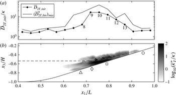
Lateral turbulent diffusivity calculations as a function of initial particle position for breaking wave case 3t1. Panel (a) shows
 $\overline{D}_{2T,init}$
as a function of cross-shore position
 $x_{1}$
. The values labelled 8–13 correspond to points in figure 14(b). The maximum of
 $\overline{D}_{2T,bin}^{n}$
over the course of the breaking event
 $(\overline{D}_{2T,bin}^{n})_{max}$
(as in figure 12) is also shown for comparison. Panel (b) shows a side view (
 $x_{1}{-}x_{3}$
) of
 $\text{log}_{10}(\overline{{\it\kappa}}_{T}^{\ast }/{\it\kappa})$
as a proxy for the strength of turbulence in the domain (see § 4.3). Also shown are the cross-shore location of the breakpoint (▵), the location of the formation of the upslope surge (♢), the initial intersection of the pycnocline and the slope (▫) and the maximum onshore location of the upslope surge (○) which are referenced in figures 5, 6(b) and 15, as well as the initial pycnocline (– – –).

While
 $\overline{D}_{2T,bin}^{n}$
provides a local measure of lateral turbulent spreading within each bin, a measure of particle spreading based on the initial positions of particles is also desirable. In particular, in the coastal ocean, it is useful to know how a biologically important scalar plume (e.g. nutrients, larvae, sediment or dissolved oxygen) at a given location may spread over the course of a wave breaking event. For this reason we define a lateral turbulent diffusivity
 $\overline{D}_{2T,init}$
that is calculated as in (4.3), but using particles binned by their initial cross-shore position
 $x_{1}^{\,p,0}$
. It should be noted that
 $t_{i}$
in (4.3) is now a bin-specific value (
 $t_{f}$
is the same for all bins). Thus,
 $\overline{D}_{2T,init}$
is a measure of lateral turbulent spreading as a function of initial cross-shore location. The
 $\overline{D}_{2T,init}$
results for breaking wave case 3t1 are shown in figure 13. It can be seen that
 $\overline{D}_{2T,init}$
reaches a maximum value of roughly 20 times the molecular diffusivity between
 $x_{1}/L=0.725$
and
 $x_{1}/L=0.75$
, near the formation of the upslope surge, and is elevated throughout the region covered by the upslope surge, where turbulence is most energetic (darker colours in figure 13
b, see § 4.3 for further discussion of the value used as a proxy for turbulence). Particles initialized in this region first spread laterally due to turbulence during the upslope surge (figure 10
e, f). They then experience more lateral spreading due to turbulence associated with intrusion of mixed fluid offshore (figure 10
g–i). Thus, as these particles are transported in the cross-shore direction, they experience the maximum possible combination of the local spreading rates
 $\overline{D}_{2T,bin}^{n}$
shown in figure 12. This is evidenced by the comparison of
 $\overline{D}_{2T,init}$
with the maximum of
 $\overline{D}_{2T,bin}^{n}$
over the course of the breaking event
 $(\overline{D}_{2T,bin}^{n})_{max}$
in figure 13(a). Particles initialized outside of the turbulent region do not experience as much or any local spreading as they move in the cross-shore direction, leading to lower values of
 $\overline{D}_{2T,init}$
.
4.3. Application of a generic length scale turbulence closure model
Many models exist to parameterize turbulence in situations when DNS is not feasible. Warner et al. (Reference Warner, Sherwood, Arango and Signell2005) presented a generic length scale method that combines several such models, where a turbulent eddy viscosity
 ${\it\nu}_{T}$
is estimated as
 $$\begin{eqnarray}{\it\nu}_{T}=c(2k)^{1/2}lS_{M}+{\it\nu}.\end{eqnarray}$$
Thus, the eddy viscosity scales as
 ${\it\nu}_{T}\sim k^{1/2}l$
, where
 $k$
is the turbulent kinetic energy and
 $l$
is a turbulent length scale. The
 ${\it\nu}_{T}$
calculation includes a stability function
 $S_{M}$
that accounts for the effects of shear and stratification, as well as a model coefficient
 $c$
that depends on the chosen stability function. Using DNS results for case 3t1, we evaluate the effectiveness of this model for capturing lateral spreading during the breaking event. We use a framework that is similar to that of Warner et al. (Reference Warner, Sherwood, Arango and Signell2005) and estimate
 ${\it\kappa}_{T}$
by directly calculating
 $k$
and
 $l$
. It should be noted that we set
 ${\it\kappa}_{T}={\it\nu}_{T}$
since the particles in our simulations are passive. We then compare
 ${\it\kappa}_{T}$
with the lateral turbulent diffusivity values calculated using particle tracking in § 4.1. Thus, we estimate the turbulent diffusivity with
 $$\begin{eqnarray}{\it\kappa}_{T}=C(2k)^{1/2}l=C{\it\kappa}_{T}^{\ast },\end{eqnarray}$$
where
 $C$
is a constant,
 $l$
is a turbulent length scale and
 ${\it\kappa}_{T}^{\ast }=(2k)^{1/2}l$
. In order to account for the effects of stratification and the presence of the bottom boundary on the turbulent length scale, we choose
 $l=\text{min}(L_{T},L_{O},L_{b})$
, where
 $L_{T}=k^{3/2}/{\it\epsilon}$
is the scale of the energetic eddies,
 $L_{O}=({\it\epsilon}/N^{3})^{1/2}$
is the Ozmidov scale and
 $L_{b}$
is the local vertical distance to the bottom wall. As in Arthur & Fringer (Reference Arthur and Fringer2014), turbulent quantities are defined as a departure from the lateral average, such that the velocity
 $u_{i}=\langle u_{i}\rangle +u_{i}^{\prime }$
, where
 $\langle u_{i}\rangle$
is the laterally averaged velocity and
 $u_{i}^{\prime }$
is the fluctuation about the lateral average. The turbulent quantities
 $k$
and
 ${\it\epsilon}$
are then calculated as
 $$\begin{eqnarray}\displaystyle & k={\textstyle \frac{1}{2}}\langle u_{i}^{\prime }u_{i}^{\prime }\rangle , & \displaystyle\end{eqnarray}$$
 $$\begin{eqnarray}\displaystyle & {\it\epsilon}=2{\it\nu}\langle s_{ij}^{\prime }s_{ij}^{\prime }\rangle , & \displaystyle\end{eqnarray}$$
 $s_{ij}^{\prime }=((\partial u_{i}^{\prime }/\partial x_{j})+(\partial u_{j}^{\prime }/\partial x_{i}))/2$
.
To facilitate comparison of
 ${\it\kappa}_{T}^{\ast }$
, which is defined for all
 $x_{1}$
,
 $x_{3}$
and
 $t$
, with
 $\overline{D}_{2T,bin}^{n}$
, which is defined for each cross-shore bin and time interval
 ${\rm\Delta}n$
, we define
 $$\begin{eqnarray}(\overline{{\it\kappa}}_{T}^{\ast ,n})_{bin}=\max _{bin}\left(\frac{1}{t^{n+{\rm\Delta}n}-t^{n}}\int _{t^{n}}^{t_{n+{\rm\Delta}n}}{\it\kappa}_{T}^{\ast }\,\text{d}t\right),\end{eqnarray}$$
for
 $n=(0,{\rm\Delta}n,2{\rm\Delta}n,\ldots )$
. Thus,
 $\overline{{\it\kappa}}_{T}^{\ast ,n}$
is the time average of
 ${\it\kappa}_{T}^{\ast }$
over each time interval
 ${\rm\Delta}n$
and
 $(\overline{{\it\kappa}}_{T}^{\ast ,n})_{bin}$
is the maximum of
 $\overline{{\it\kappa}}_{T}^{\ast ,n}$
in each cross-shore bin. Similarly, to facilitate comparison of
 ${\it\kappa}_{T}^{\ast }$
with
 $\overline{D}_{2T,init}$
, which is defined for each cross-shore bin as an average over
 $t_{i}$
to
 $t_{f}$
, we define
 $$\begin{eqnarray}(\overline{{\it\kappa}}_{T}^{\ast })_{init}=\max _{bin}\left(\frac{1}{t_{f}-t_{i}}\int _{t_{i}}^{t_{f}}{\it\kappa}_{T}^{\ast }\,\text{d}t\right).\end{eqnarray}$$
Thus,
 $\overline{{\it\kappa}}_{T}^{\ast }$
is the time average of
 ${\it\kappa}_{T}^{\ast }$
between
 $t_{i}$
and
 $t_{f}$
, and
 $(\overline{{\it\kappa}}_{T}^{\ast })_{init}$
is the maximum of
 $\overline{{\it\kappa}}_{T}^{\ast }$
in each cross-shore bin.
Comparisons of
 $\overline{D}_{2T,bin}^{n}$
with
 $(\overline{{\it\kappa}}_{T}^{\ast ,n})_{bin}$
and
 $\overline{D}_{2T,init}$
with
 $(\overline{{\it\kappa}}_{T}^{\ast })_{init}$
are shown in figure 14 along with best-fit lines and the corresponding estimates of
 $C$
. Results for the local binned diffusivity
 $\overline{D}_{2T,bin}^{n}$
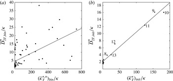
are relatively scattered (
 $R_{bin}^{2}=0.33$
), but tend to increase with
 $(\overline{{\it\kappa}}_{T}^{\ast ,n})_{bin}$
, with an estimated
 $C_{bin}$
value of 0.02. Results for the binned diffusivity based on initial particle position
 $\overline{D}_{2T,init}$
show remarkably good agreement with
 $(\overline{{\it\kappa}}_{T}^{\ast })_{init}$
(
 $R_{init}^{2}=0.98$
), with an estimated
 $C_{init}$
value of 0.08. It should be noted that the six points located along the best-fit line above
 $\overline{{\it\kappa}}_{t}^{\ast }/{\it\kappa}\approx 10$
labelled 8–13 in figure 14(b) correspond to bins with elevated values of
 $\overline{D}_{2T,init}$
in figure 13(a). These bins make up the most turbulent region of the domain, as shown in figure 13(b) (darker shades between
 $x_{1}/L=0.7$
and
 $x_{1}/L=0.9$
). Both estimated
 $C$
values are near the
 $c\approx 0.18$
value used with the stability functions of Canuto et al. (Reference Canuto, Howard, Cheng and Dubovikov2001) (see Warner et al.
Reference Warner, Sherwood, Arango and Signell2005) and the canonical value of
 $c=C_{{\it\mu}}/\sqrt{2}=0.09/\sqrt{2}\approx 0.06$
for
 $k{-}{\it\epsilon}$
models (Pope Reference Pope2000). This suggests good agreement between lateral turbulent diffusivity values estimated using particles and those estimated with a generic length scale turbulence model.
Comparison of lateral turbulent diffusivity calculations with estimates of
 ${\it\kappa}_{T}$
using a generic length scale turbulence closure model: (a)
 $\overline{D}_{2T,bin}^{n}$
versus
 $(\overline{{\it\kappa}}_{T}^{\ast ,n})_{bin}$
,
 $C_{bin}=0.02$
,
 $R_{bin}^{2}=0.33$
; (b)
 $\overline{D}_{2T,init}$
versus
 $(\overline{{\it\kappa}}_{T}^{\ast })_{init}$
,
 $C_{init}=0.08$
,
 $R_{init}^{2}=0.98$
. In each plot, the best-fit line used to calculate
 $C$
with the corresponding
 $R^{2}$
value is shown. Labels 8–13 in (b) correspond to bins with elevated values of
 $\overline{D}_{2T,init}$
in figure 13(a).

5. Two-dimensional model applications
5.1. Comparison of two- and three-dimensional k results
Thus far, we have discussed transport using a three-dimensional DNS (case 3t1). However, the computational expense associated with DNS makes the extension of our results to a larger parameter space impractical. It would, instead, be practical to make use of two-dimensional simulations for this purpose. For example, while case 3t1 took 145 h to run on 432 processors (63 000 CPU hours), the two-dimensional version (case 3) took just 16 h on 144 processors (2000 CPU hours). This is roughly a 96 % reduction in computational effort. Although two-dimensional simulations of breaking internal waves on slopes contain the unrealistic inverse energy cascade associated with two-dimensional turbulence, they are nonetheless qualitatively similar to three-dimensional simulations at this scale (Arthur & Fringer Reference Arthur and Fringer2014, see figure 13 therein). We therefore expect the cross-shore transport results from two- and three-dimensional simulations to be similar as well. By comparing the results of the two- and three-dimensional versions of case 3, we can determine whether it is reasonable to extend our results using two-dimensional simulations.
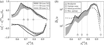
Cross-shore transport comparison between two- and three-dimensional simulations: (a) the maximum onshore and offshore transport, and (b) the effective cross-shore dispersion, both as functions of initial cross-shore position. For case 3t2, each cross-shore (
 $x_{1},x_{3}$
) slice of particles is considered separately; grey shading represents the range of values among all slices. For case 3, particle results are restricted to include only those particles that are initialized at the same (
 $x_{1},x_{3}$
) grid points as in case 3t2. Results for case 3t1, as in figures 5 and 6(b), are shown for reference. Also shown in each plot are the breakpoint, the location of the formation of the upslope surge, the initial intersection of the pycnocline and the slope, and the maximum onshore location of the upslope surge.

Figure 15 shows a comparison of cross-shore transport results between case 3t2 (three-dimensional) and case 3 (two-dimensional), including the maximum onshore and offshore transport as well as the effective cross-shore dispersion, both as functions of initial cross-shore position. It should be recalled from § 2.3 that case 3t2 includes particles initialized at the bottom 20 grid points in 10 cross-shore (
 $x_{1},x_{3}$
) slices over the width of the domain. We choose this initialization instead of that in case 3t1 (in which all particles are initialized along the lateral centreline) in order to better capture transport over the lateral extent of the flow. We note that because most of the cross-shore transport occurs near the bottom in the breaking region (figure 7), the maximum transport results in cases 3t1 and 3t2 are similar, as indicated by the dashed line in figure 15(a). The effective cross-shore dispersion for case 3t1, as shown by the dashed line in figure 15(b), is also similar to that in case 3t2. However, some differences arise because the cross-shore dispersion in case 3t1 is affected by particles in the upper layer. We consider each of the initial 10 cross-shore particle slices in case 3t2 separately. That is, we calculate maximum onshore and offshore transport, as well as the effective cross-shore dispersion, separately for each slice. Figure 15, therefore, shows the range of transport values among these 10 slices. Finally, in order to fairly compare case 3t2 with case 3, which has particles initialized at every vertical grid point over the entire length of the slope, we restrict the case 3 particle results to include only those particles that are initialized at the same (
 $x_{1},x_{3}$
) grid points as in case 3t2.
While the shapes of the maximum transport and effective dispersion curves for the two-dimensional (case 3) and three-dimensional (case 3t2) simulations are similar, some differences can be noted. In both simulations, the maximum onshore transport occurs for particles initialized just offshore of the breakpoint (figure 15 a). However, this maximum transport is slightly smaller for the three-dimensional simulation. The maximum offshore transport occurs, in both simulations, for particles initialized just onshore of the intersection of the pycnocline and the slope (figure 15 a). The maximum offshore transport is again slightly smaller for the three-dimensional simulation. The two-dimensional result essentially represents an upper bound for the cross-shore transport and dispersion, with the three-dimensional dispersion result being up to a factor of two smaller in the breaking region.
The differences in transport and dispersion are due to increased dissipation in the three-dimensional simulation. Arthur & Fringer (Reference Arthur and Fringer2014) found a 20 % increase in dissipation for their case 3 (identical to cases 3t1 and 3t2 here) due to turbulence during wave breaking. Roughly 60 % of this difference in dissipation occurs before
 $t/T=0.4$
, which is when the upslope surge reaches its maximum upslope position. The remaining 40 % occurs during the relaxation of mixed fluid downslope after the upslope surge and its subsequent intrusion offshore (figure 3
f–i, also see figure 15 after
 $t/T=0.4$
in Arthur & Fringer Reference Arthur and Fringer2014). Despite the differences between the two- and three-dimensional simulations, their qualitative agreement justifies the use of two-dimensional simulations to extend the cross-shore transport results of § 3 to a parameter space consisting of several wave amplitudes and bathymetric slopes, as described in the next section.
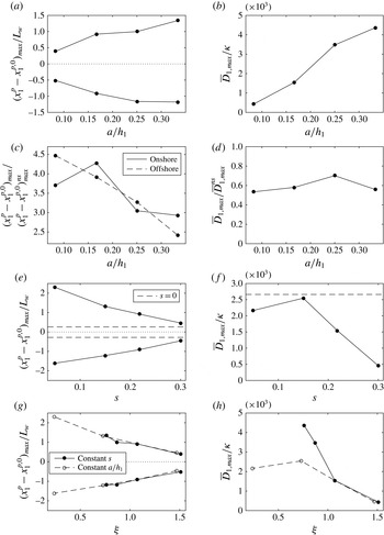
5.2. Variation of cross-shore transport with wave amplitude and bathymetric slope
The density and velocity structure associated with breaking internal waves is known to change with the amplitude of the incoming wave
 $a$
and the bathymetric slope
 $s$
(Boegman et al.
Reference Boegman, Ivey and Imberger2005; Arthur & Fringer Reference Arthur and Fringer2014). It follows that the magnitude of cross-shore transport induced by breaking waves should also change with these parameters. We investigate the changes in cross-shore transport as a function of
 $a$
and
 $s$
for two-dimensional cases 1–7 (summarized in table 1) using particles initialized over the length of the slope (see figure 1
c). We also consider how transport varies with the combined effect of
 $a$
and
 $s$
using the internal Iribarren number
 ${\it\xi}=s/\sqrt{a/L_{w}}$
, which has been used in the past to classify wave breakers (Boegman et al.
Reference Boegman, Ivey and Imberger2005; Aghsaee et al.
Reference Aghsaee, Boegman and Lamb2010), wave reflection (Bourgault & Kelley Reference Bourgault and Kelley2007; Aghsaee et al.
Reference Aghsaee, Boegman and Lamb2010) and turbulent mixing (Boegman et al.
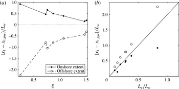
Reference Boegman, Ivey and Imberger2005; Arthur & Fringer Reference Arthur and Fringer2014). The results are summarized in figure 16. Onshore and offshore transport are quantified as the change in cross-shore particle position over the course of the breaking event
 $x_{1}^{\,p}-x_{1}^{\,p,0}$
. The effective cross-shore dispersion
 $\overline{D}_{1}$
is calculated with (3.2) using bins of the same length (and thus the same number of particles) as in § 3.1 for all cases.
Variation in cross-shore transport and dispersion for breaking wave cases 1–7. It should be noted that onshore transport is positive while offshore transport is negative. (a) Maximum onshore and offshore transport and (b) maximum effective cross-shore dispersion as functions of the incoming wave amplitude
 $a/h_{1}$
. (c) Maximum onshore and offshore transport and (d) maximum effective cross-shore dispersion, both relative to the corresponding no-slope (ns) case and as functions of
 $a/h_{1}$
. (e) Maximum onshore and offshore transport and (f) maximum effective cross-shore dispersion as functions of the bathymetric slope
 $s$
. The
 $s=0$
case with the same amplitude, case 3ns, is shown for reference. (g) Maximum onshore and offshore transport and (h) maximum effective cross-shore dispersion as functions of the internal Iribarren number
 ${\it\xi}$
.

First, we examine the variation in cross-shore transport with the non-dimensional incoming wave amplitude
 $a/h_{1}$
(keeping the slope
 $s$
constant) using the results of cases 1, 3, 4 and 5. The maximum onshore and offshore transport of particles increases with increasing
 $a/h_{1}$
(figure 16
a) due to the increased energy of the wave; as
 $a/h_{1}$
increases, the wave has more incoming energy to propagate onshore and more reflected energy to propagate back offshore. A similar result was presented by Bourgault et al. (Reference Bourgault, Morsilli, Richards, Neumeier and Kelley2014), who found a linear increase in the extent of offshore transport with increasing incoming wave energy. An increase in the effective cross-shore dispersion is also seen with increasing
 $a/h_{1}$
(figure 16
b).
In the absence of a slope, non-breaking internal solitary waves transport particles, and this transport also increases with
 $a/h_{1}$
(Lamb Reference Lamb1997; Gil & Fringer Reference Gil and Fringer2015). Therefore, it is useful to compare the cross-shore transport due to a breaking internal wave on a slope with that of the same wave propagating over a flat bottom. Although weakly nonlinear theory (e.g. KdV or eKdV) can be used to estimate transport by a wave over a flat bottom, fully nonlinear methods must be used for finite-amplitude internal solitary waves since they broaden with increased nonlinearity, an effect that significantly impacts the transport (Lamb Reference Lamb1997; Gil & Fringer Reference Gil and Fringer2015). We use the no-slope cases 1ns, 3ns, 4ns and 5ns to quantify transport due to the internal gravity waves in cases 1, 3, 4 and 5 in the absence of a slope. Figure 16(c,d) shows the maximum onshore and offshore transport, as well as the effective cross-shore dispersion, for cases 1, 3, 4 and 5 relative to the corresponding no-slope cases. The maximum cross-shore transport (figure 16
c) is larger in the sloping cases due to wave breaking. Both onshore and offshore transport are roughly four times larger in the sloping case for small to intermediate values of
 $a/h_{1}$
, with the ratio decreasing as
 $a/h_{1}$
increases. The relative onshore transport reaches a maximum at
 $a/h_{1}=0.17$
. This peak in the onshore transport is probably due to a peak in onshore energy flux, as described by Venayagamoorthy & Fringer (Reference Venayagamoorthy and Fringer2006): for smaller waves, there is little energy to transmit onshore, while for larger waves, dissipation and mixing increase, leading to a reduction in onshore energy transmission (see figure 10, Venayagamoorthy & Fringer Reference Venayagamoorthy and Fringer2006). In contrast to the onshore transport, the relative offshore transport decreases monotonically with increasing
 $a/h_{1}$
.
Interestingly, the maximum effective cross-shore dispersion (figure 16 d) is smaller in the sloping cases than in the no-slope cases. Because the breaking wave is a superposition of incident and reflected waves, a particle can be transported a large distance onshore by the incident wave before being transported back offshore by the reflected wave. The effect of the slope is therefore to reduce the effective cross-shore dispersion despite an increase in maximum onshore and offshore transport. In the limit of a vertical wall (infinite slope), there would be little energy loss during reflection, and the incident and reflected waves would be of similar amplitudes. As a result, the reflected wave would return a particle transported onshore by the incident wave back to roughly its initial location, leading to negligible effective cross-shore dispersion.
Next, we examine the variation in cross-shore transport with bathymetric slope
 $s$
(keeping
 $a/h_{1}$
constant) using the results of cases 2, 3, 6 and 7. Maximum onshore and offshore transport decrease with increasing
 $s$
(figure 16
e). Intuitively, onshore transport decreases with increasing
 $s$
because, for a steeper slope, the wave can travel a shorter onshore distance with the same amount of work against gravity. We might expect offshore transport to increase with increasing slope since more energy is reflected off of a steeper slope (see figure 20, Aghsaee et al.
Reference Aghsaee, Boegman and Lamb2010). However, if we define the end of the breaking event as the time at which dissipation reaches a minimum before the next breaking event begins (Arthur & Fringer Reference Arthur and Fringer2014), then this time scale increases with decreasing
 $s$
. Thus, more time is allowed for reflected wave energy to transport particles offshore on gentler slopes. This more than compensates for the decrease in reflected energy, causing offshore transport to increase with decreasing slope.
The maximum effective cross-shore dispersion (figure 16
f) peaks at roughly 2500 times
 ${\it\kappa}$
for the intermediate slope
 $s=0.15$
. For larger slopes, the effective dispersion decreases because there is less cross-shore transport. For smaller slopes, the effective dispersion decreases due to the behaviour of fission breakers (see table 1 and Arthur & Fringer Reference Arthur and Fringer2014). In this breaking regime, boluses transport a relatively small fraction of particles onshore by a large amount. However, the overall spreading of particles on the slope is comparatively small because the majority of particles are not affected by the boluses. The results for case 3ns, which has the same incoming wave amplitude as cases 2, 3, 6 and 7 but zero slope, are also included in figure 16(e, f) for reference. As discussed above in reference to figure 16(c,d), the presence of the slope increases the maximum cross-shore transport associated with the wave, but decreases the effective cross-shore dispersion.
Finally, we present the variation in cross-shore transport with the combined effect of incoming wave amplitude and bathymetric slope using the internal Iribarren number
 ${\it\xi}$
for cases 1–7. The maximum onshore and offshore transport values decrease with increasing
 ${\it\xi}$
(figure 16
g), as expected from figure 16(a,e), but are of the order of the wave length scale
 $L_{w}$
for all cases. Onshore transport values range from roughly
 $0.4L_{w}$
to
 $2.3L_{w}$
and offshore transport values range from roughly
 $0.4L_{w}$
to
 $1.6L_{w}$
. The effective cross-shore dispersion (figure 16
h) peaks at roughly 4500 times
 ${\it\kappa}$
for intermediate internal Iribarren numbers
 ${\it\xi}\approx 0.8$
, decreasing for larger values of
 ${\it\xi}$
due to either steeper slopes or smaller waves, and decreasing for smaller values of
 ${\it\xi}$
due to the occurrence of fission breakers.
The constant slope cases (1, 3, 4 and 5) and the constant amplitude cases (2, 3, 6 and 7), are presented separately in figure 16(g,h). While the maximum cross-shore transport shows a similar relationship to the internal Iribarren number
 ${\it\xi}$
regardless of whether
 $a/h_{1}$
or
 $s$
is held constant, the same is not true for the effective cross-shore dispersion. The sharp peak in effective cross-shore dispersion at
 ${\it\xi}\approx 0.8$
is associated with the occurrence of plunging breakers (cases 4 and 5, see table 1), which introduce more available potential energy to the flow than collapsing breakers with similar internal Iribarren numbers (cases 3 and 6). This discrepancy highlights a limitation of the internal Iribarren number, specifically that it may not uniquely define the properties of a breaking wave for a given wave amplitude and bathymetric slope. As noted in Arthur & Fringer (Reference Arthur and Fringer2014), properties such as the mixing efficiency or cross-shore transport of breaking internal waves on slopes might be more appropriately classified as a function of both the wave slope and the bathymetric slope, as in Aghsaee et al.’s (Reference Aghsaee, Boegman and Lamb2010) figure 6 for internal wave breaker types.
Despite its limitations, the internal Iribarren number provides a convenient way to compare idealized laboratory-scale transport results with those of a field-scale study. Bourgault et al. (Reference Bourgault, Kelley and Galbraith2005) used a two-dimensional model to study an internal solitary wave shoaling in the St Lawrence Estuary. With an initial wave amplitude of
 $a=15~\text{m}$
, an initial wave length scale of
 $L_{w}\approx 200~\text{m}$
and a bathymetric slope of
 $s=0.03{-}0.06$
(
 $1.9^{\circ }{-}3.3^{\circ }$
), their case had an internal Iribarren number of approximately 0.1–0.2. Although this resulted in a fission breaker that is qualitatively similar to the breaking wave in our case 7, there are several differences between the field-scale model of Bourgault et al. (Reference Bourgault, Kelley and Galbraith2005) and our laboratory-scale simulations. In terms of the initial density field, the field-scale case has a relatively thick interface, as well as a relatively deep lower layer. Additionally, Bourgault et al. (Reference Bourgault, Kelley and Galbraith2005) employed a quadratic drag law to parameterize the bottom friction, while we employ a no-slip bottom boundary condition with high near-bottom resolution. Field-scale models typically employ a quadratic drag law to account for the unresolved bottom boundary layer dynamics, for both hydrodynamically smooth and rough boundaries. Our simulations employ a no-slip condition because the boundary layer is resolved in both the two- and three-dimensional simulations. However, as noted in § 5.1, the two-dimensional simulations slightly overpredict the transport due to a lack of resolved three-dimensional dissipation during wave breaking. This effect could be accounted for with a turbulence model that parameterizes the unresolved dissipation along with a quadratic drag law that can effectively be tuned to produce a better match between the two- and three-dimensional results. Ultimately, Bourgault et al. (Reference Bourgault, Kelley and Galbraith2005) used a passive scalar to observe both onshore and offshore transport due to wave breaking. They observed a maximum onshore transport greater than
 $L_{w}$
within upslope-propagating boluses, and a maximum offshore transport of roughly
 $1.5L_{w}$
within an intermediate-density intrusion. These maximum cross-shore transport values agree quite well with what would be predicted by our two-dimensional simulations. Further comparisons with field-scale cases with low internal Iribarren numbers would require runs with lower slopes, which are more computationally expensive due to the need for a longer domain for a given depth.
5.3. Intermediate nepheloid layer composition
Despite the lack of three-dimensional turbulence in the two-dimensional simulations, particles are entrained into the pycnocline through diffusive processes that mimic three-dimensional turbulent entrainment. Therefore, the two-dimensional simulations can be used to qualitatively understand the impact of the internal Iribarren number on INL composition. Specifically, we would expect a change in the initial cross-shore extent of particles that are ultimately entrained into the INL as a function of the internal Iribarren number
 ${\it\xi}$
for the two-dimensional breaking wave cases 1–7. This change is relevant to biologically important scalars in the coastal ocean, as it could determine whether or not they are carried of the order of 1–10 km offshore (McPhee-Shaw Reference McPhee-Shaw2006) during an internal wave breaking event. Figure 17(a) shows the initial onshore and offshore extents of near-bottom particles that are entrained into the INL as a function of the internal Iribarren number
 ${\it\xi}$
. By visual inspection, we restrict this result to particles initialized near the bottom in order to remove the effect of particles initialized offshore near the pycnocline. As an example, figure 8(b) indicates a maximum onshore extent of roughly
 $0.3L_{w}$
and a maximum offshore extent of roughly
 $0.6L_{w}$
of near-bottom particles that are entrained into the INL; the particles extending offshore along the pycnocline in figure 8(b) are not considered. It should be recalled that the results in figure 8(b) are for case 3t1, and are similar to the results for case 3 shown in figure 17 (
 ${\it\xi}=1.07$
). Both the onshore and offshore extents of INL particles decrease with increasing
 ${\it\xi}$
due to either increasing
 $s$
or decreasing
 $a/h_{1}$
. Based on the trends shown in figure 17(a), we notice that the initial onshore and offshore extents of INL particles scale with the excursion distance of the wave on the slope
 $L_{e}=a/s$
. Figure 17(b) shows the initial onshore and offshore extents of INL particles as a function of
 $L_{e}$
for the corresponding breaking wave case. For each case, both the onshore and offshore extents scale well with
 $2L_{e}$
.
Variation in INL composition for breaking wave cases 1–7. (a) The initial cross-shore extent of near-bottom particles that are entrained into the INL as a function of
 ${\it\xi}$
. The initial cross-shore extent is presented relative to the initial intersection of the pycnocline and the slope
 $x_{1,pyc}$
and normalized by the wave length scale
 $L_{w}$
. (b) The initial cross-shore extent of particles that are entrained into the INL as a function of
 $L_{e}/L_{w}$
along with a line of slope 2.

6. Conclusions
Using high-resolution numerical simulations with a particle-tracking model, we have examined transport due to breaking internal gravity waves on slopes. We began with a general physical description of cross-shore transport based on the results of a three-dimensional DNS case. Onshore transport was found to occur within an upslope surge (i.e. a bore or bolus) of dense fluid after breaking. Offshore transport occurred due to the relaxation of dense fluid from the upslope surge back downslope. Because of mixing during the upslope surge, this fluid was less dense than the lower layer. It therefore detached from the slope and flowed offshore along the pycnocline as an intrusion. Maximum onshore and offshore transport values varied with the initial cross-shore positions of particles, and were of the order of the initial wave length scale for particles that were initialized within the breaking region. Cross-shore transport was characterized using an effective dispersion coefficient that was up to three orders of magnitude larger than the molecular diffusivity near the initial intersection of the pycnocline and the slope. Both the maximum onshore and offshore transport, as well as the effective cross-shore dispersion, vary with the depth, with larger values occurring near the pycnocline and along the bottom where velocities induced by wave breaking are strongest.
The layer of particles transported offshore by the intrusion of mixed fluid after breaking resembled an INL, as observed in previous studies of wave breaking on slopes in the field (McPhee-Shaw et al.
Reference McPhee-Shaw, Sternberg, Mullenbach and Ogston2004; McPhee-Shaw Reference McPhee-Shaw2006; Cheriton et al.
Reference Cheriton, McPhee-Shaw, Shaw, Stanton, Bellingham and Storlazzi2014), in the laboratory (Ivey & Nokes Reference Ivey and Nokes1989; Helfrich Reference Helfrich1992; McPhee-Shaw & Kunze Reference McPhee-Shaw and Kunze2002; Nakayama & Imberger Reference Nakayama and Imberger2010) and in numerical models (Bourgault et al.
Reference Bourgault, Kelley and Galbraith2005, Reference Bourgault, Morsilli, Richards, Neumeier and Kelley2014; Nakayama & Imberger Reference Nakayama and Imberger2010). In order to visualize the INL, an intermediate-density region was defined within
 $0.7{\rm\Delta}{\it\rho}$
of
 ${\it\rho}_{0}$
. Most particles did not begin in this region, but were entrained into it during the breaking event and then carried offshore in the resulting intrusion. The entrainment of particles into the intermediate region was shown to correspond to the volume-integrated effective irreversible mixing rate
 ${\it\phi}_{e}$
from Arthur & Fringer (Reference Arthur and Fringer2014). This represents a mechanism by which biologically important scalars in the breaking region can be transported offshore in the interior of the water column.
When internal waves break on a slope, three-dimensional effects were shown to cause lateral transport of particles due to the turbulence that develops. Lateral transport was quantified using a binned lateral turbulent diffusivity that varied in the cross-shore direction and in time due to the non-homogeneous nature of turbulence during wave breaking. This value represents the local lateral turbulent spreading of particles in each cross-shore bin, and was found to be elevated throughout the breaking region, reaching a peak of roughly 40 times the molecular level. A second lateral turbulent diffusivity that is a function of the initial cross-shore location of particles was also calculated, and reached a peak of roughly 20 times the molecular level. Particles with different initial cross-shore positions undergo different amounts of lateral turbulent spreading depending on the local turbulence they experience as they are transported in the cross-shore direction. This is relevant to the coastal ocean, where breaking internal waves may transport and spread biologically important scalars such as nutrients, larvae, sediment or dissolved oxygen. Both lateral turbulent diffusivity values calculated using particles were shown to agree well with turbulent diffusivities estimated using a generic length scale turbulence closure model, with estimated model coefficient values near other published values.
Based on favourable comparisons between two- and three-dimensional simulations, we used two-dimensional simulations to extend cross-shore transport results to additional wave amplitude and bathymetric slope conditions. The maximum onshore and offshore transport, as well as the effective cross-shore dispersion, were found to increase with the initial wave amplitude due to the increased energy of the incoming wave. When compared with the maximum transport for the same wave propagating over a flat bottom, the relative transport for waves breaking on slopes was up to 4.5 times larger, but was found to decrease with increasing wave amplitude. Despite the larger maximum transport for sloping cases compared with no-slope cases, the cross-shore dispersion was smaller for the sloping cases due to the effect of wave reflection, which reduced the net cross-shore movement of particles over the course of the breaking event. The maximum onshore and offshore transport was also found to decrease with increasing bathymetric slope. Onshore transport decreases for steeper slopes because more work is required against gravity to achieve the same cross-shore transport. Offshore transport decreases due to the decreasing duration of the breaking event for steeper slopes. The effective cross-shore dispersion peaks for intermediate slopes; for larger slopes, dispersion decreases because there is less cross-shore transport, while for smaller slopes, dispersion decreases due to the occurrence of fission breakers. These transport effects due to varying wave amplitude and bathymetric slope can be combined using the internal Iribarren number,
 ${\it\xi}$
. The internal Iribarren number is also useful to characterize the initial cross-shore extent of near-bottom particles that are entrained into the INL during wave breaking. Increasing the value of
 ${\it\xi}$
decreases this extent because of a decrease in the cross-shore excursion distance
 $L_{e}=a/s$
. The cross-shore excursion distance was found to be a good predictor of the initial onshore and offshore extents of INL particles, which both scale roughly with
 $2L_{e}$
.
Acknowledgements
R.S.A. gratefully acknowledges the support of the Stanford Graduate Fellowship (SGF). R.S.A. and O.B.F. gratefully acknowledge the support of ONR grant N00014-08-1-0904 (scientific officers Dr C. Linwood Vincent, Dr T. Paluszkiewicz and Dr S. Harper). We gratefully acknowledge the US Army Research Laboratory DoD Supercomputing Resource Center for computer time on Pershing and Excalibur, and especially thank the diligent staff at the HPC Help Desk for their support. We also thank O. Murray of ONR for ensuring our access to these resources. Finally, we are grateful to G. Gil for sharing his particle-tracking code with us, and to three anonymous reviewers for their thoughtful critique of the paper.