



1. Introduction
Drawing is a technique widely used in the manufacture of thin glass sheets and fibres. The most common techniques require hot molten glass to be extruded and stretched as it cools. However, such an approach may be unsuitable when making specialist glasses prone to devitrification or containing components that will evaporate or react with the atmosphere, or in applications where only a small quantity of the product is required. In such situations, an alternative two-step approach to drawing requires that a sheet is first block cast (this pre-cast sheet is known as a preform) and later fed vertically into a furnace where it is reheated and stretched by the application of a tensile force at a fixed distance downstream. As the glass stretches, it thins and contracts laterally. A schematic of this redrawing process is shown in figure 1. Redraw is a batch process, but each process runs for a long time so that it typically operates in a steady state. Ideally, this process would produce a long, wide and very thin glass sheet of close to uniform thickness.
Schematic of the glass redraw process.

Schott AG are a supplier of specialist glasses and glass products, and use the redraw process in the manufacture of thin glass sheets. Using a very short heater zone (Buellesfeld et al. Reference Buellesfeld, Lange, Biertuempfel, Pudlo and Jung2014), these sheets may be redrawn without substantial loss of width and with essentially uniform final thickness, except for small regions near the edges in which the sheet thickness is typically larger than in the bulk; we refer to this phenomenon as edge thickening. A sample thickness profile is plotted in figure 2(a). It is evident that after redraw, the cross-section is far from uniform, with the edges thicker than the centre by a factor of approximately six. The presence of such thick edges may result in breakage when the sheet is rolled up for storage and transportation, and it is therefore desirable to understand and eliminate this behaviour. Figure 2(b) shows the results of simulation experiments (details of which may be found in § 5); again the edges are much thicker than the centre and, apart from the case where the heater zone is longer than the sheet half-width, there is a large region in the centre of the sheet with uniform thickness.
(a) Thickness profile of a glass sheet drawn with draw ratio 38 at Schott AG plant, (b) numerical solutions of final sheet cross-section with draw ratio 20 for various heater zone lengths: the ratios of heater zone length to initial sheet half-width are 0.1 (blue line), 0.2 (red dashed), 0.4 (yellow dot-dashed), 0.8 (purple circles) and 1.6 (green crosses).

Redraw is an example of an extensional flow problem in which the longitudinal and transverse velocities do not vary significantly across the sheet thickness. Models developed for other extensional flow problems, such as downdraw (Matovich & Pearson Reference Matovich and Pearson1969) and the float glass process (Howell Reference Howell1994, Reference Howell1996), may be adapted for the redraw process. These processes share a number of key features and are characterized by small aspect ratios which may be exploited to simplify corresponding mathematical models. Studies of extensional flow date back to the experimental work of Trouton (Reference Trouton1906), who developed an empirical formula for the extension of a rod subject to a tensile force. The Trouton model, which governs the velocity and thickness (radius) profiles of a sheet (rod) under tension, has since been derived, generalised and analysed by various authors. Solutions for steady-state isothermal drawing of a rod were obtained by Matovich & Pearson (Reference Matovich and Pearson1969), who considered the effects of viscosity, inertia, surface tension and gravity. Dewynne, Ockendon & Wilmott (Reference Dewynne, Ockendon and Wilmott1989) considered the tapering of a cylindrical glass fibre in which the central region is heated and the ends are pulled apart, and tracked the evolution of imperfections in the initial rod radius when viscous stretching dominates the stress balance. Griffiths & Howell (Reference Griffiths and Howell2008) modelled the drawing of a non-axisymmetric tube, solving an inverse problem to obtain the die shape required to produce a desired final shape. Taroni et al. (Reference Taroni, Breward, Cummings and Griffiths2012) studied the interplay between extensional flow and heat transport in a glass fibre, determining a hierarchy of problems for the temperature profile in the fibre in various heat transfer regimes.
A model for the viscous flow of a three-dimensional sheet characterized by its small aspect ratio of thickness to other length scales was derived by Howell (Reference Howell1994, Reference Howell1996), who used this as a model for the float glass process. This thin-sheet model has also been used by Filippov & Zheng (Reference Filippov and Zheng2010) to study the redraw process. Studies of the redraw process, for example by Filippov & Zheng (Reference Filippov and Zheng2010), as well as the experimental results as shown in figure 2, show that both the width and the thickness of the sheet are affected by stretching, and that the final thickness of the sheet is typically non-uniform. Furthermore, numerical simulations using Polyflow (Ansys Inc. Polyflow Reference Ansys Inc. Polyflow2013, see § 5 for details) show that when the heater zone is very short, these non-uniformities are confined to the neighbourhood of the sheet edges, as shown in figure 2(b).
The same edge-thickening phenomenon has been observed in the related problem of casting of polymer films, for example by Dobroth & Erwin (Reference Dobroth and Erwin1986) and Silagy, Demay & Agassant (Reference Silagy, Demay and Agassant1999). Dobroth & Erwin (Reference Dobroth and Erwin1986) investigated the relative importance of die swell, surface tension and edge stress effects in the edge-thickening phenomenon. They determined that edge stress effects dominate the behaviour, and by assuming that the centre of the sheet is subject to plane strain while the edge experiences uniaxial stress, proposed the relationships
 $$\begin{eqnarray}\frac{\text{final bulk thickness}}{\text{initial bulk thickness}}=\frac{1}{\text{draw ratio}},\end{eqnarray}$$
and
 $$\begin{eqnarray}\frac{\text{final edge thickness}}{\text{initial edge thickness}}=\frac{1}{\sqrt{\text{draw ratio}}}.\end{eqnarray}$$
D’Halewyu, Agassant & Demay (Reference d’Halewyu, Agassant and Demay1990) and Silagy et al. (Reference Silagy, Demay and Agassant1999) used the thin-sheet model to describe casting of a polymer film of uniform temperature, and showed numerically that this model does indeed predict the experimentally observed non-uniform thickness profiles. Other studies (for example, Debbaut, Marchal & Crochet Reference Debbaut, Marchal and Crochet1995; Beaulne & Mitsoulis Reference Beaulne and Mitsoulis1999) included viscoelasticity to more accurately model polymer film casting. Smith & Stolle (Reference Smith and Stolle2000) used numerical simulations to show that edge thickening can be reduced by the use of a non-rectangular extrusion die.
The stability of fibre and sheet drawing has received a great deal of attention due to the restrictions that instabilities place on industrial operating regimes. Under certain circumstances, when the ratio of the draw speed to the feed speed is sufficiently large, draw resonance is observed, in which perturbations to the steady state grow in amplitude, resulting in varicose variations in the thickness of the final product. Pearson & Matovich (Reference Pearson and Matovich1969) investigated the stability of steady-state isothermal one-dimensional drawing, and predicted that this process first becomes unstable at a draw ratio of approximately 20.2. The effect of temperature variation on stability has been studied for fibres by Shah & Pearson (Reference Shah and Pearson1972), and more recently by Scheid et al. (Reference Scheid, Quiligotti, Tran, Gy and Stone2009) for sheets. Their results show that, except under extreme conditions, both cooling and temperature variations across the sheet thickness are typically stabilizing, and allow significantly larger draw ratios to be achieved without encountering resonance. In the parameter regimes of interest here (see § 7 for values), Scheid et al. (Reference Scheid, Quiligotti, Tran, Gy and Stone2009) showed that a sheet which undergoes a viscosity change of just one order of magnitude during drawing is stable to draw resonance up to draw ratios of order
 $10^{4}$
, while the typical ratios used in redraw processes are less than 100. Furthermore, draw resonance has not been observed in any of the numerous numerical and laboratory experiments carried out into the redraw process. Since draw resonance is not found to be a limiting factor in redraw processes, in this paper we will consider only steady states and not concern ourselves with their stability.
Glass is characterized by a viscosity that decreases rapidly with increasing temperature; for a typical glass used in the redraw process, the required temperature change of approximately 250 K corresponds to a viscosity change of three orders of magnitude. For this reason, most of the stretching takes place in the region where the glass temperature is maximized. The fully coupled flow–temperature problem may in principle be tackled using finite-element software, but leaves little scope for mathematical analysis. In this paper, we instead suppose that the temperature (and hence viscosity) profile in the sheet is prescribed, and focus our attention on the fluid mechanical processes that underlie edge thickening. This approach is valid when the transfer of heat to the sheet due to radiation and air convection is large compared with convection of heat in the direction of drawing (Taroni et al. Reference Taroni, Breward, Cummings and Griffiths2012).
Three-dimensional glass sheet with width
 $2b(x)$
and thickness
 $2h(x,y)$
undergoing redraw in the
 $x$
-direction subject to an imposed temperature profile
 $T(x,y,z)$
. The sheet has velocity
 $\boldsymbol{u}=(u,v,w)$
, with feed speed
 $u=U$
and draw speed
 $u=UD$
.

In this paper we develop a model for the redraw process that predicts and quantifies the phenomenon of edge thickening. In §§ 2 and 3 we exploit several features of the problem to facilitate our analysis and gain insight. First, we use the fact that the Reynolds number is typically small (
 $\mathit{Re}\lesssim 10^{-4}$
) in order to neglect inertia and model the flow using the three-dimensional Stokes equations. Second, we exploit the geometrical property that the preform thickness is small compared with the heater zone length, which in turn is short compared with the preform width. (We use the terms thickness, width and length as defined in figures 1 and 3.) We use asymptotic analysis to examine the structure of the flow and capture the one-dimensional behaviour in the bulk, with two-dimensional behaviour in a boundary layer at the sheet edge. This represents an advance on previous work by authors such as d’Halewyu et al. (Reference d’Halewyu, Agassant and Demay1990), Silagy et al. (Reference Silagy, Demay and Agassant1999) and Filippov & Zheng (Reference Filippov and Zheng2010), as we demonstrate that the distance over which edge thickening persists scales with the length of the heater zone, and that the edge thickening phenomenon is described by a canonical two-dimensional boundary-layer problem. Only the boundary-layer problem requires numerical solution, and our approach thus removes the numerical stiffness associated with the large separation of length scales in the full free-boundary problem. In § 3.2 we present numerical solutions to this boundary-layer problem. In our solutions, the final thicknesses at the centre and at the edge of the sheet depend on the draw ratio
 $D$
(
 $=$
draw speed/feed speed) through the universal power laws (1.1), as proposed by Dobroth & Erwin (Reference Dobroth and Erwin1986). The corresponding exponents are explained in § 4 through an exact conservation property of the thin-sheet equations at a stress-free edge, thus providing a more systematic justification than that of Dobroth & Erwin (Reference Dobroth and Erwin1986). In § 5 we compare the predictions of our model with numerical solutions to the full three-dimensional problem and with experimental data. In § 6 we extend the Smith & Stolle (Reference Smith and Stolle2000) idea of modifying the preform shape with the aim of producing a perfectly rectangular final cross-section, by presenting and illustrating a simple method for calculating the exact preform required. In § 7 we discuss the validity of our main assumptions (namely that heat flow is decoupled from fluid flow and that surface tension is not important) and the extension of the model to include a fully coupled temperature equation and surface-tension effects. Finally, in § 8 we discuss our findings and their implications.
2. Mathematical model
2.1. Full dimensional problem
We adopt Cartesian coordinates
 $\boldsymbol{x}=(x,y,z)$
, with the
 $x$
-axis aligned with the direction of drawing, the
 $y$
-axis spanning the width of the sheet as it enters the heater zone and
 $z$
in the transverse direction as shown in figure 3. We consider a planar sheet of glass of width
 $2b(x)$
in the
 $y$
-direction and thickness
 $2h(x,y)$
in the
 $z$
-direction, undergoing redraw through a furnace of length
 $d$
in the
 $x$
-direction. We assume a one-way coupling between heat transfer and fluid flow, so that the temperature in the glass is controlled directly by the furnace temperature and we thus know the temperature profile
 $T(x,y,z)$
of the glass before solving the flow problem. The sheet enters the heater zone across the
 $x=0$
plane and exits through the
 $x=d$
plane. We assume that the centre surface of the sheet is flat so that the glass surfaces are located at
 $z=\pm h(x,y)$
for
 $-b(x)<y<b(x)$
and
 $0<x<d$
. In industrial processes of interest, the Reynolds number is small, the sheet is thin compared with other length scales and the heater zone is short compared with the preform width. We will exploit these features to derive a simplified model governing the behaviour of the sheet.
We assume that the flow is steady and governed by the Stokes equations
 $$\begin{eqnarray}\boldsymbol{{\rm\nabla}}\boldsymbol{\cdot }\boldsymbol{u}=0,\quad \boldsymbol{{\rm\nabla}}\boldsymbol{\cdot }{\bf\sigma}=0.\end{eqnarray}$$
Here
 $\boldsymbol{u}=(u,v,w)$
is the velocity vector,
 $\boldsymbol{{\rm\nabla}}=(\partial /\partial x,\partial /\partial y,\partial /\partial z)$
and
 $$\begin{eqnarray}{\bf\sigma}=-p\unicode[STIX]{x1D644}+{\it\mu}(\boldsymbol{{\rm\nabla}}\boldsymbol{u}+(\boldsymbol{{\rm\nabla}}\boldsymbol{u})^{\text{T}})\end{eqnarray}$$
is the stress tensor, with
 $p$
denoting the pressure,
 ${\it\mu}$
the viscosity and
 $\unicode[STIX]{x1D644}$
the identity matrix.
We initially consider a preform with rectangular cross-section. The preform has half-thickness
 $h_{0}$
and half-width
 $b_{0}$
, and is pushed slowly into the heater zone by the preform clamp, moving at speed
 $U$
, so that the inlet conditions read
 $$\begin{eqnarray}\displaystyle h(0,y,t)=h_{0},\quad b(0,t)=b_{0},\quad u(0,y,z,t)=U,\quad v(0,y,z,t)=0. & & \displaystyle\end{eqnarray}$$
Over the length of the heater zone, the speed is increased by a factor
 $D$
(called the draw ratio) by the use of draw rollers at the bottom of the heater zone, so that the final velocity is given by
 $$\begin{eqnarray}u(d,y,z,t)=DU,\quad v(d,y,z,t)=0.\end{eqnarray}$$
The sheet moves like a rigid body upstream and downstream of the heater zone. In principle, one should also specify boundary conditions at
 $x=0$
and
 $x=d$
for
 $w$
, the velocity out of the
 $xy$
-plane, such as
 $$\begin{eqnarray}w(0,y,z,t)=w(d,y,z,t)=0.\end{eqnarray}$$
However, we will see later that this is no longer necessary when a thin-sheet approximation is made. On the free surfaces
 $z=\pm h(x,y)$
, we impose no-flux and no-stress conditions
 $$\begin{eqnarray}\boldsymbol{u}\boldsymbol{\cdot }\hat{\boldsymbol{n}}={\bf\sigma}\boldsymbol{\cdot }\hat{\boldsymbol{n}}=0,\end{eqnarray}$$
where
 $\hat{\boldsymbol{n}}$
is the unit normal to the surface. We neglect the effect of surface tension since the capillary number
 $\mathit{Ca}={\it\mu}_{0}U/{\it\gamma}\gg 1$
, where
 ${\it\gamma}$
is the surface-tension coefficient at the glass–air interface and
 ${\it\mu}_{0}$
is the minimal viscosity (here the viscosity varies along the sheet as a function of temperature; we will discuss this in more detail in § 3.2). We note that this assumption will break down in a very small region near the edge of the sheet, and we will discuss the effects of surface tension further in § 7.
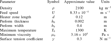
The material parameters used for one particular glass type and redraw process are shown in table 1. These parameters may vary significantly between glass types and processes.
Typical parameter values for redraw of a borosilicate glass sheet (Griffiths & Howell Reference Griffiths and Howell2008; Buellesfeld et al. Reference Buellesfeld, Lange, Biertuempfel, Pudlo and Jung2014).
2.2. Non-dimensionalization
We define two aspect ratios
 $$\begin{eqnarray}{\it\epsilon}=\frac{\text{preform thickness}}{\text{preform width}}=\frac{2h_{0}}{2b_{0}},\end{eqnarray}$$
 $$\begin{eqnarray}{\it\delta}=\frac{\text{length of heater zone}}{\text{preform half-width}}=\frac{d}{b_{0}}.\end{eqnarray}$$
 ${\it\epsilon}\ll 1$
and
 ${\it\epsilon}\ll {\it\delta}$
must be satisfied. There exist drawdown processes in which
 ${\it\delta}$
is
 $O(1)$
or indeed where
 ${\it\delta}$
is large (so the sheet is very long compared to its width). In this paper, however, we focus on industrially relevant processes where the heater zone is short relative to the sheet width, and therefore we assume that the two parameters
 ${\it\epsilon}$
and
 ${\it\delta}$
satisfy
 $$\begin{eqnarray}0<{\it\epsilon}\ll {\it\delta}\ll 1.\end{eqnarray}$$
We now non-dimensionalize the system and exploit these two small parameters by introducing
 $$\begin{eqnarray}(x^{\prime },y^{\prime },z^{\prime })=\left(\frac{x}{{\it\delta}b_{0}},\frac{y}{b_{0}},\frac{z}{{\it\epsilon}b_{0}}\right),\quad (b^{\prime },h^{\prime })=\left(\frac{b}{b_{0}},\frac{h}{{\it\epsilon}b_{0}}\right),\quad (u^{\prime },v^{\prime },w^{\prime })=\left(\frac{u}{U},\frac{v}{{\it\delta}U},\frac{w}{{\it\epsilon}U}\right),\end{eqnarray}$$
 $$\begin{eqnarray}p^{\prime }=\frac{{\it\delta}b_{0}}{{\it\mu}_{0}U}p,\quad T^{\prime }=\frac{T}{T_{0}},\quad {\it\mu}^{\prime }=\frac{{\it\mu}}{{\it\mu}_{0}}.\end{eqnarray}$$
Here
 $T_{0}$
is the maximum temperature attained by the glass inside the furnace, and
 ${\it\mu}_{0}={\it\mu}(T_{0})$
is the corresponding (minimum) viscosity. Inserting these new variables into the governing equations (2.1) and dropping the primes from the notation yields
 $$\begin{eqnarray}\displaystyle & \displaystyle u_{x}+{\it\delta}^{2}v_{y}+{\it\delta}w_{z}=0, & \displaystyle\end{eqnarray}$$
 $$\begin{eqnarray}\displaystyle & \displaystyle {\it\epsilon}^{2}(-p+2{\it\mu}u_{x})_{x}+{\it\epsilon}^{2}{\it\delta}^{2}({\it\mu}u_{y}+{\it\mu}v_{x})_{y}+({\it\delta}^{2}{\it\mu}u_{z}+{\it\epsilon}^{2}{\it\delta}{\it\mu}w_{x})_{z}=0, & \displaystyle\end{eqnarray}$$
 $$\begin{eqnarray}\displaystyle & \displaystyle {\it\epsilon}^{2}(-p+2{\it\delta}^{2}{\it\mu}v_{y})_{y}+{\it\epsilon}^{2}({\it\mu}u_{y}+{\it\mu}v_{x})_{x}+({\it\delta}^{2}{\it\mu}v_{z}+{\it\epsilon}^{2}{\it\delta}{\it\mu}w_{y})_{z}=0, & \displaystyle\end{eqnarray}$$
 $$\begin{eqnarray}\displaystyle & \displaystyle (-{\it\delta}p+2{\it\delta}^{2}{\it\mu}w_{z})_{z}+({\it\delta}{\it\mu}u_{z}+{\it\epsilon}^{2}{\it\mu}w_{x})_{x}+({\it\delta}^{3}{\it\mu}v_{z}+{\it\epsilon}^{2}{\it\delta}^{2}{\it\mu}w_{y})_{y}=0, & \displaystyle\end{eqnarray}$$
The kinematic and dynamic conditions (2.6) become
 $$\begin{eqnarray}\displaystyle & \displaystyle \pm (uh_{x}+{\it\delta}^{2}vh_{y})={\it\delta}w, & \displaystyle\end{eqnarray}$$
 $$\begin{eqnarray}\displaystyle & \displaystyle \pm {\it\epsilon}^{2}h_{x}(-p+2{\it\mu}u_{x})\pm {\it\epsilon}^{2}{\it\delta}^{2}h_{y}({\it\mu}u_{y}+{\it\mu}v_{x})={\it\delta}^{2}{\it\mu}u_{z}+{\it\epsilon}^{2}{\it\delta}{\it\mu}w_{x}, & \displaystyle\end{eqnarray}$$
 $$\begin{eqnarray}\displaystyle & \displaystyle \pm {\it\epsilon}^{2}h_{x}({\it\mu}u_{y}+{\it\mu}v_{x})\pm {\it\epsilon}^{2}h_{y}(-p+2{\it\delta}^{2}{\it\mu}v_{y})={\it\delta}^{2}{\it\mu}v_{z}+{\it\epsilon}^{2}{\it\delta}{\it\mu}w_{y}, & \displaystyle\end{eqnarray}$$
 $$\begin{eqnarray}\displaystyle & \displaystyle \pm h_{x}({\it\delta}{\it\mu}u_{z}+{\it\epsilon}^{2}{\it\mu}w_{x})\pm h_{y}({\it\delta}^{3}{\it\mu}v_{z}+{\it\epsilon}^{2}{\it\delta}^{2}{\it\mu}w_{y})=(-{\it\delta}p+2{\it\delta}^{2}{\it\mu}w_{z}), & \displaystyle\end{eqnarray}$$
 $z=\pm h(x,y,t)$
. Finally, our choice of non-dimensionalization yields the end conditions
 $$\begin{eqnarray}u(0,y,z)=h(0,y)=b(0)=1,\quad u(1,y,z)=D,\quad v(0,y,z)=v(1,y,z)=0.\end{eqnarray}$$
2.3. Thin-sheet limit
We now consider the thin-sheet limit
 ${\it\epsilon}\rightarrow 0$
, with
 ${\it\delta}$
held fixed for the moment. The details of the asymptotic analysis may be found in Howell (Reference Howell1994, Reference Howell1996) and are omitted here. The leading-order flow is found to be extensional, meaning that the in-plane velocity is uniform across the sheet, i.e.
 $$\begin{eqnarray}u=u(x,y),\quad v=v(x,y).\end{eqnarray}$$
Net conservation of mass and momentum then leads to the leading-order governing equations
 $$\begin{eqnarray}\displaystyle & \displaystyle (uh)_{x}+{\it\delta}^{2}(vh)_{y}=0, & \displaystyle\end{eqnarray}$$
 $$\begin{eqnarray}\displaystyle & \displaystyle (4\bar{{\it\mu}}hu_{x}+2{\it\delta}^{2}\bar{{\it\mu}}hv_{y})_{x}+{\it\delta}^{2}(\bar{{\it\mu}}hu_{y}+\bar{{\it\mu}}hv_{x})_{y}=0, & \displaystyle\end{eqnarray}$$
 $$\begin{eqnarray}\displaystyle & \displaystyle (\bar{{\it\mu}}hu_{y}+\bar{{\it\mu}}hv_{x})_{x}+(2\bar{{\it\mu}}hu_{x}+4{\it\delta}^{2}\bar{{\it\mu}}hv_{y})_{y}=0, & \displaystyle\end{eqnarray}$$
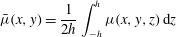 $$\begin{eqnarray}\bar{{\it\mu}}(x,y)=\frac{1}{2h}\int _{-h}^{h}{\it\mu}(x,y,z)\,\text{d}z\end{eqnarray}$$
is the viscosity averaged across the sheet thickness.
We assume symmetry about the
 $x$
-axis and hence impose the conditions
 $$\begin{eqnarray}v=u_{y}=0\quad \text{at }y=0.\end{eqnarray}$$
Net conservation of mass and momentum at the edge of the sheet lead to the boundary conditions
 $$\begin{eqnarray}{\it\delta}^{2}v=ub^{\prime }(x),\end{eqnarray}$$
 $$\begin{eqnarray}\displaystyle & \displaystyle {\it\delta}^{2}(u_{y}+v_{x})=(4u_{x}+2{\it\delta}^{2}v_{y})b^{\prime }(x), & \displaystyle\end{eqnarray}$$
 $$\begin{eqnarray}\displaystyle & \displaystyle 2u_{x}+4{\it\delta}^{2}v_{y}=(u_{y}+v_{x})b^{\prime }(x), & \displaystyle\end{eqnarray}$$
 $y=b(x)$
.
The feed and draw conditions are
 $$\begin{eqnarray}u(0,y)=h(0,y)=b(0)=1,\quad u(1,y)=D,\quad v(0,y)=v(1,y)=0.\end{eqnarray}$$
If the thickness-averaged viscosity
 $\bar{{\it\mu}}$
is a known function of
 $(x,y)$
, then the equations and boundary conditions (2.14)–(2.19) in principle provide a closed problem for the in-plane velocity
 $(u(x,y),v(x,y))$
, and the sheet half-thickness
 $h(x,y)$
and half-width
 $b(x)$
. We note that (2.14)–(2.19) are equivalent to the equations used by Filippov & Zheng (Reference Filippov and Zheng2010) to model redraw when gravity is neglected from their model.
2.4. Short heater-zone limit
We now apply the additional physically relevant asymptotic limit
 ${\it\delta}\ll 1$
, in which the heater-zone length is short relative to the preform width (but still much larger than the preform thickness), by writing the variables
 $u$
,
 $v$
,
 $h$
as asymptotic expansions in
 ${\it\delta}^{2}$
, i.e.
 $$\begin{eqnarray}{\it\psi}={\it\psi}_{0}+{\it\delta}^{2}{\it\psi}_{1}+\cdots \,.\end{eqnarray}$$
Note that the subscripts refer to an expansion in
 ${\it\delta}$
about the leading-order (in
 ${\it\epsilon}$
) solution.
In addition to our assumption that the temperature profile in the sheet is prescribed, we will restrict our consideration to temperature profiles that vary along the length of the sheet only, i.e.
 $T=T(x)$
, and
 $\bar{{\it\mu}}={\it\mu}(x)$
. This is valid provided the furnace temperature is constant in the
 $y$
-direction, with sufficiently weak coupling between flow and heat transfer. A full discussion of this assumption and the role of heat transfer in the system will be presented in § 7.
At leading order, conservation of mass (2.14a
) and
 $x$
-momentum (2.14b
) with boundary conditions (2.19) imply that the axial velocity and film thickness are independent of
 $y$
, i.e.
 $$\begin{eqnarray}u_{0}=u_{0}(x),\quad h_{0}=h_{0}(x).\end{eqnarray}$$
These functions satisfy the familiar one-dimensional model (Scheid et al. Reference Scheid, Quiligotti, Tran, Gy and Stone2009)
 $$\begin{eqnarray}\displaystyle u_{0}h_{0}=1,\quad 4\bar{{\it\mu}}h_{0}u_{0x}=1, & & \displaystyle\end{eqnarray}$$
 $$\begin{eqnarray}\displaystyle u_{0}(0)=h_{0}(0)=1,\quad u_{0}(1)=D, & & \displaystyle\end{eqnarray}$$
whose solution is
 $$\begin{eqnarray}u_{0}(x)=\exp \left(\log (D)\frac{\displaystyle \int _{0}^{x}\bar{{\it\mu}}^{-1}\text{d}s}{\displaystyle \int _{0}^{1}\bar{{\it\mu}}^{-1}\text{d}s}\right),\quad h_{0}(x)=\frac{1}{u_{0}(x)}.\end{eqnarray}$$
The
 $y$
-component of momentum conservation (2.14c
) at leading order yields an equation for
 $v_{0}$
. Integrating twice and applying homogenous Dirichlet conditions (2.19), we find that the leading-order lateral velocity is zero:
 $$\begin{eqnarray}v_{0}\equiv 0.\end{eqnarray}$$
Continuing to
 $O({\it\delta}^{2})$
, one can quickly find that the first corrections
 $u_{1}$
,
 $h_{1}$
,
 $v_{1}$
are all zero and, indeed, that all algebraic corrections are zero. Hence the leading-order outer solution (2.23), (2.24) is exponentially accurate in
 ${\it\delta}$
.
Finally, evaluating the no-flux condition (2.17) we see that
 $b(x)\sim 1$
at leading order, while the edge conditions (2.18) can only be satisfied by (2.23), (2.24) in the trivial case of no stretching (i.e.
 $D=1$
). From this result we infer that there must be a boundary layer in the region near
 $y=b(x)$
, in which a different scaling is required.
3. Boundary-layer behaviour
3.1. Rescaled problem
To satisfy the free-boundary conditions on
 $y=b(x)$
we must introduce a boundary layer at the sheet edge where the fluid behaviour changes rapidly. We therefore perform the rescaling
 $$\begin{eqnarray}b=1+{\it\delta}B,\quad y=1+{\it\delta}Y,\quad v={\it\delta}^{-1}V,\end{eqnarray}$$
so that the free surface is now located at
 $Y=B(x)$
and the outer flow (2.23) is recovered as
 $Y\rightarrow -\infty$
. The quantity
 ${\it\delta}B$
may be interpreted as the displacement of the preform edge in the
 $y$
-direction from its position at the top of the heater zone. The rescaling of the lateral velocity
 $v$
reflects the expectation that the velocity components should be comparable in the boundary layer.
The conservation laws (2.14) become
 $$\begin{eqnarray}\displaystyle & \displaystyle (uh)_{x}+(vh)_{Y}=0, & \displaystyle\end{eqnarray}$$
 $$\begin{eqnarray}\displaystyle & \displaystyle (4\bar{{\it\mu}}hu_{x}+2\bar{{\it\mu}}hV_{Y})_{x}+(\bar{{\it\mu}}hu_{Y}+\bar{{\it\mu}}hV_{x})_{Y}=0, & \displaystyle\end{eqnarray}$$
 $$\begin{eqnarray}\displaystyle & \displaystyle (\bar{{\it\mu}}hu_{Y}+\bar{{\it\mu}}hV_{x})_{x}+(2\bar{{\it\mu}}hu_{x}+4\bar{{\it\mu}}hV_{Y})_{Y}=0, & \displaystyle\end{eqnarray}$$
 $$\begin{eqnarray}u(0,Y)=h(0,Y)=1,\quad u(1,Y)=D,\quad V(0,Y)=V(1,Y)=B(0)=0,\end{eqnarray}$$
and the boundary conditions (2.17), (2.18) on the sheet edge
 $Y=B(x)$
are now given by
 $$\begin{eqnarray}\displaystyle & \displaystyle v=uB_{x}, & \displaystyle\end{eqnarray}$$
 $$\begin{eqnarray}\displaystyle & \displaystyle u_{Y}+V_{x}=(4u_{x}+2V_{Y})B_{x}, & \displaystyle\end{eqnarray}$$
 $$\begin{eqnarray}\displaystyle & \displaystyle 2u_{x}+4V_{Y}=(u_{Y}+V_{x})B_{x}. & \displaystyle\end{eqnarray}$$
This system is closed by matching to the outer solution (2.23), (2.24), i.e.
 $$\begin{eqnarray}u\rightarrow u_{0}(x),\quad V\rightarrow 0,\quad h\rightarrow 1/u_{0}(x)\quad \text{as }Y\rightarrow -\infty .\end{eqnarray}$$
The boundary-layer solutions for
 $u$
,
 $V$
and
 $h$
converge exponentially in
 $Y$
to the far-field behaviour (3.5), implying that any boundary-layer effects decay exponentially away from the sheet edges. This behaviour is consistent with our observation that the outer solution (2.23), (2.24) is exponentially accurate in
 ${\it\delta}$
.
3.2. Numerical solution
We now present numerical solutions of the boundary-layer problem (3.2)–(3.4) obtained using the finite-element software FEniCS (Logg & Wells Reference Logg and Wells2010; Logg, Wells & Hake Reference Logg, Wells and Hake2012). To enable solution with FEniCS, the domain is transformed from
 $(X,Y)\in [0,1]\times (-\infty ,B(X)]$
onto a fixed rectangle
 $[0,1]\times [-L,0]$
, with
 $L\gg 1$
; since the edge effects decay exponentially, only moderate values of
 $L$
are required to obtain accurate solutions. We use a regular triangular mesh with Lagrange elements of degree 1, and the resulting nonlinear problem is solved using a built-in Newton solver. For the case when
 ${\it\mu}=1$
and
 $D=20$
, we find that
 $300\times 260$
nodes with
 $L=3.5$
suffice to give solutions correct to two decimal places.
For the moment we focus on the case of constant viscosity
 $\bar{{\it\mu}}\equiv 1$
, so that the solution depends on a single parameter
 $D$
. A typical spatially varying viscosity profile used in industrial simulations will be considered in § 5.
In figure 4 we show the thickness profile in the boundary later for a sheet redrawn at draw ratio
 $D=20$
. As the sheet moves through the heater zone (
 $x$
increasing), we see that the cross-sectional area decreases, as expected, as the velocity increases. We also observe a departure from uniform thickness. The location of the sheet edge moves inwards and, as a result, the thickness at the edge increases relative to the bulk. In § 4 we will argue that this is a universal consequence of conservation of mass near a stress-free surface.
In figure 5 we show the velocity profile in the sheet, as well as the evolution of the sheet edge, during drawing at
 $D=20$
. Comparing figures 4 and 5 we see that the sheet necks inwards in both the
 $y$
- and
 $z$
-directions during drawing. Far from the sheet edge, the solution approaches the one-dimensional far-field behaviour (3.5), which depends only on
 $x$
, and the velocity vector points strictly in the
 $x$
-direction. However, close to the sheet edge, the velocity points inwards, and this results in the necking in of the sheet, as well as the observed difference between the edge and bulk thicknesses.
Thickness profiles inside the boundary layer for a constant-viscosity sheet drawn at a draw ratio
 $D=20$
.

Velocity profile inside the boundary layer of a sheet undergoing redraw at draw ratio
 $D=20$
under constant viscosity conditions, with free surface
 $Y=B(x)$
shown.

Finally, we ask how this behaviour depends on the draw ratio
 $D$
. Since draw resonance is not a concern, it is sensible to study (3.2)–(3.4) even for large
 $D$
. Figure 6(a) shows the final edge displacement
 $B(1)$
as a function of draw ratio; as
 $D$
increases so too does the magnitude of the change in edge position, with the rate of change decreasing for large draw ratios. Figure 6(c) shows the final sheet thickness
 $h(1,Y)$
at varying distances from the sheet edge. We observe that the difference between the edge and bulk thickness increases with increasing draw ratio. We also note the appearance of two power laws as predicted by (1.1). Far from the edge, the final thickness scales with
 $1/D$
; this corresponds to the one-dimensional behaviour described by (2.23). Close to the edge, the final thickness scales with
 $1/\sqrt{D}$
; we discuss this further in § 4. We also note that as
 $D$
grows large, small oscillations occur as the thickness profile decays away from the sheet edge; the first minimum is highlighted in figure 6(b) for a draw ratio of 80.
Dependence of sheet behaviour on draw ratio
 $D$
: (a) location of sheet edge at the bottom of the heater zone
 $B(1)$
as a function of
 $D$
, (b) final thickness profile for draw ratio 80, with a local minimum in thickness at
 $Y_{m}$
, (c) final sheet thickness as a function of
 $D$
at varying distances from the sheet edge
 $Y=B(x)$
are shown in black, while plots of
 $D^{-1}$
(dashed line) and
 $D^{-1/2}$
(dot-dashed) are shown in red.

4. Edge behaviour
We investigate the phenomenon of edge thickening in a more general setting by returning to the governing equations (2.14)–(2.19) and considering the behaviour of the fluid at the free surface
 $y=b(x)$
. Close to this free surface, it is natural to use a local curvilinear coordinate system; we let
 $s$
parametrize arc-length along the free surface and
 $n$
be the normal distance from the free surface, so that
 $$\begin{eqnarray}\tilde{\boldsymbol{x}}=({\it\delta}x,y)=s\hat{\boldsymbol{t}}+n\hat{\boldsymbol{n}},\end{eqnarray}$$
where
 $\hat{\boldsymbol{t}}$
and
 $\hat{\boldsymbol{n}}$
are the unit tangent and normal to the sheet edge. We also define tangential and normal velocity components
 $u_{s}$
and
 $u_{n}$
, respectively by
 $$\begin{eqnarray}\tilde{\boldsymbol{u}}=(u,{\it\delta}v)=u_{s}(s,n)\hat{\boldsymbol{t}}+u_{n}(s,n)\hat{\boldsymbol{n}}.\end{eqnarray}$$
The factors of
 ${\it\delta}$
in the definitions (4.1) and (4.2) account for the fact that the
 $x$
and
 $y$
variables were non-dimensionalized using different scalings.
The conservation-of-mass equation (2.14a ) may now be rewritten as
 $$\begin{eqnarray}\tilde{\boldsymbol{{\rm\nabla}}}\boldsymbol{\cdot }(h\tilde{\boldsymbol{u}})=0.\end{eqnarray}$$
In terms of the new coordinates, the kinematic boundary condition (2.17) and the normal component of the no-stress condition (2.18) at the sheet edge take the forms
 $$\begin{eqnarray}\displaystyle u_{n}=0,\quad 2\hat{\boldsymbol{n}}\boldsymbol{\cdot }[(\hat{\boldsymbol{n}}\boldsymbol{\cdot }\tilde{\boldsymbol{{\rm\nabla}}})\tilde{\boldsymbol{u}}]+\hat{\boldsymbol{t}}\boldsymbol{\cdot }[(\hat{\boldsymbol{t}}\boldsymbol{\cdot }\tilde{\boldsymbol{{\rm\nabla}}})\tilde{\boldsymbol{u}}]=0\quad \text{at }n=0. & & \displaystyle\end{eqnarray}$$
Now, by evaluating (4.3) at the free surface
 $n=0$
, and using the boundary conditions (4.4), we obtain the exact relation
 $$\begin{eqnarray}\frac{\partial }{\partial s}(h\sqrt{u_{s}})=0\quad \text{at }n=0.\end{eqnarray}$$
Thus the product of the sheet thickness and the square root of the fluid speed at the sheet edge is a conserved quantity. From the inlet conditions
 $h=u=u_{s}=1$
at
 $x=0$
, and outlet condition
 $u=u_{s}=D$
at
 $x=1$
, we deduce that the final sheet edge thickness is given by
 $$\begin{eqnarray}h(1,b(1))=1/\sqrt{D}.\end{eqnarray}$$
Dobroth & Erwin (Reference Dobroth and Erwin1986) give the following simple physical argument for this result. In the direction of drawing,
 $x$
, the elongation ratio is equal to the draw ratio
 $D$
. At the edge of the sheet there is no stress either across the sheet thickness or across the sheet width, so the elongation ratios in these directions must be the same and equal to
 $1/\sqrt{D}$
. In contrast, the outer solution (2.23) yields
 $h(1,y)\sim 1/D$
at the centre of the sheet, since the behaviour here is equivalent to that of an infinitely wide sheet, with no flow in the
 $y$
-direction. These are exactly the power-law behaviours observed in figure 6(c). It is thus clear that the final sheet thickness will always be larger at the edges than in the middle, with the disparity increasing as the draw ratio increases. Hence we provide a systematic derivation of the same power-law relationships proposed by Dobroth & Erwin (Reference Dobroth and Erwin1986) for casting of a polymer film.
It is worth emphasizing that the relation (4.6) is exact for any thin viscous sheet under tension with no stress at the edges. In contrast, the one-dimensional outer solution (2.23) is valid only in the limit
 ${\it\delta}\rightarrow 0$
, i.e. in the regime where the heater zone is short compared with the sheet width. In the regime where
 ${\it\delta}=O(1)$
, the inward retraction of the edge would affect the whole sheet and cause the thickness at the centre to be larger than the one-dimensional result
 $h\sim 1/D$
. At the other extreme, where
 ${\it\delta}\gg 1$
so the sheet is long and narrow, the edge-thickening effect would be eliminated; the sheet thickness would remain approximately uniform and scale with
 $1/\sqrt{D}$
everywhere (Howell Reference Howell1994).
5. Comparison with three-dimensional model and with redraw data
We now test the validity of our model by comparing our predictions with numerical solutions to the full three-dimensional problem (2.1)–(2.6) and with measurements from a redraw plant at Schott AG. We impose a typical dimensionless temperature profile used in industrial simulations to mimic the effects of furnace heating, namely
 $$\begin{eqnarray}T(x)={\it\theta}_{0}+(1-{\it\theta}_{0})\left(\frac{1}{1+\exp [-k(x-x_{L})]}+\frac{1}{1+\exp [k(x-x_{R})]}-1\right),\end{eqnarray}$$
where
 $x_{L}<x_{R}$
,
 ${\it\theta}_{0}<1$
and
 $k\gg 1$
are parameters. As shown in figure 7(a), the profile (5.1) remains approximately at the inlet temperature
 ${\it\theta}_{0}$
for
 $x<x_{L}$
, increases rapidly to the maximum temperature
 $T\approx 1$
for
 $x_{L}<x<x_{R}$
, then rapidly falls back to
 $T\approx {\it\theta}_{0}$
for
 $x>x_{R}$
. The parameter
 $k$
is a measure of how rapidly the transitions occur; prototypical parameter values are
 $k=20$
,
 $x_{L}=0.25$
,
 $x_{R}=0.75$
and
 ${\it\theta}_{0}=0.8$
.
A typical glass temperature–viscosity relation is of the form
 $$\begin{eqnarray}{\it\mu}=\exp \left[\frac{1}{{\it\nu}}\left(\frac{1}{T-T_{c}}-\frac{1}{1-T_{c}}\right)\right],\end{eqnarray}$$
in dimensionless variables, where
 $T_{c}$
and
 ${\it\nu}$
are parameters;
 ${\it\nu}$
is typically small so that
 ${\it\mu}$
is strongly temperature dependent. Relevant illustrative values are
 ${\it\nu}=0.1$
and
 $T_{c}=0.34$
; as illustrated in figure 7(b), this leads to a viscosity that is almost three orders of magnitude lower in the main heating zone
 $x_{L}<x<x_{R}$
than in the inlet and outlet zones.


Final thickness profile
 $h(1,y)$
at the bottom of the heater zone for a draw ratio
 $D=20$
and temperature and viscosity profiles (5.1), (5.2) with the same parameter values as in figure 7. The coloured data points are numerical solutions to the full three-dimensional Stokes problem calculated using software package Polyflow. The blue circles correspond to
 ${\it\epsilon}=0.01$
,
 ${\it\delta}=0.1$
and the red
 $\times$
symbols to
 ${\it\epsilon}=0.01$
,
 ${\it\delta}=0.2$
. The black diamonds and green crosses are the solutions to the three-dimensional Stokes problem with surface tension included (with
 $\mathit{Ca}=80$
), for
 ${\it\epsilon}=0.01$
,
 ${\it\delta}=0.1$
and
 ${\it\epsilon}=0.01$
,
 ${\it\delta}=0.2$
respectively. The data is scaled so that the profiles collapse onto the black dashed curve which is the numerical solution to the boundary-layer problem (3.2)–(3.4).

In figure 8 we show the final sheet profile calculated numerically from the dimensionless version of the full three-dimensional Stokes equations (2.1), (2.2) with associated boundary conditions (2.3)–(2.6) using the finite-element package Polyflow (Ansys Inc. Polyflow Reference Ansys Inc. Polyflow2013). We prescribe the temperature profile (5.1) on the free surface and at the inlet boundary, and the temperature in the bulk is then calculated by solving the energy equation (13.1–4 in Ansys Inc. Polyflow Reference Ansys Inc. Polyflow2013). The corresponding viscosity is then found using (5.2), as this was found to be numerically more stable than imposing the viscosity field directly in the bulk. The furnace temperature and viscosity parameters are the same as those used in figure 7. The other parameter values are
 ${\it\epsilon}=0.01$
,
 $D=20$
and two different small values of
 ${\it\delta}\in \{0.1,0.2\}$
. In all cases, the sheet was discretized using linear elements for temperature and mini-elements for velocity and pressure (for details see Fortin Reference Fortin1981; Ansys Inc. Polyflow Reference Ansys Inc. Polyflow2013). Remeshing was carried out via a streamwise method, full details of which may be found in Ansys Inc. Polyflow (Reference Ansys Inc. Polyflow2013). Grid independence was established for typical grid sizes of
 $100\times 50\times 4$
.
Figure 8 demonstrates that the scalings from (3.1) collapse the two thickness profiles onto a single curve in the neighbourhood of the edge
 $y=b(x)$
. We have also plotted the Polyflow numerical solutions to the three-dimensional problem when surface tension is included (with
 $\mathit{Ca}=80$
), and these collapse onto the same curve, verifying that surface-tension effects are not important in the inner region for this process.
In figure 8, we also plot the numerical solution to the boundary-layer problem (3.2)–(3.5), calculated using the same viscosity profile. The agreement between the full numerical solution and the boundary-layer solution is extremely good, despite the values of
 ${\it\delta}$
not being especially small. This is because we retain all of the terms in the governing equations (3.2)–(3.4) inside the boundary layer near the edge, and the influence of the free surface decays exponentially away from the edge (cf. § 2.4). The thin-sheet model surely breaks down very close to the sheet edge but nevertheless gives an excellent approximation to the thickness profile everywhere else. In summary, figure 8 demonstrates that, provided the heating zone is sufficiently short, the edge thickening effect is independent of the sheet width. The details of the thickness profile plotted in figure 8 do depend on the draw ratio and on the viscosity profile, but the asymptotic variations
 $h\sim 1/D$
in the bulk and
 $h\sim 1/\sqrt{D}$
at the edge are universal. We note a small discrepancy between the thicknesses predicted by the boundary-layer solution and by the three-dimensional solution near the sheet edge. The numerical solution of the three-dimensional problem is more challenging than the two-dimensional boundary-layer problem due to the presence of very small and large parameters, and we attribute the discrepancy to numerical error arising in Polyflow.
In figure 9, we compare numerical predictions of the final thickness profile with data from a redraw plant at Schott AG. By taking measurements with thermocouples fixed on a plate travelling through the heater zone, it was established that this heater zone corresponds to a dimensionless length of
 ${\it\delta}=0.4$
and that the induced glass temperature profile can by roughly approximated by a function of type (5.1). The blue, red and green data points indicate thickness data (measured offline using a contact profilometer) taken at three different times during typical redraw of a borosilicate glass sheet with aspect ratio
 ${\it\epsilon}=0.01$
and draw ratio
 $D=38$
. The black dashed lines show the numerical solution of the boundary-layer problem (3.2)–(3.5), while the black solid line shows the one-dimensional bulk solution (2.23). The thin pink line shows the numerical solution to the full three-dimensional problem (2.10)–(2.12).
Even for such a moderate value of
 ${\it\delta}$
, the agreement between the three-dimensional and thin-sheet models is very good. Our asymptotic solution gives an excellent prediction of the final sheet width as well as the edge and bulk thicknesses observed experimentally. However, the physical sheet is not completely flat in the bulk, and there appears to be a significant discrepancy between the predicted and measured profiles in the regions indicated by arrows in figure 9. One possible source of error is an over-simplification of the temperature profile. The two- and three-dimensional simulations assume that the temperature is a known function of
 $x$
; in reality, the temperature will vary across the sheet width (and may also vary across the thickness). A more accurate, two-dimensional temperature profile would better reflect the industrial process and improve the prediction of the thickness transition between the bulk and edge, in particular in the region highlighted in figure 9.
Thickness profile
 $h(1,y)$
at the bottom of the heater zone for a draw ratio
 $D=38$
and temperature and viscosity profiles given by (5.1) and (5.2). The blue, red and green data points show thickness profiles measured at three different times during an experimental run of the redraw process whose parameters correspond to
 ${\it\epsilon}=0.01$
and
 ${\it\delta}=0.4$
. The black dashed lines show the solution of the boundary-layer problem (3.2)–(3.4), and the black solid line in the centre, located at
 $h=1/38$
, is the one-dimensional bulk solution (2.23). The thin pink line shows the numerical solution to the full three-dimensional problem (2.10)–(2.12) calculated using Polyflow for
 ${\it\epsilon}=0.01$
and
 ${\it\delta}=0.4$
. The arrows highlight regions where the discrepancy between experimental data and the numerical solutions is significant.

6. Non-rectangular preforms
The ubiquitous edge-thickening effect demonstrated in figures 4–9 is a nuisance for glass manufacturers, and it is natural to ask whether the shape of the preform might be modified to counteract the accumulation of glass at the sheet edges. From the analysis performed in § 4, we know that the final edge thickness scales with
 $1/\sqrt{D}$
while the bulk thickness scales with
 $1/D$
. This suggests that a tapered preform whose edges have reduced thickness
 $1/\sqrt{D}$
will provide a final product with edge thickness
 $1/D$
, in line with that of the bulk of the sheet. It is not obvious, however, exactly what the shape or extent of the taper should be.
The analysis presented in this paper is valid for non-rectangular preforms, provided the preform is only doctored over a length
 $O({\it\delta})$
at the edge, i.e. provided the imposed non-uniformity is confined to the naturally occurring boundary layer. One can therefore conduct numerical experiments by solving the boundary-layer problem from § 3 with different preform thickness profiles imposed at
 $x=0$
and discover the corresponding final thickness profiles produced at
 $x=1$
; an approach similar to this was adopted by Smith & Stolle (Reference Smith and Stolle2000). Alternatively, one could impose the condition of a uniform final sheet thickness at
 $x=1$
and then try to determine the required preform profile
 $h(0,y)$
. At first glance, one would expect the resulting inverse problem to be ill posed. However, we can exploit the scaling and reflectional symmetries of the governing equations (3.2) to translate the inverse problem into a version of the forward problem already solved in § 3.
Optimal preform shape to draw a rectangular product at draw ratios 10 (green dot-dashed), 20 (blue solid) and 40 (red dashed) with constant viscosity.

The idea is to solve the boundary-layer problem (3.2)–(3.5) numerically for draw ratio
 $D=D^{\ast }<1$
. While physical compression of the sheet would certainly lead to a sinuous transverse instability, the purely in-plane thin-sheet model (3.2)–(3.5) is mathematically well posed regardless of whether
 $D$
is greater or smaller than unity. A suitable reflection and scaling of the resulting forward (starred) solution, namely
 $$\begin{eqnarray}x=1-x^{\ast },\quad h(x,Y)=D^{\ast }h^{\ast }(x^{\ast },Y),\quad u(x,Y)=\frac{1}{D^{\ast }}u^{\ast }(x^{\ast },Y),\end{eqnarray}$$
 $$\begin{eqnarray}V(x,Y)=-\frac{1}{D^{\ast }}V^{\ast }(x^{\ast },Y),\quad B(x)=B^{\ast }(x^{\ast })-B^{\ast }(1),\end{eqnarray}$$
gives a solution of the inverse problem with draw ratio
 $D=1/D^{\ast }>1$
and uniform thickness at the downstream end
 $x=1$
. Therefore, to find the optimal taper for a given draw ratio
 $D$
, we simply impose a uniform thickness at
 $x^{\ast }=0$
, solve the forward problem for draw ratio
 $1/D$
and an appropriately reflected temperature profile and record the thickness profile produced at
 $x^{\ast }=1$
. Such an ‘optimal preform’ is shown in figure 10 for three different draw ratios,
 $D=10,$
 $20,$
and
 $40$
and constant temperature and viscosity. We see that the edge thickness is
 $1/\sqrt{D}$
as expected, increasing to
 $1$
an
 $O({\it\delta})$
distance from the sheet edge.
Drawing of (a) sheet with optimal initial thickness profile, (b) sheet with linear taper, at draw ratio
 $D=20$
at constant viscosity, (c) final cross-section of tapered sheet shown in (b).

Drawing of the optimal preform at
 $D=20$
is illustrated in figure 11(a), and we see that it does indeed produce a rectangular thin sheet. While it is likely to be impractical and expensive to create a preform with a precisely specified smooth taper, it is relatively easy via a cutting process to produce a piecewise linear preform profile. The result of drawing such a linear preform is shown in figure 11(b). We see that the shape of the final product is greatly improved compared with that shown in figure 4, but that the sharp corner in the preform results in a kink in the final product as indicated by the arrow, and shown more clearly in figure 11(c). The exact inverse-problem solutions shown in figure 10 would provide a valuable guide in designing a preform shape that reduces the thickness variations in the final product while satisfying manufacturing constraints.
7. Redraw of a thin viscous sheet including fully coupled heat transfer and surface tension
The model used in this paper relies on three basic assumptions, namely that (i) inertia effects are negligible, (ii) the temperature is a known function of position in the heater zone, and (iii) surface-tension effects are negligible. The Reynolds number in industrial processes of interest is almost always small, and therefore inertia effects are indeed unlikely to be significant. However, situations may arise in which it is prudent to include coupled heat transfer and/or surface tension effects in the model. In this section we will briefly discuss the implications of each.
7.1. Heat transfer
The temperature in the glass is known a priori provided heat transfer between the glass sheet and the surrounding atmosphere is effectively instantaneous. To check this assumption, we refer to the heat transfer model outlined by Taroni et al. (Reference Taroni, Breward, Cummings and Griffiths2012) for a glass fibre, in which heat is transported within the fibre by convection, conduction and radiation, and gained from/lost to the surroundings by radiative transfer and air convection, assuming that a Rosseland approximation may be made. Taroni et al. (Reference Taroni, Breward, Cummings and Griffiths2012) find that the glass and air furnace temperatures are approximately equal provided one or both of the reduced Stanton number
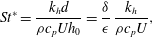 $$\begin{eqnarray}\mathit{St}^{\ast }=\frac{k_{h}d}{{\it\rho}c_{p}Uh_{0}}=\frac{{\it\delta}}{{\it\epsilon}}\,\frac{k_{h}}{{\it\rho}c_{p}U},\end{eqnarray}$$
and the parameter
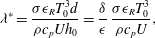 $$\begin{eqnarray}{\it\lambda}^{\ast }=\frac{{\it\sigma}{\it\epsilon}_{R}T_{0}^{3}d}{{\it\rho}c_{p}Uh_{0}}=\frac{{\it\delta}}{{\it\epsilon}}\,\frac{{\it\sigma}{\it\epsilon}_{R}T_{0}^{3}}{{\it\rho}c_{p}U},\end{eqnarray}$$
is sufficiently large. Here
 $c_{p}\approx 1000~\text{J}~\text{kg}^{-1}~\text{K}^{-1}$
is the specific heat of the glass,
 $k_{h}\approx 100~\text{W}~\text{m}^{-2}$
is the coefficient of heat transfer between the glass and surrounding atmosphere,
 ${\it\epsilon}_{R}\approx 0.9$
the specific emissivity of the glass (Taroni et al.
Reference Taroni, Breward, Cummings and Griffiths2012) while
 ${\it\sigma}=5.67\times 10^{-8}~\text{W}~\text{m}^{-2}~\text{K}^{-4}$
is the Stefan–Boltzmann constant. The parameters
 $\mathit{St}^{\ast }$
and
 ${\it\lambda}^{\ast }$
measure the effects of heat transfer from the furnace due to convection and radiation, respectively, compared with convection of heat in the glass. The representative parameter values given in table 1 imply that
 $\mathit{St}^{\ast }\approx 3.4$
and
 ${\it\lambda}^{\ast }\approx 3.8$
. While these values are sufficiently large to indicate that the heat-flow problem decouples to a first approximation, the effects of coupling may be important, especially near the edges.
Redraw is undertaken at sufficiently high temperatures that radiative heat transfer is significant. Modelling radiative heat transfer inside the sheet in full is computationally demanding, but simpler models may be developed in certain limiting cases. If the sheet is optically thick, the Rosseland approximation may be made (see, for example, Taroni et al. Reference Taroni, Breward, Cummings and Griffiths2012) and radiative heat transfer treated as a diffusion-like process. If the sheet is optically thin, and temperature variations across the sheet thickness can be neglected, a simplified model for the radiative heat transfer between the semi-transparent glass and its environment can be derived by a straightforward extension of the considerations of Modest (Reference Modest2013) on absorption, transmission and reflection of radiation in window panes.
7.2. Surface tension
The parameter values in table 1 indicate that the capillary number
 $\mathit{Ca}={\it\mu}_{0}U/{\it\gamma}\approx 80$
. Including surface tension in the model requires the imposition of a normal force on the free surface. In the thin-sheet limit the bulk momentum equations (3.2) remain unchanged, and only the boundary conditions (3.4b
) and (3.4c
) on
 $y=\pm b(x,t)$
need be modified. At the sheet edge, a force balance in dimensional terms yields
 $$\begin{eqnarray}\frac{-2{\it\gamma}}{\sqrt{1+h_{n}^{2}}}=\int _{-h}^{h}\hat{\boldsymbol{n}}\boldsymbol{\cdot }({\bf\sigma}\boldsymbol{\cdot }\hat{\boldsymbol{n}})\,\text{d}z,\end{eqnarray}$$
where
 $h_{n}=\hat{\boldsymbol{n}}\boldsymbol{\cdot }\boldsymbol{{\rm\nabla}}h$
is the normal derivative of the sheet thickness at the sheet edge. Non-dimensionalizing and integrating provides a normal stress condition
 $$\begin{eqnarray}\frac{2{\it\mu}}{1+B_{x}^{2}}[B_{x}^{2}(2u_{x}+V_{Y})-B_{x}(u_{Y}+V_{x})+(u_{x}+2V_{Y})]=-\frac{{\it\delta}}{{\it\epsilon}\mathit{Ca}}\frac{1}{h},\end{eqnarray}$$
along with the condition of zero tangential stress. These new boundary conditions could easily be incorporated into the numerical solution of the boundary-layer problem, and the presence of surface tension will act to exacerbate the problem of edge retraction. The size of the effect of
 $O({\it\delta}/({\it\epsilon}\mathit{Ca}))$
which may be
 $O(1)$
in processes of interest. However, in figure 8, we compare solutions to the full three-dimensional Stokes problem (2.10)–(2.12) with and without the inclusion of a surface tension term. The solutions are plotted in figure 8 for the cases
 ${\it\epsilon}=0.01$
,
 ${\it\delta}=0.1$
and
 ${\it\epsilon}=0.01$
,
 ${\it\delta}=0.2$
and temperature and viscosity profiles (5.1) and (5.2). We observe that the data are virtually indistinguishable and collapse onto the same curve in the boundary layer, so our assumption that surface tension may be neglected is accurate for the particular process of interest here, in which
 ${\it\delta}/({\it\epsilon}\mathit{Ca})=0.5$
.
8. Conclusions
In this paper we examine the glass redraw process, in which a prefabricated sheet is fed into a heater zone and drawn out the other end at a greater speed. We derive a mathematical model to predict how the thickness profile of the resulting final product depends on the process parameters and, in particular, to explain and quantify the anomalous thickening observed near the edges of the sheet. We find that the bulk flow is purely one-dimensional, with the axial velocity and sheet thickness satisfying the Trouton model. Variations in the sheet thickness are confined to boundary layers near the edges of the sheet, where the flow is governed by a canonical free-boundary problem. The inward displacement of the sheet edge and the local thickness profile depend on the draw ratio and on the temperature profile in the heater zone, but not on the width of the sheet. This finding should inform future manufacture of thin sheets by redraw; increasing the width of the preform while keeping the heater zone length constant will increase the yield of uniformly thin glass by the same amount, with no increase in the amount of waste due to edge thickening.
In the limit where the heater zone is very short compared with the preform width, mass conservation in the one-dimensional bulk flow implies that the ratio of final to initial bulk thickness is equal to the inverse of the draw ratio. However, the mass-conservation equation and stress-free edge conditions imply that the ratio of final to initial edge thickness is equal to the inverse square root of the draw ratio. This result holds for any thin sheet (i.e. regardless of the length of the heater zone), provided that surface tension is negligible. We thus provide a rigorous derivation of the draw-ratio relationships previously proposed by Dobroth & Erwin (Reference Dobroth and Erwin1986).
We demonstrate that the inverse problem of how to determine the optimal preform shape that will redraw to a uniform-thickness sheet may be transformed to a version of the forward problem and then solved numerically in a straightforward way. This allows us to determine the required preform that achieves a uniformly thick sheet following redraw. In addition, we predict a preform shape that achieves a final product that is close to uniform in the case where we are only able to taper the preform linearly. Here, we find that the final cross-sectional profile is close to uniform but possesses an unavoidable ‘kink’ that arises from the gradient discontinuity in the preform where the taper begins. This second result provides insight into the optimization strategy given certain preform fabrication constraints.
We may easily extend our theory to include the effect of surface tension, but doing so has little impact on the observed behaviour. We also discuss the steps for including heat transfer. In this case the modelling becomes significantly more complex as the profile evolution is coupled to temperature variations. However, including such features may be able to explain the finer details, such as the discrepancy between theory and experiment in the transition region connecting the thick edges to the main glass sheet, and the small non-uniformities observed across the sheet in the real experiment.
This work provides a novel fluid-dynamical theory that offers key insight into the redraw process, the results of which should allow for design optimization that can minimize costs and improve efficiency within the glass industry.
Acknowledgements
D.O.K. is grateful for funding from Schott AG and the Mathematical Institute, University of Oxford, and to P. E. Farrell for useful advice. I.M.G. gratefully acknowledges support from the Royal Society through a University Research Fellowship.



