BGM'S ANALYSIS OF 21 “NORTH AMERICAN INDUSTRIALIZATION PUZZLE STUDIES” (2017, P. 178)

In their Table 1, BGM calculate the change in height (between circa 1825 and 1890) in 21 anthropometric studies, and conclude that the average decline was a “trivial” 0.2 cm. However, this exercise is inappropriate for four reasons. First, the Antebellum Puzzle refers to the United States-no one has argued for a generic “North American Industrialization Puzzle” (BGM, Table 1, p. 178). Thus, the Canadian study of Cranfield and Inwood (2007) should not have been included. Second, no one suggested that everyone's height declined in the antebellum period. The consensus is that the wealthy coped successfully with the rise in relative food prices; they were able to maintain and even improve their nutritional status (Sunder Reference Sunder2011, Reference Sunder2013). Hence, studies of elite groups should not be conflated with other studies to calculate a mean change in height. Third, slaves were also special since their nutritional intake was maintained by slaveowners on efficiency wage grounds (Komlos and Coclanis Reference Komlos and Peter1997; Rees, Komlos, van Long, and Woitek Reference Haines, Lee and Thomas2003). Their heights should not be comingled with those of the free population. Thus, the five studies by Carson and two samples of Maloney and Carson (BGM p. 178), if included in the analysis, should be considered separately. This implies that in 10 of the 21 samples we would not expect to see an Antebellum decline in stature at all. Height trends in these samples depended on exceptional economic circumstances that protected particular groups from the general nutritional downturn. Without these samples, the average decline would double from BGM's 0.2 cm to 0.45 cm.

The fourth problem with this table is that for the Antebellum Puzzle, the relevant time period is the decades prior to the Civil War. BGM's results are vitiated by their periodization (1825–1890), which combines contrasting phases of economic and nutritional development (Carson Reference Sunder2011). Before the war, per capita calorie and protein availability fell as the share of the labor force in agriculture declined from 71 to 56 percent and the pace of technical improvement in agriculture was sluggish (Weiss Reference Weiss, Robert and John1992, p. 22). The post-bellum decades of Reconstruction and the early Gilded Age, instead, saw average calorie and protein intake rising again, recovering their 1840 levels by 1870 or 1880 (Floud et al. Reference Floud, Robert, Bernard and Sok2011, p. 314; Komlos Reference Komlos1987, p. 909). This was to be expected as wages in terms of food prices were increasing continuously, reaching +51 percent by 1889, and theKomlos and A-Hearn price of agricultural relative to non-agricultural products fell by 9 percent compared to 1869.Footnote ³ These were exactly the opposite of the pre-Civil War trends.

Underlying this post-bellum improvement in nutrition were developments on both the supply and demand sides. Population growth slowed considerably, even in urban areas (Haines Reference Haines, Susan, Scott, Michael, Alan, Richard and Gavin2006, Tables Aa36 and Aa46). Meanwhile, technical progress in agriculture accelerated with the diffusion of innovations such as the mechanical reaper, which proliferated beginning in the 1850s (Atack, Bateman, and Parker Reference Atack, Fred, William, Stanley and Robert2000, p. 270). By the 1870s, mechanical improvements abounded: better ploughs, seed drills, and steam- powered threshing meant the dawn of a new era in agricultural productivity. Investment in farm machinery had increased by 62 percent in the 1850s, then jumped by 275 percent between 1870 and 1900Footnote ⁴ (Olmstead and Rhode Reference Olmstead, Paul, Susan, Scott and Michael2006, Tables Da24 and Da25). Consequently, total factor productivity growth in agriculture more than doubled, from 0.36 percent in the 1830s and 0.18 percent in the 1840s to 0.77 percent across the whole second half of the nineteenth century (Atack, Bateman, and Parker Reference Atack, Fred, William, Stanley and Robert2000, p. 259).

Of particular relevance for protein availability, average milk yields per cow increased by 40 percent during the second half of the century, and refrigerated railroad cars were making their debut, facilitating the transport of perishables over longer distances (Craig, Goodwin, and Grennes Reference Craig, Goodwin and Thomas2004; Atack, Bateman, and Parker Reference Atack, Fred, William, Stanley and Robert2000, p. 260). Meanwhile, public health measures including sewage treatment, canalization, and running water provision began to improve the epidemiological environment (Craig Reference Craig, John and Inas2016). As we would expect in a period of increasingly abundant calories and protein, and decreasingly virulent disease, the post-bellum decades saw the decline in stature reversed. By the Gilded Age, the uptick in heights was well underway.

BGM's inappropriate periodization also causes them to omit 13 important studies which form the cornerstone of the evidence for the Puzzle, but do not extend to 1890 (A'Hearn Reference A'Hearn, John and Joerg1998; Bodenhorn Reference Bodenhorn1999; Cuff Reference Cuff2005; Haines Reference Haines, John and Joerg1998; Haines, Craig, and Weiss Reference Haines, Lee and Thomas2003; Komlos Reference Komlos, Claudia and Hugh1992; Komlos and Coclanis Reference Komlos and Peter1997; Komlos and A'Hearn Reference Komlos and Brian2016; Lang and Sunder Reference Lang and Marco2003; Margo and Steckel Reference Margo and Richard1983; Steckel Reference Steckel1995; Sunder Reference Sunder2004; Yoo Reference Yoo2012). Thus, BGM's 21 samples are selected in such a way that they are unrepresentative of the anthropometric history of the antebellum period.

Their justification for the 1825–1890 periodization appeals to “Fogel's (1986) account” of height trends, which they believe has “achieved nearly iconic status” (BGM 2017, p. 176). But Fogel's 30-year old “account” was a simple back-of-the-envelope guesstimate: it was not based on actual national data. Instead, it filled a gap in the national height series with the heights of Ohio National Guardsmen. Fogel not only assumed that heights at the national level moved as did heights in Ohio, which had no evidential basis, but also had to guess the level at which to splice the two series together. Apparently BGM did not take seriously Komlos' warning that “the decline in heights during the period of post-Civil War Reconstruction was shallower than the one based on interpolation from the Ohio National Guard” and that “the difference between the interpolated and actually estimated results was a full inch (2012, pp. 407, 441).” Since 1986, new evidence has emerged: Zehetmayer's study based on actual national data indicated that the decline in heights continued into the 1850s but was over by the 1860s. Heights stagnated through the 1870s and then began to rise, increasing some 0.4 inches (1 cm) by the 1890s (Zehetmayer Reference Zehetmayer2011, pp. 318, 320, 322; Komlos Reference Komlos2012, p. 442; Craig Reference Craig, John and Inas2016, p. 756). Hence, the Antebellum Puzzle was over by the 1860s. Zimran comes to the same conclusion: the diminution of heights was over by the Civil War (2019, p. 128). In the light of recent research, then, the consensus is that the Antebellum Puzzle pertains exclusively to the antebellum decades. Iconic or not, Fogel's 1986 conjecture has been superseded. Not only the choice of samples included in BGM's Table 1 but also their conflation of the antebellum decades with Reconstruction and the Gilded Age irreparably biases the results.

BGM'S TABLE 5 DOES NOT SUPPORT THEIR CONTENTION

We replicate BGM's analysis of the Union Army data in their Table 5 (2017, p. 198). Following BGM, we select U.S.-born soldiers aged 23-30, although there is no compelling reason to exclude from the analysis adults up to age 45 (the Army regulation maximum); this reduces the number of observations from 11,749 to 7,458.Footnote ⁵ In selecting the sample and determining birth-year, we use the age declared by the recruit at the time of enlistment.

BGM explore selection effects in a regression framework. As a baseline, they estimate a simple model of height as a function of birth year:

(1) \begin{equation} $${{h}_{bi}}=\alpha +\sum{_{b=1832}^{1842}}{{\beta }_{b}}\cdot {{d}_{bih}}+{{\varepsilon }_{i}},$$ \end{equation}

where h_bi is the height of soldier i, born in year b; d_b is a dummy for birth in year b; the constant α refers to a soldier born in 1831; and ε_i is a random disturbance.Footnote ⁶ The estimated birth-year effects $\left( {{{\hat \beta }_b}} \right)$ are highly statistically significant, and indicate a large decline in heights of ca. 1.5 inches (3.8 cm). BGM plot these estimates as a long-dashed line in their Figure 3.

Figure 1

MEAN HEIGHT BY BIRTH- AND ENLISTMENT-YEAR IN THE BGM SAMPLE OF UNION ARMY SOLDIERS AGED 23–30

Note: Difference in predicted mean height (inches) relative to 1831 birth and 1861 enlistment derived from RSML estimates of the Equation (2) (Model 4).

Source: Our estimate using the data in Fogel et al. (Reference Fogel, Stanley, Clayne and Larry1990).

To the basic model of Equation (1), they add variables which should not matter in the absence of selection effects: dummies for ages 24–30 (Models 1 and 3), dummies for enlistment-years 1862–1865 (Models 2 and 4), interactions between age and enlistment-year (Model 3), and interactions of birth-year and enlistment-year (Model 4). Hypothesis tests based on these models are reported in Column (1) of our Table 1 (and BGM's Table 5). For instance, the specification of Model 4 is:

(2) \begin{equation} $$\eqalign{& {h_{bei}} = \alpha + \sum {_{b = 1832}^{1842}} {\beta _b} \cdot {d_{bi}} + \sum {_{e = 1862}^{1865}} {\gamma _e} \cdot {d_{ei}}\\ & \,\,\,\,\,\,\,\,\,\,\,\,\,\,\,\, + \sum {_b\sum {_e{\delta _{be}}} \cdot {d_{bi}} \cdot {d_{ei}} + {\varepsilon _i}.}} $$ \end{equation}

In addition to birth-year dummies, Equation (2) includes enlistment-year dummies (d_e) that allow the level of heights to differ by enlistment year, and a set of (d_b · d_e) interactions that allow height trends to differ by enlistment year.Footnote ⁷ In the absence of varying selection effects, neither enlistment-year nor the interaction between enlistment-year and birth-year should have predictive power. Those born in 1840 who enlisted in 1863 at age 23, for example, should have the same mean height as those born in 1840 who enlisted in 1864 at age 24. Hence, statistically significant effects of these “selection variables” would be suggestive of changing selection effects.Footnote ⁸

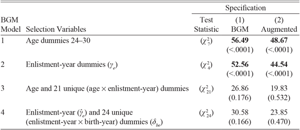
The χ² statistics and p-values reported in Column (1) of our Table 1 (BGM's Table 5, Column (1)) pertain to tests of the joint significance of the selection variables in each regression model. Birth-year effects are included in all models and are not the subject of the reported statistical tests. Our results are almost identical to theirs and confirm that age or enlistment- year dummies are, indeed, statistically significant in Models 1 and 2, which BGM consider evidence of selection effects: “These diagnostic tests reveal a troubling pattern: in almost all samples, individuals within the same birth cohort who enter the military at different ages have different mean height by age at enlistment (or, equivalently, by enlistment year). Since we only examine ages after reaching full-height, this is prima facie evidence of height-based selection into the military” (BGM 2017, p. 202).

We agree, except that these results are not “troubling.” Consider Model 2, estimates of which indicate that men born in a given year but recruited later in the war were shorter. There exist variations in mean stature so subtle as to be perceptible only in large datasets using modern computing power, but this is not one of them. Contemporaries were well aware that the average heights of new recruits decreased over the course of the conflict. In 1869, in the immediate aftermath of the war, Gould noted “a decided tendency to diminution of the average stature as the war went on” (1869, p. 92). From the beginning, anthropometric historians realized that it was necessary to control for enlistment-year. Margo and Steckel confirmed that the height of soldiers at the end of the war was 2 cm (0.79 inches) shorter on average than those who enlisted at the beginning (1983, p. 170). A'Hearn (1998, p. 265) and BGM (2017, pp. 191, 199) estimate an effect of similar magnitude. Thus, there was increasingly negative selection on height during the war. So long as this operated equally, within a given enlistment-year, on men of all birth-years, controlling for enlistment-year allows us to estimate the time trend in heights accurately. This has been the standard practice.

Table 1

TESTING FOR SELECTION (CF. BGM TABLE 5)

Notes: Birth-year is an explanatory variable in all four models Models 1–4 add different selection variables: Model 1 adds age dummies; Model 2 adds enlistment-year dummies for 1862–1865; Model 3 adds both age and age by enlistment-year interactions; Model 4 adds both enlistment-year and birth-year by enlistment-year interactions. Column (1) uses BGM's specification; Column (2) includes birth-region and occupation as additional controls. The table presents chi-square test statistics and associated p-values (in parentheses) for the hypothesis that the coefficients on the selection variables specified in each row (excluding birth-year) are jointly zero. Significant coefficients are shown in bold. Sample size = 7,458.

Source: Our RSML estimates based on data in Fogel et al. 1990.

Model 1, in which height is a function of birth-year and age, shows us the enlistment-year effect from a different perspective. Birth-year, enlistment-year, and age are perfectly collinear: every man born in 1838 enlisting in 1861, for example, was exactly 23 years old.Footnote ⁹ We can either ask whether the mean height of the 1838 birth cohort differed in 1862, 1863, 1864, and 1865, or whether it differed at age 24, 25, 26, and 27. If there was increasingly negative selection on height in successive enlistment years, a fact about which everyone agrees, we must find that men of a given birth-year were on average shorter at older ages. Hence, Model 1 's age effects and the decline in height-by-age depicted in BGM's Figure 2 are the long-understood enlistment-year effects viewed from a different angle.

Figure 2

ALTERNATIVE ESTIMATES OF BIRTH-COHORT EFFECTS

Note: RSML estimates of β_b in Equation (2) (Model 4). Both sets of estimates omit 16 of the possible birth-year/enlistment-year (b × e) interactions. The “base '65” series follows BGM in setting e =1865 as the reference, omitting all its interactions. Estimates labeled “base 64” instead have e =1864 as the baseline. Both estimates additionally omit the first and last birth-year for the non-reference enlistment-years. Markers on the “base '64” line indicate statistical significance at 5 percent.

Source: Our estimates using the data in Fogel et al. (Reference Fogel, Stanley, Clayne and Larry1990).

The interaction effects tested in Models 3 and 4 allow for the kind of selection that would create serious problems for estimating historical height trends: differential selection on height by birth-year, within a given enlistment-year (or age). Such variable selection would bias estimates of the trend in heights even with enlistment-year controls. But BGM do not find these interaction effects jointly statistically significant. Nor do they make any claim that they are meaningfully large. We, too, find that the interactions are insignificant. So, there is no evidence at all that selection operated differently on different birth-years (ages) within enlistment-years. The interaction terms do not matter: the enlistment- year effect operates uniformly on all birth-years, so that trend estimates are not distorted.

To be sure, BGM do report statistical significance in Column (2) of their Table 5, a result we can reproduce. But in this case, they are using an inaccurate measure of age (and with it, birth-year). This alternative measure of age was reported decades later, when a veteran applied for a pension. The accuracy of this measure is undermined by both survival bias and monetary incentives to overstate age, since beginning in 1890 pensions were available for veterans over 65 even if they were not disabled.Footnote ¹⁰ Meanwhile, BGM's Column (3) results are estimated from a small subsample with accurate ages: those cases in which the age or birth-year reported at enlistment and in a pension application coincide.Footnote ¹¹ Here again they (and we) find no evidence of statistically significant interaction effects.

A weakness in BGM's analysis is their failure to control for region of birth or occupation, when we know sample composition varied across enlistment years. For example, the share of farmers in the estimating sample was 41 percent in 1861 but 57 percent in 1862, while the share born in New England declined steadily from 13 percent in 1861 to just 3 percent by 1865. We include these additional controls in the four regressions reported in Column (2) of our Table 1. We find that the interactions in Models 3 and 4 are now even less significant than in Column (1); the p-values increase by a factor of three, further weakening any support for BGM's argument.

In sum, neither BGM's Figure 2 nor Table 5 support their argument. Their Figure 2 and the tests of Models 1 and 2 in their Table 5 reflect well-known enlistment-year effects, which have been controlled for in the literature. And they fail to find significant interaction effects in Models 3 and 4 when using accurate birth-year and age information (Columns (1) and (3) in their Table 5). The significant enlistment-year effects are evidence of selection and do matter for the level of the height estimates, but there is no evidence that the trend in heights is distorted. The Antebellum Puzzle passes the χ² tests.

BGM'S FIGURE 3 IS MISLEADING

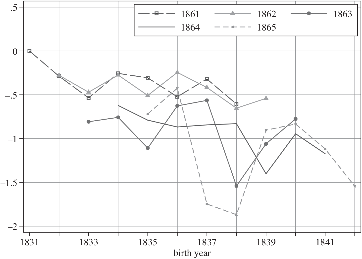
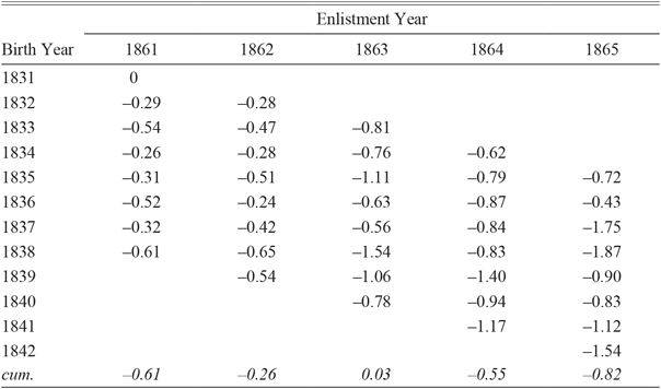
The estimates of Equation (2) (Model 4) can be understood best when presented graphically as in Figure 1. The points there represent predicted mean height for soldiers born in a given birth-year (b) and enlisting in a given year of the war (e): ${\hat h_{be}} = {\hat \beta _b} + {\hat \gamma _e} + {\hat \delta _{be}}$ The numerical estimates are presented in Table 2. By omitting the constant α we express mean heights as differences relative to the reference group: soldiers born in 1831 and enlisting in 1861. We join the points pertaining to a given enlistment-year with a line to illustrate trends for each of the enlistment years.

Table 2

MEAN HEIGHT DIFFERENCES RELATIVE TO BIRTH-YEAR 1831

Note: RSML estimates of mean height of soldiers in inches relative to a reference of birth-year (b) 1831 and enlistment-year (e) 1861, calculated as ${\hat \beta _b} + {\hat \gamma _e} + {\hat \delta _{be}}$. These values are plotted in Figure 1. The row labeled “cum.” (for cumulative) gives the change in mean height between the first and last birth-year observed for a given enlistment-year.

Source: Our estimates of Equation (2) using the data in Fogel et al. 1990.

The hypothesis test in our Table 1, Model 2, implies that enlistment-year effects (the ${\hat \gamma _e}{\rm{s}}$) are highly statistically significant. We can see in Figure 1 that they were also quantitatively important. Soldiers of the same birth cohort who enlisted later in the war (1863–1865) were shorter by anywhere from a quarter- to a full-inch, compared with the men who signed up earlier. This is evidence of changing selection on height, and failure to control for it would seriously bias any attempt to infer population heights from military heights. Not only the level, but also the trend would be affected, since the final birth-years are observed only in the later enlistment-years.

The hypothesis test in our Table 1, Model 4, implies that birth-byenlistment-year interaction effects (the ${\hat \delta _{be}}{\rm{s}}$) are not statistically significant when accurate birth-year estimates are used. We see in Figure 1 that they are not quantitatively important either. Within each enlistment-year, mean heights fall for progressively later-born soldiers. These falls range from −0.26” to −0.82”, as the bottom row of Table 2 shows, and are statistically significant.Footnote ¹² The recruits of 1863 are an exception, but the estimating sample in this case is relatively small (just 426 observations), so one should not be too concerned about that.Footnote ¹³ Clearly, a systematic tendency is observable in Figure 1. There is no evidence that the varying annual fluctuations around the trends are anything other than random sampling-induced noise. So, the data, by formal hypothesis test and by informed judgment, support Model 2, not Model 4. And the ${\hat \beta _b}{\rm{s}}$ for Model 2 (not reported here) indicate a statistically significant fall in heights of −0.92 inches from 1831 to 1842.

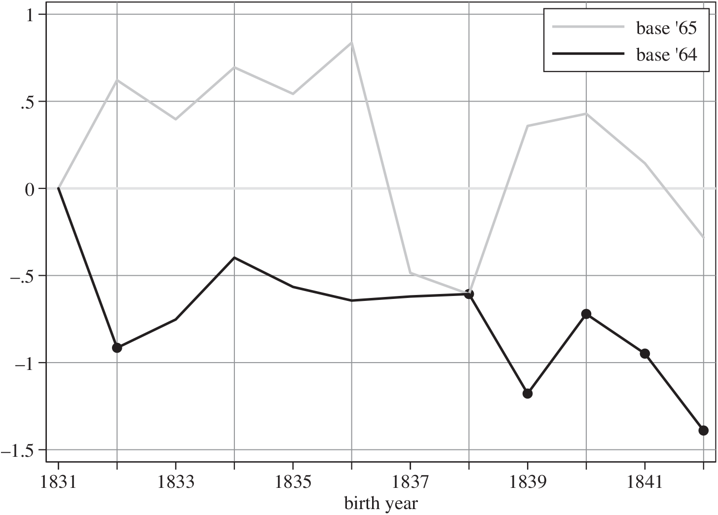
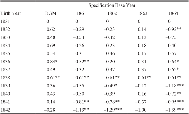
However, BGM's Figure 3 (solid line) creates a very different impression, showing nothing like a steady decline. The authors emphasize this, commenting that “the standard error bands imply that we cannot reject the null of no change in height” (p. 196). But what BGM's Figure 3 is actually showing is not transparent. Its title is “Birth-cohort and Recruit- year controls: RSMLE estimates” which is rather opaque (RSMLE stands for reduced sample maximum likelihood estimator). What their solid line in fact plots are estimates of β_b from Model 4. At first glance, this seems an intuitive representation of the trend in heights; the β_bs are birth-cohort effects, after all, and we have just described the ${\hat \beta _b}{\rm{s}}$ of Model 2 as a valid estimate of the trend in heights. There are two problems with the ${\hat \beta _b}{\rm{s}}$ of Model 4. First, they are noisy due to overfitting: BGM estimate 40 parameters from 40 observed (e × b) combinations, such that the estimates are picking up random variation in the data. Second, they are not invariant to the choice of which interactions to omit when estimating the model. This last difficulty is technical, but not just a technicality.

Model 4 predicts mean height for the 40 combinations of birth-year and enlistment-year observed in the sample (those in Table 2). BGM estimate 11 birth-year (b) and four enlistment-year (e) main effects relative to a reference group. Including the constant, that makes 16 parameters, meaning only 24 of the possible 40 (b × e) interaction effects can be estimated; 16 must be omitted. The choice of which 16 to omit is arbitrary and makes no difference to the predicted mean heights we plot in Figure 1, nor for the test statistic regarding the joint significance of the interactions in Table 1. It does make a difference for the estimates of β_b considered on their own.

BGM set the reference enlistment-year as 1865, thus omitting the eight (b × e) interactions involving e = 1865; they further omit the first and last birth-year for each of the other four enlistment-years. That yields the ${\hat \beta _b}{\rm{s}}$ in their Figure 3 (solid line), which we reproduce in Figure 2. What happens if we introduce an innocuous change, making 1864 the reference enlistment-year, thus omitting the eight e = 1864 interactions instead of those involving 1865, but leaving everything else the same? The “base '64” line in Figure 2 shows that the ${\hat \beta _b}{\rm{s}}$ now fall from 1831 onwards, reaching −1.4 inches in 1842. The estimates for birth-years 1838–1842 are all statistically significant at the 5 percent level. Alternative choices of omitted interactions produce still more ${\hat \beta _b}$ trajectories, a few of which are presented in Table 3. None is better than the others. They are all wrong, in a sense, inasmuch as the ${\hat \beta _b}{\rm{s}}$ in Model 4 are estimated jointly with the ${\hat \delta _{be}}{\rm{s}}$ and these latter are picking up random noise rather than effectively controlling for selection effects. A fuller analysis of the betas with different base years is found in Online Appendix B. BGM's Figure 3 is thus seriously misleading: the line is not a representative trend in height.

Table 3

ALTERNATIVE ESTIMATES OF BIRTH-YEAR EFFECTS (β_b)

* = Significant at the 10 percent level.

** = Significant at the 5 percent level.

*** = Significant at the 1 percent level.

Note: RSML estimates of birth-year effects (β_b) in Equation (2) (Model 4), when different interaction variables (d_b · d_e) are excluded from the estimating equation. BGM omit interactions involving the first and last birth-year (b) observed for each enlistment year (e), plus all interactions involving e =1865. The specifications labeled 1861-1864 follow the same pattern regarding first and last birth-years, additionally dropping all interactions with e =1861, 1862, 1863, and 1864, respectively.

Source: Our estimates of Equation (2) using the data in Fogel et al. Reference Fogel, Stanley, Clayne and Larry1990.

REAL TRENDS IN HEIGHT

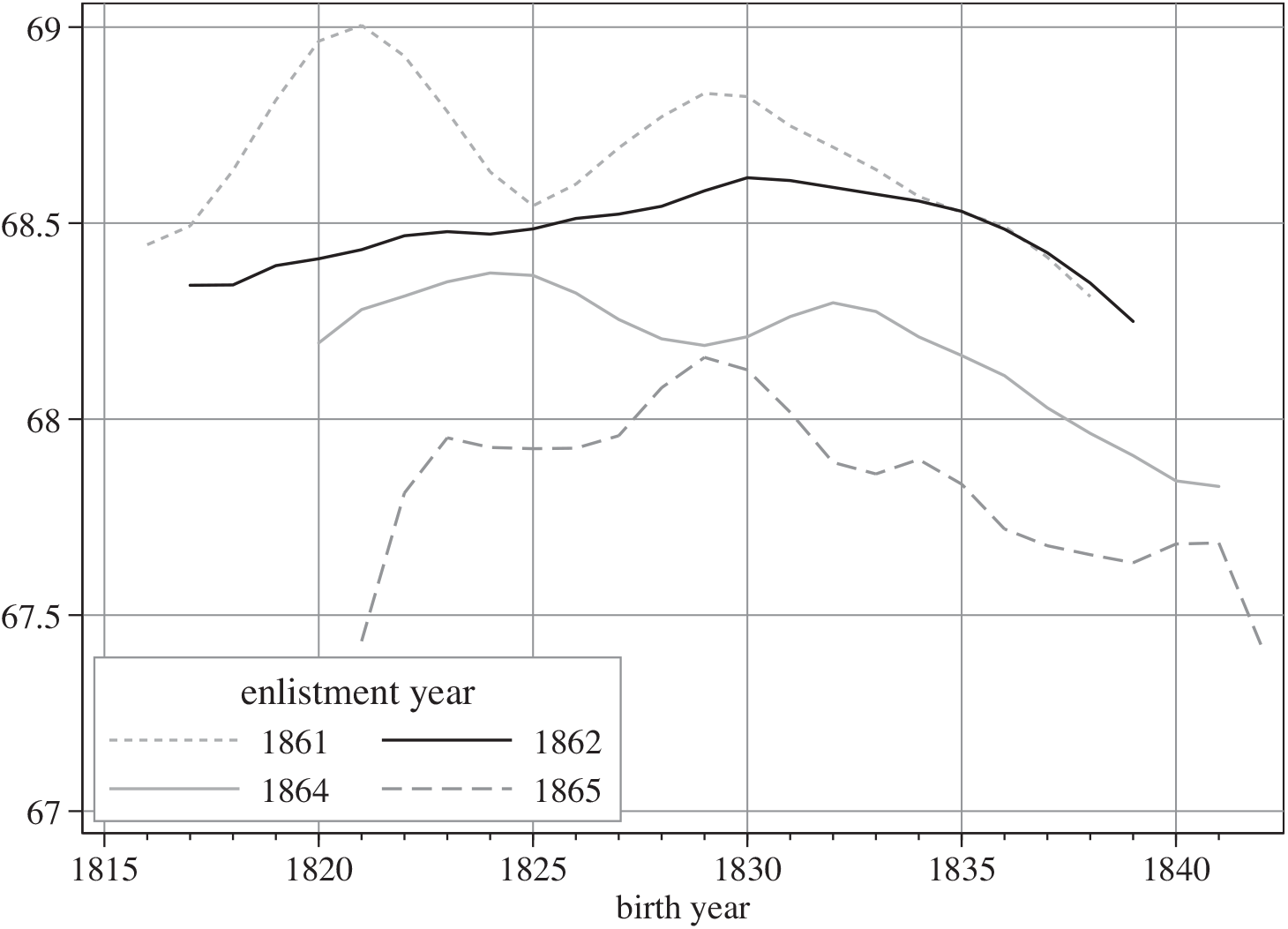
We extend the analysis by expanding the working sample to include soldiers aged up to 45 thereby increasing the sample from 7,458 to 11,749 observations.Footnote ¹⁴ Moreover, we include the explanatory variables birthregion and occupation to control for fluctuations in sample composition. By considering recruiting periods as short as 90 days, we effectively hold labor market conditions and associated selection pressures constant.

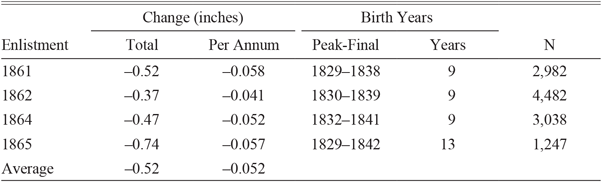
Figure 3 shows the new estimates of mean stature trends by enlistment year (with annual figures smoothed for ease of visualization). Consistent with the results presented earlier, men recruited later in the war were shorter. This effect, due to recruits being drawn from lower social strata and known since 1869, does not distort the trend estimated within an enlistment year. In every case, within enlistment-year trends indicate declining stature among the birth cohorts of the 1830s and early 1840s.Footnote ¹⁵ As set out in Table 4, the declines from peaks near 1830 to the final observed birth-year are remarkably similar, with an average of about −0.05 inches (0.13 cm) per annum or −0.52 inch (1.3 cm) per decade. The average decline in heights during the period considered was around 0.52 inches (Table 4). Zehetmayer documents another 0.38 inches decline in the 1850s and 1860s. That implies that the total decline in the antebellum decades was probably near 0.9 inches (2.3 cm).

Figure 3

REAL HEIGHT TRENDS BY ENLISTMENT YEAR

Notes: Predicted mean heights from an estimate of Equation (2) (Model 4), extended to cover ages 23-45 and including controls for birth-region and occupational group. The reference group are New England-born farmers born in 1831 and enlisting in 1861. Estimation is by RSMLE with lower truncation points of 64.5” (to 31.08.1861), 63” (31.08.61 - 31.12.1864), and 60” (throughout 1865). The interaction effects are not jointly statistically significant. The annual mean height estimates have been smoothed by locally weighted regression. Sample sizes by enlistment year are 2,982, 4,482, 655, 3,038, and 1,247, for a total of 12,404. (The small sample for 1863 results in volatile, imprecise estimates which we have not plotted. The 1863 estimates show heights falling roughly half an inch from the mid-1820s to the late 1830s.)

Source: Our estimates using the data in Fogel et al. (Reference Fogel, Stanley, Clayne and Larry1990).

Table 4

DECLINE IN MEAN HEIGHT BY ENLISTMENT YEAR OF RECRUITS 23–45 YEARS OLD

Note: Based on predicted mean height, ${\hat \beta _b} + {\hat \gamma _e} + {\hat \delta _{be}}$, from an RSML estimate of Equation (2), modified to accommodate birth-years 1816–1842. Declines measured from the local peak nearest to 1830 in the smoothed annual series to the final birth-year observed, as specified in the “peakfinal” column. Figures reported in the bottom row are simple averages of the figures computed separately for each enlistment year. Enlistment-year 1863 was included in the estimating sample, but with only 655 observations produced volatile, imprecise estimates.

Source: Our analysis of the data in Fogel et al. 1990.

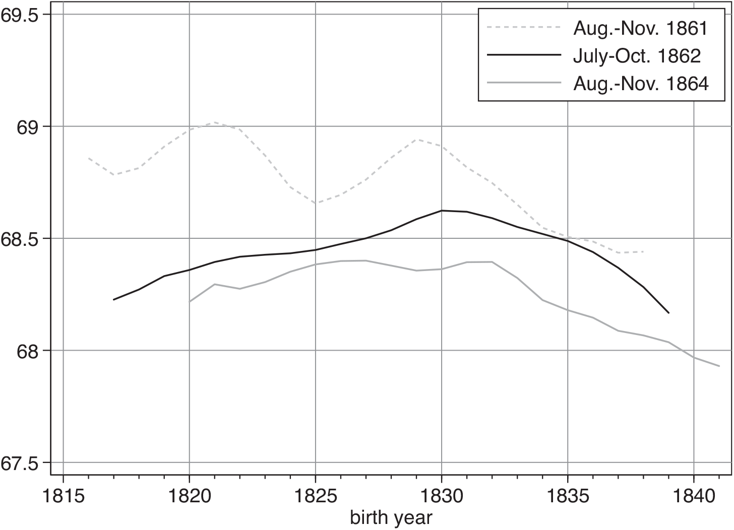
In addition, we can identify three 90-day recruitment windows with sufficient observations to permit accurate trend estimates (Figure 4). Two of these (August–November 1861, and July–October 1862) are from the period before conscription was introduced and one after (August–November 1864). Sample sizes are 1,684, 3,477, and 1,240, respectively. The downward trend in height after 1830 is unmistakable in all three cases. The difference in mean heights at the end of the series relative to 1831 birth is statistically significant and in the range of 0.4 – 0.8 inches. These periods are so short that changing self-selection due to changing labor market conditions cannot have been of any significance.

Figure 4

REAL HEIGHT TRENDS BY 90-DAY ENLISTMENT WINDOWS

Note: Smoothed annual estimates of predicted mean height by birth-year from separate regressions on samples drawn from the 90-day recruiting windows indicated in the legend. Height was regressed on dummies for birth-year, birth-region, and occupational group. Estimation method, truncation points, and smoothing technique as in the note to Figure 3.

Source: Our estimates using data in Fogel et al. (Reference Fogel, Stanley, Clayne and Larry1990).

HISTORICAL EVIDENCE ON RECRUITMENT, WAGES, AND SELF-SELECTION

BGM argue that the decline in sample heights of the Union Army soldiers is not indicative of population trends, since men were motivated by market incentives to self-select into military service. This model of self-selection into occupations was first proposed by Roy (1951). BGM assert that as business conditions improved, more productive taller men chose to work in the private sector instead of the military with the consequence that shorter men entered the military in good times: “improvements in civilian labor markets would lead to a shorter army (2017, p. 201).” However, this simple version of the Roy model is not applicable to the military in wartime; it was not conceived for situations in which survival itself was uncertain and non-pecuniary factors—such as patriotism—were decisive. In the Online Appendix A we consider historical evidence on economic incentives to enlist, the motivations of volunteers, recruitment practices, and the socioeconomic status of soldiers as they evolved over the war.

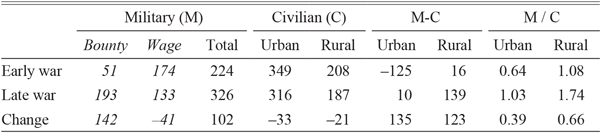
Throughout the first phase of the war, economic incentives to enlist were weak at best. The army paid privates just $13 per month, at a time when the wage of unskilled labor was about a dollar a day. Even a federal enlistment bounty of $100 failed to make this competitive with civilian incomes. Annual military compensation was about $125 less than urban wages even including the value of rations, and roughly equal to rural wages (Table 5). Given the uncertainty and hardship of military life, there was no meaningful incentive to self-select into the military on pecuniary considerations. Patriotism made up the difference.

Table 5

CIVILIAN AND MILITARY PAY (1860 DOLLARS)

Note: All figures on an annual equivalent basis over the term of service, in constant 1860 dollars. M-C is the military-civilian gap in dollars; M/C is the military-civilian compensation ratio. Source: Wage and bounties from supplementary tables to Lewis and Goldin (Reference Goldin and Frank1975). Further detail on calculations and sources in Komlos and A'Hearn (Reference Komlos and Brian2016), Online Appendix B.

The Enrollment Act of March 1863 marked a turning point in recruitment. The Act established Federal conscription for the first time, although also allowing drafted men to furnish a substitute (or, initially, pay a commutation fee of $300). In the aftermath of the infamous draft riots in the summer of 1863, New York City began paying $300 to drafted men to enable them to pay commutation or pay a substitute. In October 1863 the Federal enlistment bounty was tripled to $300 (even more for re-enlisting veterans). As Table 5 shows, wartime inflation eroded the real value of both military and civilian wages, but in the case of the army this was more than offset by a near quadrupling of enlistment bounties. There is no mistaking the direction of change: military service became economically more attractive over time rather than less so. This is exactly the opposite of what would be required to generate a spurious downward trend in heights as BGM suppose based on the Roy model. If pecuniary considerations had been utmost in men's minds, the model predicts that the military option should have become more attractive and taller men should have enlisted as the war persisted. Instead, as total military compensation rose relative to civilian wages, from 64 to 103 percent in cities and from 108 to 174 percent in rural areas, military heights declined, instead of increasing.Footnote ¹⁶

The historical record indicates that initially patriotism overwhelmed economic considerations, such that men from all strata enlisted, including many educated, middle-class, and even upper-class men who are usually taller than average.Footnote ¹⁷ A similar pattern had been observed in the Mexican–American War. An 1856 government report compared the soldiers of the Regular Army unfavorably with the volunteers who flocked to the colors at the outbreak of the war. The former were “not of the most desirable character” because there was “little inducement to enter a service where the pay is small, and the duties both arduous and dangerous.” The wartime volunteers, instead, “were taller, more intelligent, had better constitutions and habits, and were for the most part young and enthusiastic… These men were mostly actuated either by motives of patriotism, or by the desire for change and excitement, and not by the hope of pecuniary reward” (Coolidge Reference Coolidge1856, pp. 625–28). The same considerations applied a fortiori to the Civil War. Only as the fighting dragged on and the casualties mounted did patriotic passions cool, such that a larger share of the soldiers came from the lower ranks of the society, men who were shorter even controlling for region and occupation. This is what the estimates of enlistment-year effects are capturing. However, such uniformly negative selection, affecting all men enlisting in a particular year, does not distort estimates of the time trend in heights since the decline is uniform across birth years.

FURTHER EVIDENCE ON SELF-SELECTION BY AGE

Thus far we have followed BGM in focusing on changing labor market conditions over time as a potential cause of spurious trends. An alternative mechanism could operate through differential selection by age, for example, if in every recruitment period taller-than-average 30-year-olds self-selected into the military but shorter-than-average 23-year-olds enlisted. Yet, the logic of the Roy model suggests just the opposite. It is surely not a stretch to imagine upward-sloping age-earnings profiles in civilian labor markets in antebellum America, driven by physical maturation, investment in skills, and sorting into jobs best-matched to aptitudes. Given that military pay was the same for all enlisted men, the opportunity cost of military service would thus have been higher for older men. Moreover, older men were more likely to be married, to have a family dependent on their incomes, and to have farms or businesses requiring their ongoing management. Only the least-skilled, lowest-earning (and thus on average shorter) older men should have found the army economically attractive.

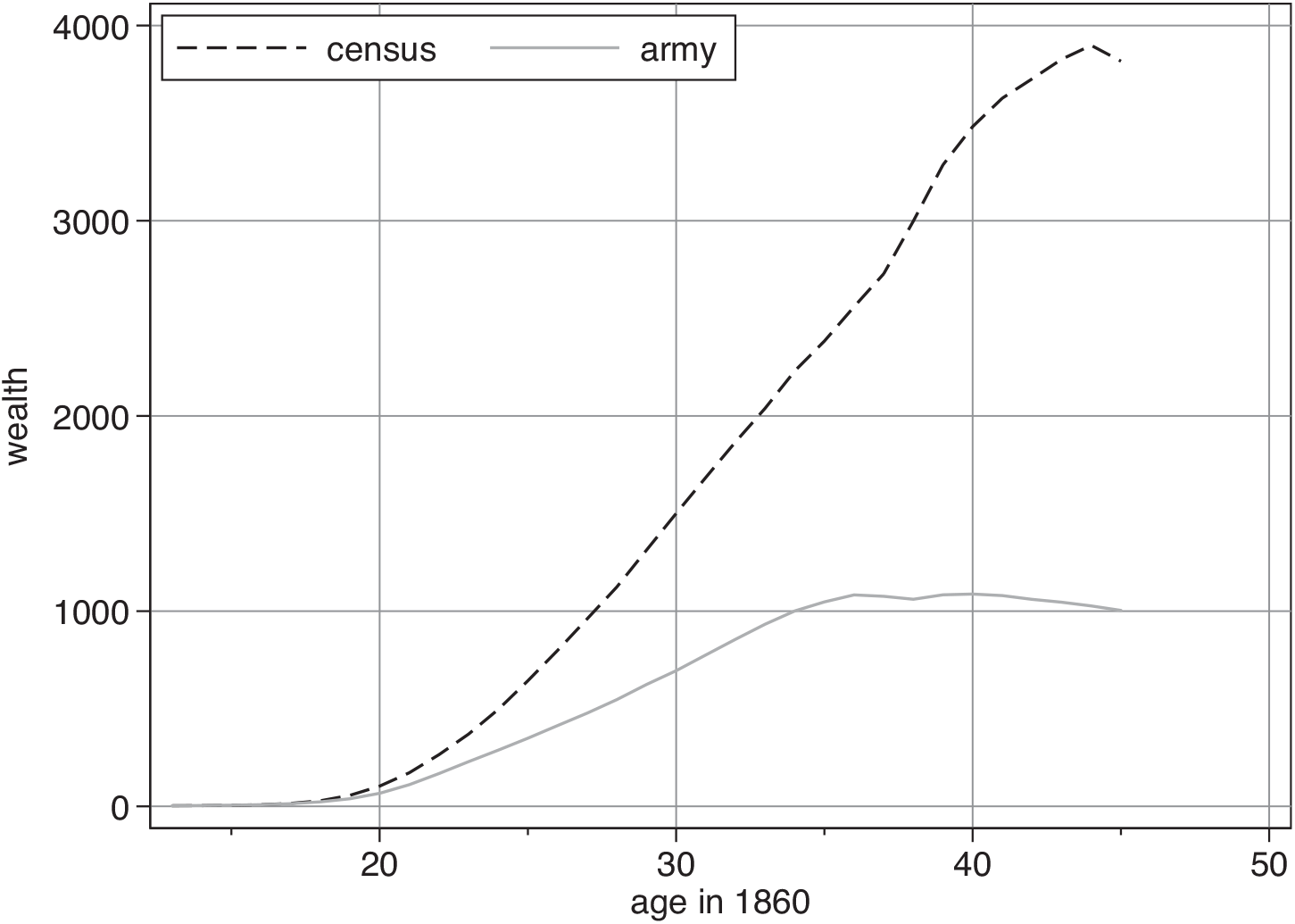
Nor does a review of detailed, local studies of Civil War recruitment yield any evidence of age-related self-selection that would have brought the “best” of the older generation and the “worst” of the younger generation into the army (see the Online Appendix A for elaboration). And there is empirical evidence against such a pattern. The Early Indicators Project successfully linked 40 percent of soldiers to the 1860 census, which provides information on wealth (but not income).Footnote ¹⁸ Wealth reflects both family background and current economic status, and is likely to be associated with better health, taller stature, higher levels of education and skill, and greater income. We compare the age-wealth profiles of Union Army soldiers with the larger population of native-born white Northern men in 1860.

Figure 5 plots nonparametrically fitted age-wealth profiles of Union Army soldiers and of Northern white males from the 1860 IPUMS 1 percent sample (Ruggles et al. Reference Ruggles, Sarah, Ronald, Josiah, Erin, Jose and Matthew2019).Footnote ¹⁹ The wealth of soldiers is strictly below that of the general population, implying negative selection. And that negative selection increases substantially with age. At age 23 soldiers' wealth was roughly 60 percent of that of their civilian compatriots whereas by age 30 the ratio declined to 45 percent. The decline in this ratio suggests the selection by age implied by the logic of opportunity costs described earlier, the opposite of what would be required to generate a spurious negative trend in estimated mean height. This implies that we are likely underestimating the true decline in height, because the older soldiers were drawn from the poorer segment of the wealth distribution for their age and were therefore likely to have been shorter than the younger soldiers. Hence, we can safely reject the hypothesis that the negative height trends are an artifact of age-related selection effects. If anything, we are more likely to be underestimating the fall in heights.

Figure 5

INDIVIDUAL WEALTH OF SOLDIERS AND NORTHERN WHITE MALES

Note: The figure displays relationships between individual census wealth and age in 1860 for native-born, white males in the linked Union Army sample and the IPUMS 1 percent census sample, fitted by local polynomial regression.

Source: Our calculations using data in Fogel et al. (Reference Fogel, Stanley, Clayne and Larry1990) and IPUMS.

CONCLUSION

BGM's (2017) doubts regarding the decline in heights beginning with the birth cohorts of the early 1830s in the United States are unwarranted. (Komlos (2019) offers an overview of the experience of other countries.) This is the case because: (a) they do not take into consideration the economic context which generated nutritional status and physical stature; (b) their tests for time-varying selection into the Union Army are statistically insignificant when accurate age data are used; (c) their Figure 3 is misleading and fails to support their claims; (d) the simple Roy model does not apply to occupational selection in time of war; and (e) pecuniary incentives to join the army in any case increased over time, contrary to BGM's supposition.

Moreover, they do not consider that the Antebellum Puzzle pertains exclusively to the period prior to the Civil War and conflate the antebellum decades, during which heights declined, with the subsequent period of Reconstruction and the Gilded Age in which heights first stabilized and then began a century of secular increase. To gauge accurately the decline in heights, one needs to measure them from peak to trough as is standard practice with recessions in business cycle analysis.

A careful study of selection into the Union Army by Zimran concurs with our interpretation. Estimating a model of selection into military service and correcting height estimates accordingly, he demonstrates that antebellum heights declined by 2.4 cm (0.94 inches) (Zimran 2019, p. 127).Footnote ²⁰ His estimated decline is close to the one A'Hearn (1998, p. 262) found using dummy variables for year of enlistment (0.7 inches or 1.8 cm). We document again here that heights declined in the 1830s and 1840s, among the recruits of every enlistment period, even in windows as short as three months, during which neither economic conditions nor feelings of patriotism could have changed enough to have had an impact on the selection process. Zimran's research reveals that selection biases are a potential problem, but that has been known all along (Margo and Steckel Reference Margo and Richard1983).

In sum, we agree that the possibility of selectivity biases should be taken seriously, but we find that the physical stature of the soldiers declined beginning with the birth cohorts of the 1830s (Figure 3) even if we consider enlistment periods as short as 90 days during which the incentives to enlist could not have changed meaningfully (Figure 4). These results, supported by the historical context of developments in agriculture, strongly support the view that there was a widespread, albeit temporary, decline in physical stature and nutritional status in the United States at the onset of modern economic growth. However, the growing pains lasted only about a generation and were over by the end of the war. Thereafter, agricultural productivity improved markedly, and so began a secular increase in the height of the population that continued through most of the twentieth century.