1 Introduction
In stably stratified flows in the ocean and atmosphere, it is not uncommon to observe step-like structures in the vertical profile of density with layers of nearly uniform density separated by sharp interfaces, see e.g. figure 10.1 of Turner (Reference Turner1973) showing a step-like temperature profile (although in this example the temperature changes can be at least compensated by changes in salinity). Other examples include the microstructure measurements by Gregg (Reference Gregg1980) and those described in § 7.1 of Thorpe (Reference Thorpe2005). The flux-gradient paradigm proposed by Phillips (Reference Phillips1972) is often used to explain the formation of such structures (while alternative mechanisms including internal wave straining have also been proposed, see e.g. Thorpe Reference Thorpe2005, Reference Thorpe2016). Phillips argued that a decrease of buoyancy flux with increasing buoyancy gradient leads to a vertical divergence of flux which then drives the spontaneous layering of buoyancy from an initially linear profile. Such a mechanism was also considered by Posmentier (Reference Posmentier1977), and the formation of step-like structures was observed in laboratory experiments, e.g. by Ruddick, McDougall & Turner (Reference Ruddick, McDougall and Turner1989). In this paper, we adopt a similar perspective to Phillips, in that we examine the vertical variation of diapycnal mixing properties such as diapycnal diffusivity and flux. However, we are interested here in the robustness rather than the formation of a ‘sharp’ interface from an initially uniformly stratified fluid. We focus on whether these mixing properties can lead to the maintenance and possible reinforcement of an existing sharp density interface. Our considerations are based on analysing direct numerical simulations (DNS) of stratified plane Couette flows with a sharp density interface which is introduced, as an initial condition, at the midplane between two flat, counter-moving horizontal walls. The stratified interface may then evolve in time subject to the constant shearing imposed by the walls. The properties of the diapycnal mixing occurring across the density interface not only could vary with external flow parameters, but also may exhibit strong spatial variation in the vertical
 $z$
-direction. This
 $z$
-dependent variation is the key focus of our investigation.
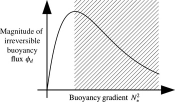
Central to Phillips’ argument is the flux-gradient relation due to the assumed inherent properties of stratified turbulence. The review by Linden (Reference Linden1979) of numerous experiments supported the existence of such a regime where flux decreases with gradient, i.e. the ‘right flank’ of Phillips’ curve (figure 1). Subsequently, various possible flux-gradient relations in the right-flank regime have been discussed, e.g. see figure 1 of Balmforth, Llewellyn-Smith & Young (Reference Balmforth, Llewellyn-Smith and Young1998). Recently, statistical mechanics arguments developed by Venaille, Gostiaux & Sommeria (Reference Venaille, Gostiaux and Sommeria2017), assuming infinite Reynolds and Péclet numbers, suggest that some appropriate measure of the overall mixing efficiency, characterising the fraction of the kinetic energy loss by the fluid that leads to an irreversible gain in the potential energy due to mixing, varies non-monotonically with the overall gradient Richardson number if the background buoyancy profile contains a layered structure, whereas such a mixing efficiency asymptotes to a constant value of approximately 0.25 if the background buoyancy gradient is uniform. This suggests that the mixing properties of a sharp density interface may vary significantly from that of a linearly varying density profile (e.g. Shih et al. Reference Shih, Koseff, Ivey and Ferziger2005). In this paper, we investigate the following four specific questions about the mixing properties of a density interface subject to imposed vertical shear.
A schematic representation of the functional dependence of the irreversible buoyancy flux
 $\unicode[STIX]{x1D719}_{d}$
in terms of the buoyancy gradient
 $N_{\ast }^{2}$
, i.e. Phillip’s flux-gradient curve. The definitions of
 $\unicode[STIX]{x1D719}_{d}$
and
 $N_{\ast }^{2}$
are discussed further in § 3. The shaded portion corresponds to the regime in which the flux decreases with the gradient, i.e. the ‘right flank’ of the curve, and the unshaded portion corresponds to the ‘left flank’. The asymptotic properties at sufficiently high buoyancy gradient are deliberately left open.

-
(i) Does the diapycnal flux (or its ‘turbulent’ component) completely vanish when the stratification is particularly strong, or does the mixing efficiency saturate to a constant as in standard turbulence parameterisations (e.g. Mellor & Yamada Reference Mellor and Yamada1982), and as apparently observed in vertically stratified Taylor–Couette flow between two concentric cylinders by Oglethorpe, Caulfield & Woods (Reference Oglethorpe, Caulfield and Woods2013)?
-
(ii) Does the molecular diffusivity of the fluid affect the overall mixing properties of the system? In particular, how does the mixing efficiency in the layered system compare to recent numerical results obtained in other flow configurations, e.g. those studied by Maffioli, Brethouwer & Lindborg (Reference Maffioli, Brethouwer and Lindborg2016) and Salehipour et al. (Reference Salehipour, Peltier, Whalen and MacKinnon2016b )?
-
(iii) Does there exist a self-sustaining mechanism which can act to keep the interface sharp and maintain the layered structure?
-
(iv) If so, what are the ingredients of the mechanism, and is it possible to relate the self-sharpening process to vertical variations in the mixing properties, analogously to Phillips’ argument?
It is well known that interfacial internal waves are important dynamical features associated with strongly stratified density interfaces. These waves may contribute, along with other relatively large-scale stirring processes, to the reversible component of buoyancy flux, thus introducing ambiguity to inferences of mixing from the conventional definition of buoyancy flux, i.e. the correlation between density and vertical velocity fluctuations (see e.g. the detailed discussion by Venayagamoorthy & Koseff Reference Venayagamoorthy and Koseff2016). A rigorous framework concerning the potential energy balance in a control volume was developed by Winters et al. (Reference Winters, Lombard, Riley and D’Asaro1995) and employed for analysing the bulk properties (such as mixing efficiency) of mixing layers, e.g. by Caulfield & Peltier (Reference Caulfield and Peltier2000). A variant of the above formalism involves a tracer-based reference ‘vertical’ coordinate which was formulated by Nakamura (Reference Nakamura1996) and Winters & D’Asaro (Reference Winters and D’Asaro1996), which has been used, for example, to quantify mixing in idealised two-dimensional flows (Nakamura Reference Nakamura1996; Shuckburgh & Haynes Reference Shuckburgh and Haynes2003) and in large-scale geophysical situations (Marshall et al. Reference Marshall, Shuckburgh, Jones and Hill2006). In this paper, we use the formulation introduced by Nakamura (Reference Nakamura1996) and Winters & D’Asaro (Reference Winters and D’Asaro1996) to examine the structural details of fluxes and diffusivities as they vary in the tracer-based coordinate, here employed to describe three-dimensional DNS data. As will be shown, this approach provides a useful framework for analysing the irreversible mixing, as well as the sharpening or maintenance of a density interface.
The rest of the paper is structured as follows. In § 2 we describe the numerical simulations of the layered stratified plane Couette flows and present qualitative observations on the time evolution of an originally sharp density interface. In § 3 the formalism which involves a tracer-based reference coordinate is reviewed, and we propose a possible self-sharpening mechanism by examining the local budget of buoyancy gradient in such reference coordinates. In § 4 we focus on the dynamics of a highly stable density interface and discuss the proposed self-sharpening mechanism in the framework that is presented in § 3 using DNS data. In § 5 the dependence of effective diffusivity and overall mixing efficiency on the characteristic parameters of the flow is discussed. In § 6 we provide some concluding remarks.
2 Numerical simulations
2.1 Simulation set-up
DNS of layered stratified plane Couette (LSPC) flows are considered in this paper, and these simulations follow closely those of Deusebio, Caulfield & Taylor (Reference Deusebio, Caulfield and Taylor2015) and Zhou, Taylor & Caulfield (Reference Zhou, Taylor and Caulfield2017). A full description of the DNS algorithms is presented in Taylor (Reference Taylor2008). In these simulations, we consider the velocity vector
 $\boldsymbol{u}=(u,v,w)$
in the coordinate system
 $\boldsymbol{x}=(x,y,z)$
, where
 $x$
and
 $y$
are the periodic (horizontal) directions and
 $z$
the wall-normal (vertical) direction. The incompressible Navier–Stokes equations under the Boussinesq approximation, i.e.
 $$\begin{eqnarray}\displaystyle & \displaystyle \frac{\unicode[STIX]{x2202}\boldsymbol{u}}{\unicode[STIX]{x2202}t}+\boldsymbol{u}\boldsymbol{\cdot }\unicode[STIX]{x1D735}\boldsymbol{u}=-\frac{\unicode[STIX]{x1D735}p}{\unicode[STIX]{x1D70C}_{0}}+\unicode[STIX]{x1D708}\unicode[STIX]{x1D6FB}^{2}\boldsymbol{u}+b\boldsymbol{e}_{z}, & \displaystyle\end{eqnarray}$$
 $$\begin{eqnarray}\displaystyle & \displaystyle \frac{\unicode[STIX]{x2202}b}{\unicode[STIX]{x2202}t}+\boldsymbol{u}\boldsymbol{\cdot }\unicode[STIX]{x1D735}b=\unicode[STIX]{x1D705}\unicode[STIX]{x1D6FB}^{2}b, & \displaystyle\end{eqnarray}$$
 $$\begin{eqnarray}\displaystyle & \unicode[STIX]{x1D735}\boldsymbol{\cdot }\boldsymbol{u}=0, & \displaystyle\end{eqnarray}$$
 $\unicode[STIX]{x1D708}$
and
 $\unicode[STIX]{x1D705}$
are the kinematic viscosity and the scalar diffusivity respectively. The buoyancy
 $$\begin{eqnarray}b\equiv -\frac{\unicode[STIX]{x1D70C}}{\unicode[STIX]{x1D70C}_{0}}g\end{eqnarray}$$
is proportional to the gravity
 $g$
and the density deviation
 $\unicode[STIX]{x1D70C}(\boldsymbol{x},t)$
from the reference density
 $\unicode[STIX]{x1D70C}_{0}$
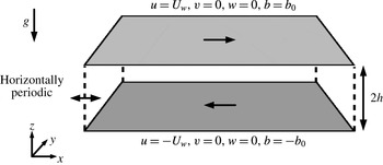
. Dirichlet boundary conditions for both velocity and buoyancy are applied at two horizontal non-slip walls as shown in figure 2. The walls move at the same speed
 $U_{w}$
in opposite directions in
 $x$
with a fixed buoyancy difference of
 $2b_{0}$
between them, i.e.
 $$\begin{eqnarray}(u,v,w,b)=(\pm U_{w},0,0,\pm b_{0})\quad \text{at}~z=\pm h\end{eqnarray}$$
respectively, resulting in a statically stable stratified shear flow system. Note that we use the ‘geophysical’ coordinate system, where
 $z$
is the wall-normal vertical direction in which gravity acts,
 $x$
is the streamwise direction with the flow driven by the relative motion of the walls and
 $y$
is the spanwise direction (see figure 2). Unless otherwise indicated in the remainder of the paper, velocities are normalised by
 $U_{w}$
, lengths are normalised by
 $h$
, buoyancy
 $b$
is normalised by
 $b_{0}$
and time
 $t$
is normalised by
 $h/U_{w}$
(i.e. the ‘advective’ time unit).
Three external parameters, i.e. the Reynolds number
 $\mathit{Re}$
, the (bulk) Richardson number
 $\mathit{Ri}$
and the Prandtl number
 $\mathit{Pr}$
, can be used to describe the flow. They are defined, respectively, as
 $$\begin{eqnarray}\mathit{Re}\equiv \frac{U_{w}h}{\unicode[STIX]{x1D708}},\quad \mathit{Ri}\equiv \frac{b_{0}h}{U_{w}^{2}}\quad \text{and}\quad \mathit{Pr}\equiv \frac{\unicode[STIX]{x1D708}}{\unicode[STIX]{x1D705}}.\end{eqnarray}$$
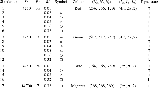
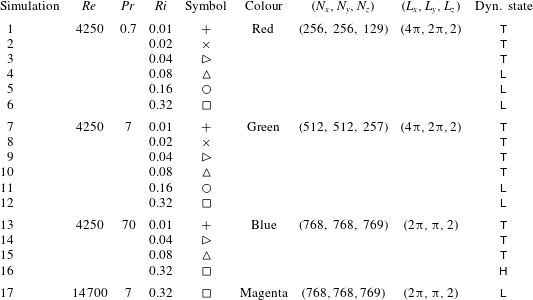
A total of 17 simulations are performed varying all three control parameters. The details of these simulations are summarised in table 1. Symbol types and colours (associated with each of the simulations) which are used in the subsequent figures are also shown in table 1. The choice of grid resolution in each simulation follows the specifications of Zhou et al. (Reference Zhou, Taylor and Caulfield2017) for fully developed turbulent stratified plane Couette flows. The values of
 $\mathit{Pr}$
considered in this paper include 0.7, 7 and 70. The first two values correspond to heat in air (
 $\mathit{Pr}=0.7$
) and heat in water (
 $\mathit{Pr}=7$
) respectively, and the largest value, i.e. 70, is included in an attempt to investigate the poorly diffusive regime corresponding to salt in water with a Schmidt number of approximately 700 (which is currently prohibitively costly to simulate with available resources).
Configuration of stratified plane Couette flow and boundary conditions.

2.2 Initial conditions
The simulations considered in this paper are designed to examine the time evolution of an initially sharp density interface subject to imposed vertical shear and buoyancy difference across the interface. We are specifically interested in how the interface interacts with pre-existing turbulent motions that are external to the interface, i.e. what we will later describe as the ‘scouring’ mechanism for mixing (see Woods et al.
Reference Woods, Caulfield, Landel and Kuesters2010). The initial conditions used in our simulations are, therefore, considerably different from typical initial value problems concerning stratified shear instabilities investigated by rundown simulations. The latter simulations are typically initialised by specific mean profiles of
 $u(z)$
and
 $b(z)$
within a ‘clean’ laminar background with turbulence generated only by the break down of the instability itself, as in e.g. computational studies of Kelvin–Helmholtz and Holmboe instabilities (Salehipour & Peltier Reference Salehipour and Peltier2015; Salehipour, Caulfield & Peltier Reference Salehipour, Caulfield and Peltier2016a
).
Summary of the numerical simulations of LSPC flows.
 $(N_{x},N_{y},N_{z})$
are the number of grid points used in each direction, and
 $(L_{x},L_{y},L_{z})$
are the lengths of computational domain. The last column lists the final dynamical state approached by each simulation:
 $\mathsf{T}$
for ‘turbulent’;
 $\mathsf{L}$
for ‘laminarising’; and
 $\mathsf{H}$
for ‘Holmboe’, all of which are described further in § 2.3.
The initial velocity field
 $\boldsymbol{u}(\boldsymbol{x},t=0)$
for our ‘production’ simulations is obtained by auxiliary simulations performed in two stages: first, unstratified plane Couette flow (
 $\mathit{Ri}=0$
) is simulated until it reaches a fully turbulent statistically stationary state. The purpose of this step is to produce a fully turbulent flow field spanning the channel gap. Second, in a ‘relaxation stage’ a sharp density interface with a hyperbolic tangent profile in
 $z$
 $$\begin{eqnarray}b(z)=b_{0}\tanh \left(\frac{z}{\unicode[STIX]{x1D6FF}_{0}}\right),\end{eqnarray}$$
where
 $\unicode[STIX]{x1D6FF}_{0}/h=0.08$
, is introduced. The value of
 $\unicode[STIX]{x1D6FF}_{0}/h$
controls the initial ‘sharpness’ of the interface, i.e. the thickness of the interface,
 $\unicode[STIX]{x1D6FF}_{0}$
, as compared to the half-channel gap length,
 $h$
, which characterises the length scale typical of large-scale energy-containing eddies in the turbulence between and wall and the density interface. Although it would be of interest to explore the dynamical effects of varying this ratio, for clarity we here only consider this one specific value, sufficiently small so that the interface is adequately ‘sharp’. All relaxation simulations are performed at
 $(\mathit{Ri},\mathit{Pr})=(0.08,0.7)$
and the Reynolds number is the same as in the unstratified simulation. The purpose of the relaxation stage is to reduce the excessive amount of turbulent kinetic energy (TKE) locally at the centre of the channel gap around the interface, so that the interface maintains its structural integrity at least at the beginning of the main ‘production’ simulations. This TKE reduction is achieved by resetting
 $\langle b\rangle (z)$
, i.e. the mean value of
 $b$
averaged over a horizontal plane, to the initial hyperbolic tangent profile (2.5) at the end of every time step in the simulation, while allowing the perturbations
 $b^{\prime }(\boldsymbol{x},t)=b(\boldsymbol{x},t)-\langle b\rangle (z)$
and velocity field
 $\boldsymbol{u}(\boldsymbol{x},t)$
to evolve in time. The strong stratification which is artificially maintained by resetting the mean buoyancy profile suppresses the turbulent motions in the vicinity of the interface and hence reduces the local values of TKE.
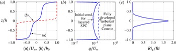
Vertical profiles of mean quantities corresponding to the initial condition used in the LSPC flow simulations with
 $\mathit{Re}=4250$
. (a) Mean velocity
 $\langle u\rangle$
(plotted with a solid line) and buoyancy
 $\langle b\rangle$
(plotted with a dashed line). (b) Initial condition for the turbulent velocity scale
 $q$
for a layered stratified plane Couette flow simulation (plotted with a solid line) and a fully turbulent unstratified (
 $\mathit{Ri}=0$
) plane Couette flow simulation at the same
 $\mathit{Re}$
(plotted with a dashed line). (c) Profile of initial gradient Richardson number
 $\mathit{Ri}_{g}(z,t=0)$
, based on horizontal averages as defined in (2.7), divided by the bulk Richardson number
 $Ri$
.

The volume-integrated TKE value reaches a minimum after running the relaxation procedure for
 $t\approx 60h/U_{w}$
, and the velocity field
 $\boldsymbol{u}(\boldsymbol{x})$
at this minimum TKE state is used to initialise the production simulations. A ‘fresh’ density field
 $b(z)$
following (2.5) is also introduced at the beginning of the production simulations, when the values of
 $\mathit{Pr}$
and
 $\mathit{Ri}$
are reset to those defined in table 1 of a particular simulation. Three sets of initial
 $\boldsymbol{u}$
fields are obtained using the same procedure (but varying
 $\mathit{Re}$
or domain size), each applied to simulations 1–12, 13–16 and 17, i.e. for simulations within each of the three groups, the initial
 $\boldsymbol{u}$
fields are identical.
Figure 3 shows typical vertical profiles describing the initial conditions of the simulations. The sharp buoyancy interface located at
 $z=0$
is embedded within a sheared velocity profile. The mean vertical shear is stronger both at the centre of the channel gap where the density interface is located and in the viscous wall regions. As previously discussed, the initial
 $\boldsymbol{u}$
field is turbulent with the profile (as shown in figure 3
b) of the turbulent velocity scale
 $q(z,t)$
defined as
 $$\begin{eqnarray}q(z,t)\equiv \sqrt{\langle u^{\prime 2}+v^{\prime 2}+w^{\prime 2}\rangle },\end{eqnarray}$$
where
 $\langle \cdot \rangle$
indicates a spatial horizontal average over an
 $x$
–
 $y$
plane and
 $(u^{\prime },v^{\prime },w^{\prime })$
denote fluctuation velocities from the horizontal mean. The magnitude of
 $q$
in the channel interior is approximately 10 % of the wall speed
 $U_{w}$
and is reduced by approximately 40 % from the unstratified fully turbulent plane Couette flow at the same
 $\mathit{Re}$
. Again, this particular initial condition of
 $\boldsymbol{u}$
is designed specifically to prevent the interface from being broken up by strong turbulent motions when the interface is introduced at
 $t=0$
. The mean gradient Richardson number,
 $$\begin{eqnarray}\mathit{Ri}_{g}(z,t)\equiv \frac{N^{2}}{S^{2}}=\frac{\unicode[STIX]{x2202}\langle b\rangle /\unicode[STIX]{x2202}z}{(\unicode[STIX]{x2202}\langle u\rangle /\unicode[STIX]{x2202}z)^{2}},\end{eqnarray}$$
which is based on horizontal averages denoted by
 $\langle \cdot \rangle$
, is plotted in figure 3(c) for
 $t=0$
. As expected, the
 $\mathit{Ri}_{g}$
value peaks at the density interface centred at
 $z=0$
and is virtually zero within the uniform density layers above and below the interface, i.e.
 $|z/h|\gtrsim 0.4$
.
2.3 Qualitative observations
Once initialised at
 $t=0$
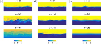
, the stratified interface is subject to the mean and turbulent motions maintained by the forcing of the walls. For flows with different external parameters, the interface exhibits different behaviours and approaches three possible dynamical states as tabulated in table 1. The three possible states shown in figure 4 are:
Side view of typical buoyancy field
 $b(x,y=0,z)$
at various times for (a) simulation 10:
 $(\mathit{Pr},\mathit{Ri})=(7,0.08)$
, corresponding to
 $\mathsf{T}$
state, (b) simulation 16:
 $(\mathit{Pr},\mathit{Ri})=(70,0.32)$
, corresponding to
 $\mathsf{H}$
state, and (c) simulation 12:
 $(\mathit{Pr},\mathit{Ri})=(7,0.32)$
, corresponding to
 $\mathsf{L}$
state. The visualisation window is
 $2\unicode[STIX]{x03C0}h$
long in
 $x$
(corresponding to half of the domain length,
 $0.5L_{x}$
, for simulations 10 and 12, and the full domain length,
 $L_{x}$
, for simulation 16) and
 $2h$
tall in
 $z$
.

(i) The ‘turbulent’ state
 $\mathsf{T}$
as shown in figure 4(a) for simulation 10. For relatively weakly stratified flows with
 $\mathit{Ri}\leqslant 0.04$
for
 $\mathit{Pr}=0.7$
or
 $\mathit{Ri}\leqslant 0.08$
for
 $\mathit{Pr}=7$
and 70 (see table 1), the stratification is too weak to suppress the turbulence. The interface soon becomes highly disordered with spatially intermittent shear-induced local overturns where vigorous mixing occurs. As a result, the sharpness of the interface is not robust, with the thickness of the interface increasing with time and the system approaching a fully turbulent, stratified, yet definitely not layered state.
(ii) The ‘Holmboe’ state
 $\mathsf{H}$
is shown in figure 4(b) where the interface stays robust. The
 $\mathsf{H}$
state is observed in simulation 16 with large values of both
 $\mathit{Ri}$
and
 $\mathit{Pr}$
, i.e.
 $\mathit{Ri}=0.32$
and
 $\mathit{Pr}=70$
. Structures strongly reminiscent of ‘Holmboe waves’ (see e.g. figure 4 of Smyth, Klaassen & Peltier (Reference Smyth, Klaassen and Peltier1988) and figure 4 of Salehipour et al. (Reference Salehipour, Caulfield and Peltier2016a
)) appear to develop on the interface, and these structures prove to be long lived and robust. ‘Cusp’ structures at the crests of the wave, along with concentrated spanwise vorticity, i.e.
 $\unicode[STIX]{x1D714}_{y}$
, appear on both sides of the interface associated with these Holmboe-wave-like structures. As is typical, the cusps above and below the interface are observed to propagate in opposite directions. The vortices on either side of the interface act to entrain fluid from the interface, contributing to the ‘wisps’ structure in the lee of the ‘cusps’ in their direction of propagation, similar to the simulations of Smyth et al. (Reference Smyth, Klaassen and Peltier1988) and Salehipour et al. (Reference Salehipour, Caulfield and Peltier2016a
). It is important to note that all the propagating disturbances observed on the interface have characteristic phase speeds in the range
 $-U_{w}<c_{ph}<U_{w}$
, and so none of the wave-like motions observed on the interface should be interpreted as ‘pure’ interfacial internal waves, unrelated to flow instabilities (specifically the Holmboe wave instability). The interface is observed to stay sharp, and the dynamics is dominated by internal waves rather than shear-induced turbulent overturns. The dynamics of the
 $\mathsf{H}$
state is also strongly reminiscent of the experimental observations of Holmboe waves on a sheared density interface by Strang & Fernando (Reference Strang and Fernando2001), who also reported buoyancy fluxes and entrainment rates based on planar laser-induced fluorescence measurements. The three-dimensional velocity and buoyancy fields obtained from direct numerical simulations allow us to consider the irreversible diapycnal mixing processes in detail, as is presented in the remainder of this paper.
(iii) The ‘laminarising’ state
 $\mathsf{L}$
is shown in figure 4(c) for simulation 12. This
 $\mathsf{L}$
state exists at large
 $\mathit{Ri}$
values for which stratification is able to suppress turbulence. Simulation 12, shown as an example of the
 $\mathsf{L}$
state, has the same
 $\mathit{Re}$
and
 $\mathit{Ri}$
values as simulation 16, shown for the
 $\mathsf{H}$
state, but the
 $\mathit{Pr}$
value is 7 instead of 70. Internal waves similar to those in the
 $\mathsf{H}$
state appear at early times of the
 $\mathsf{L}$
state. The amplitude of the wave motion, however, noticeably decays with time, while the thickness of the interface gradually increases, presumably due to molecular diffusion. The flow is observed to approach the laminar steady state solution with
 $u/U_{w}=b/b_{0}=z/h$
(Eliassen, Hailand & Riis Reference Eliassen, Hailand and Riis1953).
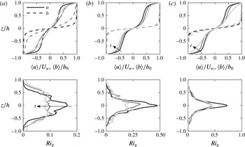
As an aside, we can investigate the linear stability properties of the flows described above by examining the horizontally averaged, instantaneous velocity and buoyancy profiles shown in figure 5. Simulations presented in figure 5 and the times at which the mean profiles are sampled are identical to those shown in figure 4. In order to examine the linear stability of these mean profiles, the viscous, diffusive and stratified eigenvalue problem, e.g. as described in (3.6) and (3.7) of Eaves & Caulfield (Reference Eaves and Caulfield2017), is solved numerically using the procedure described in Smyth, Moum & Nash (Reference Smyth, Moum and Nash2011). Mean profiles associated with the
 $\mathsf{T}$
-state simulation 10 are shown in figure 5(a). While the gradient Richardson number,
 $\mathit{Ri}_{g}$
associated with these averaged profiles is smaller than 0.2 (shown in the lower panel), the mean profiles are found to be linearly stable. However, the flow stays turbulent (see figure 4
a) as it evolves from the already turbulent initial condition (see figure 3
b) to reaching the fully developed turbulent state (see e.g. Zhou et al.
Reference Zhou, Taylor and Caulfield2017).
For the
 $\mathsf{H}$
-state simulation 16 shown in figure 5(b) and the
 $\mathsf{L}$
-state simulation 12 shown in figure 5(c), the mean profiles analysed are all unstable to instabilities which can be identified as being of Holmboe type. This identification can be made for several reasons. The
 $\mathit{Ri}_{g}$
distribution has the peaked structure associated with Holmboe-type instabilities. Furthermore, the velocity structure has strong shear over a relatively sharp interface, dropping to weaker shear either side. Such a structure is entirely characteristic of Holmboe-type instabilities, which can be interpreted as arising due to the interaction of an internal wave localised at the density interface, and a Doppler-shifted vorticity or ‘Rayleigh’ wave localised at the edge of the shear layer (Caulfield Reference Caulfield1994; Baines & Mitsudera Reference Baines and Mitsudera1994; Carpenter et al.
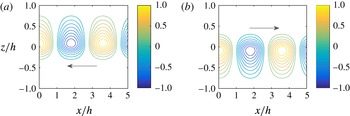
Reference Carpenter, Tedford, Heifetz and Lawrence2011). Finally, the eigenfunction corresponding to the fastest growing Holmboe-type mode is plotted in figure 6, showing the characteristic structure centred above and below the ‘sharp’ density interface, leading to the characteristic propagation of the disturbance relative to the density interface (see Carpenter, Balmforth & Lawrence (Reference Carpenter, Balmforth and Lawrence2010) for further discussion of instability classification in stratified shear flows).
Horizontally averaged velocity, buoyancy and gradient Richardson number profiles for: (a) simulation 10 at
 $(\mathit{Pr},\mathit{Ri})=(7,0.08)$
(
 $\mathsf{T}$
state); (b) simulation 16 at
 $(\mathit{Pr},\mathit{Ri})=(70,0.32)$
(
 $\mathsf{H}$
state); and (c) simulation 12 at
 $(\mathit{Pr},\mathit{Ri})=(7,0.32)$
(
 $\mathsf{L}$
state). The profiles are sampled at the same times at which the buoyancy field is shown in figure 4 with lighter line shades corresponding to later times in each simulation.

Typical structure of the vertical velocity eigenfunctions associated with the fastest growing modes of linear theory corresponding to Holmboe-type instabilities. The eigenfunctions are obtained for the mean profiles shown in figure 5(b) at
 $t=84$
(darkest line) for simulation 16 (
 $\mathsf{H}$
state). The eigenfunctions shown in both panels, (a) and (b), have the same growth rate
 $\unicode[STIX]{x1D70E}\simeq 0.00171$
and equal and opposite real phase velocity
 $c_{ph}\simeq \mp 0.338$
(the arrow in each panel indicates the direction of
 $c_{ph}$
). The streamwise velocity component has higher magnitude, peaked on the other side of the
 $z$
-midplane for these eigenfunctions, and so the perturbation kinetic energy of both these modes is peaked (as expected) in the vicinity of the location where the phase velocity of the perturbation coincides with the velocity of the background flow. The streamwise wavenumber associated with these fastest growing modes is
 $k_{x}\simeq 1.75$
.

It also is important to note that the profiles at
 $t\,=\,348$
for simulation 16 (
 $\mathsf{H}$
state) are unstable also to Kelvin–Helmholtz-type instabilities, centred on the density interface. However, the Holmboe-wave-like structures only survive in the
 $\mathsf{H}$
state, but not in the
 $\mathsf{L}$
state, even though the linear analysis predicts the mean profiles are unstable to Holmboe instability in both cases. This analysis suggests that linear stability analysis based on the mean profiles should be used with caution when predicting the evolution of these density interfaces, at least when the underlying base flows are initially turbulent and the mean profiles vary significantly in time. This is not entirely surprising, because the substantial temporal and spatial variations of the actual streamwise velocity and buoyancy profiles about the horizontally averaged mean profiles preclude infinitesimal perturbations experiencing for any extended period of time the notional profiles in which those infinitesimal perturbations are predicted to be (linearly) unstable.
As discussed above, our goal is to describe the behaviour of a pre-existing density interface subject to vertical shear from the perspective of diapycnal mixing. We are particularly interested in any self-sustaining (and hence inherently nonlinear) mechanism which keeps the interface sharp, and the existence of the
 $\mathsf{H}$
state described above provides a dataset which can be analysed to identify and describe such mechanisms. In the following section (§ 3), the mathematical formalism we employ to describe the diapycnal mixing is described, and in § 4 we focus on investigating the
 $\mathsf{H}$
state by comparing it to the
 $\mathsf{L}$
state as both
 $\mathsf{L}$
and
 $\mathsf{H}$
states can occur in large-
 $\mathit{Ri}$
strongly stratified systems. All
 $\mathsf{T}$
,
 $\mathsf{H}$
and
 $\mathsf{L}$
states are included in the considerations of mixing properties discussed in § 5.
3 Mathematical formulation
3.1 Tracer-based coordinate, flux and diffusivity
The formalism developed by Nakamura (Reference Nakamura1996) and Winters & D’Asaro (Reference Winters and D’Asaro1996) is used to quantify the diapycnal mixing of the stratifying agent, i.e. the dynamic scalar tracer within the flow. This framework considers the mixing of a conserved tracer in a ‘sorted’ reference coordinate
 $z_{\ast }$
. The definition of this
 $z_{\ast }$
coordinate relates to the ‘background’ buoyancy profile which is obtained by sorting all fluid parcels adiabatically to reach the minimum possible potential energy of the system, i.e. the background potential energy (see e.g. Winters et al.
Reference Winters, Lombard, Riley and D’Asaro1995). In the present study, we approximate the background buoyancy profile (or the ‘sorted’ profile)
 $b(z_{\ast },t)$
via the probability density function (p.d.f.) method introduced by Tseng & Ferziger (Reference Tseng and Ferziger2001) which avoids the explicit sorting procedure but is formally equivalent in the limit as the ‘bins’ used in constructing the p.d.f. become arbitrarily small.
Following the Winters–D’Asaro–Nakamura formalism, the diapycnal flux
 $\unicode[STIX]{x1D719}_{d}$
across a specific isopycnal (constant buoyancy
 $b$
) surface corresponding to a particular reference position
 $z_{\ast }$
can be defined by a simple flux-gradient relation
 $$\begin{eqnarray}\unicode[STIX]{x1D719}_{d}\equiv -\unicode[STIX]{x1D705}_{e}\frac{\unicode[STIX]{x2202}b}{\unicode[STIX]{x2202}z_{\ast }},\end{eqnarray}$$
where
 $\unicode[STIX]{x1D705}_{e}(z_{\ast },t)$
is an effective diapycnal diffusivity and the gradient
 $\unicode[STIX]{x2202}b/\unicode[STIX]{x2202}z_{\ast }$
can be obtained from the background buoyancy profile
 $b(z_{\ast },t)$
. The flux
 $\unicode[STIX]{x1D719}_{d}$
can be determined exactly from the instantaneous (dynamic) scalar field
 $b(\boldsymbol{x},t)$
via the following relation
 $$\begin{eqnarray}\unicode[STIX]{x1D719}_{d}=-\unicode[STIX]{x1D705}\frac{\unicode[STIX]{x2202}z_{\ast }}{\unicode[STIX]{x2202}b}\langle |\unicode[STIX]{x1D735}b|^{2}\rangle _{z_{\ast }},\end{eqnarray}$$
where
 $\langle \cdot \rangle _{z_{\ast }}$
indicates averaging over the isoscalar surface corresponding to the reference position
 $z_{\ast }$
, and
 $|\unicode[STIX]{x1D735}b|^{2}$
is given by the gradients of
 $b$
in the physical space
 $\boldsymbol{x}$
. By definition,
 $b$
increases monotonically with
 $z_{\ast }$
, i.e.
 $\unicode[STIX]{x2202}z_{\ast }/\unicode[STIX]{x2202}b>0$
, and the flux
 $\unicode[STIX]{x1D719}_{d}$
is negative definite (down gradient). It follows from (3.1) and (3.2) that the effective diffusivity
 $\unicode[STIX]{x1D705}_{e}$
can be estimated by
 $$\begin{eqnarray}\unicode[STIX]{x1D705}_{e}=\unicode[STIX]{x1D705}\left(\frac{\unicode[STIX]{x2202}z_{\ast }}{\unicode[STIX]{x2202}b}\right)^{2}\langle |\unicode[STIX]{x1D735}b|^{2}\rangle _{z_{\ast }},\end{eqnarray}$$
which yields a positive-definite value of
 $\unicode[STIX]{x1D705}_{e}$
. The geometrical interpretation of (3.3) is given by equation (12) of Winters & D’Asaro (Reference Winters and D’Asaro1996), i.e.
 $$\begin{eqnarray}\unicode[STIX]{x1D705}_{e}=\unicode[STIX]{x1D705}\left(\frac{A_{s}}{A}\right)^{2}\geqslant \unicode[STIX]{x1D705},\end{eqnarray}$$
where
 $A_{s}$
is the area of the isopycnal surface corresponding to buoyancy
 $b$
at a given reference position
 $z_{\ast }$
. A given value of
 $z_{\ast }$
corresponds to a set of points in the physical
 $\boldsymbol{x}=(x,y,z)$
coordinates. This set of points in
 $\boldsymbol{x}$
form the isopycnal surface(s) corresponding to the buoyancy value at the reference position
 $z_{\ast }$
in the sorted profile, i.e.
 $b(z_{\ast })$
. It is important to appreciate that the isopycnal surface(s) may have a distorted shape which may not be simply connected.
 $A$
in (3.4) is the area of the isopycnal surface projected onto a flat horizontal plane, i.e. the area of the flat undistorted surface. The increase of
 $A_{s}$
above
 $A$
is due to the straining imposed by the flow on the scalar field, and the effective diffusivity
 $\unicode[STIX]{x1D705}_{e}$
can thus be greatly enhanced from the molecular value
 $\unicode[STIX]{x1D705}$
due to the factor
 $(A_{s}/A)^{2}$
.
3.2 Evolution of background buoyancy profile
Nakamura (Reference Nakamura1996) and Winters & D’Asaro (Reference Winters and D’Asaro1996) showed that the advection–diffusion equation of any conserved tracer in an incompressible flow can be written exactly as a one-dimensional diffusion equation in the reference
 $z_{\ast }$
coordinate:
 $$\begin{eqnarray}\frac{\unicode[STIX]{x2202}b}{\unicode[STIX]{x2202}t}=-\frac{\unicode[STIX]{x2202}\unicode[STIX]{x1D719}_{d}}{\unicode[STIX]{x2202}z_{\ast }}=\frac{\unicode[STIX]{x2202}}{\unicode[STIX]{x2202}z_{\ast }}\left(\unicode[STIX]{x1D705}_{e}\frac{\unicode[STIX]{x2202}b}{\unicode[STIX]{x2202}z_{\ast }}\right).\end{eqnarray}$$
Taking the derivative of (3.5) with respect to
 $z_{\ast }$
yields an evolution equation for the buoyancy gradient in the reference coordinate
 $N_{\ast }^{2}\equiv \unicode[STIX]{x2202}b/\unicode[STIX]{x2202}z_{\ast }$
:
 $$\begin{eqnarray}\frac{\unicode[STIX]{x2202}N_{\ast }^{2}}{\unicode[STIX]{x2202}t}=\underbrace{\frac{\unicode[STIX]{x2202}^{2}\unicode[STIX]{x1D705}_{e}}{\unicode[STIX]{x2202}z_{\ast }^{2}}N_{\ast }^{2}}_{\text{Source}~\mathbb{S}(t)}+\underbrace{2\frac{\unicode[STIX]{x2202}\unicode[STIX]{x1D705}_{e}}{\unicode[STIX]{x2202}z_{\ast }}\frac{\unicode[STIX]{x2202}N_{\ast }^{2}}{\unicode[STIX]{x2202}z_{\ast }}}_{\text{Advection}~\mathbb{A}(t)}+\underbrace{\unicode[STIX]{x1D705}_{e}\frac{\unicode[STIX]{x2202}^{2}N_{\ast }^{2}}{\unicode[STIX]{x2202}z_{\ast }^{2}}}_{\text{Diffusion}~\mathbb{D}(t)}.\end{eqnarray}$$
The first bracketed term
 $\mathbb{S}(t)$
on the right-hand side of (3.6) corresponds to a source/sink term for
 $N_{\ast }^{2}$
depending on the sign of the prefactor
 $\unicode[STIX]{x2202}^{2}\unicode[STIX]{x1D705}_{e}/\unicode[STIX]{x2202}z_{\ast }^{2}$
, the curvature of
 $\unicode[STIX]{x1D705}_{e}$
. The second bracketed term
 $\mathbb{A}(t)$
corresponds to the advection of
 $N_{\ast }^{2}$
with a ‘velocity’ of
 $-2\unicode[STIX]{x2202}\unicode[STIX]{x1D705}_{e}/\unicode[STIX]{x2202}z_{\ast }$
. The third bracketed term
 $\mathbb{D}(t)$
corresponds to the diffusion of
 $N_{\ast }^{2}$
with the effective diffusivity
 $\unicode[STIX]{x1D705}_{e}$
in the
 $z_{\ast }$
coordinate. Note that (3.6) can alternatively be written as
 $$\begin{eqnarray}\frac{\unicode[STIX]{x2202}N_{\ast }^{2}}{\unicode[STIX]{x2202}t}=\frac{\unicode[STIX]{x2202}^{2}\unicode[STIX]{x1D705}_{e}}{\unicode[STIX]{x2202}z_{\ast }^{2}}N_{\ast }^{2}+\frac{\unicode[STIX]{x2202}\unicode[STIX]{x1D705}_{e}}{\unicode[STIX]{x2202}z_{\ast }}\frac{\unicode[STIX]{x2202}N_{\ast }^{2}}{\unicode[STIX]{x2202}z_{\ast }}+\frac{\unicode[STIX]{x2202}}{\unicode[STIX]{x2202}z_{\ast }}\left(\unicode[STIX]{x1D705}_{e}\frac{\unicode[STIX]{x2202}N_{\ast }^{2}}{\unicode[STIX]{x2202}z_{\ast }}\right),\end{eqnarray}$$
where the third term on the right-hand side corresponds to the divergence of the diffusive flux
 $\unicode[STIX]{x1D705}_{e}\unicode[STIX]{x2202}N_{\ast }^{2}/\unicode[STIX]{x2202}z_{\ast }$
in
 $z_{\ast }$
, but we adopt the subdivision of terms in (3.6) for the rest of the paper. As will be shown in the following section (§ 4), the diagnostic framework described here yields a robust description of the dynamics of temporally evolving density interfaces.
4 Dynamics of highly stable interfaces
4.1 Structure of diapycnal flux and effective diffusivity
In this section, we focus on simulations with
 $\mathit{Ri}=0.32$
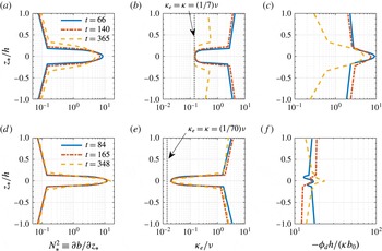
, the largest bulk Richardson number which we have considered, and investigate the dynamics of interfaces with such strong stratification that they are stable to shear-induced overturns. Figure 7 shows the profiles of effective diffusivity
 $\unicode[STIX]{x1D705}_{e}$
and diapycnal flux
 $\unicode[STIX]{x1D719}_{d}$
in the
 $z_{\ast }$
coordinate. Several times are shown for simulation 12 (
 $\mathsf{L}$
state) at
 $(\mathit{Pr},\mathit{Ri},\mathit{Re})=(7,0.32,4250)$
and for simulation 16 (
 $\mathsf{H}$
state) at
 $(\mathit{Pr},\mathit{Ri},\mathit{Re})=(70,0.32,4250)$
. Times associated with the profiles also correspond to the flow snapshots shown in (c) and (b) of figure 4 respectively.
Profiles of: background buoyancy gradient
 $N_{\ast }^{2}$
(a,d); effective diffusivity
 $\unicode[STIX]{x1D705}_{e}$
normalised by molecular kinematic viscosity
 $\unicode[STIX]{x1D708}$
(b,e); and magnitude of diapycnal flux
 $\unicode[STIX]{x1D719}_{d}$
normalised by
 $\unicode[STIX]{x1D705}b_{0}/h$
(c,f). (a–c) Correspond to simulation 12 with
 $\mathsf{L}$
state at
 $(\mathit{Pr},\mathit{Ri})=(7,0.32)$
, and (d–f) correspond to simulation 16 with
 $\mathsf{H}$
state at
 $(\mathit{Pr},\mathit{Ri})=(70,0.32)$
. Both simulations are at
 $\mathit{Re}=4250$
. Dotted vertical lines in (b,e) correspond to the minimum possible value of
 $\unicode[STIX]{x1D705}_{e}=\unicode[STIX]{x1D705}$
, or equivalently,
 $\unicode[STIX]{x1D705}_{e}/\unicode[STIX]{x1D708}=1/\mathit{Pr}$
. Profiles at various times are shown, and flow snapshots at these times can be found in figure 4. Note that the horizontal axes are shown on different scales in the two panels in (c,f) showing the
 $-\unicode[STIX]{x1D719}_{d}$
profiles.

As shown in figure 7(a), the buoyancy gradient
 $N_{\ast }^{2}$
at the midplane of the interface at
 $z_{\ast }=0$
decreases with time, and the thickness of the interface grows. The effective diffusivity
 $\unicode[STIX]{x1D705}_{e}$
takes the molecular value
 $\unicode[STIX]{x1D705}$
within the density interface located near
 $z_{\ast }=0$
, and as the interface grows thicker,
 $\unicode[STIX]{x1D705}_{e}$
approaches
 $\unicode[STIX]{x1D705}$
over a broader range of
 $z_{\ast }$
. This broadening suggests that the isopycnal surfaces are flattening, i.e.
 $A_{s}\rightarrow A$
as in (3.4), and the system is laminarising. The diapycnal flux
 $\unicode[STIX]{x1D719}_{d}$
varies significantly in
 $z_{\ast }$
, and the divergence of the flux drives the broadening of the interface.
As is shown in figure 7(b), by varying
 $\mathit{Pr}$
alone from
 $7$
to
 $70$
, simulation 16 is in the
 $\mathsf{H}$
state rather than the
 $\mathsf{L}$
state. The gradient
 $N_{\ast }^{2}$
at the midplane is observed to increase (though weakly) with time and the interface thickness remains approximately unchanged, which is consistent with the observations in figure 4(b) that the interface is robust and long lived. The ratio
 $\unicode[STIX]{x1D705}_{e}/\unicode[STIX]{x1D708}$
now takes smaller values at the midplane as the lower bound determined by molecular diffusivity
 $\min (\unicode[STIX]{x1D705}_{e}/\unicode[STIX]{x1D708})=\unicode[STIX]{x1D705}/\unicode[STIX]{x1D708}=1/\mathit{Pr}$
is smaller due to the larger
 $\mathit{Pr}$
, which allows for a wide range of
 $\unicode[STIX]{x1D705}_{e}/\unicode[STIX]{x1D708}$
from slightly above
 $1/\mathit{Pr}\sim O(0.01)$
around the midplane to
 $O(1)$
away from the interface at
 $z_{\ast }/h\approx \pm 0.1$
. The flux
 $\unicode[STIX]{x1D719}_{d}$
is close to constant with
 $z_{\ast }$
, and in the absence of a significant divergence of the flux, the strong gradient at the interface is expected to stay constant in time and last indefinitely.
The profiles shown in figure 7 also allow us to consider the role of various terms on the right-hand side of (3.6) which govern the time evolution of the buoyancy gradient
 $N_{\ast }^{2}$
. In both simulations considered in figure 7, the source term
 $\mathbb{S}(t)$
is positive and acts to sharpen the local gradient, but the prefactor corresponding to the curvature of
 $\unicode[STIX]{x1D705}_{e}$
, i.e.
 $\unicode[STIX]{x2202}^{2}\unicode[STIX]{x1D705}_{e}/\unicode[STIX]{x2202}z_{\ast }^{2}$
, is significantly larger for the
 $\mathsf{H}$
state. The advection term
 $\mathbb{A}(t)$
is expected to be non-positive as
 $\unicode[STIX]{x2202}\unicode[STIX]{x1D705}_{e}/\unicode[STIX]{x2202}z_{\ast }$
and
 $\unicode[STIX]{x2202}N_{\ast }^{2}/\unicode[STIX]{x2202}z_{\ast }$
tend to take opposite signs for a given
 $z_{\ast }$
, but at the midplane of the interface
 $\mathbb{A}(t)$
is expected to be zero as
 $\unicode[STIX]{x2202}\unicode[STIX]{x1D705}_{e}/\unicode[STIX]{x2202}z_{\ast }=\unicode[STIX]{x2202}N_{\ast }^{2}/\unicode[STIX]{x2202}z_{\ast }=0$
at
 $z_{\ast }=0$
due to the symmetry of the profiles about the midplane. The diffusion term
 $\mathbb{D}(t)$
is expected to weaken the gradient within the interface as
 $\unicode[STIX]{x1D705}_{e}$
is positive definite. Therefore, in order for an interface to be maintained, the source term
 $\mathbb{S}(t)$
must be able to counterbalance the effects of the other two terms. We investigate this balance quantitatively in § 4.2.
The sign of
 $\unicode[STIX]{x2202}^{2}\unicode[STIX]{x1D705}_{e}/\unicode[STIX]{x2202}z_{\ast }^{2}$
serves as a simple diagnostic quantity to examine if any sharpening process is present around a density interface. Turbulence and/or vortical structures induced by Holmboe waves, which are displaced from the interface, could conceivably act on either side of the interface to ‘scour’ the material away from the interface via the ‘wisps’ structures that are clearly visible in figure 4(b). (Such a behaviour appears at least qualitatively to be occurring in the rundown simulations susceptible to Holmboe wave instabilities described in Salehipour et al.
Reference Salehipour, Caulfield and Peltier2016a
.) In this case, an isopycnal surface away from the midplane
 $z_{\ast }=0$
would have a more convoluted shape and thus larger surface area
 $A_{s}$
and hence larger
 $\unicode[STIX]{x1D705}_{e}$
following (3.4). On the other hand, in the middle of the interface the flow exhibits minimal wave disturbances or turbulence, and the isopycnal surface is nearly flat with
 $A_{s}\approx A$
. Thus
 $\unicode[STIX]{x1D705}_{e}$
is expected to increase away from the midplane of the interface, consistent with the observations in figure 7. It is then possible to have a positive curvature of the
 $\unicode[STIX]{x1D705}_{e}(z_{\ast })$
profile, i.e.
 $\unicode[STIX]{x2202}^{2}\unicode[STIX]{x1D705}_{e}/\unicode[STIX]{x2202}z_{\ast }^{2}>0$
, in the presence of mixing associated with scouring. When the scouring effect is large enough to overcome diffusion, i.e.
 $|\mathbb{S}(t)|>|\mathbb{D}(t)|$
, the flow may act to enhance the local gradient
 $N_{\ast }^{2}$
. The reverse is true when one considers mixing due to large overturns, e.g. due to Kelvin–Helmholtz instability (KHI). The isopycnal surface in the overturning case is expected to have the most convoluted surface with large
 $A_{s}/A$
ratio in the core region of the KHI finite amplitude ‘billow’ where the maximum
 $\unicode[STIX]{x1D705}_{e}$
is attained. The magnitude of
 $\unicode[STIX]{x1D705}_{e}$
decreases with the distance to the midplane
 $z_{\ast }=0$
, which may lead to
 $\unicode[STIX]{x2202}^{2}\unicode[STIX]{x1D705}_{e}/\unicode[STIX]{x2202}z_{\ast }^{2}<0$
and thus negative values of
 $\mathbb{S}(t)$
. The
 $\mathbb{S}(t)$
term then reduces the local
 $N_{\ast }^{2}$
value in concert with the diffusion term
 $\mathbb{D}(t)$
, both acting to destroy the density interface through overturning dynamics.
4.2 Time evolution of the buoyancy gradient with respect to
 $z_{\ast }$

In this subsection, we further examine the time evolution of various budget terms in (3.6) for the local gradient
 $N_{\ast }^{2}$
. First, the integral thickness
 $\unicode[STIX]{x1D6FF}_{\ast }$
of the density interface can be calculated from the sorted buoyancy profile by
 $$\begin{eqnarray}\unicode[STIX]{x1D6FF}_{\ast }\equiv \frac{1}{2b_{0}}\left[\int _{-h}^{0}(b_{0}+b)\,\text{d}z_{\ast }+\int _{0}^{h}(b_{0}-b)\,\text{d}z_{\ast }\right],\end{eqnarray}$$
where
 $b_{0}=b(z_{\ast }=h)=-b(z_{\ast }=-h)$
, and the buoyancy difference across the interface
 $\unicode[STIX]{x0394}b$
can be calculated as
 $$\begin{eqnarray}\unicode[STIX]{x0394}b\equiv {\textstyle \frac{1}{2}}[b(z_{\ast }=\unicode[STIX]{x1D6FF}_{\ast })-b(z_{\ast }=-\unicode[STIX]{x1D6FF}_{\ast })].\end{eqnarray}$$
The volume (depth) averaged value of an arbitrary quantity
 ${\mathcal{F}}(z_{\ast },t)$
over the density interface
 $-\unicode[STIX]{x1D6FF}_{\ast }<z_{\ast }<\unicode[STIX]{x1D6FF}_{\ast }$
is denoted with an overbar, and defined as
 $$\begin{eqnarray}\overline{{\mathcal{F}}}(t)\equiv \frac{\displaystyle \int _{-\unicode[STIX]{x1D6FF}_{\ast }}^{\unicode[STIX]{x1D6FF}_{\ast }}{\mathcal{F}}(z_{\ast },t)\,\text{d}z_{\ast }}{2\unicode[STIX]{x1D6FF}_{\ast }}.\end{eqnarray}$$
A set of ‘local’ scalings can then be applied to the density interface to form the following dimensionless variables:
 $$\begin{eqnarray}\hat{z}_{\ast }\equiv \frac{z_{\ast }}{\unicode[STIX]{x1D6FF}_{\ast }},\quad \hat{b}\equiv \frac{b}{\unicode[STIX]{x0394}b},\quad \hat{t}\equiv \frac{\unicode[STIX]{x1D705}t}{\unicode[STIX]{x1D6FF}_{\ast }^{2}}\quad \text{and}\quad \hat{\unicode[STIX]{x1D705}}_{e}\equiv \frac{\unicode[STIX]{x1D705}_{e}}{\unicode[STIX]{x1D705}}.\end{eqnarray}$$
The governing equation for the buoyancy gradient
 $N_{\ast }^{2}$
given by (3.6) can be rewritten as
 $$\begin{eqnarray}\frac{\unicode[STIX]{x2202}}{\unicode[STIX]{x2202}\hat{t}}\left(\frac{\unicode[STIX]{x2202}\hat{b}}{\unicode[STIX]{x2202}\hat{z}_{\ast }}\right)=\underbrace{\frac{\unicode[STIX]{x2202}^{2}\hat{\unicode[STIX]{x1D705}}_{e}}{\unicode[STIX]{x2202}\hat{z}_{\ast }^{2}}\left(\frac{\unicode[STIX]{x2202}\hat{b}}{\unicode[STIX]{x2202}\hat{z}_{\ast }}\right)}_{\text{Source}~\hat{\mathbb{S}}(t)}+\underbrace{2\frac{\unicode[STIX]{x2202}\hat{\unicode[STIX]{x1D705}}_{e}}{\unicode[STIX]{x2202}\hat{z}_{\ast }}\frac{\unicode[STIX]{x2202}^{2}\hat{b}}{\unicode[STIX]{x2202}\hat{z}_{\ast }^{2}}}_{\text{Advection}~\hat{\mathbb{A}}(t)}+\underbrace{\hat{\unicode[STIX]{x1D705}}_{e}\frac{\unicode[STIX]{x2202}^{3}\hat{b}}{\unicode[STIX]{x2202}\hat{z}_{\ast }^{3}},}_{\text{Diffusion}~\hat{\mathbb{D}}(t)}\end{eqnarray}$$
with analogously scaled source, advection and diffusion (bracketed) terms.
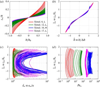
Sample profiles: of buoyancy (a,b); effective diffusivity (c); and characteristic Péclet number
 $\mathit{Pe}_{\ast }$
, as defined in (4.6) (d). Multiple profiles are plotted for each simulation as the profiles evolve in time. Profiles are shown for: simulation 6, an
 $\mathsf{L}$
state with
 $(\mathit{Pr},\mathit{Re})=(0.7,4250)$
(plotted in red); simulation 12, an
 $\mathsf{L}$
state with
 $(\mathit{Pr},\mathit{Re})=(7,4250)$
(plotted in green); simulation 17, an
 $\mathsf{L}$
state with
 $(\mathit{Pr},\mathit{Re})=(7,14\,700)$
(plotted in magenta); and simulation 16, an
 $\mathsf{H}$
state with
 $(\mathit{Pr},\mathit{Re})=(70,4250)$
(plotted in blue). In (b) the vertical extent of the buoyancy profile is rescaled by the interface thickness
 $\unicode[STIX]{x1D6FF}_{\ast }$
defined in (4.1) and its magnitude is rescaled by the buoyancy difference across the interface
 $\unicode[STIX]{x0394}b$
defined in (4.2).

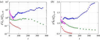
Time evolution of (a)
 $\unicode[STIX]{x2202}^{2}\hat{\unicode[STIX]{x1D705}}_{e}/\unicode[STIX]{x2202}\hat{z}_{\ast }^{2}$
and (b)
 $\unicode[STIX]{x2202}^{3}\hat{b}/\unicode[STIX]{x2202}\hat{z}_{\ast }^{3}$
at the midplane of the interface
 $\hat{z}_{\ast }=0$
. The colour conventions for the simulations are the same as those used in figure 8.

In order to examine the evolution of the buoyancy gradient governed by (4.5) it is necessary to evaluate the gradients with respect to the tracer-based coordinate
 $\hat{z}_{\ast }$
of the effective diffusivity
 $\hat{\unicode[STIX]{x1D705}}_{e}$
and the buoyancy
 $\hat{b}$
. However, the noise contained in the
 $\hat{z}_{\ast }$
profiles associated with sampling issues (as shown in figure 8) tends to get amplified if finite differences are taken repeatedly on the
 $\hat{z_{\ast }}$
profiles to obtain the
 $\unicode[STIX]{x2202}^{2}/\unicode[STIX]{x2202}\hat{z}_{\ast }^{2}$
and
 $\unicode[STIX]{x2202}^{3}/\unicode[STIX]{x2202}\hat{z}_{\ast }^{3}$
gradients associated with higher-order derivatives. Instead, we obtain an estimate of these gradients by first fitting polynomial functions to the observed
 $\hat{\unicode[STIX]{x1D705}}_{e}(\hat{z}_{\ast })$
and
 $\hat{b}(\hat{z}_{\ast })$
profiles using a nonlinear least squares algorithm and then calculate the gradients based on these fitted polynomial functions. Taking into account the symmetry of the profiles about the midplane
 $\hat{z}_{\ast }=0$
, we assume that
 $\hat{\unicode[STIX]{x1D705}}_{e}$
follows a parabolic profile
 $\hat{\unicode[STIX]{x1D705}}_{e}=c_{1}+c_{2}\hat{z}_{\ast }^{2}$
and that
 $\hat{b}$
follows a cubic profile
 $\hat{b}=c_{3}\hat{z}_{\ast }+c_{4}\hat{z}_{\ast }^{3}$
. It is worth noting that the rescaled buoyancy profiles
 $\hat{b}$
collapse reasonably well as shown in figure 8(b).
The gradients of
 $\hat{b}$
with respect to
 $\hat{z}_{\ast }$
are
 $O(1)$
and they do not vary significantly from one simulation to another, as shown for example in figure 9. On the other hand, the gradients of
 $\hat{\unicode[STIX]{x1D705}}_{e}$
vary strongly between the various simulations. This can be seen in figure 8(c) where the rescaled
 $\hat{\unicode[STIX]{x1D705}}_{e}(\hat{z}_{\ast })$
profiles do not collapse. The curvature of the
 $\hat{\unicode[STIX]{x1D705}}_{e}(\hat{z}_{\ast })$
profile, i.e.
 $\unicode[STIX]{x2202}^{2}\hat{\unicode[STIX]{x1D705}}_{e}/\unicode[STIX]{x2202}\hat{z}_{\ast }^{2}$
, varies significantly between the various simulations and varies strongly in time, as is shown in figure 9(a).
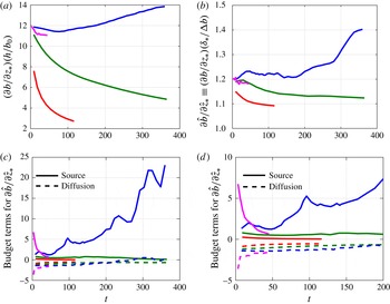
(a,b) Time evolution of the buoyancy gradient
 $N_{\ast }^{2}\equiv \unicode[STIX]{x2202}b/\unicode[STIX]{x2202}z_{\ast }$
at the midplane of the interface
 $z_{\ast }=0$
. In (a) the gradient is scaled by
 $b_{0}/h$
, and in (b) the local scaling
 $\unicode[STIX]{x0394}b/\unicode[STIX]{x1D6FF}_{\ast }$
is used. (c) Time evolution of the source term
 $\hat{\mathbb{S}}(t)$
(solid lines) and the diffusion term
 $\hat{\mathbb{D}}(t)$
(dashed lines), as defined in (4.5), for
 $z_{\ast }=0$
. (d) A zoomed view of (c) for
 $t<200$
. Data are shown for: simulation 6 with
 $(\mathit{Pr},\mathit{Re})=(0.7,4250)$
(plotted in red); simulation 12 with
 $(\mathit{Pr},\mathit{Re})=(7,4250)$
(plotted in green); simulation 17 with
 $(\mathit{Pr},\mathit{Re})=(7,14\,700)$
(plotted in magenta); and simulation 16 with
 $(\mathit{Pr},\mathit{Re})=(70,4250)$
(plotted in blue), i.e. the same colour conventions as those used in figure 8.

In figures 10(a,b), the time evolution of the buoyancy gradient at the midplane
 $z_{\ast }=0$
is shown for the four simulations with
 $\mathit{Ri}=0.32$
. Except for simulation 16 which is in the
 $\mathsf{H}$
state, the gradient decreases with time for simulations 6, 12 and 17, all of which are in the
 $\mathsf{L}$
state. In simulation 16 the density interface is maintained and the gradient at
 $z_{\ast }=0$
is weakly enhanced due to ‘scouring’ motions (see figure 4
b). The time series of the source and diffusion terms in (4.5) which govern the time evolution of the local gradient
 $\unicode[STIX]{x2202}\hat{b}/\unicode[STIX]{x2202}\hat{z}_{\ast }$
are shown in figures 10(c,d). At the midplane of the interface, the advection term
 $\hat{\mathbb{A}}(t)$
is expected to be zero as both
 $\unicode[STIX]{x1D705}_{e}$
and
 $\unicode[STIX]{x2202}b/\unicode[STIX]{x2202}z_{\ast }$
reach local extrema at
 $z_{\ast }=0$
due to symmetry (see figure 7). While for all simulations shown the source term
 $\hat{\mathbb{S}}(t)$
takes positive values, i.e. there is ‘scouring’ acting on the interface in all these cases, only in simulation 16 is this source term large enough to overcome the diffusion term
 $\hat{\mathbb{D}}(t)$
, causing the local gradient
 $\unicode[STIX]{x2202}\hat{b}/\unicode[STIX]{x2202}\hat{z}_{\ast }$
to be enhanced. In the laminarising state cases, (simulations 6, 12 and 17) however, the scouring effect is weak compared to the molecular diffusion which is characterised by the
 $\hat{\mathbb{D}}(t)$
term.
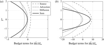
Variation with
 $\hat{z}_{\ast }$
of the various bracketed budget terms defined in (4.5) for: (a) a representative ‘diffusing’ interface in simulation 12 at
 $t\approx 100$
; (b) a representative ‘sharpening’ interface in simulation 16 at
 $t\approx 200$
.

In figure 11 we examine the
 $\hat{z}_{\ast }$
-dependence of the budget terms in (4.5) for a ‘diffusing’ interface in an
 $\mathsf{L}$
state simulation (simulation 12) for which the midplane gradient decreases (figure 11
a) and a ‘sharpening’ interface in an
 $\mathsf{H}$
state simulation (simulation 16) for which the midplane gradient increases (figure 11
b) respectively. In both cases, the advection term
 $\hat{\mathbb{A}}$
and the diffusion term
 $\hat{\mathbb{D}}$
both reduce the local gradient. In order for sharpening to occur, the source term
 $\hat{\mathbb{S}}$
has to outweigh
 $\hat{\mathbb{A}}$
and
 $\hat{\mathbb{D}}$
, which is the case shown in figure 11(b). Note also that the enhancement of local gradients can only occur over a finite extent in
 $\hat{z}_{\ast }$
, i.e. sharpening around the centre of the interface comes at the expense of the buoyancy gradient immediately above and below the midplane at
 $\hat{z}_{\ast }=0$
.
4.3 Effect of Péclet number and isopycnal displacement
The terms
 $\unicode[STIX]{x2202}\hat{b}/\unicode[STIX]{x2202}\hat{z}_{\ast }$
,
 $\hat{\unicode[STIX]{x1D705}}_{e}$
and
 $\unicode[STIX]{x2202}^{3}\hat{b}/\unicode[STIX]{x2202}\hat{z}_{\ast }^{3}$
which appear in the source and diffusion terms in (4.5) are all of order unity at the midplane
 $z_{\ast }=0$
, as can be seen in figures 8(c), 9 and 10(b), respectively. Therefore, in order for
 $\hat{\mathbb{S}}$
to dominate
 $\hat{\mathbb{D}}$
, the
 $\unicode[STIX]{x2202}^{2}\hat{\unicode[STIX]{x1D705}}_{e}/\unicode[STIX]{x2202}\hat{z}_{\ast }^{2}$
term needs to be at least of order unity or larger. In figure 12, the values of
 $\unicode[STIX]{x2202}^{2}\hat{\unicode[STIX]{x1D705}}_{e}/\unicode[STIX]{x2202}\hat{z}_{\ast }^{2}$
sampled at
 $z_{\ast }=0$
are plotted against the characteristic Péclet number of the flow. The characteristic Péclet number, which is a function of
 $z_{\ast }$
and
 $t$
, is defined as
 $$\begin{eqnarray}\mathit{Pe}_{\ast }(z_{\ast },t)\equiv \frac{{\mathcal{U}}_{\ast }(z_{\ast },t){\mathcal{L}}_{\ast }(z_{\ast },t)}{\unicode[STIX]{x1D705}},\end{eqnarray}$$
where the characteristic turbulent velocity scale is defined as
 $$\begin{eqnarray}{\mathcal{U}}_{\ast }\equiv \sqrt{\langle u^{\prime 2}+v^{\prime 2}+w^{\prime 2}\rangle _{z_{\ast }}},\end{eqnarray}$$
and the characteristic length scale is defined as
 $$\begin{eqnarray}{\mathcal{L}}_{\ast }\equiv \frac{{\mathcal{U}}_{\ast }}{\sqrt{\unicode[STIX]{x1D700}_{\ast }/\unicode[STIX]{x1D708}}}.\end{eqnarray}$$
In the definition above,
 $\unicode[STIX]{x1D700}_{\ast }\equiv \langle 2\unicode[STIX]{x1D708}\unicode[STIX]{x1D634}_{ij}\unicode[STIX]{x1D634}_{ij}\rangle _{z_{\ast }}$
is the kinetic energy dissipation rate averaged for a given reference position
 $z_{\ast }$
, and
 $\unicode[STIX]{x1D634}_{ij}$
is the rate of strain tensor associated with the full velocity field
 $\boldsymbol{u}$
. The definition of the length scale
 ${\mathcal{L}}_{\ast }$
is analogous to the Taylor microscale which is often used to describe isotropic turbulence (see e.g. Pope Reference Pope2000). The quantities
 ${\mathcal{U}}_{\ast }$
and
 ${\mathcal{L}}_{\ast }$
can be considered to be the characteristic velocity and length scales corresponding to the ‘scouring’ motion, and
 $\mathit{Pe}_{\ast }$
measures the relative magnitude of scouring over molecular diffusion.
 $\mathit{Pe}_{\ast }$
tends to increase weakly away from the midplane
 $z_{\ast }=0$
as shown in figure 8(d).
Variation of the curvature of the
 $\hat{\unicode[STIX]{x1D705}}_{e}$
profile, i.e.
 $\unicode[STIX]{x2202}^{2}\hat{\unicode[STIX]{x1D705}}_{e}/\unicode[STIX]{x2202}\hat{z}_{\ast }^{2}$
, at the midplane of the interface
 $\hat{z}_{\ast }=0$
, with the characteristic Péclet number
 $\overline{\mathit{Pe}}_{\ast }$
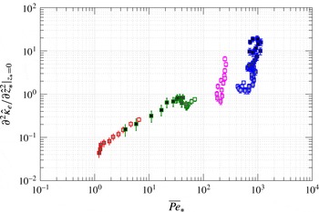
. The colour conventions for the simulations are the same as in figure 8. Darker filling colours of symbols correspond to later times in each simulation.

As is plotted in figure 12, the magnitude of
 $\unicode[STIX]{x2202}^{2}\hat{\unicode[STIX]{x1D705}}_{e}/\unicode[STIX]{x2202}\hat{z}_{\ast }^{2}$
increases strongly with
 $\overline{\mathit{Pe}}_{\ast }$
, the depth-averaged Péclet number of a given profile, where the overline indicates an average as defined in (4.3). This figure illustrates the fact that
 $\hat{\unicode[STIX]{x1D705}}_{e}$
profiles exhibit more curvature as the effects of scouring become increasingly more important than molecular diffusion. Significantly, the curvature does not appear to vary systemically with other characteristic flow parameters such as buoyancy Reynolds number and local gradient Richardson number (as discussed in § 5), the magnitude of which vary little across the four simulations shown in figure 12. The magnitude of
 $\unicode[STIX]{x2202}^{2}\hat{\unicode[STIX]{x1D705}}_{e}/\unicode[STIX]{x2202}\hat{z}_{\ast }^{2}$
becomes larger than order unity for simulation 16 (plotted in blue) with
 $\overline{\mathit{Pe}}_{\ast }\gtrsim 400$
. As the flow evolves in this simulation (the filling colour of the symbol is darker for later times), both
 $\overline{\mathit{Pe}}_{\ast }$
and
 $\unicode[STIX]{x2202}^{2}\hat{\unicode[STIX]{x1D705}}_{e}/\unicode[STIX]{x2202}\hat{z}_{\ast }^{2}$
increase with time. Other simulations with
 $\overline{\mathit{Pe}}_{\ast }\lesssim 300$
do not have curvature
 $\unicode[STIX]{x2202}^{2}\hat{\unicode[STIX]{x1D705}}_{e}/\unicode[STIX]{x2202}\hat{z}_{\ast }^{2}$
maintained at values larger than order unity. Although in simulation 17 (plotted in magenta) the
 $\unicode[STIX]{x2202}^{2}\hat{\unicode[STIX]{x1D705}}_{e}/\unicode[STIX]{x2202}\hat{z}_{\ast }^{2}$
value starts with magnitude of order unity, it decays with time as the flow laminarises. It appears that there exists a transitional
 $\overline{\mathit{Pe}}_{\ast }$
between 300 and 400 above which the scouring is able to overcome diffusion so that the curvature in
 $\hat{\unicode[STIX]{x1D705}}_{e}$
can be maintained or enhanced.
This observation is reminiscent of the grid-stirred experiments (Crapper & Linden Reference Crapper and Linden1974). In that paper, the behaviour of a density interface in the absence of mean shear is reported to vary significantly depending on whether an appropriate Péclet number is ‘large’ or ‘small’, i.e. whether the Péclet number based on the turbulent velocity and length scales at the interface is above or below approximately 200. For the highly stable, vertically sheared interfaces we examine here, the magnitude of the Péclet number also appears to determine whether or not the scouring motion, which acts to sustain the interface, can overcome molecular diffusion, which acts to smooth the sharp gradient.
We also examine the weak enhancement of the effective diffusivity
 $\unicode[STIX]{x1D705}_{e}$
relative to the molecular diffusivity
 $\unicode[STIX]{x1D705}$
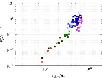
in the simulations of very stable interfaces. Figure 13 shows the depth-averaged enhancement ratio of effective diffusivity,
 $\overline{\unicode[STIX]{x1D705}_{e}}/\unicode[STIX]{x1D705}-1$
, plotted against the ratio of the Ellison length scale to the integral thickness of the interface,
 $\overline{\ell _{E,\ast }}/\unicode[STIX]{x1D6FF}_{\ast }$
, (a measure of the vertical isopycnal displacements) where the Ellison length scale is defined as
 $$\begin{eqnarray}\ell _{E,\ast }(z_{\ast },t)\equiv \frac{\sqrt{\langle b^{\prime 2}\rangle _{z_{\ast }}}}{\unicode[STIX]{x2202}\langle b\rangle _{z_{\ast }}/\unicode[STIX]{x2202}z_{\ast }},\end{eqnarray}$$
and
 $b^{\prime }\equiv b-\langle b\rangle$
denotes the buoyancy fluctuation relative to the horizontal mean
 $\langle b\rangle$
. Figure 13 suggests that the moderate increase in
 $\unicode[STIX]{x1D705}_{e}$
relative to
 $\unicode[STIX]{x1D705}$
within the density interface is strongly correlated to the magnitude of isopycnal displacements. This observation reinforces the notion, which is encapsulated in (3.4), that diapycnal mixing is made more effective by a flow which creates larger isopycnal surface area for transport by molecular flux. In particular, enhancement of diffusion is achieved by the corrugation of isopycnal surfaces due to scouring motions acting on the very stable interfaces, an effect that is expected to be more significant as the isopycnal displacements increase in amplitude.
Variation of the depth-averaged enhancement ratio of diffusivity
 $\unicode[STIX]{x1D705}_{e}/\unicode[STIX]{x1D705}-1$
with the depth-averaged (across the interface) length scale ratio
 $\overline{\ell _{E,\ast }}/\unicode[STIX]{x1D6FF}_{\ast }$
. The colour conventions for the simulations are the same as in figure 8. Darker filling colours of symbols correspond to later times in each simulation.

5 Mixing analysis in the tracer-based coordinate
5.1 Scaling of effective diffusivity
In this section, we consider the variation of irreversible mixing properties with characteristic flow parameters in all three flow states,
 $\mathsf{L}$
,
 $\mathsf{H}$
and
 $\mathsf{T}$
. We start by investigating the effective diffusivity
 $\unicode[STIX]{x1D705}_{e}$
as defined by (3.1). Following the Winters–D’Asaro–Nakamura formalism,
 $\unicode[STIX]{x1D705}_{e}$
values are sampled locally at each
 $z_{\ast }$
using (3.3). All data points considered here are for
 $z_{\ast }$
locations sampled over the entire depth of the channel, i.e.
 $-h<z_{\ast }<h$
and for
 $t>10$
advective time units when the flow is observed to be free from initial transient effects due to the sudden introduction of the density interface at
 $t=0$
. The values of
 $\unicode[STIX]{x1D705}_{e}$
, normalised by molecular kinematic viscosity
 $\unicode[STIX]{x1D708}$
, are plotted against the locally sampled buoyancy Reynolds number
 $\mathit{Re}_{b,\ast }$
and gradient Richardson number
 $\mathit{Ri}_{g,\ast }$
, respectively, in figure 14. Specifically,
 $\mathit{Re}_{b,\ast }$
and
 $\mathit{Ri}_{g,\ast }$
are defined in the tracer-based reference coordinate
 $z_{\ast }$
by
 $$\begin{eqnarray}\mathit{Re}_{b,\ast }(z_{\ast },t)\equiv \frac{\unicode[STIX]{x1D700}_{\ast }}{\unicode[STIX]{x1D708}N_{\ast }^{2}}\quad \text{and}\quad \mathit{Ri}_{g,\ast }(z_{\ast },t)\equiv \frac{N_{\ast }^{2}}{S_{\ast }^{2}},\end{eqnarray}$$
where
 $S_{\ast }\equiv \langle \unicode[STIX]{x2202}u/\unicode[STIX]{x2202}z\rangle _{z_{\ast }}$
is the averaged vertical shear of streamwise velocity sampled over a given
 $z_{\ast }$
position.
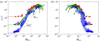
Variation of normalised
 $\unicode[STIX]{x1D705}_{e}(z_{\ast },t)/\unicode[STIX]{x1D708}$
with: (a)
 $\mathit{Re}_{b,\ast }(z_{\ast },t)$
; and (b)
 $\mathit{Ri}_{g,\ast }(z_{\ast },t)$
. Horizontal dashed lines in (a) correspond to
 $\unicode[STIX]{x1D705}_{e}/\unicode[STIX]{x1D708}=\unicode[STIX]{x1D705}/\unicode[STIX]{x1D708}=1/\mathit{Pr}$
for
 $\mathit{Pr}=0.7$
(red), 7 (green or magenta) and 70 (blue) respectively. Symbol conventions are listed in table 1.

Figure 14(a) indicates a clear dependence of
 $\unicode[STIX]{x1D705}_{e}/\unicode[STIX]{x1D708}$
on both
 $\mathit{Re}_{b,\ast }$
and
 $\mathit{Pr}$
at least for
 $\mathit{Re}_{b,\ast }<100$
. For
 $\mathit{Re}_{b,\ast }=O(1)$
or smaller,
 $\unicode[STIX]{x1D705}_{e}$
approaches the value
 $\unicode[STIX]{x1D705}$
, i.e.
 $\unicode[STIX]{x1D705}_{e}/\unicode[STIX]{x1D708}\rightarrow 1/\mathit{Pr}$
, in this ‘molecular’ regime (see e.g. Shih et al.
Reference Shih, Koseff, Ivey and Ferziger2005; Bouffard & Boegman Reference Bouffard and Boegman2013). For
 $O(1)<\mathit{Re}_{b,\ast }\lesssim 30$
, the scaling enters a ‘buoyancy-controlled’ regime where
 $\unicode[STIX]{x1D705}_{e}/\unicode[STIX]{x1D708}\propto \mathit{Re}_{b,\ast }^{3/2}$
(cf. Bouffard & Boegman (Reference Bouffard and Boegman2013) and the references therein). Consistent with Bouffard & Boegman (Reference Bouffard and Boegman2013), for a given
 $\mathit{Re}_{b,\ast }$
value
 $\unicode[STIX]{x1D705}_{e}/\unicode[STIX]{x1D708}$
decreases with increasing
 $\mathit{Pr}$
. For
 $30\lesssim \mathit{Re}_{b,\ast }\lesssim 100$
, i.e. the ‘transitional’ regime,
 $\unicode[STIX]{x1D705}_{e}/\unicode[STIX]{x1D708}$
is proportional to
 $\mathit{Re}_{b,\ast }$
, which agrees with the scaling of this regime described by Shih et al. (Reference Shih, Koseff, Ivey and Ferziger2005), although it is important to remember that the specific numerical values of the buoyancy Reynolds number depend on the choices for dissipation rate and buoyancy frequency made, which can of course vary between different analyses.
Within this ‘transitional’ regime, the weak dependence of
 $\unicode[STIX]{x1D705}_{e}/\unicode[STIX]{x1D708}$
on
 $\mathit{Pr}$
can still be observed in our data. A simple power-law relation for
 $\unicode[STIX]{x1D705}_{e}/\unicode[STIX]{x1D708}$
in terms of
 $\mathit{Re}_{b,\ast }$
is not identifiable for
 $\mathit{Re}_{b,\ast }\gtrsim 100$
and the
 $\mathit{Pr}$
dependence is also less distinct. Figure 14(b) shows the variation of
 $\unicode[STIX]{x1D705}_{e}/\unicode[STIX]{x1D708}$
with
 $\mathit{Ri}_{g,\ast }$
where the reverse trend in
 $\mathit{Re}_{b,\ast }$
can be observed, i.e.
 $\unicode[STIX]{x1D705}_{e}/\unicode[STIX]{x1D708}$
in general decreases with increasing
 $\mathit{Ri}_{g,\ast }$
. This reversed trend is because, as will be shown in figure 18,
 $\mathit{Re}_{b,\ast }$
and
 $\mathit{Ri}_{g,\ast }$
are inversely correlated to each other in these simulations. The degree of scatter is greater in the
 $\mathit{Ri}_{g,\ast }$
plot than in the
 $\mathit{Re}_{b,\ast }$
plot.
We now turn our attention to the
 $\mathit{Re}_{b,\ast }\gtrsim 100$
regime, where simple power laws in
 $\mathit{Re}_{b,\ast }$
do not appear to describe the data, as is shown in figure 14(a). These large
 $\mathit{Re}_{b,\ast }$
values are observed exclusively in the
 $\mathsf{T}$
state where the flow remains turbulent despite the introduction of the density interface and approaches a fully developed turbulent state (Zhou et al.
Reference Zhou, Taylor and Caulfield2017). In a fully turbulent stratified plane Couette flow, diapycnal mixing is characterised by a linear relation between the flux and gradient Richardson numbers, i.e. the turbulent Prandtl number
 $\mathit{Pr}_{t}\equiv \mathit{Ri}_{f}/\mathit{Ri}_{g}$
is close to unity, where
 $\mathit{Ri}_{f}$
is the flux Richardson number defined as the ratio of buoyancy flux and shear production. In other words, this is the typical behaviour on the weakly stratified ‘left flank’ of Phillips’ flux-gradient curve (see figure 1). This results in a scaling of
 $\unicode[STIX]{x1D705}_{e}/\unicode[STIX]{x1D708}=\mathit{Re}_{b}\mathit{Ri}_{g}/(1-\mathit{Ri}_{g})$
(Zhou et al.
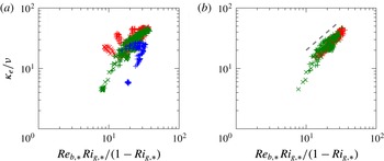
Reference Zhou, Taylor and Caulfield2017) which is tested in figure 15. In (a) some large deviations from this ‘left-flank’ scaling can be observed, as the data points plotted include early time points (
 $t<60$
) where the interface is undergoing shear-induced overturns. As the transition to stronger turbulence is close to completion at
 $t>60$
, the
 $\unicode[STIX]{x1D705}_{e}/\unicode[STIX]{x1D708}$
follows more closely the ‘left-flank’ scaling
 $Ri_{f}\simeq \mathit{Ri}_{g}$
for equilibrated weakly stratified shear flows, as shown for example in figure 13 of Deusebio et al. (Reference Deusebio, Caulfield and Taylor2015).
Application of the weakly stratified ‘left-flank’ scaling, i.e.
 $\unicode[STIX]{x1D705}_{e}/\unicode[STIX]{x1D708}=\mathit{Re}_{b}\mathit{Ri}_{g}/(1-\mathit{Ri}_{g})$
, proposed for fully developed stratified plane Couette flow (Zhou et al.
Reference Zhou, Taylor and Caulfield2017), to the layered stratified plane Couette flow data. The ‘left-flank’ data points, with small bulk Richardson numbers
 $\mathit{Ri}\leqslant 0.02$
are shown in (a) for
 $t>10$
and (b) for
 $t>60$
. Dashed line in (b) indicates one-to-one slope. Symbol conventions are listed in table 1.

5.2 Scaling of volume-integrated mixing efficiency
In this subsection, we consider the mixing efficiency of a density interface in the volume-integrated sense. The framework of the analysis focusing on the available potential energy change in a control volume was proposed originally by Winters et al. (Reference Winters, Lombard, Riley and D’Asaro1995) and was employed subsequently to characterise the irreversible mixing efficiency in a given system by e.g. Caulfield & Peltier (Reference Caulfield and Peltier2000), Peltier & Caulfield (Reference Peltier and Caulfield2003). Here, we focus on the region within the density interface where a significant buoyancy gradient,
 $N_{\ast }^{2}$
, is present and consider the integrated mixing properties over an interval in the
 $z_{\ast }$
coordinate with
 $-\unicode[STIX]{x1D6FF}_{\ast }<z_{\ast }<\unicode[STIX]{x1D6FF}_{\ast }$
, where
 $\unicode[STIX]{x1D6FF}_{\ast }$
is the integral thickness of the interface in the
 $z_{\ast }$
coordinate as defined by (4.1). The integrated diapycnal flux is
 $$\begin{eqnarray}\unicode[STIX]{x1D6F7}_{d}(t)\equiv -\overline{\unicode[STIX]{x1D719}}_{d}\cdot 2\unicode[STIX]{x1D6FF}_{\ast }=\int _{-\unicode[STIX]{x1D6FF}_{\ast }}^{\unicode[STIX]{x1D6FF}_{\ast }}-\unicode[STIX]{x1D719}_{d}(z_{\ast },t)\,\text{d}z_{\ast }=\int _{-\unicode[STIX]{x1D6FF}_{\ast }}^{\unicode[STIX]{x1D6FF}_{\ast }}\unicode[STIX]{x1D705}_{e}\frac{\unicode[STIX]{x2202}b}{\unicode[STIX]{x2202}z_{\ast }}\,\text{d}z_{\ast },\end{eqnarray}$$
and the integrated dissipation is
 $$\begin{eqnarray}{\mathcal{E}}(t)\equiv \int _{-\unicode[STIX]{x1D6FF}_{\ast }}^{\unicode[STIX]{x1D6FF}_{\ast }}\unicode[STIX]{x1D700}_{\ast }(z_{\ast },t)\,\text{d}z_{\ast }.\end{eqnarray}$$
The overall irreversible mixing efficiency across the interface, which is defined as
 $$\begin{eqnarray}E_{tot}(t)\equiv \frac{\unicode[STIX]{x1D6F7}_{d}}{\unicode[STIX]{x1D6F7}_{d}+{\mathcal{E}}},\end{eqnarray}$$
can then be estimated. In addition, it is possible to define a measure of mixing efficiency which excludes the laminar diffusion of the background profile with the laminar flux
 $\unicode[STIX]{x1D719}_{d,lam}\equiv -(\unicode[STIX]{x2202}b/\unicode[STIX]{x2202}z_{\ast })\unicode[STIX]{x1D705}$
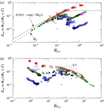
, following the suggestion of Caulfield & Peltier (Reference Caulfield and Peltier2000) in an attempt to isolate the irreversible mixing inherently due to turbulent mixing processes. The corresponding integrated diapycnal flux is
 $$\begin{eqnarray}{\mathcal{M}}(t)\equiv \int _{-\unicode[STIX]{x1D6FF}_{\ast }}^{\unicode[STIX]{x1D6FF}_{\ast }}-(\unicode[STIX]{x1D719}_{d}-\unicode[STIX]{x1D719}_{d,lam})\,\text{d}z_{\ast }=\int _{-\unicode[STIX]{x1D6FF}_{\ast }}^{\unicode[STIX]{x1D6FF}_{\ast }}(\unicode[STIX]{x1D705}_{e}-\unicode[STIX]{x1D705})\frac{\unicode[STIX]{x2202}b}{\unicode[STIX]{x2202}z_{\ast }}\,\text{d}z_{\ast },\end{eqnarray}$$
and the corresponding ‘turbulent’ mixing efficiency is
 $$\begin{eqnarray}E(t)\equiv \frac{{\mathcal{M}}}{{\mathcal{M}}+{\mathcal{E}}}.\end{eqnarray}$$
Variation of the time-dependent total mixing efficiency
 $E_{tot}\equiv \unicode[STIX]{x1D6F7}_{d}/(\unicode[STIX]{x1D6F7}_{d}+{\mathcal{E}})$
across the density interface
 $-\unicode[STIX]{x1D6FF}_{\ast }<z_{\ast }<\unicode[STIX]{x1D6FF}_{\ast }$
with the corresponding depth averaged: (a)
 $\overline{\mathit{Ri}}_{g,\ast }$
; and (b)
 $\overline{\mathit{Re}}_{b,\ast }$
. Darker filling colours for the closed symbols and thicker lines for open symbols correspond to later times in each simulation. Symbol conventions are shown in table 1. Grey open squares in (b) correspond to data from Shih et al. (Reference Shih, Koseff, Ivey and Ferziger2005) with
 $\mathit{Pr}=0.72$
. In (a), a dashed line shows the relation
 $E_{tot}=\overline{\mathit{Ri}}_{g,\ast }$
, and a dashed-dotted line shows the relation proposed by Venayagamoorthy & Koseff (Reference Venayagamoorthy and Koseff2016),
 $E_{tot}=0.25[1-\exp (-7\cdot \overline{\mathit{Ri}}_{g,\ast })]$
.

Variation of the time-dependent turbulent mixing efficiency
 $E\equiv {\mathcal{M}}/({\mathcal{M}}+{\mathcal{E}})$
across the density interface
 $-\unicode[STIX]{x1D6FF}_{\ast }<z_{\ast }<\unicode[STIX]{x1D6FF}_{\ast }$
with the corresponding depth averaged: (a)
 $\overline{\mathit{Ri}}_{g,\ast }$
; and (b)
 $\overline{\mathit{Re}}_{b,\ast }$
. Darker filling colours for the closed symbols and thicker lines for open symbols correspond to later times in each simulation. Symbol conventions are shown in table 1.

Figure 16 shows the total (turbulent and molecular) mixing efficiency
 $E_{tot}$
as a function of depth-averaged gradient Richardson number
 $\overline{\mathit{Ri}}_{g,\ast }$
and buoyancy Reynolds number
 $\overline{\mathit{Re}}_{b,\ast }$
, where the overbar indicates an average defined by (4.3). As shown in (a),
 $E_{tot}$
increases with
 $\overline{\mathit{Ri}}_{g,\ast }$
for
 $\overline{\mathit{Ri}}_{g,\ast }\lesssim 0.1$
corresponding to the
 $\mathsf{T}$
state. The relation
 $E_{tot}=\mathit{Ri}_{g}$
plotted with a dashed line is equivalent to setting the turbulent Prandtl number
 $\mathit{Pr}_{t}=1$
, which appears to agree well with the data showing the typical ‘left-flank’ behaviour in the Phillips flux-gradient curve (figure 1). The data enter the ‘right-flank’ regime for
 $\overline{\mathit{Ri}}_{g,\ast }\gtrsim 0.1$
where
 $E_{tot}$
is observed to vary strongly with the molecular Prandtl number
 $\mathit{Pr}$
. Data points in this regime correspond mainly to the
 $\mathsf{L}$
and
 $\mathsf{H}$
states. Specifically, for
 $\mathit{Pr}=0.7$
(plotted in red)
 $E_{tot}$
continues to increase with
 $\overline{\mathit{Ri}}_{g,\ast }$
, because laminar diffusion, at least for these simulations, becomes important immediately after the flow enters the strongly stratified right flank. Non-monotonic behaviour of
 $E_{tot}$
in
 $\overline{\mathit{Ri}}_{g,\ast }$
is observed for
 $\mathit{Pr}=7$
(plotted in green) and
 $70$
(plotted in blue) where
 $E_{tot}$
first decreases with
 $\overline{\mathit{Ri}}_{g,\ast }$
and increases again when
 $\overline{\mathit{Ri}}_{g,\ast }$
becomes sufficiently large due to the strength of the buoyancy gradient
 $\unicode[STIX]{x2202}b/\unicode[STIX]{x2202}z_{\ast }$
. Shown also in figure 16(a) is the relation between
 $E_{tot}$
and
 $\overline{\mathit{Ri}}_{g,\ast }$
proposed by Venayagamoorthy & Koseff (Reference Venayagamoorthy and Koseff2016) plotted with a dashed-dotted line. While the relation is reasonably close to the data on the left flank,
 $E_{tot}$
does not asymptote to a constant value of 0.25 as is predicted to occur in a linearly stratified system by Venaille et al. (Reference Venaille, Gostiaux and Sommeria2017), although as usual, it is important to remember that the definitions of mixing efficiency and Richardson number vary between analyses, and indeed the mechanisms by which energy is injected into the flow also vary markedly.
When plotted against
 $\overline{\mathit{Re}}_{b,\ast }$
, as is shown in figure 16(b),
 $E_{tot}$
appears to collapse into single curves for each value of
 $\mathit{Pr}$
. For
 $\mathit{Re}_{b,\ast }\lesssim 100$
,
 $E_{tot}$
takes larger values for smaller
 $\mathit{Pr}$
at a given
 $\mathit{Re}_{b,\ast }$
, and for
 $\mathit{Re}_{b,\ast }\gtrsim 100$
, the dependence on
 $\mathit{Pr}$
seems to disappear. Consistent with Shih et al. (Reference Shih, Koseff, Ivey and Ferziger2005),
 $E_{tot}$
decreases with
 $\overline{\mathit{Re}}_{b,\ast }$
for
 $\mathit{Re}_{b,\ast }\gtrsim 100$
. The Shih et al. (Reference Shih, Koseff, Ivey and Ferziger2005) data of
 $\mathit{Pr}=0.72$
(plotted as grey squares) show consistency with the LSPC data for simulations with
 $\mathit{Pr}=0.7$
(plotted in red) for
 $\mathit{Re}_{b,\ast }>O(1)$
.
Figure 17 shows the time-dependent ‘turbulent’ mixing efficiency
 $E$
as a function of
 $\overline{\mathit{Ri}}_{g,\ast }$
and
 $\overline{\mathit{Re}}_{b,\ast }$
. Interestingly, in figure 17(a) where
 $E$
is plotted against
 $\overline{\mathit{Ri}}_{g,\ast }$
, the strong dependence on
 $\mathit{Pr}$
on the ‘right flank’ with
 $\overline{\mathit{Ri}}_{g,\ast }\gtrsim 0.1$
vanishes when the laminar diffusion is excluded. As the flow further laminarises in the
 $\mathsf{L}$
state,
 $E$
decreases with time (as shown by increasingly darker symbol fill colour). For the
 $\mathsf{H}$
state plotted in blue squares, however, the efficiency
 $E$
saturates to a value between
 $10^{-3}$
and
 $10^{-2}$
. The same observation applies to the ‘left flank’ in
 $\overline{\mathit{Re}}_{b,\ast }$
as shown in figure 17(b). The behaviour of
 $E$
follows closely that of
 $E_{tot}$
shown in figure 16 for
 $\overline{\mathit{Ri}}_{g,\ast }\lesssim 0.1$
, as the contribution of laminar diffusion is negligible in flows where turbulent transport dominates, as expected. The data shown in (a) are also reminiscent of the results compiled by Fernando (Reference Fernando1991) in his figure 16, although, again it is important to remember that the definitions of ‘Richardson number’ are different.
It is also important to appreciate the causes of the differences between the total mixing efficiency
 $E_{tot}$
(figure 16) and the turbulent mixing efficiency
 $E$
(figure 17). The definition
 $E$
removing the purely diffusive component was proposed by Caulfield & Peltier (Reference Caulfield and Peltier2000) based on the assumption that the dominant mixing properties in flows unstable to KHI are associated with the breakdown of the primary KHI billows. By their very character, KHI billows are large scale and dominated by inertial processes. As the Reynolds number of the flow increases, it is a reasonable hypothesis that the laminar ‘mixing’ dynamics will become increasingly insignificant. In the layered flow considered here, it is not at all clear that this assumption is valid, as even as the external
 $\mathit{Re}$
gets large, it is still expected that in the immediate vicinity of the density interface, diffusive ‘laminar’ dynamics will remain significant. This remaining significance is clearly implied by the spatial variation of
 $\unicode[STIX]{x1D705}_{e}$
in strongly layered flows as shown in figure 7.
5.3 Comparison to mixing associated with Kelvin–Helmholtz instabilities
Comparison with the dual-parameter scaling for turbulent mixing efficiency
 $E\equiv {\mathcal{M}}/({\mathcal{M}}+{\mathcal{E}})$
in
 $(\mathit{Ri}_{g},\mathit{Re}_{b})$
proposed by Salehipour et al. (Reference Salehipour, Peltier, Whalen and MacKinnon2016b
). In (a) the Salehipour et al. (Reference Salehipour, Peltier, Whalen and MacKinnon2016b
) predictions, denoted by
 $E_{KH}$
, are plotted as contours, and the points in the parameter space accessed by LSPC simulations are plotted in circles where the colour conventions follow table 1. The grey dashed line corresponds to where the maximum
 $E$
occurs for a given
 $\mathit{Ri}_{g}$
. The horizontal and vertical dashed-dotted lines correspond to
 $\mathit{Re}_{b}=20$
and
 $\mathit{Ri}_{g}=1/4$
respectively. The predicted
 $E_{KH}$
values are plotted against the LSPC results in (b) and (c) for
 $\mathit{Re}_{b}>20$
and
 $\mathit{Re}_{b}<20$
respectively. Darker fill colour corresponds to larger values of
 $\overline{\mathit{Re}}_{b,\ast }$
in (b) and larger values of
 $\overline{\mathit{Ri}}_{g,\ast }$
in (c). The dashed line in (c) and the insert plot corresponds to
 $E=E_{KH}$
.

In this section, we compare the mixing efficiency measured in our LSPC flows to the results obtained by simulating the turbulence induced by KHI, a canonical flow configuration often employed to study mixing, e.g. by Caulfield & Peltier (Reference Caulfield and Peltier2000), Smyth, Moum & Caldwell (Reference Smyth, Moum and Caldwell2001), Mashayek, Caulfield & Peltier (Reference Mashayek, Caulfield and Peltier2013) and Salehipour & Peltier (Reference Salehipour and Peltier2015). Figure 18 compares our LSPC data to a recent study by Salehipour et al. (Reference Salehipour, Peltier, Whalen and MacKinnon2016b
) which attempted to parameterise
 $E$
as a function of appropriate measures of gradient Richardson number and buoyancy Reynolds number based on data from direct numerical simulation of KHI. As previously noted, it is important to be cautious when comparing results from different analyses using different definitions of key parameters, and as described in detail in Salehipour & Peltier (Reference Salehipour and Peltier2015), the definitions of the gradient Richardson number and buoyancy Reynolds number used in Salehipour et al. (Reference Salehipour, Peltier, Whalen and MacKinnon2016b
) are somewhat different from those used here. To re-iterate, the
 $\overline{\mathit{Ri}}_{g,\ast }$
and
 $\overline{\mathit{Re}}_{b,\ast }$
values for our LSPC data are first calculated ‘locally’ as a function of
 $z_{\ast }$
using the definitions given in (5.1), and are then averaged using the ‘depth’ integral (denoted with an overbar) as defined in (4.3). As can be seen in figure 18(a),
 $\overline{\mathit{Ri}}_{g,\ast }$
and
 $\overline{\mathit{Re}}_{b,\ast }$
are strongly correlated to each other in the LSPC flows, i.e.
 $\overline{\mathit{Re}}_{b,\ast }$
tends to decrease with larger values of
 $\overline{\mathit{Ri}}_{g,\ast }$
. As a result, our data only access a subset of the parameter space. Interestingly, our data for
 $20\lesssim \mathit{Re}_{b}\lesssim 1000$
, which fall in the weakly stratified ‘left flank’ of the Phillips curve, follow closely the trajectory of maximum
 $E$
for a given
 $\overline{\mathit{Ri}}_{g,\ast }$
observed by Salehipour et al. (Reference Salehipour, Peltier, Whalen and MacKinnon2016b
). The LSPC data points do not access the most efficient regime observed by Salehipour et al. (Reference Salehipour, Peltier, Whalen and MacKinnon2016b
) when
 $\overline{\mathit{Re}}_{b,\ast }\gtrsim 20$
and
 $\overline{\mathit{Ri}}_{g,\ast }\gtrsim 0.25$
. For
 $\overline{\mathit{Re}}_{b,\ast }\gtrsim 20$
, the LSPC data agree reasonably well with Salehipour et al.’s (Reference Salehipour, Peltier, Whalen and MacKinnon2016b
) prediction
 $E_{KH}$
, as is shown in (b). The agreement, which seems to be improved for data of larger
 $\overline{\mathit{Re}}_{b,\ast }$
values, is presumably due to the fact that the underlying flow dynamics are similar in LSPC and KHI simulations for these data, i.e. shear-induced overturns dominate the diapycnal mixing in both cases. For the less energetic, more stratified data with
 $\overline{\mathit{Re}}_{b,\ast }\lesssim 20$
(or
 $\overline{\mathit{Ri}}_{g,\ast }\gtrsim 0.25$
), there is poor agreement between
 $E_{KH}$
and
 $E$
, as is shown in (c). The Salehipour et al. (Reference Salehipour, Peltier, Whalen and MacKinnon2016b
) scaling predicts larger efficiencies than those observed in the LSPC flow for small values of
 $\overline{\mathit{Ri}}_{g,\ast }\lesssim 1/2$
, as shown in the insert of (c). As
 $\overline{\mathit{Ri}}_{g,\ast }$
increases further to
 $\overline{\mathit{Ri}}_{g,\ast }\gtrsim 1/2$
,
 $E_{KH}$
becomes virtually zero, whereas
 $E$
stays at small but significantly non-zero values. This weak but non-negligible mixing occurs in
 $\mathsf{L}$
and
 $\mathsf{H}$
states at the right flank of the Phillips curve for which the diapycnal transport due to the scouring acting on a highly stable density interface plays a key role.
5.4 Comparison to body-forced turbulence mixing
(a) Turbulent mixing efficiency
 $E\equiv {\mathcal{M}}/({\mathcal{M}}+{\mathcal{E}})$
as a function of the depth-averaged horizontal Froude number
 $\overline{\mathit{Fr}}_{h,\ast }$
. The data from Maffioli et al. (Reference Maffioli, Brethouwer and Lindborg2016) are plotted as grey circles. (b)
 $\overline{\mathit{Ri}}_{g,\ast }$
as a function of
 $\overline{\mathit{Fr}}_{h,\ast }$
, where the dashed line corresponds to the
 $\mathit{Ri}_{g}\propto \mathit{Fr}_{h}^{-2}$
scaling for fully developed turbulent plane Couette flow (Zhou et al.
Reference Zhou, Taylor and Caulfield2017). Darker fill colour corresponds to larger values of
 $\mathit{Re}_{b}$
with samples shown in (a). Data points with
 $\overline{\mathit{Re}}_{b,\ast }>20$
are shown, consistent with the range investigated by Maffioli et al. (Reference Maffioli, Brethouwer and Lindborg2016).

Another highly relevant flow configuration in studying stratified turbulence is triply periodic forced turbulence simulations, e.g. by Brethouwer et al. (Reference Brethouwer, Billant, Lindborg and Chomaz2007). Here we also compare our results with a recent study by Maffioli et al. (Reference Maffioli, Brethouwer and Lindborg2016) who measured mixing efficiency from a series of body-forced stratified turbulence simulations (figure 19). Crucially, the flow in their study is energised by the use of body forcing in contrast to applying vertical shear driven at the boundaries in LSPC flow simulations, and only a statistically steady state is considered in Maffioli et al. (Reference Maffioli, Brethouwer and Lindborg2016), whereas time-dependent mixing properties are captured in the LSPC flow data. Maffioli et al. (Reference Maffioli, Brethouwer and Lindborg2016) observed the dependence of mixing efficiency on the turbulent Froude number
 $\mathit{Fr}_{h}\equiv \unicode[STIX]{x1D700}/(N{\mathcal{U}}_{h}^{2})$
, an equivalent of which can be estimated as
 $\mathit{Fr}_{h,\ast }=\unicode[STIX]{x1D700}_{\ast }/(N_{\ast }{\mathcal{U}}_{h,\ast }^{2})$
in the
 $z_{\ast }$
coordinate, where
 ${\mathcal{U}}_{h,\ast }\equiv \langle u^{\prime 2}+v^{\prime 2}\rangle _{z_{\ast }}$
is the turbulent horizontal velocity scale, though once again caution must be applied when comparing specific numerical values of differently defined quantities. As shown in figure 19(a), plotting
 $E$
against the depth averaged
 $\overline{\mathit{Fr}}_{h,\ast }$
does not collapse the LSPC flow data completely, and the Maffioli et al. (Reference Maffioli, Brethouwer and Lindborg2016) simulations have a significantly larger mixing efficiency. Furthermore, the LSPC flow never accesses the small Froude number regime identified by Maffioli et al. (Reference Maffioli, Brethouwer and Lindborg2016), associated with an asymptotic (and constant) mixing efficiency.
This difference appears to be related to the fundamental difference in the forcing, with the external wall-forcing always leading to weaker mixing. Interestingly, the
 $\mathit{Fr}_{h}^{-2}$
scaling in the weakly stratified regime (
 $\mathit{Fr}_{h}>1$
) of Maffioli et al. (Reference Maffioli, Brethouwer and Lindborg2016) seems to apply also to the large-
 $\overline{\mathit{Re}}_{b,\ast }$
data points from LSPC flow, although the value of
 $E$
is approximately one order of magnitude smaller in LSPC flow for a given turbulent Froude number. Note that the scaling
 $E\propto \mathit{Fr}_{h}^{-2}$
may be inherently connected to the scaling
 $E\propto \mathit{Ri}_{g}$
, because it can be shown in fully turbulent stratified plane Couette flow (Zhou et al.
Reference Zhou, Taylor and Caulfield2017) that
 $\mathit{Ri}_{g}\propto \mathit{Fr}_{h}^{-2}$
, a relation which appears to hold, at least approximately, for the LSPC flow data shown in figure 19(b).
6 Concluding remarks
We have examined irreversible diapycnal mixing quantified in the tracer-based coordinate
 $z_{\ast }$
following the Winters–D’Asaro–Nakamura formalism for layered stratified plane Couette flow simulations. The results presented include not only the bulk (volume-averaged) properties of irreversible mixing, but also the structural details of effective diffusivity
 $\unicode[STIX]{x1D705}_{e}$
and diapycnal flux
 $\unicode[STIX]{x1D719}_{d}$
(figure 7). The structure of the
 $\unicode[STIX]{x1D705}_{e}(z_{\ast })$
profile is particularly important as its curvature, i.e.
 $\unicode[STIX]{x2202}^{2}\unicode[STIX]{x1D705}_{e}/\unicode[STIX]{x2202}z_{\ast }^{2}$
, determines if diapycnal mixing is able to ‘sharpen’ the local gradient. The sign of
 $\unicode[STIX]{x2202}^{2}\unicode[STIX]{x1D705}_{e}/\unicode[STIX]{x2202}z_{\ast }^{2}$
could also provide a simple test for whether the mixing process is dominated by ‘overturning’ (
 $\unicode[STIX]{x2202}^{2}\unicode[STIX]{x1D705}_{e}/\unicode[STIX]{x2202}z_{\ast }^{2}>0$
) or ‘scouring’ (
 $\unicode[STIX]{x2202}^{2}\unicode[STIX]{x1D705}_{e}/\unicode[STIX]{x2202}z_{\ast }^{2}<0$
). Overturning-dominated mixing is reminiscent of the ‘internal’ mixing mechanism following the classification by Turner (Reference Turner1973). The turbulence which drives internal mixing occurs within the region where a large gradient of buoyancy is present. The ‘external’ mixing mechanism, however, is driven by turbulence external to the region with large gradient of buoyancy. It follows that the scouring processes examined here, which are critical in the maintenance of density interfaces, are ‘external’ in nature following Turner’s terminology. When Richardson and Péclet numbers are both sufficiently large, we found the possibility of a density interface surviving due to the suppression of overturning shear instabilities by large Richardson number, and comparatively weak laminar diffusion at large Péclet number. Scouring by the external turbulence is key to the robustness of very stable ‘sharp’ interfaces. The framework employed in this analysis is effective for examining the spatial inhomogeneity of diapycnal mixing in the vertical direction and can be readily applied to investigate similar flows where layers and interfaces are the dominant features.
We have highlighted the relevance of molecular properties of the fluid (i.e. Prandtl number
 $\mathit{Pr}$
) in the ‘right flank’ of Phillips’ flux-gradient curve in determining the mixing properties of a sheared density interface (see e.g. figure 16), and this is critical because diapycnal transport does not vanish when the stratification is particularly strong and the molecular flux becomes important in such ‘right-flank’ situations. The kinetic energy available for mixing is supplied by vertical shear maintained by the walls in the LSPC flow configuration, and an important feature of this simple shear flow is the strong correlation between the gradient Richardson number and the buoyancy Reynolds number (as shown in figure 18
a). When the gradient Richardson number is small, i.e.
 $\mathit{Ri}_{g,\ast }\lesssim 0.25$
, shear-induced overturns dominate in the
 $\mathsf{T}$
state of LSPC simulations, and the mixing efficiency is comparable to the data reported by Salehipour et al. (Reference Salehipour, Peltier, Whalen and MacKinnon2016b
) based on Kelvin–Helmholtz simulations (see figure 18
b). The same observation applies when we compare the LSPC flow results to forced statistically stationary turbulence in the limit of large turbulent Froude number (weak stratification)
 $\mathit{Fr}_{h,\ast }\gtrsim 1$
, where the scaling
 $E\propto \mathit{Ri}_{g,\ast }\propto \mathit{Fr}_{h,\ast }^{-2}$
(see figure 19) seems to hold regardless of the forcing mechanism. However, turbulence cannot be sustained at large gradient Richardson numbers
 ${\gtrsim}$
0.25 in our LSPC flow configuration where the only forcing comes from vertical shear, and laminar diffusion becomes relevant in determining the mixing properties for strongly stratified interfaces (see figure 16). This is in contrast to body-forced turbulence studies, e.g. Maffioli et al. (Reference Maffioli, Brethouwer and Lindborg2016), where the flow stays energised under strong stratification by internal body forcing, and hence ‘internal’ mixing in the sense of Turner (Reference Turner1973). The mixing efficiency does not saturate to a constant, as in standard turbulence parameterisations, e.g. Mellor & Yamada (Reference Mellor and Yamada1982), in the limit of strong stratification, and molecular diffusivity does affect the mixing properties.
In this paper, we have investigated the self-sustaining mechanism of a sharp density interface when the Péclet number is sufficiently large, i.e. the combined external effects of the ‘scouring’ induced by the turbulence away from the interface and comparatively weak molecular diffusion across the core central region of the interface. It appears that a sharp density interface can be maintained by a subtle yet robust balance and interplay between molecular processes in the ‘interface’, where there is a strong density gradient suppressing vertical motions, and vigorous scouring turbulence in the much more weakly stratified ‘layers’ above and below the interface. This self-sustaining mechanism might explain how layers and interfaces may be robust structures in stably stratified geophysical flows, and this mechanism is intrinsically related to the mechanism proposed by Phillips (Reference Phillips1972) regarding how these structures may form. On the other hand, we have only considered the ‘robustness’ of an existing density interface with a fixed initial thickness in this paper. Possible formation mechanisms of such layered structures from initially linearly stratified flows is the topic of a separate study (Taylor & Zhou Reference Taylor and Zhou2017).
Acknowledgements
The EPSRC Programme Grant EP/K034529/1 entitled ‘Mathematical Underpinnings of Stratified Turbulence’ is gratefully acknowledged for supporting the research presented here. We thank Professor S. G. Monismith for illuminating discussions and sharing post-processed data from Shih et al. (Reference Shih, Koseff, Ivey and Ferziger2005) which are shown in figure 16(b). Dr A. Maffioli and Mr H. Salehipour are acknowledged for facilitating comparisons to their results on mixing efficiency presented in this paper. We thank three anonymous referees whose comments helped improve the manuscript significantly. The source code, input files, and initial conditions used to run the DNS are made available at https://doi.org/10.17863/CAM.9537.