1 Introduction
The hydrodynamics of liquid films between solid surfaces in relative motion has been the subject of investigation since the nineteenth century (Stefan Reference Stefan1874; Reynolds Reference Reynolds1886). For incompressible flows of Newtonian fluids in the creeping flow limit, the governing equations (i.e. continuity and Navier–Stokes equations) are linear and allow for analytical solution. For impermeable, parallel, planar disks, it is well known that if the distance between disks decreases linearly with time, then the force on the disk diverges; if a constant force is exerted on one of the disks, then the distance between the disks vanishes only for infinite times. The effect of inertia, which renders the governing equations nonlinear, has been examined by several authors (Jackson Reference Jackson1963; Kuzma Reference Kuzma1967; Hamza & Macdonald Reference Hamza and Macdonald1981) using both perturbation and numerical solutions.
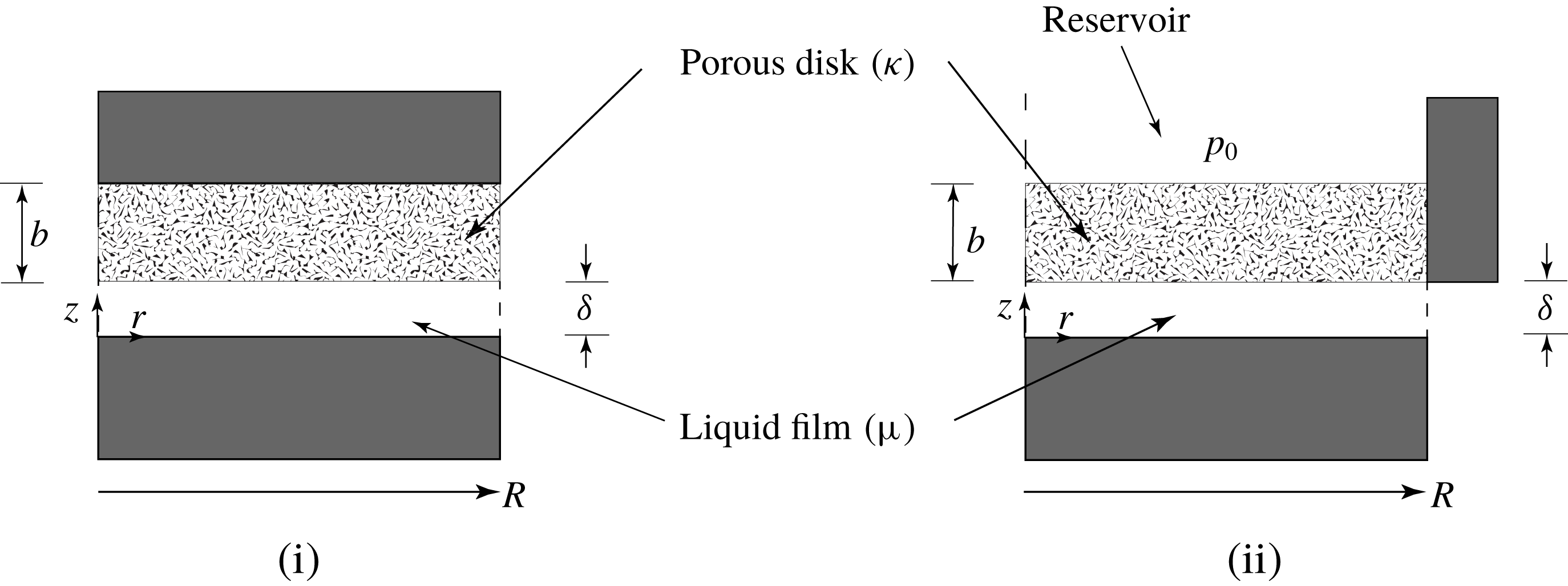
Squeezing flow of liquid film between porous and impermeable disks. The porous disk has permeability
 $\unicode[STIX]{x1D705}$
, thickness
 $b$
and radius
 $R$
(
 $\unicode[STIX]{x1D700}=b/R$
). For the ‘sealed-face’ configuration (i) the upper surface of the porous disk is impermeable; for the ‘sealed-edge’ configuration (ii) the upper surface of the porous disk is permeable and in contact with a reservoir having uniform pressure
 $p_{0}$
.

Squeeze flows of liquid films are encountered in numerous applications. The most obvious of these include lubrication in thrust bearings (Hamrock, Schmid & Jacobson Reference Hamrock, Schmid and Jacobson2004). Other interesting applications include joint lubrication (e.g. knees and hips), compression moulding of plastics, adhesion, food texture and consumer products. Squeezing flows have also been used to study the rheological behaviour of complex (non-Newtonian) fluids (Engmann, Servais & Burbidge Reference Engmann, Servais and Burbidge2005) and soft solids (Meteen Reference Meteen2002; Coussot Reference Coussot2014), which are relevant to many of the applications just mentioned. The dynamics of squeezing liquid films is also important in a rheological technique known as lubricated squeezing flow (Chatraei, Macosko & Winter Reference Chatraei, Macosko and Winter1981), which is used to generate equibiaxial elongation deformations in complex fluids. It has been shown that, due to uncontrolled thinning of the low-viscosity liquid films between the sample and the solid disks, lubricated squeezing flow is limited to relatively small strains (Kompani & Venerus Reference Kompani and Venerus2000; Venerus, Kompani & Bernstein Reference Venerus, Kompani and Bernstein2000; Guadarrama-Medina, Shiu & Venerus Reference Guadarrama-Medina, Shiu and Venerus2009).
Squeezing flows between a solid disk and a porous disk have been investigated because of their relevance to thrust bearings and to the load-bearing characteristics of diathrodial (e.g. knee and hip) joints (Hou et al.
Reference Hou, Mow, Lai and Holmes1992; Ateshian Reference Ateshian2009). The geometry of interest is shown in figure 1 where a liquid film of thickness
 $\unicode[STIX]{x1D6FF}$
is squeezed between disks of radius
 $R$
. The lower disk is impermeable while the upper disk with thickness
 $b$
is porous and has uniform permeability
 $\unicode[STIX]{x1D705}$
. In the ‘sealed-face’ configuration (i), the upper surface of the porous disk is impermeable and the cylindrical external surface is permeable and exposed to ambient pressure. In the ‘sealed-edge’ configuration (ii), the cylindrical external surface of the porous disk is impermeable and its upper surface is permeable and in contact with a reservoir having uniform pressure
 $p_{0}$
. If
 $p_{0}$
is greater than ambient pressure, liquid flows from the porous disk into the liquid film and configuration (ii) is then referred to as an ‘externally pressurized bearing’.
Typically, the equations governing squeezing flows bound by a porous surface are based on Darcy’s law to describe flow in the porous medium and the lubrication approximation to describe flow in the liquid film. The latter governs the liquid film pressure, which is a boundary condition for the equation governing the pressure in the porous disk. Hence, the system of equations is coupled. Whereas the no-slip condition is frequently used to describe squeeze flows between impermeable surfaces, a slip velocity is believed to be necessary to formulate boundary conditions at permeable surfaces (Beavers & Joseph Reference Beavers and Joseph1967), which further couples the governing equations. It is also worth noting for squeezing flows with porous disks that if a constant force is exerted on one of the disks, then the distance between the disks vanishes for finite times.
The first studies of squeezing flow involving a porous surface considered the sealed-face configuration (i) and use Darcy’s law to describe flow in the porous disk. In these studies, squeeze flows show a load-bearing capacity, which depends on the dimensionless parameters
 $\unicode[STIX]{x1D6F9}=\unicode[STIX]{x1D705}b/\unicode[STIX]{x1D6FF}^{3}$
and
 $\unicode[STIX]{x1D700}=b/R$
, that is reduced compared to that of impermeable disks. Wu (Reference Wu1970) and Sparrow, Beavers & Huang (Reference Sparrow, Beavers and Huang1972) found analytical solutions for the case of a porous annular disk without and with, respectively, a slip velocity. An analytical solution for the case of a porous circular disk without a slip velocity was reported shortly thereafter (Murti Reference Murti1974b
). Approximate solutions that include a slip velocity have also been found for annular, circular, rectangular and elliptical porous surfaces (Prakash & Vij Reference Prakash and Vij1974). Analytical solutions for rectangular and circular disks with anisotropic permeability have also been reported (Elsharkawy & Nassar Reference Elsharkawy and Nassar1996). More recently, a perturbation solution valid for small
 $\unicode[STIX]{x1D700}$
for squeezing flow with a porous circular disk has been reported (Knox et al.
Reference Knox, Wilson, Duffy and McKee2015). The same approach has been employed to study the effects of a non-uniform liquid film (Knox et al.
Reference Knox, Duffy, McKee and Wilson2017) and a porous disk with anisotropic permeability (Karmakar & Sekhar Reference Karmakar and Sekhar2018). Finally, we note that the effects of fluid viscoelasticity and the elasticity of the porous disk have been considered (Yousefi, Bou-Saïd & Tichy Reference Yousefi, Bou-Saïd and Tichy2015).
A number of studies of squeezing flow involving a porous surface having configuration (i) have used the so-called Brinkman correction to Darcy’s law to describe flow in the porous disk (Lin Reference Lin1996; Lin, Lu & Yang Reference Lin, Lu and Yang2001; Nabhani, Khlifi & Bou-Saïd Reference Nabhani, Khlifi and Bou-Saïd2010). While this approach may be more general, it introduces additional parameters that are not easily determined. We further note that the Brinkman correction is negligible when the disk porosity is large compared with
 $\unicode[STIX]{x1D705}/b^{2}$
(Whitaker Reference Whitaker1999).
Squeeze film flows having the sealed-edge configuration (ii) are less well studied. The externally pressurized version of configuration (ii), in contrast to configuration (i), allows the film thickness to be controlled while supporting a given force by supplying liquid to the porous disk from the reservoir. Murti (Reference Murti1974a
) and Verma (Reference Verma1980) analysed externally pressurized circular bearings with a slip velocity. Approximate analytical solutions were obtained in these studies by assuming that the pressure within the porous disk was a linear function of
 $z$
, that is, the
 $z$
-direction pressure gradient was assumed to be independent of
 $z$
. The validity of this approximation has not been investigated (Murti Reference Murti1974a
; Verma Reference Verma1980), but one would expect it to hold for a thin porous disk (
 $\unicode[STIX]{x1D700}\ll 1$
). A novel modification of the lubricated squeezing flow technique, which addresses the uncontrolled liquid-film thinning issue (Venerus et al.
Reference Venerus, Shiu, Kashyap and Hosttetler2010), is based on using a porous disk with configuration (ii). Recently, this technique has been used to investigate the rheological behaviour of polymer melts in equibiaxial elongation deformations (Mick, Shiu & Venerus Reference Mick, Shiu and Venerus2015; Mick & Venerus Reference Mick and Venerus2017).
In the present study, we investigate squeeze flows in liquid films bound by porous disks. Our primary focus is on the sealed-edge configuration (ii) as only approximate solutions with restricted validity for this case have been reported in the literature. However, since only an approximate solution for porous circular disks with a slip velocity for the sealed-face configuration (i) has been reported, we also present a solution for this case. This allows us to make direct comparisons of the two configurations. In the following section we derive the governing equations for flow in the liquid film and the porous disk and present their solutions for both configurations. This is followed by a presentation and discussion of results where we examine both the flow behaviour in the liquid film and in the porous medium, and investigate the load-bearing characteristics as a function of the porous disk geometry and its permeability. We conclude by summarizing the results of this study.
2 Problem formulation and solution
We consider the squeezing flow of an incompressible Newtonian fluid with constant density
 $\unicode[STIX]{x1D70C}$
and viscosity
 $\unicode[STIX]{x1D707}$
in a film of thickness
 $\unicode[STIX]{x1D6FF}=\unicode[STIX]{x1D6FF}(t)$
between two disks of radius
 $R$
(see figure 1). The lower disk is stationary and impermeable; the origin of the coordinate system is fixed to its upper surface. The upper disk with thickness
 $b$
is porous and has uniform permeability
 $\unicode[STIX]{x1D705}$
. We assume that flow in the porous disk is governed by Darcy’s law and, since
 $\unicode[STIX]{x1D6FF}\ll R$
, that the lubrication approximation holds in the liquid film. There is symmetry about the
 $z$
-axis and we assume the flow is quasi-stationary. Both gravity and inertia are neglected.
2.1 General problem
The velocity in the liquid film is constrained by
 $$\begin{eqnarray}\frac{1}{r}\frac{\unicode[STIX]{x2202}}{\unicode[STIX]{x2202}r}(rv_{r})+\frac{\unicode[STIX]{x2202}v_{z}}{\unicode[STIX]{x2202}z}=0.\end{eqnarray}$$
Invoking the lubrication approximation, i.e. neglecting terms
 ${\sim}(\unicode[STIX]{x1D6FF}/R)^{2}$
and smaller, the
 $r$
-component of the Navier–Stokes equation takes the form
 $$\begin{eqnarray}\unicode[STIX]{x1D707}\frac{\unicode[STIX]{x2202}^{2}v_{r}}{\unicode[STIX]{x2202}z^{2}}=\frac{\text{d}p}{\text{d}r},\end{eqnarray}$$
where we have
 $p=p(r)$
. Boundary conditions at the impermeable disk are given by
 $$\begin{eqnarray}v_{r}(r,0)=0,\quad v_{z}(r,0)=0,\end{eqnarray}$$
and at the permeable disk by
 $$\begin{eqnarray}v_{r}(r,\unicode[STIX]{x1D6FF})=\langle v_{r}\rangle _{s}(r,\unicode[STIX]{x1D6FF})-\frac{\sqrt{\unicode[STIX]{x1D705}}}{\unicode[STIX]{x1D6FC}}\frac{\unicode[STIX]{x2202}v_{r}}{\unicode[STIX]{x2202}z}(r,\unicode[STIX]{x1D6FF}),\quad v_{z}(r,\unicode[STIX]{x1D6FF})=\langle v_{z}\rangle _{s}(r,\unicode[STIX]{x1D6FF})+\dot{\unicode[STIX]{x1D6FF}},\end{eqnarray}$$
where
 $\langle \boldsymbol{v}\rangle _{s}$
is the superficial average velocity in the porous disk (Whitaker Reference Whitaker1999). The first boundary condition in (2.4), for finite values of the dimensionless parameter
 $\unicode[STIX]{x1D6FC}$
, allows for ‘slip’ between the liquid and porous disk (Beavers & Joseph Reference Beavers and Joseph1967), and in the second boundary condition
 $\dot{\unicode[STIX]{x1D6FF}}=\text{d}\unicode[STIX]{x1D6FF}/\text{d}t$
.
Integration of (2.2) with respect to
 $z$
and applying the boundary conditions in (2.3a
) and (2.4a
) gives
 $$\begin{eqnarray}v_{r}=-\frac{\unicode[STIX]{x1D6FF}^{2}}{2\unicode[STIX]{x1D707}}\frac{\text{d}p}{\text{d}r}\left[\frac{1+2\unicode[STIX]{x1D70E}}{1+\unicode[STIX]{x1D70E}}\frac{z}{\unicode[STIX]{x1D6FF}}-\left(\frac{z}{\unicode[STIX]{x1D6FF}}\right)^{2}\right]+\frac{\langle v_{r}\rangle _{s}(r,\unicode[STIX]{x1D6FF})}{1+\unicode[STIX]{x1D70E}}\frac{z}{\unicode[STIX]{x1D6FF}},\end{eqnarray}$$
where
 $\unicode[STIX]{x1D70E}=\sqrt{\unicode[STIX]{x1D705}}/\unicode[STIX]{x1D6FC}\unicode[STIX]{x1D6FF}$
. Substitution of (2.5) in (2.1) gives
 $$\begin{eqnarray}\frac{\unicode[STIX]{x2202}v_{z}}{\unicode[STIX]{x2202}z}=\frac{\unicode[STIX]{x1D6FF}^{2}}{2\unicode[STIX]{x1D707}}\frac{1}{r}\frac{\text{d}}{\text{d}r}\left(r\frac{\text{d}p}{\text{d}r}\right)\left[\frac{1+2\unicode[STIX]{x1D70E}}{1+\unicode[STIX]{x1D70E}}\frac{z}{\unicode[STIX]{x1D6FF}}-\left(\frac{z}{\unicode[STIX]{x1D6FF}}\right)^{2}\right]-\frac{1}{1+\unicode[STIX]{x1D70E}}\frac{1}{r}\frac{\unicode[STIX]{x2202}}{\unicode[STIX]{x2202}r}\left(r\langle v_{r}\rangle _{s}(r,\unicode[STIX]{x1D6FF})\right)\frac{z}{\unicode[STIX]{x1D6FF}}.\end{eqnarray}$$
Integration of (2.6) over
 $z$
from
 $0$
to
 $\unicode[STIX]{x1D6FF}$
with the boundary conditions in (2.3b
) and (2.4b
) gives
 $$\begin{eqnarray}\frac{1}{r}\frac{\text{d}}{\text{d}r}\left(r\frac{\text{d}p}{\text{d}r}\right)=12\frac{1+\unicode[STIX]{x1D70E}}{1+4\unicode[STIX]{x1D70E}}\frac{\unicode[STIX]{x1D707}}{\unicode[STIX]{x1D6FF}^{3}}[\dot{\unicode[STIX]{x1D6FF}}+\langle v_{z}\rangle _{s}(r,\unicode[STIX]{x1D6FF})]+\frac{6}{1+4\unicode[STIX]{x1D70E}}\frac{\unicode[STIX]{x1D707}}{\unicode[STIX]{x1D6FF}^{2}}\frac{1}{r}\frac{\unicode[STIX]{x2202}}{\unicode[STIX]{x2202}r}(r\langle v_{r}\rangle _{s}(r,\unicode[STIX]{x1D6FF})),\end{eqnarray}$$
which is the Reynolds equation for the liquid film. We note that the stress from (2.6) is
 $(\unicode[STIX]{x1D6FF}/R)^{2}$
times smaller than the stress from (2.7).
The superficial average velocity
 $\langle \boldsymbol{v}\rangle _{s}$
in the porous disk is constrained by
 $$\begin{eqnarray}\frac{1}{r}\frac{\unicode[STIX]{x2202}}{\unicode[STIX]{x2202}r}(r\langle v_{r}\rangle _{s})+\frac{\unicode[STIX]{x2202}\langle v_{z}\rangle _{s}}{\unicode[STIX]{x2202}z}=0.\end{eqnarray}$$
The superficial average streamfunction
 $\langle \unicode[STIX]{x1D713}\rangle _{s}$
is defined by the relations
 $$\begin{eqnarray}\langle v_{r}\rangle _{s}=-\frac{1}{r}\frac{\unicode[STIX]{x2202}\langle \unicode[STIX]{x1D713}\rangle _{s}}{\unicode[STIX]{x2202}z},\quad \langle v_{z}\rangle _{s}=\frac{1}{r}\frac{\unicode[STIX]{x2202}\langle \unicode[STIX]{x1D713}\rangle _{s}}{\unicode[STIX]{x2202}r}.\end{eqnarray}$$
We assume flow in the porous disk is governed by Darcy’s law, which takes the form
 $$\begin{eqnarray}\langle v_{r}\rangle _{s}=-\frac{\unicode[STIX]{x1D705}}{\unicode[STIX]{x1D707}}\frac{\unicode[STIX]{x2202}\langle p\rangle _{i}}{\unicode[STIX]{x2202}r},\quad \langle v_{z}\rangle _{s}=-\frac{\unicode[STIX]{x1D705}}{\unicode[STIX]{x1D707}}\frac{\unicode[STIX]{x2202}\langle p\rangle _{i}}{\unicode[STIX]{x2202}z},\end{eqnarray}$$
where
 $\langle p\rangle _{i}$
is the intrinsic average pressure within the porous disk (Whitaker Reference Whitaker1999). Combining (2.8) and (2.10), we have
 $$\begin{eqnarray}\frac{1}{r}\frac{\unicode[STIX]{x2202}}{\unicode[STIX]{x2202}r}\left(r\frac{\unicode[STIX]{x2202}\langle p\rangle _{i}}{\unicode[STIX]{x2202}r}\right)+\frac{\unicode[STIX]{x2202}^{2}\langle p\rangle _{i}}{\unicode[STIX]{x2202}z^{2}}=0,\end{eqnarray}$$
which is solved subject to
 $\unicode[STIX]{x2202}\langle p\rangle _{i}/\unicode[STIX]{x2202}r(0,z)=0$
and the boundary condition
 $$\begin{eqnarray}\langle p\rangle _{i}(r,\unicode[STIX]{x1D6FF})=p(r).\end{eqnarray}$$
Using (2.10) and (2.11), we can write (2.7) as
 $$\begin{eqnarray}\frac{1}{r}\frac{\text{d}}{\text{d}r}\left(r\frac{\text{d}p}{\text{d}r}\right)=12\frac{1+\unicode[STIX]{x1D70E}}{1+4\unicode[STIX]{x1D70E}}\frac{\unicode[STIX]{x1D707}\dot{\unicode[STIX]{x1D6FF}}}{\unicode[STIX]{x1D6FF}^{3}}-12\frac{1+\unicode[STIX]{x1D70E}}{1+4\unicode[STIX]{x1D70E}}\frac{\unicode[STIX]{x1D705}}{\unicode[STIX]{x1D6FF}^{3}}\frac{\unicode[STIX]{x2202}\langle p\rangle _{i}}{\unicode[STIX]{x2202}z}(r,\unicode[STIX]{x1D6FF})+\frac{6}{1+4\unicode[STIX]{x1D70E}}\frac{\unicode[STIX]{x1D705}}{\unicode[STIX]{x1D6FF}^{2}}\frac{\unicode[STIX]{x2202}^{2}\langle p\rangle _{i}}{\unicode[STIX]{x2202}z^{2}}(r,\unicode[STIX]{x1D6FF}),\end{eqnarray}$$
which is solved subject to
 $\text{d}p/\text{d}r(0)=0$
and
 $p(R)=0$
. The coupled system of (2.11)–(2.13) applies to both configurations (i) and (ii). To solve (2.11) for
 $\langle p\rangle _{i}$
, additional boundary conditions must be prescribed.
Finally, the force exerted by the liquid film on the porous disk is obtained from
 $$\begin{eqnarray}{\mathcal{F}}=2\unicode[STIX]{x03C0}\int _{0}^{R}p(r)r\,\text{d}r,\end{eqnarray}$$
where, as noted previously, we are neglecting terms from (2.6) that are
 $(\unicode[STIX]{x1D6FF}/R)^{2}$
times smaller than those being retained.
2.2 Solution for the sealed-face configuration (i)
First, we consider the sealed-face configuration (i) shown in figure 1 for which the boundary conditions for (2.11) are
 $$\begin{eqnarray}\displaystyle & \displaystyle \frac{\unicode[STIX]{x2202}\langle p\rangle _{i}}{\unicode[STIX]{x2202}z}(r,\unicode[STIX]{x1D6FF}+b)=0, & \displaystyle\end{eqnarray}$$
 $$\begin{eqnarray}\displaystyle & \displaystyle \langle p\rangle _{i}(R,z)=0. & \displaystyle\end{eqnarray}$$
The solution to (2.11) subject to (2.12), (2.15) and (2.16) can be written as
 $$\begin{eqnarray}\langle p\rangle _{i}=\mathop{\sum }_{n=1}^{\infty }B_{n}\frac{\text{J}_{0}(\unicode[STIX]{x1D6FD}_{n}r)\cosh [\unicode[STIX]{x1D6FD}_{n}(\unicode[STIX]{x1D6FF}+b-z)]}{\cosh (\unicode[STIX]{x1D6FD}_{n}b)},\end{eqnarray}$$
where
 $\text{J}_{0}(x)$
is the Bessel function of the first kind. The
 $\unicode[STIX]{x1D6FD}_{n}$
are found from the roots of
 $\text{J}_{0}(\unicode[STIX]{x1D6FD}_{n}R)=0,n=1,2,3,\ldots \,$
, and
 $$\begin{eqnarray}B_{n}=\frac{2}{R^{2}\text{J}_{1}^{2}(\unicode[STIX]{x1D6FD}_{n}R)}\int _{0}^{R}p(r)\text{J}_{0}(\unicode[STIX]{x1D6FD}_{n}r)r\,\text{d}r,\quad n=1,2,3,\ldots .\end{eqnarray}$$
Substituting (2.17) in (2.13), we obtain
 $$\begin{eqnarray}\frac{1}{r}\frac{\text{d}}{\text{d}r}\left(r\frac{\text{d}p}{\text{d}r}\right)=12\frac{1+\unicode[STIX]{x1D70E}}{1+4\unicode[STIX]{x1D70E}}\frac{\unicode[STIX]{x1D707}\dot{\unicode[STIX]{x1D6FF}}}{\unicode[STIX]{x1D6FF}^{3}}+\frac{12}{1+4\unicode[STIX]{x1D70E}}\frac{\unicode[STIX]{x1D705}}{\unicode[STIX]{x1D6FF}^{3}}\mathop{\sum }_{n=1}^{\infty }B_{n}\left[(1+\unicode[STIX]{x1D70E})\tanh (\unicode[STIX]{x1D6FD}_{n}b)+\frac{1}{2}\unicode[STIX]{x1D6FF}\unicode[STIX]{x1D6FD}_{n}\right]\unicode[STIX]{x1D6FD}_{n}\text{J}_{0}(\unicode[STIX]{x1D6FD}_{n}r).\end{eqnarray}$$
Integrating (2.19) twice with respect to
 $r$
gives
 $$\begin{eqnarray}p=-3\frac{1+\unicode[STIX]{x1D70E}}{1+4\unicode[STIX]{x1D70E}}\unicode[STIX]{x1D707}\frac{R^{2}}{\unicode[STIX]{x1D6FF}^{3}}\dot{\unicode[STIX]{x1D6FF}}\!\left[1-\left(\frac{r}{R}\right)^{2}\right]-\frac{12}{1+4\unicode[STIX]{x1D70E}}\frac{\unicode[STIX]{x1D705}R}{\unicode[STIX]{x1D6FF}^{3}}\mathop{\sum }_{n=1}^{\infty }B_{n}\!\left[(1+\unicode[STIX]{x1D70E})\frac{\tanh (\unicode[STIX]{x1D6FD}_{n}b)}{\unicode[STIX]{x1D6FD}_{n}R}+\frac{1}{2}\frac{\unicode[STIX]{x1D6FF}}{R}\right]\!\text{J}_{0}(\unicode[STIX]{x1D6FD}_{n}r).\end{eqnarray}$$
Substitution of (2.20) in (2.18) gives
 $$\begin{eqnarray}B_{n}=-24\frac{1+\unicode[STIX]{x1D70E}}{1+4\unicode[STIX]{x1D70E}}\unicode[STIX]{x1D707}\dot{\unicode[STIX]{x1D6FF}}\frac{R^{2}}{\unicode[STIX]{x1D6FF}^{3}}\frac{1}{(\unicode[STIX]{x1D6FD}_{n}R)^{3}\text{J}_{1}(\unicode[STIX]{x1D6FD}_{n}R)}\left\{1+\frac{12}{1+4\unicode[STIX]{x1D70E}}\frac{\unicode[STIX]{x1D705}R}{\unicode[STIX]{x1D6FF}^{3}}\left[(1+\unicode[STIX]{x1D70E})\frac{\tanh (\unicode[STIX]{x1D6FD}_{n}b)}{\unicode[STIX]{x1D6FD}_{n}R}+\frac{1}{2}\frac{\unicode[STIX]{x1D6FF}}{R}\right]\right\}^{-1}.\end{eqnarray}$$
Substituting (2.21) in (2.20) we obtain
 $$\begin{eqnarray}\frac{p\unicode[STIX]{x1D6FF}^{3}}{\unicode[STIX]{x1D707}R^{2}}=-3\frac{1+\unicode[STIX]{x1D70E}}{1+4\unicode[STIX]{x1D70E}}\dot{\unicode[STIX]{x1D6FF}}\mathop{\sum }_{n=1}^{\infty }\frac{8}{\bar{\unicode[STIX]{x1D6FD}}_{n}^{3}}\left\{1+\frac{12\unicode[STIX]{x1D6F6}}{1+4\unicode[STIX]{x1D70E}}\left[(1+\unicode[STIX]{x1D70E})\frac{\tanh (\bar{\unicode[STIX]{x1D6FD}}_{n}\unicode[STIX]{x1D700})}{\bar{\unicode[STIX]{x1D6FD}}_{n}}+\frac{1}{2}\frac{\unicode[STIX]{x1D6FF}}{R}\right]\right\}^{-1}\frac{\text{J}_{0}(\bar{\unicode[STIX]{x1D6FD}}_{n}r/R)}{\text{J}_{1}(\bar{\unicode[STIX]{x1D6FD}}_{n})},\end{eqnarray}$$
where
 $\bar{\unicode[STIX]{x1D6FD}}_{n}=\unicode[STIX]{x1D6FD}_{n}R$
,
 $\unicode[STIX]{x1D700}=b/R$
and
 $\unicode[STIX]{x1D6F6}=\unicode[STIX]{x1D705}R/\unicode[STIX]{x1D6FF}^{3}$
(note that
 $\unicode[STIX]{x1D6F6}=\unicode[STIX]{x1D6F9}/\unicode[STIX]{x1D700}$
). Substituting (2.21) in (2.17) we obtain
 $$\begin{eqnarray}\displaystyle \frac{\langle p\rangle _{i}\unicode[STIX]{x1D6FF}^{3}}{\unicode[STIX]{x1D707}R^{2}} & = & \displaystyle -3\frac{1+\unicode[STIX]{x1D70E}}{1+4\unicode[STIX]{x1D70E}}\dot{\unicode[STIX]{x1D6FF}}\mathop{\sum }_{n=1}^{\infty }\frac{8}{\bar{\unicode[STIX]{x1D6FD}}_{n}^{3}}\left\{1+\frac{12\unicode[STIX]{x1D6F6}}{1+4\unicode[STIX]{x1D70E}}\left[(1+\unicode[STIX]{x1D70E})\frac{\tanh (\bar{\unicode[STIX]{x1D6FD}}_{n}\unicode[STIX]{x1D700})}{\bar{\unicode[STIX]{x1D6FD}}_{n}}+\frac{1}{2}\frac{\unicode[STIX]{x1D6FF}}{R}\right]\right\}^{-1}\nonumber\\ \displaystyle & & \displaystyle \times \,\frac{\text{J}_{0}(\bar{\unicode[STIX]{x1D6FD}}_{n}r/R)\cosh \left(\bar{\unicode[STIX]{x1D6FD}}_{n}\unicode[STIX]{x1D700}[1-(z-\unicode[STIX]{x1D6FF})/b]\right)}{\text{J}_{1}(\bar{\unicode[STIX]{x1D6FD}}_{n})\cosh (\bar{\unicode[STIX]{x1D6FD}}_{n}\unicode[STIX]{x1D700})},\end{eqnarray}$$
and from (2.5) using (2.22) and (2.23), we find
 $$\begin{eqnarray}\displaystyle \frac{v_{r}\unicode[STIX]{x1D6FF}}{R} & = & \displaystyle -\frac{12}{1+4\unicode[STIX]{x1D70E}}\dot{\unicode[STIX]{x1D6FF}}\left[\left(1+2\unicode[STIX]{x1D70E}+2\frac{\unicode[STIX]{x1D6FF}}{R}\unicode[STIX]{x1D6F6}\right)\frac{z}{\unicode[STIX]{x1D6FF}}-(1+\unicode[STIX]{x1D70E})\left(\frac{z}{\unicode[STIX]{x1D6FF}}\right)^{2}\right]\nonumber\\ \displaystyle & & \displaystyle \times \,\mathop{\sum }_{n=1}^{\infty }\left\{1+\frac{12\unicode[STIX]{x1D6F6}}{1+4\unicode[STIX]{x1D70E}}\left[(1+\unicode[STIX]{x1D70E})\frac{\tanh (\bar{\unicode[STIX]{x1D6FD}}_{n}\unicode[STIX]{x1D700})}{\bar{\unicode[STIX]{x1D6FD}}_{n}}+\frac{1}{2}\frac{\unicode[STIX]{x1D6FF}}{R}\right]\right\}^{-1}\frac{\text{J}_{1}(\bar{\unicode[STIX]{x1D6FD}}_{n}r/R)}{\bar{\unicode[STIX]{x1D6FD}}_{n}^{2}\text{J}_{1}(\bar{\unicode[STIX]{x1D6FD}}_{n})}.\end{eqnarray}$$
Using (2.23) with (2.10) and (2.9) we obtain
 $$\begin{eqnarray}\displaystyle \frac{\langle \unicode[STIX]{x1D713}\rangle _{s}}{R^{2}} & = & \displaystyle -3\dot{\unicode[STIX]{x1D6FF}}\frac{1+\unicode[STIX]{x1D70E}}{1+4\unicode[STIX]{x1D70E}}\unicode[STIX]{x1D6F6}\mathop{\sum }_{n=1}^{\infty }\frac{8}{\bar{\unicode[STIX]{x1D6FD}}_{n}^{3}}\left\{1+\frac{12\unicode[STIX]{x1D6F6}}{1+4\unicode[STIX]{x1D70E}}\left[(1+\unicode[STIX]{x1D70E})\frac{\tanh (\bar{\unicode[STIX]{x1D6FD}}_{n}\unicode[STIX]{x1D700})}{\bar{\unicode[STIX]{x1D6FD}}_{n}}+\frac{1}{2}\frac{\unicode[STIX]{x1D6FF}}{R}\right]\right\}^{-1}\nonumber\\ \displaystyle & & \displaystyle \times \,\frac{(r/R)\text{J}_{1}(\bar{\unicode[STIX]{x1D6FD}}_{n}r/R)\sinh \left(\bar{\unicode[STIX]{x1D6FD}}_{n}\unicode[STIX]{x1D700}[1-(z-\unicode[STIX]{x1D6FF})/b]\right)}{\text{J}_{1}(\bar{\unicode[STIX]{x1D6FD}}_{n})\cosh (\bar{\unicode[STIX]{x1D6FD}}_{n}\unicode[STIX]{x1D700})}.\end{eqnarray}$$
Finally, substituting (2.22) in (2.14) we obtain
 $$\begin{eqnarray}\frac{2{\mathcal{F}}}{3\unicode[STIX]{x1D707}\unicode[STIX]{x03C0}R^{4}}=-\frac{1+\unicode[STIX]{x1D70E}}{1+4\unicode[STIX]{x1D70E}}\frac{\dot{\unicode[STIX]{x1D6FF}}}{\unicode[STIX]{x1D6FF}^{3}}\mathop{\sum }_{n=1}^{\infty }\frac{32}{\bar{\unicode[STIX]{x1D6FD}}_{n}^{4}}\left\{1+\frac{12\unicode[STIX]{x1D6F6}}{1+4\unicode[STIX]{x1D70E}}\left[(1+\unicode[STIX]{x1D70E})\frac{\tanh (\bar{\unicode[STIX]{x1D6FD}}_{n}\unicode[STIX]{x1D700})}{\bar{\unicode[STIX]{x1D6FD}}_{n}}+\frac{1}{2}\frac{\unicode[STIX]{x1D6FF}}{R}\right]\right\}^{-1},\end{eqnarray}$$
(note that
 $\sum _{n=1}^{\infty }32/\bar{\unicode[STIX]{x1D6FD}}_{n}^{4}=1$
). For the no-slip case (
 $\unicode[STIX]{x1D70E}=0$
), the expressions in (2.22) and (2.26) simplify to those given by Murti (Reference Murti1974b
).
2.3 Solution for the sealed-edge configuration (ii)
For the sealed-edge configuration (ii) shown in figure 1, we have the boundary conditions
 $$\begin{eqnarray}\displaystyle & \displaystyle \langle p\rangle _{i}(r,\unicode[STIX]{x1D6FF}+b)=p_{0}, & \displaystyle\end{eqnarray}$$
 $$\begin{eqnarray}\displaystyle & \displaystyle \frac{\unicode[STIX]{x2202}\langle p\rangle _{i}}{\unicode[STIX]{x2202}r}(R,z)=0. & \displaystyle\end{eqnarray}$$
The solution of (2.11) subject to (2.12), (2.27) and (2.28) can be written as
 $$\begin{eqnarray}\langle p\rangle _{i}=p_{0}+(p_{0}-\bar{p})\left(\frac{z-\unicode[STIX]{x1D6FF}}{b}-1\right)+\mathop{\sum }_{n=1}^{\infty }A_{n}\frac{\text{J}_{0}(\unicode[STIX]{x1D6FC}_{n}r)\sinh [\unicode[STIX]{x1D6FC}_{n}(\unicode[STIX]{x1D6FF}+b-z)]}{\sinh [\unicode[STIX]{x1D6FC}_{n}b]},\end{eqnarray}$$
where
 $$\begin{eqnarray}\bar{p}=\frac{2}{R^{2}}\int _{0}^{R}p(r)r\,\text{d}r\end{eqnarray}$$
is the average pressure in the liquid film. The
 $\unicode[STIX]{x1D6FC}_{n}$
are found from the roots of
 $\text{J}_{1}(\unicode[STIX]{x1D6FC}_{n}R)=0,n=0,1,2,\ldots \,$
, which includes
 $\unicode[STIX]{x1D6FC}_{0}=0$
, and the
 $A_{n}$
are given by
 $$\begin{eqnarray}A_{n}=\frac{2}{R^{2}\text{J}_{0}^{2}(\unicode[STIX]{x1D6FC}_{n}R)}\int _{0}^{R}p(r)\text{J}_{0}(\unicode[STIX]{x1D6FC}_{n}r)r\,\text{d}r,\quad n=1,2,3,\ldots .\end{eqnarray}$$
The total mass flow rate
 ${\mathcal{W}}$
from the reservoir to the porous disk is given by
 $$\begin{eqnarray}\frac{{\mathcal{W}}}{\unicode[STIX]{x1D70C}\unicode[STIX]{x03C0}}=-2\int _{0}^{R}\langle v_{z}\rangle _{s}(r,b+\unicode[STIX]{x1D6FF})r\,\text{d}r=\frac{\unicode[STIX]{x1D705}R^{2}}{\unicode[STIX]{x1D707}b}(p_{0}-\bar{p}),\end{eqnarray}$$
where the second equality is obtained using (2.10b ) and (2.29).
Substitution of (2.29) in (2.13) leads to
 $$\begin{eqnarray}\displaystyle \frac{1}{r}\frac{\text{d}}{\text{d}r}\left(r\frac{\text{d}p}{\text{d}r}\right) & = & \displaystyle 12\frac{1+\unicode[STIX]{x1D70E}}{1+4\unicode[STIX]{x1D70E}}\frac{\unicode[STIX]{x1D707}}{\unicode[STIX]{x1D6FF}^{3}}\left[\dot{\unicode[STIX]{x1D6FF}}-\frac{\unicode[STIX]{x1D705}}{\unicode[STIX]{x1D707}b}(p_{0}-\bar{p})\right]\nonumber\\ \displaystyle & & \displaystyle -\,\frac{12}{1+4\unicode[STIX]{x1D70E}}\frac{\unicode[STIX]{x1D705}}{\unicode[STIX]{x1D6FF}^{3}}\mathop{\sum }_{n=1}^{\infty }A_{n}\left[(1+\unicode[STIX]{x1D70E})\coth (\unicode[STIX]{x1D6FC}_{n}b)+\frac{1}{2}\unicode[STIX]{x1D6FF}\unicode[STIX]{x1D6FC}_{n}\right]\unicode[STIX]{x1D6FC}_{n}\text{J}_{0}(\unicode[STIX]{x1D6FC}_{n}r).\qquad\end{eqnarray}$$
Integrating (2.33) twice with respect to
 $r$
gives
 $$\begin{eqnarray}\displaystyle p & = & \displaystyle -3\frac{1+\unicode[STIX]{x1D70E}}{1+4\unicode[STIX]{x1D70E}}\unicode[STIX]{x1D707}\frac{R^{2}}{\unicode[STIX]{x1D6FF}^{3}}\left[\dot{\unicode[STIX]{x1D6FF}}-\frac{\unicode[STIX]{x1D705}}{\unicode[STIX]{x1D707}b}(p_{0}-\bar{p})\right]\left[1-\left(\frac{r}{R}\right)^{2}\right]\nonumber\\ \displaystyle & & \displaystyle +\,\frac{12}{1+4\unicode[STIX]{x1D70E}}\frac{\unicode[STIX]{x1D705}R}{\unicode[STIX]{x1D6FF}^{3}}\mathop{\sum }_{n=1}^{\infty }A_{n}\left[(1+\unicode[STIX]{x1D70E})\frac{\coth (\unicode[STIX]{x1D6FC}_{n}b)}{\unicode[STIX]{x1D6FC}_{n}R}+\frac{1}{2}\frac{\unicode[STIX]{x1D6FF}}{R}\right][\text{J}_{0}(\unicode[STIX]{x1D6FC}_{n}R)-\text{J}_{0}(\unicode[STIX]{x1D6FC}_{n}r)].\qquad\end{eqnarray}$$
Substitution of (2.34) in (2.31) gives
 $$\begin{eqnarray}\displaystyle A_{n} & = & \displaystyle 12\frac{1+\unicode[STIX]{x1D70E}}{1+4\unicode[STIX]{x1D70E}}\unicode[STIX]{x1D707}\frac{R^{2}}{\unicode[STIX]{x1D6FF}^{3}}\left(\dot{\unicode[STIX]{x1D6FF}}-\frac{{\mathcal{W}}}{\unicode[STIX]{x1D70C}\unicode[STIX]{x03C0}R^{2}}\right)\frac{1}{(\unicode[STIX]{x1D6FC}_{n}R)^{2}\text{J}_{0}(\unicode[STIX]{x1D6FC}_{n}R)}\nonumber\\ \displaystyle & & \displaystyle \times \,\left\{1+\frac{12}{1+4\unicode[STIX]{x1D70E}}\frac{\unicode[STIX]{x1D705}R}{\unicode[STIX]{x1D6FF}^{3}}\left[(1+\unicode[STIX]{x1D70E})\frac{\coth (\unicode[STIX]{x1D6FC}_{n}b)}{\unicode[STIX]{x1D6FC}_{n}R}+\frac{1}{2}\frac{\unicode[STIX]{x1D6FF}}{R}\right]\right\}^{-1},\end{eqnarray}$$
where (2.32) has been used. Using (2.34) and (2.35), the pressure in the liquid film is given by
 $$\begin{eqnarray}\displaystyle \frac{p\unicode[STIX]{x1D6FF}^{3}}{\unicode[STIX]{x1D707}R^{2}} & = & \displaystyle -3\frac{1+\unicode[STIX]{x1D70E}}{1+4\unicode[STIX]{x1D70E}}\left(\dot{\unicode[STIX]{x1D6FF}}-\frac{{\mathcal{W}}}{\unicode[STIX]{x1D70C}\unicode[STIX]{x03C0}R^{2}}\right)\mathop{\sum }_{n=1}^{\infty }\frac{4}{\bar{\unicode[STIX]{x1D6FC}}_{n}^{2}}\left\{1+\frac{12\unicode[STIX]{x1D6F6}}{1+4\unicode[STIX]{x1D70E}}\left[(1+\unicode[STIX]{x1D70E})\frac{\coth (\bar{\unicode[STIX]{x1D6FC}}_{n}\unicode[STIX]{x1D700})}{\bar{\unicode[STIX]{x1D6FC}}_{n}}+\frac{1}{2}\frac{\unicode[STIX]{x1D6FF}}{R}\right]\right\}^{-1}\nonumber\\ \displaystyle & & \displaystyle \times \,\left[1-\frac{\text{J}_{0}(\bar{\unicode[STIX]{x1D6FC}}_{n}r/R)}{\text{J}_{0}(\bar{\unicode[STIX]{x1D6FC}}_{n})}\right],\end{eqnarray}$$
where
 $\bar{\unicode[STIX]{x1D6FC}}_{n}=\unicode[STIX]{x1D6FC}_{n}R$
. Combining (2.30), (2.32) and (2.36),
 $p_{0}$
is given by
 $$\begin{eqnarray}\displaystyle \frac{p_{0}\unicode[STIX]{x1D6FF}^{3}}{\unicode[STIX]{x1D707}R^{2}} & = & \displaystyle \frac{{\mathcal{W}}}{\unicode[STIX]{x1D70C}\unicode[STIX]{x03C0}R^{2}}\frac{\unicode[STIX]{x1D700}}{\unicode[STIX]{x1D6F6}}-\frac{3}{2}\frac{1+\unicode[STIX]{x1D70E}}{1+4\unicode[STIX]{x1D70E}}\left(\dot{\unicode[STIX]{x1D6FF}}-\frac{{\mathcal{W}}}{\unicode[STIX]{x1D70C}\unicode[STIX]{x03C0}R^{2}}\right)\mathop{\sum }_{n=1}^{\infty }\frac{8}{\bar{\unicode[STIX]{x1D6FC}}_{n}^{2}}\nonumber\\ \displaystyle & & \displaystyle \times \,\left\{1+\frac{12\unicode[STIX]{x1D6F6}}{1+4\unicode[STIX]{x1D70E}}\left[(1+\unicode[STIX]{x1D70E})\frac{\coth (\bar{\unicode[STIX]{x1D6FC}}_{n}\unicode[STIX]{x1D700})}{\bar{\unicode[STIX]{x1D6FC}}_{n}}+\frac{1}{2}\frac{\unicode[STIX]{x1D6FF}}{R}\right]\right\}^{-1}.\end{eqnarray}$$
To obtain
 $\langle p\rangle _{i}$
, (2.32), (2.35) and (2.37) are substituted in (2.29), which gives
 $$\begin{eqnarray}\displaystyle \frac{\langle p\rangle _{i}\unicode[STIX]{x1D6FF}^{3}}{\unicode[STIX]{x1D707}R^{2}} & = & \displaystyle \frac{{\mathcal{W}}}{\unicode[STIX]{x1D70C}\unicode[STIX]{x03C0}R^{2}}\frac{\unicode[STIX]{x1D700}}{\unicode[STIX]{x1D6F6}}\frac{z-\unicode[STIX]{x1D6FF}}{b}-\frac{3}{2}\frac{1+\unicode[STIX]{x1D70E}}{1+4\unicode[STIX]{x1D70E}}\left(\dot{\unicode[STIX]{x1D6FF}}-\frac{{\mathcal{W}}}{\unicode[STIX]{x1D70C}\unicode[STIX]{x03C0}R^{2}}\right)\nonumber\\ \displaystyle & & \displaystyle \times \,\mathop{\sum }_{n=1}^{\infty }\frac{8}{\bar{\unicode[STIX]{x1D6FC}}_{n}^{2}}\left\{1+\frac{12\unicode[STIX]{x1D6F6}}{1+4\unicode[STIX]{x1D70E}}\left[(1+\unicode[STIX]{x1D70E})\frac{\coth (\bar{\unicode[STIX]{x1D6FC}}_{n}\unicode[STIX]{x1D700})}{\bar{\unicode[STIX]{x1D6FC}}_{n}}+\frac{1}{2}\frac{\unicode[STIX]{x1D6FF}}{R}\right]\right\}^{-1}\nonumber\\ \displaystyle & & \displaystyle \times \,\left[1-\frac{\text{J}_{0}(\bar{\unicode[STIX]{x1D6FC}}_{n}r/R)\sinh \left(\bar{\unicode[STIX]{x1D6FC}}_{n}\unicode[STIX]{x1D700}[1-(z-\unicode[STIX]{x1D6FF})/b]\right)}{\text{J}_{0}(\bar{\unicode[STIX]{x1D6FC}}_{n})\sinh (\bar{\unicode[STIX]{x1D6FC}}_{n}\unicode[STIX]{x1D700})}\right].\end{eqnarray}$$
From (2.5) using (2.36) and (2.38), we find
 $$\begin{eqnarray}\displaystyle \frac{v_{r}\unicode[STIX]{x1D6FF}}{R} & = & \displaystyle \frac{6}{1+4\unicode[STIX]{x1D70E}}\left(\dot{\unicode[STIX]{x1D6FF}}-\frac{{\mathcal{W}}}{\unicode[STIX]{x1D70C}\unicode[STIX]{x03C0}R^{2}}\right)\left[\left(1+2\unicode[STIX]{x1D70E}+2\frac{\unicode[STIX]{x1D6FF}}{R}\unicode[STIX]{x1D6F6}\right)\frac{z}{\unicode[STIX]{x1D6FF}}-(1+\unicode[STIX]{x1D70E})\left(\frac{z}{\unicode[STIX]{x1D6FF}}\right)^{2}\right]\nonumber\\ \displaystyle & & \displaystyle \times \,\mathop{\sum }_{n=1}^{\infty }\left\{1+\frac{12\unicode[STIX]{x1D6F6}}{1+4\unicode[STIX]{x1D70E}}\left[(1+\unicode[STIX]{x1D70E})\frac{\coth (\bar{\unicode[STIX]{x1D6FC}}_{n}\unicode[STIX]{x1D700})}{\bar{\unicode[STIX]{x1D6FC}}_{n}}+\frac{1}{2}\frac{\unicode[STIX]{x1D6FF}}{R}\right]\right\}^{-1}\frac{\text{J}_{1}(\bar{\unicode[STIX]{x1D6FC}}_{n}r/R)}{\bar{\unicode[STIX]{x1D6FC}}_{n}\text{J}_{0}(\bar{\unicode[STIX]{x1D6FC}}_{n})}.\end{eqnarray}$$
Using (2.38) with (2.10) and (2.9) we obtain
 $$\begin{eqnarray}\displaystyle \frac{\langle \unicode[STIX]{x1D713}\rangle _{s}}{R^{2}} & = & \displaystyle -\frac{1}{2}\frac{{\mathcal{W}}}{\unicode[STIX]{x1D70C}\unicode[STIX]{x03C0}R^{2}}\left(\frac{r}{R}\right)^{2}+\frac{3}{2}\frac{1+\unicode[STIX]{x1D70E}}{1+4\unicode[STIX]{x1D70E}}\unicode[STIX]{x1D6F6}\left(\dot{\unicode[STIX]{x1D6FF}}-\frac{{\mathcal{W}}}{\unicode[STIX]{x1D70C}\unicode[STIX]{x03C0}R^{2}}\right)\nonumber\\ \displaystyle & & \displaystyle \times \,\mathop{\sum }_{n=1}^{\infty }\frac{8}{\bar{\unicode[STIX]{x1D6FC}}_{n}^{2}}\left\{1+\frac{12\unicode[STIX]{x1D6F6}}{1+4\unicode[STIX]{x1D70E}}\left[(1+\unicode[STIX]{x1D70E})\frac{\tanh (\bar{\unicode[STIX]{x1D6FC}}_{n}\unicode[STIX]{x1D700})}{\bar{\unicode[STIX]{x1D6FC}}_{n}}+\frac{1}{2}\frac{\unicode[STIX]{x1D6FF}}{R}\right]\right\}^{-1}\nonumber\\ \displaystyle & & \displaystyle \times \,\frac{(r/R)\text{J}_{1}(\bar{\unicode[STIX]{x1D6FC}}_{n}r/R)\cosh \left(\bar{\unicode[STIX]{x1D6FC}}_{n}\unicode[STIX]{x1D700}[1-(z-\unicode[STIX]{x1D6FF})/b]\right)}{\text{J}_{0}(\bar{\unicode[STIX]{x1D6FC}}_{n})\sinh (\bar{\unicode[STIX]{x1D6FC}}_{n}\unicode[STIX]{x1D700})}.\end{eqnarray}$$
Substitution of (2.36) in (2.14) gives
 $$\begin{eqnarray}\displaystyle \frac{2{\mathcal{F}}}{3\unicode[STIX]{x1D707}\unicode[STIX]{x03C0}R^{4}} & = & \displaystyle -\frac{1+\unicode[STIX]{x1D70E}}{1+4\unicode[STIX]{x1D70E}}\frac{1}{\unicode[STIX]{x1D6FF}^{3}}\left(\dot{\unicode[STIX]{x1D6FF}}-\frac{{\mathcal{W}}}{\unicode[STIX]{x1D70C}\unicode[STIX]{x03C0}R^{2}}\right)\mathop{\sum }_{n=1}^{\infty }\frac{8}{\bar{\unicode[STIX]{x1D6FC}}_{n}^{2}}\nonumber\\ \displaystyle & & \displaystyle \times \,\left\{1+\frac{12\unicode[STIX]{x1D6F6}}{1+4\unicode[STIX]{x1D70E}}\left[(1+\unicode[STIX]{x1D70E})\frac{\coth (\bar{\unicode[STIX]{x1D6FC}}_{n}\unicode[STIX]{x1D700})}{\bar{\unicode[STIX]{x1D6FC}}_{n}}+\frac{1}{2}\frac{\unicode[STIX]{x1D6FF}}{R}\right]\right\}^{-1}\end{eqnarray}$$
(note that
 $\sum _{n=1}^{\infty }8/\bar{\unicode[STIX]{x1D6FC}}_{n}^{2}=1$
).
We consider two cases for configuration (ii). One is the externally pressurized bearing case where the mass flow rate from the reservoir to the porous disk
 ${\mathcal{W}}$
is prescribed. The other case is when the reservoir pressure is equal to the ambient pressure (
 $p_{0}=0$
) so that, similar to configuration (i), liquid flows from the porous disk at a permeable external surface. In this case, from (2.37),
 ${\mathcal{W}}$
is found to be
 $$\begin{eqnarray}\displaystyle \frac{{\mathcal{W}}}{\unicode[STIX]{x1D70C}\unicode[STIX]{x03C0}R^{2}} & = & \displaystyle \dot{\unicode[STIX]{x1D6FF}}\left[1-\left(1+\frac{3}{2}\frac{1+\unicode[STIX]{x1D70E}}{1+4\unicode[STIX]{x1D70E}}\frac{\unicode[STIX]{x1D6F6}}{\unicode[STIX]{x1D700}}\mathop{\sum }_{n=1}^{\infty }\frac{8}{\bar{\unicode[STIX]{x1D6FC}}_{n}^{2}}\right.\right.\nonumber\\ \displaystyle & & \displaystyle \times \left.\left.\left\{1+\frac{12\unicode[STIX]{x1D6F6}}{1+4\unicode[STIX]{x1D70E}}\left[(1+\unicode[STIX]{x1D70E})\frac{\coth (\bar{\unicode[STIX]{x1D6FC}}_{n}\unicode[STIX]{x1D700})}{\bar{\unicode[STIX]{x1D6FC}_{n}}}+\frac{1}{2}\frac{\unicode[STIX]{x1D6FF}}{R}\right]\right\}^{-1}\right)^{-1}\right].\end{eqnarray}$$
Note that for squeezing flow
 $\dot{\unicode[STIX]{x1D6FF}}<0$
we have
 ${\mathcal{W}}<0$
, i.e. liquid flows from the porous disk to the reservoir [
 $(..)^{-1}=1-{\mathcal{W}}/\unicode[STIX]{x1D70C}\unicode[STIX]{x03C0}R^{2}\dot{\unicode[STIX]{x1D6FF}}$
]. Substitution of (2.42) in (2.41) gives
 $$\begin{eqnarray}\displaystyle \frac{2{\mathcal{F}}}{3\unicode[STIX]{x1D707}\unicode[STIX]{x03C0}R^{4}} & = & \displaystyle -\frac{1+\unicode[STIX]{x1D70E}}{1+4\unicode[STIX]{x1D70E}}\frac{\dot{\unicode[STIX]{x1D6FF}}}{\unicode[STIX]{x1D6FF}^{3}}\nonumber\\ \displaystyle & & \displaystyle \times \left(1+\frac{3}{2}\frac{1+\unicode[STIX]{x1D70E}}{1+4\unicode[STIX]{x1D70E}}\frac{\unicode[STIX]{x1D6F6}}{\unicode[STIX]{x1D700}}\mathop{\sum }_{n=1}^{\infty }\frac{8}{\bar{\unicode[STIX]{x1D6FC}}_{n}^{2}}\!\left\{1+\frac{12\unicode[STIX]{x1D6F6}}{1+4\unicode[STIX]{x1D70E}}\!\left[(1+\unicode[STIX]{x1D70E})\frac{\coth (\bar{\unicode[STIX]{x1D6FC}}_{n}\unicode[STIX]{x1D700})}{\bar{\unicode[STIX]{x1D6FC}_{n}}}+\frac{1}{2}\frac{\unicode[STIX]{x1D6FF}}{R}\right]\!\right\}^{-1}\right)^{-1}\nonumber\\ \displaystyle & & \displaystyle \times \,\mathop{\sum }_{n=1}^{\infty }\frac{8}{\bar{\unicode[STIX]{x1D6FC}}_{n}^{2}}\left\{1+\frac{12\unicode[STIX]{x1D6F6}}{1+4\unicode[STIX]{x1D70E}}\left[(1+\unicode[STIX]{x1D70E})\frac{\coth (\bar{\unicode[STIX]{x1D6FC}}_{n}\unicode[STIX]{x1D700})}{\bar{\unicode[STIX]{x1D6FC}}_{n}}+\frac{1}{2}\frac{\unicode[STIX]{x1D6FF}}{R}\right]\right\}^{-1}.\end{eqnarray}$$
3 Results and discussion
From the previous section we see that squeeze flow in liquid films bound by a porous disk involves four dimensionless quantities. These include the aspect ratios of the porous disk
 $\unicode[STIX]{x1D700}=b/R$
and lubricant film thickness
 $\unicode[STIX]{x1D6FF}/R$
. The latter is typically small so we set
 $\unicode[STIX]{x1D6FF}/R=0.01$
for all results in this section. The remaining dimensionless parameters are for slip
 $\unicode[STIX]{x1D70E}=\unicode[STIX]{x1D705}/\unicode[STIX]{x1D6FC}\unicode[STIX]{x1D6FF}$
and disk permeability
 $\unicode[STIX]{x1D6F6}=\unicode[STIX]{x1D705}R/\unicode[STIX]{x1D6FF}^{3}$
, both of which vanish for the case of an impermeable disk (
 $\unicode[STIX]{x1D705}=0$
). We begin by presenting results for the velocity and pressure fields in the liquid film and porous disk. This is followed by results illustrating the load-bearing behaviour of the two configurations.
3.1 Velocity and pressure fields
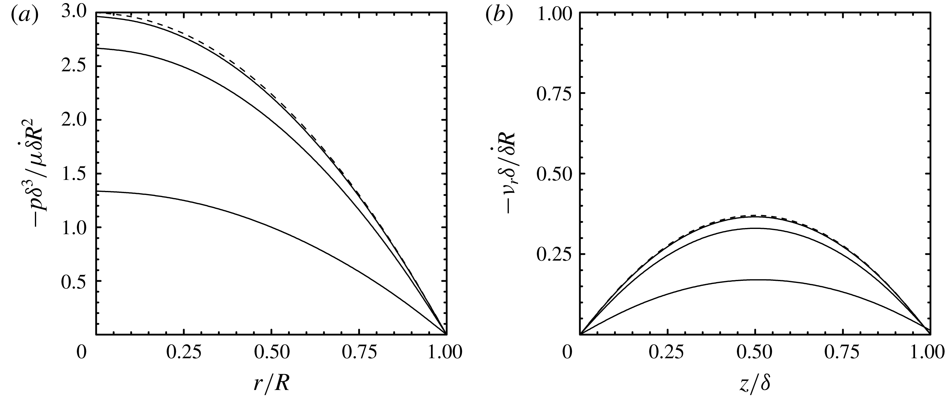
First, we consider the sealed-face configuration (i). Figure 2 shows the pressure and radial velocity fields in the liquid film for constant squeeze velocity
 $-\dot{\unicode[STIX]{x1D6FF}}$
. For the impermeable disk case (
 $\unicode[STIX]{x1D70E}=\unicode[STIX]{x1D6F6}=0$
), the expression in (2.22) gives
 $p\propto [1-(r/R)^{2}]$
and the expression in (2.24) gives
 $v_{r}\propto (r/R)[(z/\unicode[STIX]{x1D6FF})-(z/\unicode[STIX]{x1D6FF})^{2}]$
. From this figure we see that the pressure profile flattens, which, in turn, leads to a reduction in the radial velocity, as the permeability of the disk
 $\unicode[STIX]{x1D6F6}$
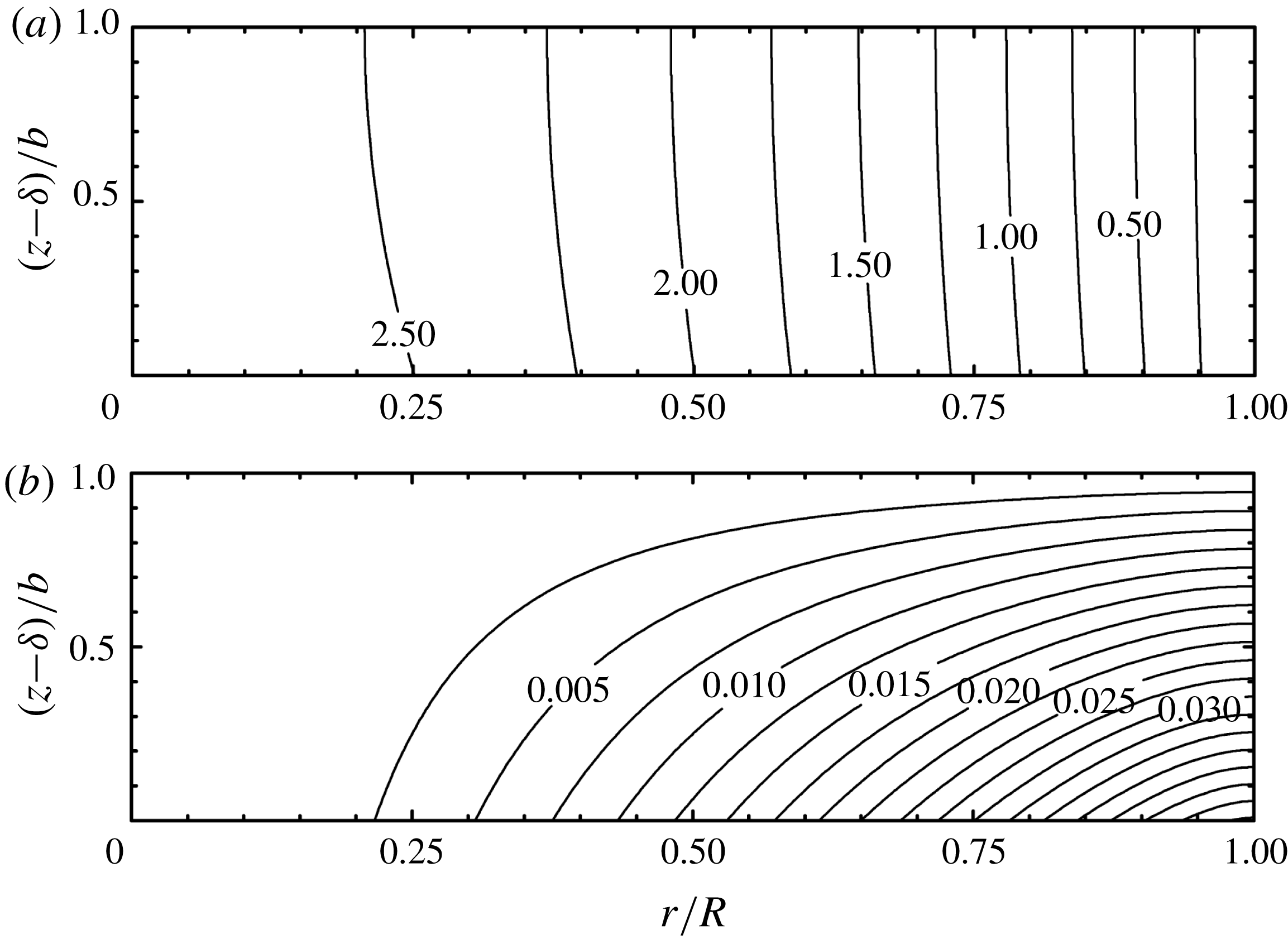
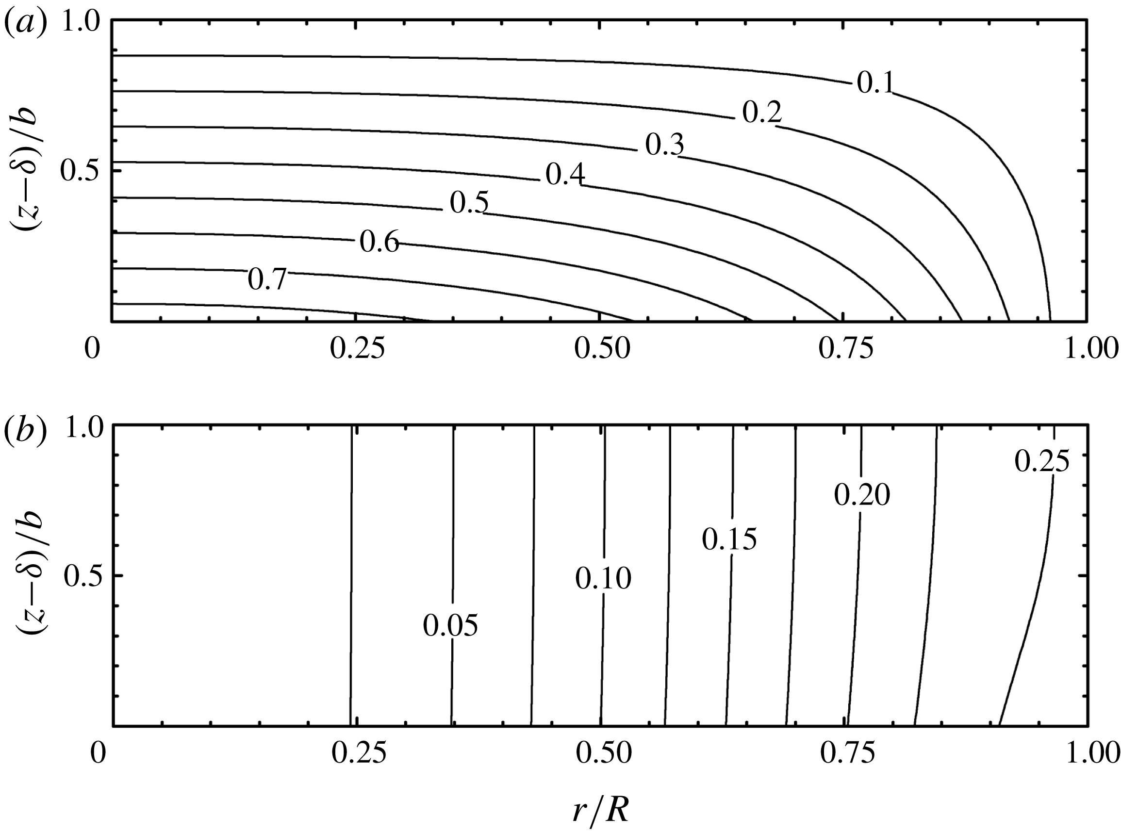
increases. Pressure and streamfunction contours within the porous disk are presented in figure 3, which shows that liquid flows into the porous disk axially and then, because of the impermeable upper surface, flows in the radial direction.
Pressure (a) from (2.22) and radial velocity at
 $r/R=0.5$
(b) from (2.24) in liquid film for configuration (i) with constant squeezing velocity
 $-\dot{\unicode[STIX]{x1D6FF}}$
for different values of permeability parameter
 $\unicode[STIX]{x1D6F6}=\unicode[STIX]{x1D705}R/\unicode[STIX]{x1D6FF}^{3}=0.01,0.1,1.0$
(solid lines top to bottom) with
 $\unicode[STIX]{x1D700}=0.1$
,
 $\unicode[STIX]{x1D6FF}/R=0.01$
and
 $\unicode[STIX]{x1D70E}=0$
. The dashed line is for the impermeable disk.
Pressure (a)
 $-\langle p\rangle _{i}\unicode[STIX]{x1D6FF}^{3}/\unicode[STIX]{x1D707}\dot{\unicode[STIX]{x1D6FF}}R^{2}$
from (2.23) and streamfunction (b)
 $-\langle \unicode[STIX]{x1D713}\rangle _{s}/\dot{\unicode[STIX]{x1D6FF}}R^{2}$
from (2.25) contours in a porous disk for configuration (i) with constant squeezing velocity
 $-\dot{\unicode[STIX]{x1D6FF}}$
for permeability parameter
 $\unicode[STIX]{x1D6F6}=\unicode[STIX]{x1D705}R/\unicode[STIX]{x1D6FF}^{3}=0.1$
with
 $\unicode[STIX]{x1D700}=0.1$
,
 $\unicode[STIX]{x1D6FF}/R=0.01$
and
 $\unicode[STIX]{x1D70E}=0$
.

We now examine the sealed-edge configuration (ii) for the case where
 $p_{0}=0$
so that liquid flows from the porous disk to the reservoir. Again, for the impermeable disk case (
 $\unicode[STIX]{x1D70E}=\unicode[STIX]{x1D6F6}=0$
), the expression in (2.36) simplifies to
 $p\propto [1-(r/R)^{2}]$
and the expression in (2.39) simplifies to
 $v_{r}\propto (r/R)[(z/\unicode[STIX]{x1D6FF})-(z/\unicode[STIX]{x1D6FF})^{2}]$
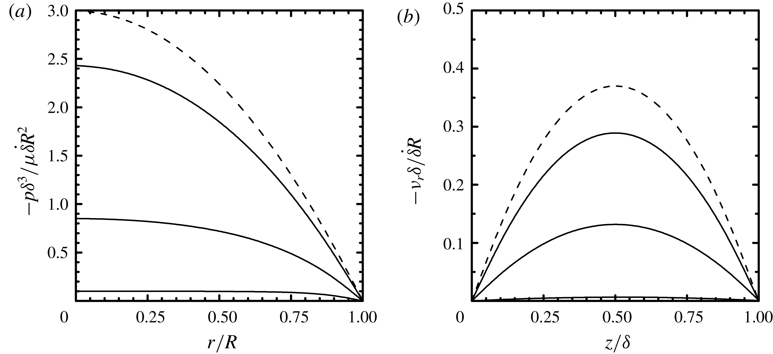
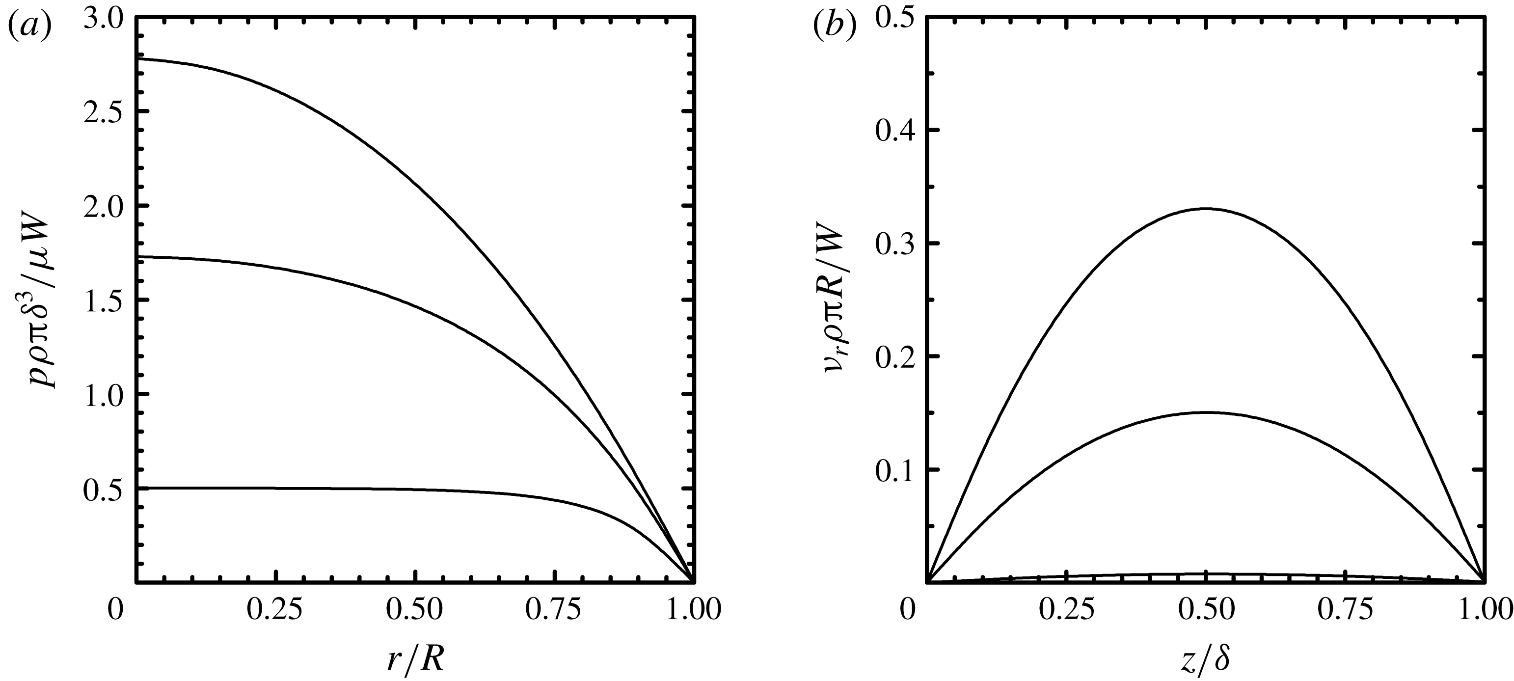
. Figure 4 shows the pressure and radial velocity fields in the liquid film for constant squeeze velocity
 $-\dot{\unicode[STIX]{x1D6FF}}$
. As with configuration (i), the pressure profile flattens and the radial velocity decreases as
 $\unicode[STIX]{x1D6F6}$
increases; however, the dependence on
 $\unicode[STIX]{x1D6F6}$
is stronger for configuration (ii) compared to configuration (i). For large permeability (
 $\unicode[STIX]{x1D6F6}=1.0$
), the liquid-film pressure is nearly uniform and the radial velocity approaches zero.
Pressure (a) from (2.36) and radial velocity at
 $r/R=0.5$
(b) from (2.39) for configuration (ii) with constant squeezing velocity
 $-\dot{\unicode[STIX]{x1D6FF}}$
for different values of permeability parameter
 $\unicode[STIX]{x1D6F6}=\unicode[STIX]{x1D705}R/\unicode[STIX]{x1D6FF}^{3}=0.01$
, 0.1, 1.0 (solid lines top to bottom) with
 $\unicode[STIX]{x1D700}=0.1$
,
 $\unicode[STIX]{x1D6FF}/R=0.01$
and
 $\unicode[STIX]{x1D70E}=0$
. The dashed line is for the impermeable disk.

As noted earlier, approximate solutions for configuration (ii) have been reported (Murti Reference Murti1974a
; Verma Reference Verma1980) by assuming
 $\langle p\rangle _{i}$
is a linear function of
 $z$
. In this case, the pressure within the porous disk is found using the boundary conditions in (2.12) and (2.27) and is given by
 $\langle p\rangle _{i}=p_{0}+(p_{0}-p)[(z-\unicode[STIX]{x1D6FF})/b-1]$
. We note, however, that this solution is not consistent with (2.8), (2.10a
) and (2.10b
). Nevertheless, using this assumption (and setting
 $p_{0}=0$
,
 $\unicode[STIX]{x1D70E}=0$
) the solution of (2.13) can be written as
 $$\begin{eqnarray}\frac{p\unicode[STIX]{x1D6FF}^{3}}{\unicode[STIX]{x1D707}R^{2}}=-\dot{\unicode[STIX]{x1D6FF}}\frac{\unicode[STIX]{x1D700}}{\unicode[STIX]{x1D6F6}}\left[1-\frac{\text{I}_{0}(\sqrt{12\unicode[STIX]{x1D6F6}/\unicode[STIX]{x1D700}}r/R)}{\text{I}_{0}(\sqrt{12\unicode[STIX]{x1D6F6}/\unicode[STIX]{x1D700}})}\right],\end{eqnarray}$$
where
 $\text{I}_{0}(x)$
is the modified Bessel function of the first kind. This expression is in good agreement with (2.36) for
 $\unicode[STIX]{x1D700}\ll 1$
, but over-predicts the liquid-film pressure for larger
 $\unicode[STIX]{x1D700}$
.
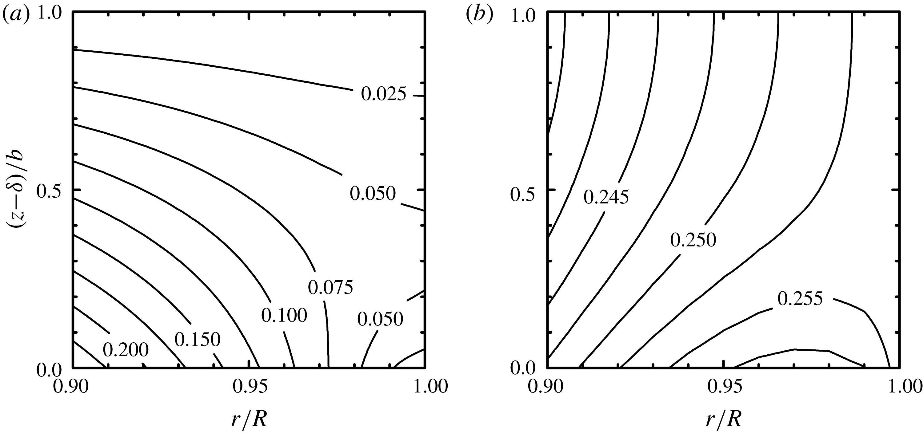
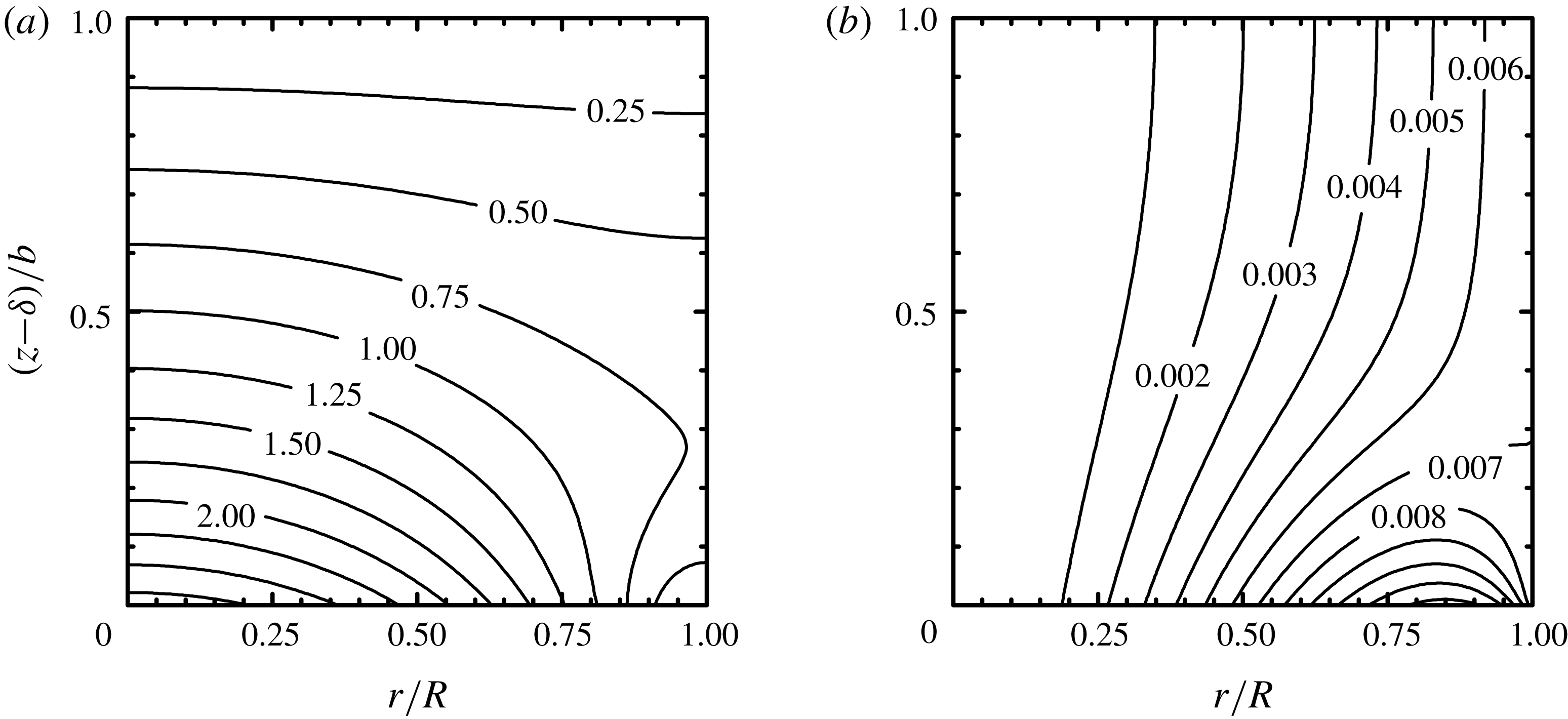
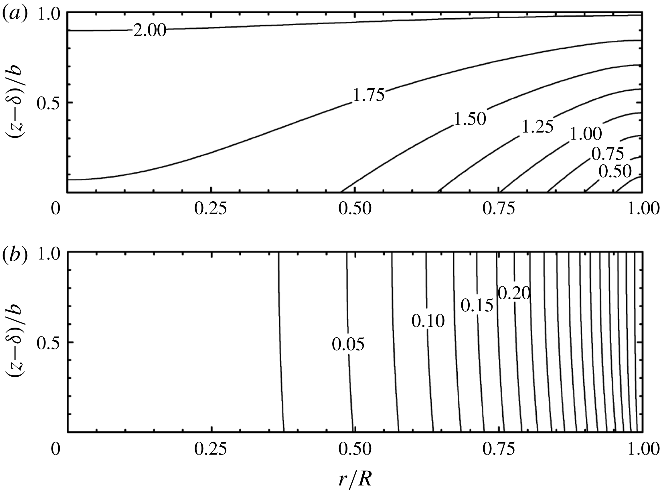
Pressure and streamfunction contours within the porous disk for configuration (ii) are presented in figure 5. From this figure we see that flow in the porous disk is mainly in the axial direction except near the outer edge of the disk. The detailed view given in figure 6 shows the flow splits where a portion of the liquid (for
 $r/R\gtrsim 0.93$
) entering the porous disk from the film flows back into the film, that is
 $\langle v_{z}\rangle _{s}(r,\unicode[STIX]{x1D6FF})<0$
. This occurs because liquid flow in the radial direction encounters the impermeable surface at
 $r=R$
, which results in a stagnation point. Hence, the flow resistance along a path back to liquid film is smaller than along a path through the porous disk to the reservoir. Pressure and streamfunction contours for a thick porous disk (
 $\unicode[STIX]{x1D700}=1$
) are presented in figure 5. Here, we see a rather pronounced flow splitting where fluid entering the disk for
 $r/R\gtrsim 0.55$
returns to the liquid film. The approximate solution where
 $\langle p\rangle _{i}$
is assumed to be a linear function of
 $z$
does not capture the more complicated pressure contours given by the exact solution, nor will it predict the flow splitting that is shown in figures 6 and 7. From (2.10b
) and (2.23), it is easy to show that
 $\langle v_{z}\rangle _{s}(r,\unicode[STIX]{x1D6FF})>0$
for
 $0\leqslant r\leqslant R$
, which means that for configuration (i), fluid within the porous disk never flows back into the liquid film. For configuration (ii), however, flow splitting becomes more pronounced with decreasing
 $\unicode[STIX]{x1D6F6}$
and vanishes only in the limit
 $\unicode[STIX]{x1D700}\rightarrow 0$
.
Pressure (a)
 $-\langle p\rangle _{i}\unicode[STIX]{x1D6FF}^{3}/\unicode[STIX]{x1D707}\dot{\unicode[STIX]{x1D6FF}}R^{2}$
from (2.38) and streamfunction (b)
 $-\langle \unicode[STIX]{x1D713}\rangle _{s}/\dot{\unicode[STIX]{x1D6FF}}R^{2}$
from (2.40) contours in a porous disk for configuration (ii) with constant squeezing velocity
 $-\dot{\unicode[STIX]{x1D6FF}}$
for permeability parameter
 $\unicode[STIX]{x1D6F6}=\unicode[STIX]{x1D705}R/\unicode[STIX]{x1D6FF}^{3}=0.1$
with
 $\unicode[STIX]{x1D700}=0.1$
,
 $\unicode[STIX]{x1D6FF}/R=0.01$
and
 $\unicode[STIX]{x1D70E}=0$
.

Detailed view of pressure (a)
 $-\langle p\rangle _{i}\unicode[STIX]{x1D6FF}^{3}/\unicode[STIX]{x1D707}\dot{\unicode[STIX]{x1D6FF}}R^{2}$
from (2.38) and streamfunction (b)
 $-\langle \unicode[STIX]{x1D713}\rangle _{s}/\dot{\unicode[STIX]{x1D6FF}}R^{2}$
from (2.40) contours in a porous disk for configuration (ii) with constant squeezing velocity
 $-\dot{\unicode[STIX]{x1D6FF}}$
for permeability parameter
 $\unicode[STIX]{x1D6F6}=\unicode[STIX]{x1D705}R/\unicode[STIX]{x1D6FF}^{3}=0.1$
with
 $\unicode[STIX]{x1D700}=0.1$
,
 $\unicode[STIX]{x1D6FF}/R=0.01$
and
 $\unicode[STIX]{x1D70E}=0$
.

Pressure (a)
 $-\langle p\rangle _{i}\unicode[STIX]{x1D6FF}^{3}/\unicode[STIX]{x1D707}\dot{\unicode[STIX]{x1D6FF}}R^{2}$
from (2.38) and streamfunction (b)
 $-\langle \unicode[STIX]{x1D713}\rangle _{s}/\dot{\unicode[STIX]{x1D6FF}}R^{2}$
from (2.40) contours in a porous disk for configuration (ii) with constant squeezing velocity
 $-\dot{\unicode[STIX]{x1D6FF}}$
for permeability parameter
 $\unicode[STIX]{x1D6F6}=\unicode[STIX]{x1D705}R/\unicode[STIX]{x1D6FF}^{3}=0.1$
with
 $\unicode[STIX]{x1D700}=1$
,
 $\unicode[STIX]{x1D6FF}/R=0.01$
and
 $\unicode[STIX]{x1D70E}=0$
.

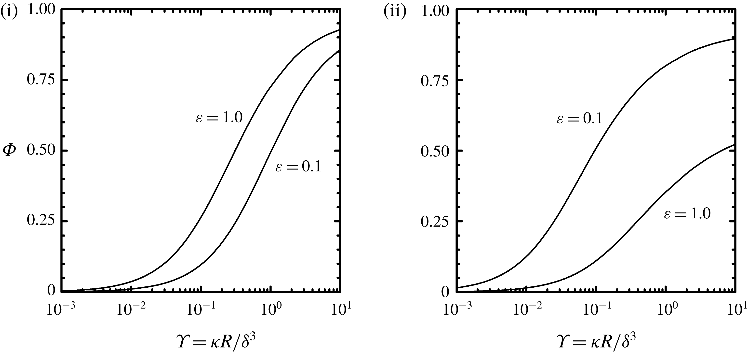
It is of interest to examine the rate at which the liquid flows into the porous disk relative to the rate at which it flows from the liquid film at
 $r=R$
. To examine this quantitatively, we consider the fraction of liquid from the film that flows into the porous disk for constant squeeze velocity
 $-\dot{\unicode[STIX]{x1D6FF}}$
, which is defined as
 $$\begin{eqnarray}\unicode[STIX]{x1D6F7}=-\frac{1}{\dot{\unicode[STIX]{x1D6FF}}}\frac{2}{R^{2}}\int _{0}^{R}\langle v_{z}\rangle _{s}(r,\unicode[STIX]{x1D6FF})r\,\text{d}r=\frac{\unicode[STIX]{x1D705}}{\unicode[STIX]{x1D707}\dot{\unicode[STIX]{x1D6FF}}}\frac{2}{R^{2}}\int _{0}^{R}\frac{\unicode[STIX]{x2202}\langle p\rangle _{i}}{\unicode[STIX]{x2202}z}(r,\unicode[STIX]{x1D6FF})r\,\text{d}r,\end{eqnarray}$$
where the second equality follows using (2.10b
). The fraction of liquid that flows, or is squeezed, out of the film at
 $r=R$
is
 $1-\unicode[STIX]{x1D6F7}$
; for the case of an impermeable disk,
 $\unicode[STIX]{x1D6F7}=0$
. The dependence of
 $\unicode[STIX]{x1D6F7}$
on
 $\unicode[STIX]{x1D6F6}$
for configurations (i) and (ii) is shown in figure 8. For constant squeeze velocity
 $-\dot{\unicode[STIX]{x1D6FF}}$
, since the film thickness
 $\unicode[STIX]{x1D6FF}$
decreases (
 $\unicode[STIX]{x1D6F6}$
increases),
 $\unicode[STIX]{x1D6F7}$
increases during squeezing. In figure 8 we see for a thin porous disk (
 $\unicode[STIX]{x1D700}=0.1$
) that
 $\unicode[STIX]{x1D6F7}$
is larger for configuration (ii) compared with configuration (i), and the opposite is true for a thick porous disk (
 $\unicode[STIX]{x1D700}=1.0$
). This is explained by the fact that increasing the disk thickness for configuration (ii) leads to a larger resistance for flow to the reservoir, while for configuration (i) an increase in
 $\unicode[STIX]{x1D700}$
lowers the resistance for flow out of the disk at
 $r=R$
. Figure 8 also shows that the dependence of
 $\unicode[STIX]{x1D6F7}$
on disk thickness
 $\unicode[STIX]{x1D700}$
is stronger for configuration (ii) compared to (i). As we have just seen (see figures 6 and 7), the degree of flow separation and flow from the porous disk back into the film (
 $\langle v_{z}\rangle _{s}(r,\unicode[STIX]{x1D6FF})<0$
) for configuration (ii) increases with increasing
 $\unicode[STIX]{x1D700}$
.
Fraction of liquid from the film that flows into the porous disk as defined in (3.2) for configurations (i) and (ii) with constant squeezing velocity
 $-\dot{\unicode[STIX]{x1D6FF}}$
as a function of permeability parameter
 $\unicode[STIX]{x1D6F6}=\unicode[STIX]{x1D705}R/\unicode[STIX]{x1D6FF}^{3}$
for
 $\unicode[STIX]{x1D70E}=0$
and
 $\unicode[STIX]{x1D6FF}/R=0.01$
.

As noted in the previous section, the sealed-edge configuration (ii) includes the case of an externally pressurized bearing where the mass flow rate
 ${\mathcal{W}}$
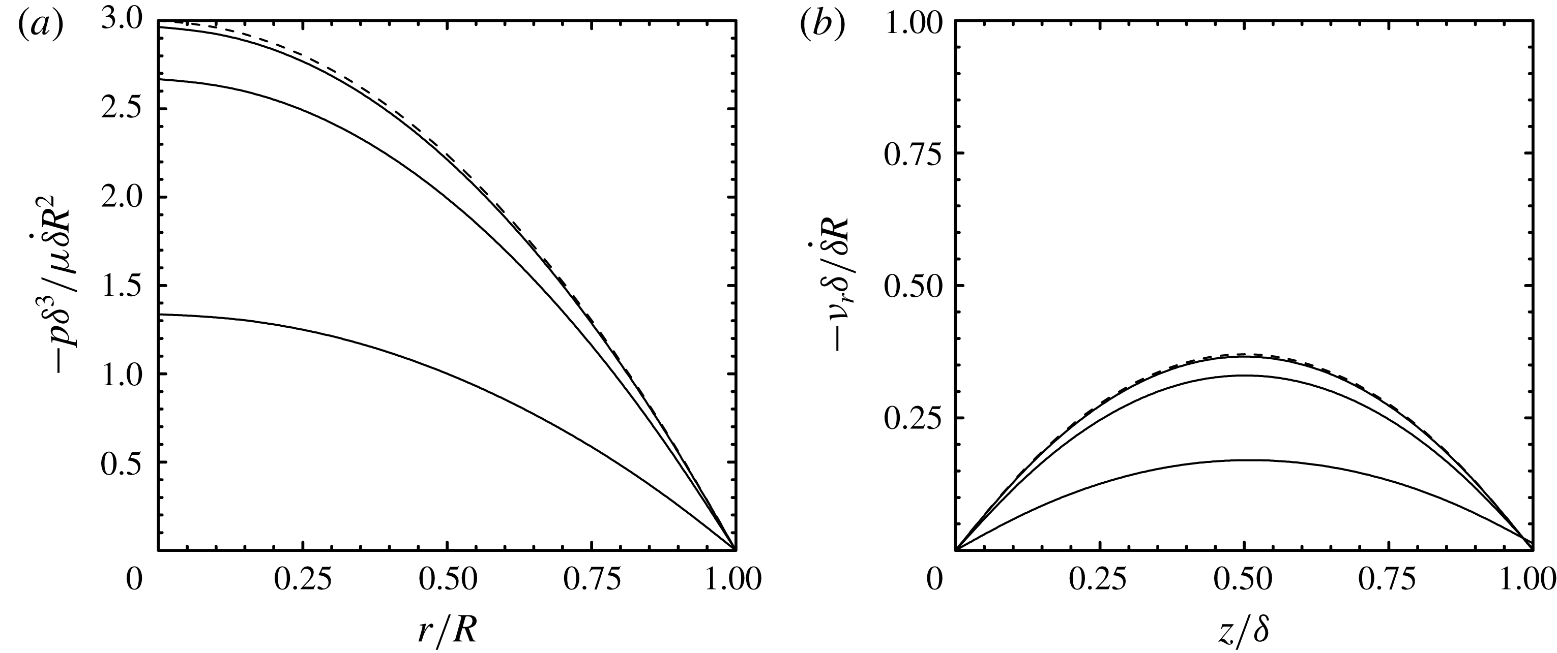
from the reservoir to the porous disk is prescribed. Figure 9 shows the pressure and radial velocity fields in the liquid film for the case of a constant film thickness (
 $\dot{\unicode[STIX]{x1D6FF}}=0$
). From this figure we again see that the pressure profile flattens and radial velocity decreases as
 $\unicode[STIX]{x1D6F6}$
increases (see figure 4). Pressure and streamfunction contours within the porous disk for this case are presented in figure 10, which shows that the pressure field varies primarily in the axial direction leading to a flow in the axial direction. The modification of the lubricated squeezing flow technique for generating equibiaxial deformations in polymer melts (Venerus et al.
Reference Venerus, Shiu, Kashyap and Hosttetler2010) is based on this type of flow where the liquid (lubricant) film thickness is constant.
Pressure (a) from (2.36) and radial velocity at
 $r/R=0.5$
(b) from (2.39) for configuration (ii) with constant
 ${\mathcal{W}}$
and
 $\dot{\unicode[STIX]{x1D6FF}}=0$
for permeability parameter
 $\unicode[STIX]{x1D6F6}=\unicode[STIX]{x1D705}R/\unicode[STIX]{x1D6FF}^{3}=0.01$
, 0.1, 1.0 (solid lines top to bottom) with
 $\unicode[STIX]{x1D700}=0.1$
,
 $\unicode[STIX]{x1D6FF}/R=0.01$
and
 $\unicode[STIX]{x1D70E}=0$
.

Pressure (a)
 $\langle p\rangle _{i}\unicode[STIX]{x1D70C}\unicode[STIX]{x03C0}\unicode[STIX]{x1D6FF}^{3}/\unicode[STIX]{x1D707}{\mathcal{W}}$
from (2.38) and streamfunction (b)
 $\langle \unicode[STIX]{x1D713}\rangle _{s}\unicode[STIX]{x1D70C}\unicode[STIX]{x03C0}/{\mathcal{W}}$
from (2.40) contours in a porous disk for configuration (ii) with constant
 ${\mathcal{W}}$
and
 $\dot{\unicode[STIX]{x1D6FF}}=0$
for permeability parameter
 $\unicode[STIX]{x1D6F6}=\unicode[STIX]{x1D705}R/\unicode[STIX]{x1D6FF}^{3}=0.1$
with
 $\unicode[STIX]{x1D700}=0.1$
,
 $\unicode[STIX]{x1D6FF}/R=0.01$
and
 $\unicode[STIX]{x1D70E}=0$
.

3.2 Load-bearing behaviour
It is of great interest to understand the load-bearing behaviour of porous-walled thrust bearings and its dependence on the properties of the porous disk. The force exerted on the permeable disk
 ${\mathcal{F}}$
is due to the pressure field that develops in the liquid film, which is required to drive flow in the radial direction. As a reference, we consider the impermeable disk case (
 $\unicode[STIX]{x1D70E}=\unicode[STIX]{x1D6F6}=0$
). For this case, expressions for
 ${\mathcal{F}}$
for configurations (i) and (ii) given in (2.26) and (2.43), respectively, simplify to
 $$\begin{eqnarray}\frac{2{\mathcal{F}}}{3\unicode[STIX]{x1D707}\unicode[STIX]{x03C0}R^{4}}=-\frac{\dot{\unicode[STIX]{x1D6FF}}}{\unicode[STIX]{x1D6FF}^{3}}.\end{eqnarray}$$
For constant squeezing velocity
 $-\dot{\unicode[STIX]{x1D6FF}}$
, we see that
 ${\mathcal{F}}\rightarrow \infty$
as
 $\unicode[STIX]{x1D6FF}\rightarrow 0$
.
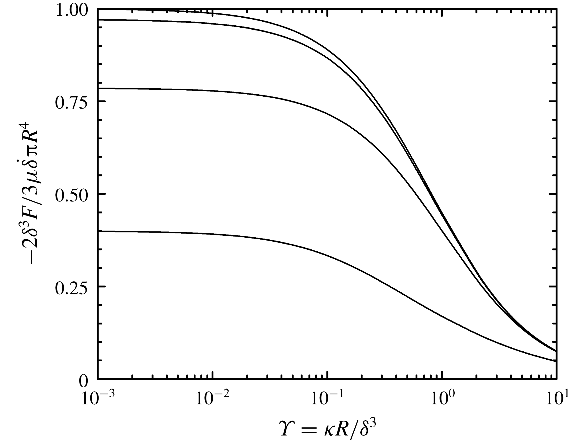
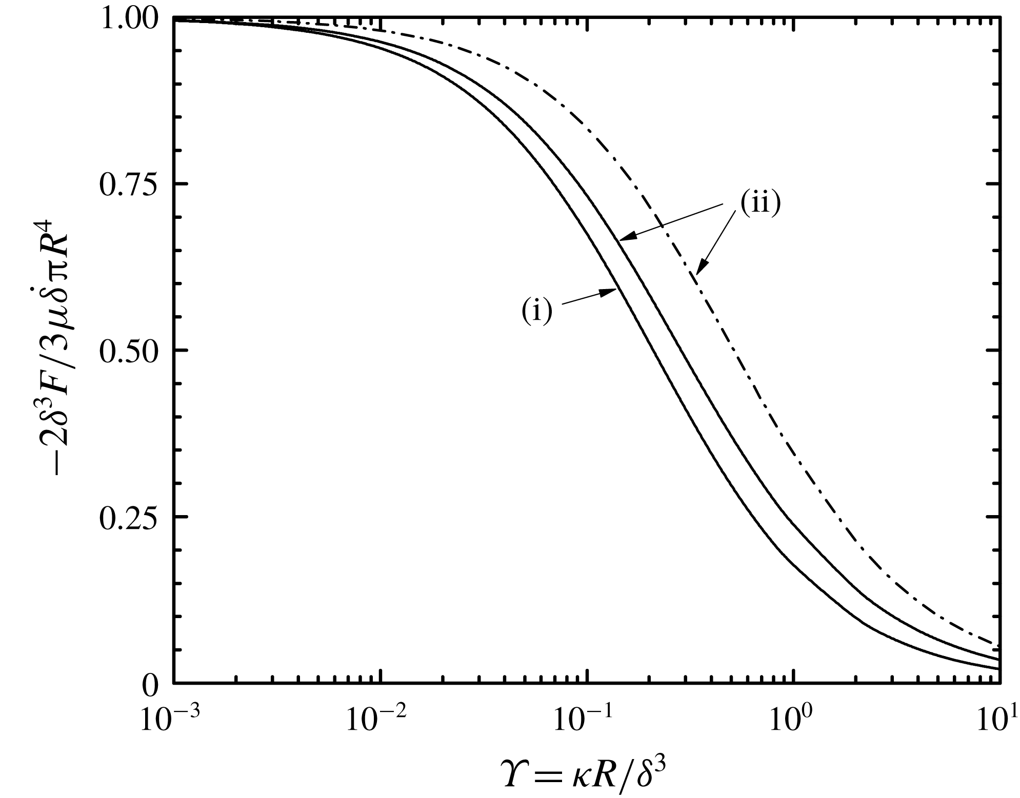
Figure 11 shows the dependence of force on the porous disk
 ${\mathcal{F}}$
on the permeability parameter
 $\unicode[STIX]{x1D6F6}$
for the sealed-face configuration (i). According to (3.3), we see that
 ${\mathcal{F}}$
is reduced relative to the impermeable disk case. The load-bearing capacity is further reduced by slip as shown by the dependence of
 ${\mathcal{F}}$
on
 $\unicode[STIX]{x1D70E}$
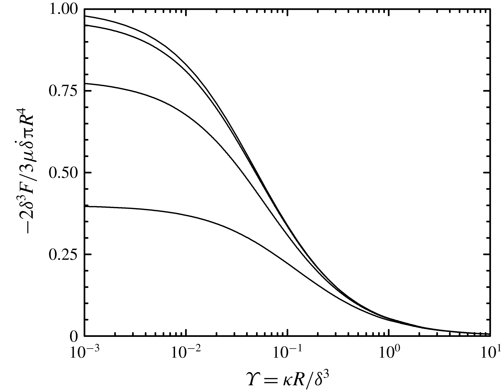
. Results for the sealed-edge configuration (ii) with
 $p_{0}=0$
are presented in figure 12, where it is evident that
 ${\mathcal{F}}$
is also reduced relative to the impermeable disk case and is further reduced by slip. Comparison of figures 11 and 12 shows that, for a thin porous disk
 $\unicode[STIX]{x1D700}=0.1$
, the load-bearing capacity of configuration (ii) is smaller than configuration (i). For example, for
 $\unicode[STIX]{x1D6F6}=1$
, the load-bearing capacity of configuration (ii) is roughly a factor of 10 smaller than configuration (i). The dependence of
 ${\mathcal{F}}$
on
 $\unicode[STIX]{x1D6F6}$
in these figures can be understood when one considers the results in figure 8, which show that increasing
 $\unicode[STIX]{x1D6F6}$
leads to an increase in
 $\unicode[STIX]{x1D6F7}$
, thereby reducing the radial velocity (and pressure) in the liquid film.
Force on porous disk from (2.26) for configuration (i) with constant squeezing velocity
 $-\dot{\unicode[STIX]{x1D6FF}}$
as a function of permeability parameter
 $\unicode[STIX]{x1D6F6}=\unicode[STIX]{x1D705}R/\unicode[STIX]{x1D6FF}^{3}$
for different values of slip parameter
 $\unicode[STIX]{x1D70E}=\sqrt{\unicode[STIX]{x1D705}}/\unicode[STIX]{x1D6FF}\unicode[STIX]{x1D6FC}=0$
, 0.01, 0.1, 1.0 (solid lines top to bottom) with
 $\unicode[STIX]{x1D700}=0.1$
and
 $\unicode[STIX]{x1D6FF}/R=0.01$
.

Force on porous disk from (2.43) for configuration (ii) with constant squeezing velocity
 $-\dot{\unicode[STIX]{x1D6FF}}$
as a function of permeability parameter
 $\unicode[STIX]{x1D6F6}=\unicode[STIX]{x1D705}R/\unicode[STIX]{x1D6FF}^{3}$
for different values of slip parameter
 $\unicode[STIX]{x1D70E}=\sqrt{\unicode[STIX]{x1D705}}/\unicode[STIX]{x1D6FF}\unicode[STIX]{x1D6FC}=0$
, 0.01, 0.1, 1.0 (solid lines top to bottom) with
 $\unicode[STIX]{x1D700}=0.1$
and
 $\unicode[STIX]{x1D6FF}/R=0.01$
.

The load-bearing behaviours of configurations (i) and (ii) for a thick porous disk (
 $\unicode[STIX]{x1D700}=1$
) are presented in figure 13. A comparison of these results with those in figures 11 and 12 indicates that increasing
 $\unicode[STIX]{x1D700}$
leads to a reduction in the load-bearing capacity for configuration (i) and an increase in the load-bearing capacity for configuration (ii). The latter is explained by the fact that for configuration (ii) the flow is primarily in the axial direction and an increase in porous disk thickness requires a larger pressure in the liquid film to drive the flow. For configuration (i), an increase in disk thickness moves the impermeable upper surface away from the liquid film, thereby decreasing the pressure required to drive flow through the porous disk at permeable external surfaces. The load-bearing capacities of configurations (i) and (ii) coincide for
 $\unicode[STIX]{x1D700}\approx 0.6$
.
An expression for
 ${\mathcal{F}}$
using the approximate solution described above is obtained by substitution of (3.1) in (2.14) leading to
 $$\begin{eqnarray}\frac{2{\mathcal{F}}}{3\unicode[STIX]{x1D707}\unicode[STIX]{x03C0}R^{4}}=-\frac{\dot{\unicode[STIX]{x1D6FF}}}{\unicode[STIX]{x1D6FF}^{3}}\frac{2\unicode[STIX]{x1D700}}{3\unicode[STIX]{x1D6F6}}\left[1-\frac{2\text{I}_{1}(\sqrt{12\unicode[STIX]{x1D6F6}/\unicode[STIX]{x1D700}})}{\sqrt{12\unicode[STIX]{x1D6F6}/\unicode[STIX]{x1D700}}\text{I}_{0}(\sqrt{12\unicode[STIX]{x1D6F6}/\unicode[STIX]{x1D700}})}\right],\end{eqnarray}$$
which is equivalent to the expression given by Verma (Reference Verma1980). For thin porous disks
 $\unicode[STIX]{x1D700}\ll 1$
, predictions for
 ${\mathcal{F}}$
from (3.4) are consistent with those from the exact solution in (2.43). However, as shown in figure 13 for
 $\unicode[STIX]{x1D700}=1$
, the expression in (3.4) from the approximate model significantly over-predicts
 ${\mathcal{F}}$
.
Force on porous disk from (2.26) for configuration (i) and from (2.43) for configuration (ii) with constant squeezing velocity
 $-\dot{\unicode[STIX]{x1D6FF}}$
as a function of permeability parameter
 $\unicode[STIX]{x1D6F6}=\unicode[STIX]{x1D705}R/\unicode[STIX]{x1D6FF}^{3}$
for
 $\unicode[STIX]{x1D70E}=0$
with
 $\unicode[STIX]{x1D700}=1.0$
and
 $\unicode[STIX]{x1D6FF}/R=0.01$
. The dashed curve is the approximate solution for configuration (ii) given in (3.4).

We now examine the dynamics of liquid-film thinning for constant applied force
 ${\mathcal{F}}$
. Again, we use the impermeable case as a reference. Integration of (3.3) with
 $\unicode[STIX]{x1D6FF}(0)=\unicode[STIX]{x1D6FF}_{0}$
gives
 $$\begin{eqnarray}\frac{\unicode[STIX]{x1D6FF}}{\unicode[STIX]{x1D6FF}_{0}}=\frac{1}{\sqrt{1+4{\mathcal{F}}\unicode[STIX]{x1D6FF}_{0}^{2}t/3\unicode[STIX]{x1D707}\unicode[STIX]{x03C0}R^{4}}},\end{eqnarray}$$
which shows that
 $\unicode[STIX]{x1D6FF}\rightarrow 0$
only for
 $t\rightarrow \infty$
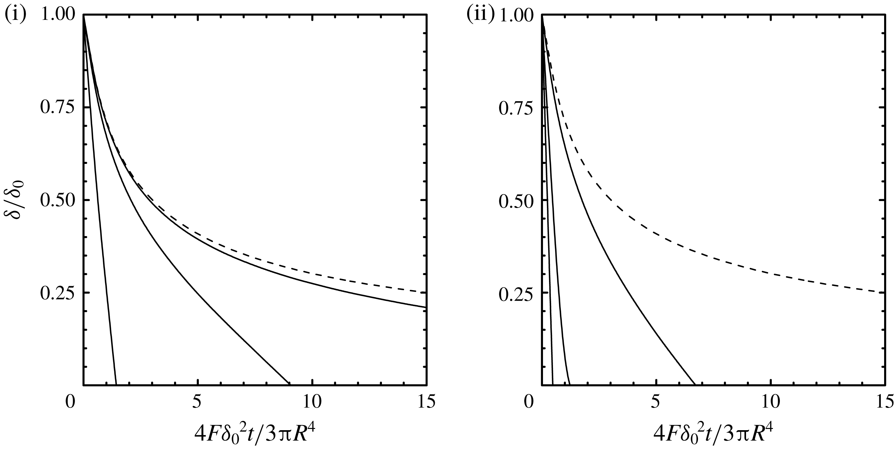
. Figure 14 shows the liquid-film thickness as a function of time for configurations (i) and (ii) without a slip velocity (
 $\unicode[STIX]{x1D70E}=0$
) for different values of the permeability parameter
 $\unicode[STIX]{x1D6F6}=\unicode[STIX]{x1D705}R/\unicode[STIX]{x1D6FF}_{0}^{3}$
. These results were obtained by a straightforward numerical integration of (2.26) and (2.43) with
 $\unicode[STIX]{x1D6FF}(0)=\unicode[STIX]{x1D6FF}_{0}$
. As expected the rate of liquid-film drainage is increased relative to the impermeable case, and, for
 $\unicode[STIX]{x1D700}=0.1$
, the rate of drainage is larger for configuration (ii) compared to configuration (i). Including a slip velocity (
 $\unicode[STIX]{x1D70E}\neq 0$
) decreases
 ${\mathcal{F}}$
(see figures 11 and 12) and would further increase the rate of liquid film drainage. From figure 14 we see that complete drainage of the liquid film occurs at a finite time, which we denote as
 $t_{f}$
:
 $\unicode[STIX]{x1D6FF}(t_{f})=0$
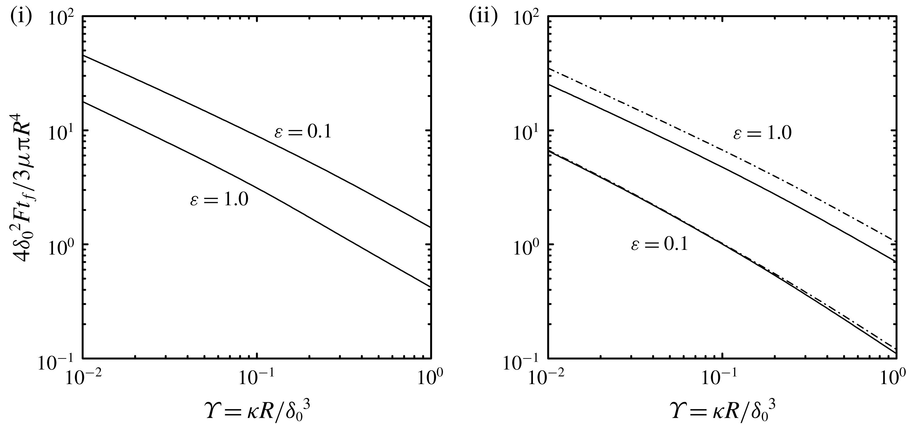
. The dependence of
 $t_{f}$
on the permeability parameter
 $\unicode[STIX]{x1D6F6}=\unicode[STIX]{x1D705}R/\unicode[STIX]{x1D6FF}_{0}^{3}$
for configurations (i) and (ii) for
 $\unicode[STIX]{x1D700}=0.1,1$
is shown in figure 15. As expected,
 $t_{f}$
decreases with increasing permeability
 $\unicode[STIX]{x1D6F6}$
, which was previously reported for configuration (i) (Murti Reference Murti1974b
; Knox et al.
Reference Knox, Wilson, Duffy and McKee2015). For configuration (i) we see that increasing the thickness of the porous disk
 $\unicode[STIX]{x1D700}$
decreases the time for complete film drainage, while for configuration (ii) increasing
 $\unicode[STIX]{x1D700}$
leads to an increase in
 $t_{f}$
. Also shown in figure 15 is
 $t_{f}$
from the approximate solution for configuration (ii) determined by numerical integration of (3.4), which over-predicts
 $t_{f}$
for the thicker porous disk
 $\unicode[STIX]{x1D700}=1$
.
Liquid-film thickness as a function of time from (2.26) for configuration (i) and from (2.43) for configuration (ii) with constant squeezing force
 ${\mathcal{F}}$
for different values of permeability parameter
 $\unicode[STIX]{x1D6F6}=\unicode[STIX]{x1D705}R/\unicode[STIX]{x1D6FF}_{0}^{3}=0.01$
, 0.1, 1.0 (solid lines top to bottom) with
 $\unicode[STIX]{x1D700}=0.1$
,
 $\unicode[STIX]{x1D6FF}_{0}/R=0.01$
and
 $\unicode[STIX]{x1D70E}=0$
. The dashed line is for the impermeable disk given by (3.5).

Time for complete drainage of liquid-film thickness
 $\unicode[STIX]{x1D6FF}(t_{f})=0$
for configurations (i) and (ii) with constant squeezing force
 ${\mathcal{F}}$
as a function of permeability parameter
 $\unicode[STIX]{x1D6F6}=\unicode[STIX]{x1D705}R/\unicode[STIX]{x1D6FF}_{0}^{3}$
with
 $\unicode[STIX]{x1D700}=0.1,1.0$
,
 $\unicode[STIX]{x1D6FF}_{0}/R=0.01$
and
 $\unicode[STIX]{x1D70E}=0$
. The dot-dashed line is for the approximate solution from (3.4).

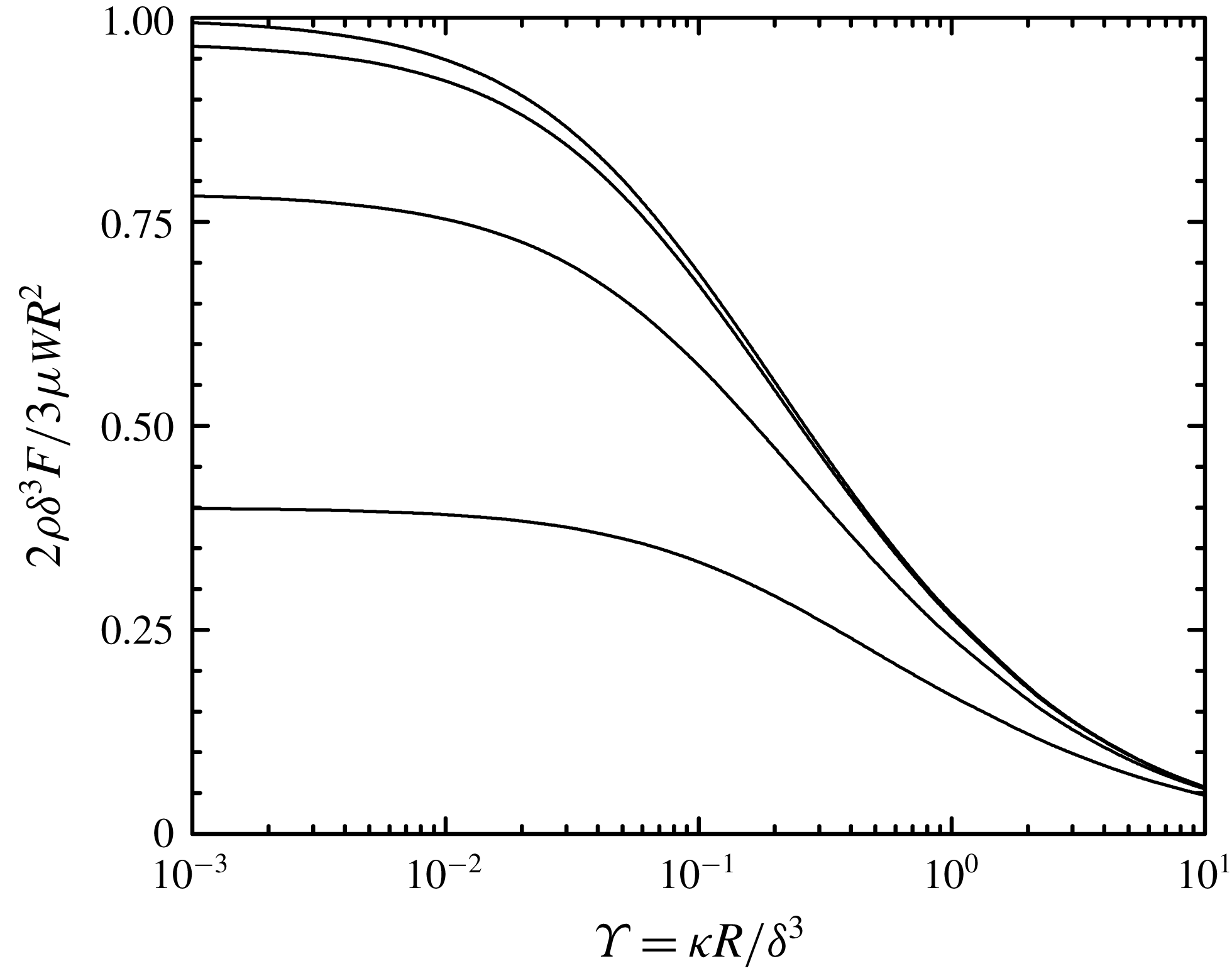
Finally, we consider the load-bearing characteristics of configuration (ii) when the liquid mass flow rate
 ${\mathcal{W}}$
from the reservoir to the porous disk is prescribed, or an externally pressurized bearing. This allows for a thrust bearing where the liquid film thickness can be controlled. Figure 16 shows the dependence of the load-bearing capacity on the permeability parameter
 $\unicode[STIX]{x1D6F6}$
for constant
 ${\mathcal{W}}$
with constant liquid-film thickness (
 $\dot{\unicode[STIX]{x1D6FF}}=0$
). From this figure we see that
 ${\mathcal{F}}$
decreases with increasing disk permeability
 $\unicode[STIX]{x1D6F6}$
and that a slip velocity further reduces load-bearing capacity. While
 ${\mathcal{F}}$
increases with decreasing
 $\unicode[STIX]{x1D6F6}$
, the reservoir pressure
 $p_{0}$
, which can be computed from (2.37), increases.
Force on porous disk from (2.41) for configuration (ii) with constant
 ${\mathcal{W}}$
and
 $\dot{\unicode[STIX]{x1D6FF}}=0$
as a function of permeability parameter
 $\unicode[STIX]{x1D6F6}=\unicode[STIX]{x1D705}R/\unicode[STIX]{x1D6FF}^{3}$
for different values of slip parameter
 $\unicode[STIX]{x1D70E}=\sqrt{\unicode[STIX]{x1D705}}/\unicode[STIX]{x1D6FF}\unicode[STIX]{x1D6FC}=0$
, 0.01, 0.1, 1.0 (solid lines top to bottom) with
 $\unicode[STIX]{x1D700}=0.1$
and
 $\unicode[STIX]{x1D6FF}/R=0.01$
.

When operated with a prescribed liquid mass flow rate, the thrust bearing can also be used to lift an applied load. To demonstrate this, (2.41) is numerically integrated with the initial condition
 $\unicode[STIX]{x1D6FF}(0)=0$
; the constant applied force
 ${\mathcal{F}}$
is set by the expression in (2.41) at steady state (
 $\dot{\unicode[STIX]{x1D6FF}}=0$
) and depends on the final liquid-film thickness
 $\unicode[STIX]{x1D6FF}(t\rightarrow \infty )=\unicode[STIX]{x1D6FF}_{\infty }$
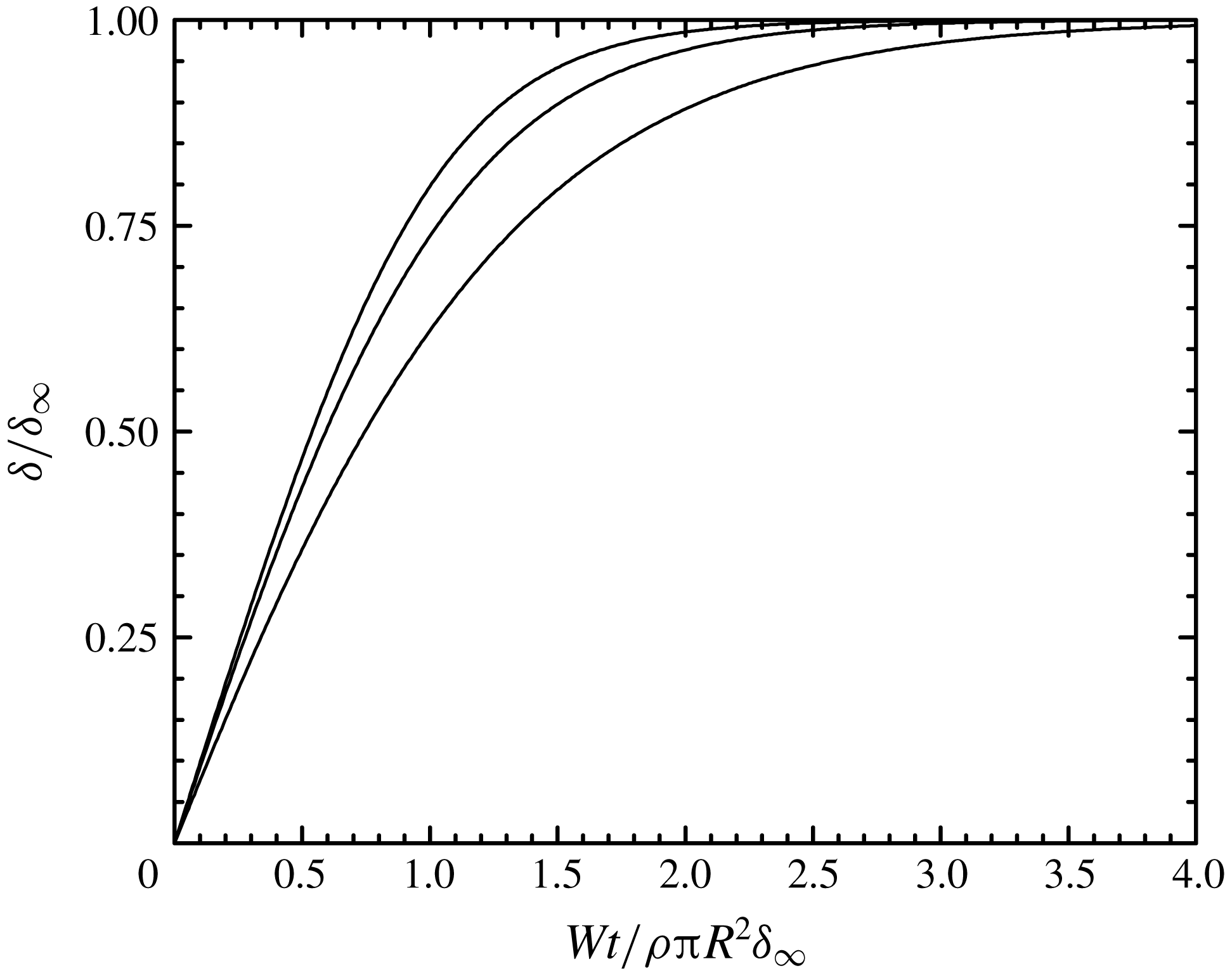
. As shown in figure 17, prescribing a constant
 ${\mathcal{W}}$
causes the liquid-film thickness to increase, lifting the load, to the final liquid-film thickness
 $\unicode[STIX]{x1D6FF}_{\infty }$
. Alternatively, one could examine the time evolution of the film thickness if the reservoir pressure
 $p_{0}$
were prescribed, and
 ${\mathcal{W}}$
would be determined by (2.37).
Liquid-film thickness as a function of time by integration of (2.41) for configuration (ii) with constant
 ${\mathcal{W}}$
for different values of permeability parameter
 $\unicode[STIX]{x1D6F6}=\unicode[STIX]{x1D705}R/\unicode[STIX]{x1D6FF}_{\infty }^{3}=0.001$
, 0.01, 0.1 (solid lines top to bottom) with
 $\unicode[STIX]{x1D700}=0.1$
,
 $\unicode[STIX]{x1D6FF}_{\infty }/R=0.01$
and
 $\unicode[STIX]{x1D70E}=0$
. The squeezing force
 ${\mathcal{F}}$
is determined from figure 17 with
 $\unicode[STIX]{x1D6FF}\rightarrow \unicode[STIX]{x1D6FF}_{\infty }$
.

4 Summary
Squeeze flows in liquid films bound by a porous disk have been investigated for two configurations (see figure 1). In the sealed-face configuration (i), the upper surface of the porous disk is impermeable and in the sealed-edge configuration (ii), the upper surface of this disk is permeable and exposed to a reservoir having uniform pressure. For configuration (ii), it is possible to control the flow of liquid from the reservoir to the porous disk, or to allow liquid to flow out of the porous disk to the reservoir at ambient pressure making it similar to configuration (i). Analytical solutions of the coupled systems of equations governing flow in the porous disk (Darcy’s law) and liquid film (lubrication approximation) are obtained for both configurations leading to expressions for velocity and pressure fields as well as the force exerted on the porous disk.
Results have been obtained as a function of three dimensionless parameters that are determined by the disk permeability (
 $\unicode[STIX]{x1D6F6}$
) and geometry (
 $\unicode[STIX]{x1D700}$
) and by a slip velocity (
 $\unicode[STIX]{x1D70E}$
) at the interface between the porous disk and liquid film. Velocity and pressure fields in the liquid film are qualitatively the same in both configurations, while in the porous disk they can be qualitatively different under certain conditions. In particular, we show that for configuration (ii) where the reservoir is at ambient pressure, flow in the porous disk exhibits a stagnation point and flow separation where a portion of the liquid in the film flows into the porous disk and then back into the film. The fraction of the liquid in the film that flows through the porous disk (as opposed to being squeezed out of the liquid film) has a strong dependence on disk permeability (
 $\unicode[STIX]{x1D6F6}$
) and geometry (
 $\unicode[STIX]{x1D700}$
) with a qualitatively different dependence on the latter for configurations (i) and (ii).
The load-bearing capacity of configuration (i) and configuration (ii) with the reservoir at ambient pressure have been examined as a function of disk permeability and geometry and the magnitude of a slip velocity. The dependence on disk permeability (
 $\unicode[STIX]{x1D6F6}$
) is qualitatively similar for the two configurations, while the dependence on porous disk thickness (
 $\unicode[STIX]{x1D700}$
) is qualitatively different. In fact, we find that the load-bearing capacity of the two configurations with the same permeability is equal for a particular value of disk thickness. The presence of a slip velocity leads to a significant reduction in the load-bearing capacity for both configurations. We also demonstrate the range of applicability for predicting load-bearing capacity obtained from a previously published approximate model for configuration (ii). The dynamics of liquid-film thickness for a constant applied load has been investigated. We find that the time for the film thickness to vanish decreases with increasing disk permeability (
 $\unicode[STIX]{x1D6F6}$
) for both configurations (i) and (ii); it decreases with increasing disk thickness (
 $\unicode[STIX]{x1D700}$
) for configuration (i), and shows the opposite trend for configuration (ii). Finally, we have shown for configuration (ii) with a prescribed mass flow from the reservoir, that the liquid-film thickness can be controlled allowing the bearing to lift a constant load.
The results presented here have important consequences with regard to the design of thrust bearings where load-bearing characteristics can be tuned by appropriate choices of disk permeability and geometry. These results are also relevant to understanding the behaviour of diathrodial joints and approaches for their treatment and/or replacement.