1 INTRODUCTION
Jumps on the paths of efficient asset prices have important economic implications ranging from risk management to asset pricing (see, e.g., Andersen, Bollerslev, and Diebold, Reference Andersen, Bollerslev and Diebold2007; Tauchen and Zhou, Reference Tauchen and Zhou2011; Fulop, Li, and Yu, Reference Fulop, Li and Yu2015). Various statistical tests that detect the occurrences of jumps with high-frequency data have been proposed in the literature. Besides examining whether there are jumps within a fixed period (e.g., Corsi, Pirino, and Reno, Reference Corsi, Pirino and Reno2010; Aït-Sahalia, Jacod, and Li, Reference Aït-Sahalia, Jacod and Li2012), researchers can use high-frequency data to further identify jumps within small time intervals (e.g., Lee and Mykland, Reference Lee and Mykland2008, Reference Lee and Mykland2012). In this article, we develop a sequential testing procedure to locate jumps based on the randomization technique proposed by Corradi and Swanson (Reference Corradi and Swanson2006) and Trapani (Reference Trapani2018). Compared to the existing sequential tests for jumps, the proposed test has the advantage of being theoretically robust to discontinuous spot volatility and not relying on some spot volatility estimator which is required to be consistent across various time points, since such an estimator can be difficult to derive in the presence of the market microstructure noise. This article also contributes to the literature on randomized tests by deriving the extreme value theory for randomized statistics in building a global test which consists of many local ones.
We test for jumps with respect to overlapping time windows whose lengths diminish as more frequent observations are employed. For each of these windows, we use the Huber loss function to derive robust approximations of the locally averaged returns (LARs) of the efficient price, and the resultant statistics are called the robust LAR, which have been employed by Sun (Reference Sun2024) for jump tests. We then add some artificially generated randomness to the robust LAR in order to obtain the randomized statistics. Under certain regularity conditions, including assumptions of finite activity (FA) jumps and a fixed T (the length of the whole sampling period), we reveal the asymptotic behavior of the maximum of all the randomized statistics unaffected by jumps, and accordingly, set the threshold for rejecting the null hypothesis of no jumps, so that the limiting probability of the global type I error (GTE) equals the prescribed significance level. Furthermore, with probability approaching one, the proposed test can detect all jumps and locate them within small intervals. We also derive asymptotic theories to justify our test for cases where jumps have infinite activity (IA) or T goes to infinity as the sampling frequency becomes higher.
A strand of literature proposes sequential tests for jump detection where the statistics are obtained by standardizing the (locally averaged) intraday returns with some spot volatility estimator. This methodology is introduced by Andersen, Bollerslev, and Dobrev (Reference Andersen, Bollerslev and Dobrev2007) and Lee and Mykland (Reference Lee and Mykland2008), where volatility estimators derived from the bipower variation are used to standardize the intraday returns. Given the prevalence of the microstructure noise (cf. Hansen and Lunde, Reference Hansen and Lunde2006; Christensen, Oomen, and Podolskij, Reference Christensen, Oomen and Podolskij2014), some researchers propose to employ noise-robust volatility measures to normalize the (robust) LAR in building jump tests. Among them, Lee and Mykland (Reference Lee and Mykland2012) and Sun (Reference Sun2019, Reference Sun2024) derive the global limiting behavior of the local statistics associated with time windows that do not contain jumps to set the test criteria, and accordingly, their tests achieve the global consistency property. Moreover, Bos, Janus, and Koopman (Reference Bos, Janus and Koopman2012) estimate the spot volatilities based on the assumed volatility periodicity and use the resultant volatility estimator to normalize intraday returns for jump detection. Assuming the drift is driven by a linear function of the efficient price, Laurent and Shi (Reference Laurent and Shi2020) propose corrections to the tests of Lee and Mykland (Reference Lee and Mykland2008, Reference Lee and Mykland2012) by taking measures to deal with the effects of the drift. However, Bos et al. (Reference Bos, Janus and Koopman2012) and Laurent and Shi (Reference Laurent and Shi2020) do not theoretically justify the consistency of their tests constructed with noisy data. Bibinger, Neely, and Winkelmann (Reference Bibinger, Neely and Winkelmann2019) also develop a jump test based on noisy high-frequency data with the spectral approach to approximate the efficient price increments and spot volatilities. Unlike the global tests by Lee and Mykland (Reference Lee and Mykland2008, Reference Lee and Mykland2012), the test of Bibinger et al. (Reference Bibinger, Neely and Winkelmann2019) is built on the asymptotics of a generic local statistic in order to examine whether there is a jump at a particular time point.
The aforementioned methodology for global jump tests requires the spot volatility to move continuously, so that the desired asymptotic Gaussian property can be extracted by standardizing the increment of the diffusion process with the spot volatility, which is typically estimated also relying on the assumption of continuous volatility. However, empirical evidence in the literature (e.g., Jacod and Todorov, Reference Jacod and Todorov2010; Todorov and Tauchen, Reference Todorov and Tauchen2011) suggests the presence of jumps on the path of the spot volatility. On the other hand, even if the continuity assumption holds for the volatility, it is still difficult to achieve the uniform consistency for estimating spot volatilities across various time points with noisy data, while justifying the global consistency of a jump test designed in the spirit of Andersen et al. (Reference Andersen, Bollerslev and Diebold2007) and Lee and Mykland (Reference Lee and Mykland2008) typically requires the volatility estimator to be uniformly consistent. Correspondingly, Lee and Mykland (Reference Lee and Mykland2012) and Sun (Reference Sun2019), respectively, assume the constancy of the spot volatility and the finiteness of arbitrarily high moments of the noise terms. Nevertheless, these conditions are substantially more restrictive than the common regularity conditions in the literature that allow the volatility to be time-varying, and the noise to have fatter tails in distribution. Sun (Reference Sun2024) proposes to combine the two-scales volatility estimator with the robustification method introduced by Catoni (Reference Catoni2012) and Fan, Li, and Wang (Reference Fan, Li and Wang2017) to achieve the uniform consistency in volatility estimation with data polluted by fat-tailed noises. However, constructing the robust two-scales estimator derived by Sun (Reference Sun2024) may incur relatively heavy computational burdens and requires a number of tuning parameters whose values need to be chosen carefully. Given possible discontinuities in the dynamics of volatility and the difficulty in volatility estimation, this article contributes to the literature on jump tests by designing a sequential jump test whose theoretical validity does not rely on the assumption of continuous volatility or consistent estimation of volatility.
In revealing the global property of the test statistics, we also make a theoretical contribution by deriving the novel theory to characterize the behavior of the extreme randomized statistics, which can potentially promote the use of randomization for constructing a global test consisting of many local ones. The original idea of randomizing the statistics dates back to Pearson (Reference Pearson1950), and this approach has been used in conducting tests for econometric purposes by, for example, Corradi and Swanson (Reference Corradi and Swanson2006), Trapani (Reference Trapani2018), and Barigozzi and Trapani (Reference Barigozzi and Trapani2022). In the spirit of these works, we add artificially generated randomness to the robust LAR’s to obtain the randomized statistics. It is straightforward to verify that each of these statistics unaffected by jumps is asymptotically standard Gaussian. We further reveal that the asymptotic distribution of the maximum of these statistics is in line with the extreme value theory for the Gaussian distribution, which makes it feasible to achieve the global consistency for the proposed jump test given the prescribed significance level.
In deducing the global property of the randomized statistics unaffected by jumps, we utilize the logic of the proofs for the central limit theorem (e.g., Williams, Reference Williams1991, Chap. 18) and for the extreme value theory of the Gaussian variables (e.g., Galambos, Reference Galambos1978, Chap. 2). In particular, we complete the proof by the revealed similarity between the cumulative distribution functions (CDFs) of the randomized statistics and the standard Gaussian variable, while this similarity is demonstrated by bounding the difference between the characteristic functions. Barigozzi and Trapani (Reference Barigozzi and Trapani2020) also explore the asymptotic behavior of the extreme randomized statistics in testing for the stability of a factor model. They employ the double randomization procedure, and in contrast, we randomize the statistics only once, which is in spirit similar to the conventional randomization step as performed by Trapani (Reference Trapani2018) and Barigozzi and Trapani (Reference Barigozzi and Trapani2022), and computationally easy.
We derive the proposed test under the assumption that jumps have only FA, and then extend our methodology for the context of IA jumps. In this case, we show that with probability approaching one, our test can detect jumps whose absolute sizes are not smaller than some threshold which tends to zero as n (the sample size) grows. In particular, the theory implies that smaller jumps can be detected when jumps are in general less vibrant, since vibrant small jumps may disturb the detection of the relatively large ones. On the other hand, with IA jumps we also show that the extreme value theory, which is originally derived for local randomized statistics unaffected by jumps in the context of FA jumps, is still applicable to most randomized statistics, since most test windows contain only small jumps whose asymptotic effects on the randomized statistics are negligible. Notably, Lee and Hannig (Reference Lee and Hannig2010) also design tests that can identify the arrival times of jumps in the presence of IA jumps, while they do not consider the presence of the noise and rely on the assumption of continuous spot volatility, as they take advantage of the methodology introduced by Andersen et al. (Reference Andersen, Bollerslev and Diebold2007) and Lee and Mykland (Reference Lee and Mykland2008).
As mentioned before, we extend our theoretical results to the case where T goes to infinity as more frequent observations are employed. When T is fixed and jumps have FA, the sizes of jumps can be in general treated as if they were constants. In the condition where T grows with more frequent observations, the smallest and biggest absolute jump sizes may, respectively, tend to zero and infinity even when jumps have FA, which yields some differences in the intermediate theoretical results. In this case, our theories indicate that the sizes of jumps which can be detected with probability approaching one are allowed to tend to zero at a certain rate. While the assumption of fixed T is common in works where econometric methods are derived with high-frequency data, it is noteworthy that a strand of high-frequency econometrics literature proposes methods which are robust in the case of diverging T (e.g., Todorov, Reference Todorov2009; Kanaya and Kristensen, Reference Kanaya and Kristensen2016; Park and Wang, Reference Park and Wang2021; Shi and Phillips, Reference Shi and Phillips2024).
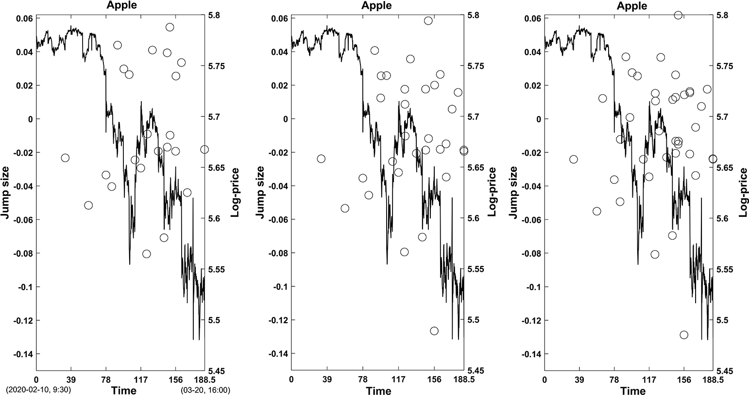
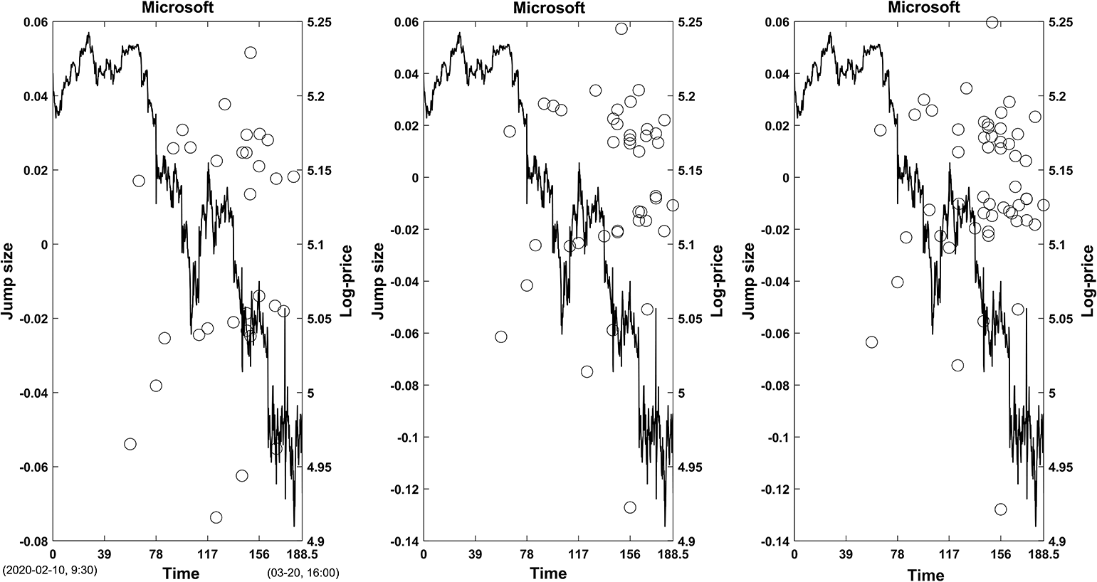
We evaluate the finite sample performance of the proposed test via Monte Carlo simulations. We also apply our test to the intraday price data of Apple and Microsoft stocks, and the results suggest relatively intensive jump arrivals during the market turbulent time of the year 2020.
The rest of this article is organized as follows. Section 2 introduces the model and assumptions. Section 3 describes the construction of the proposed test and develops the asymptotic theories. Section 4 theoretically extends the test to conditions where jumps have IA, or T grows to infinity jointly with
 $n.$
Section 5 carries out simulation studies, and Section 6 applies the test to stock price data of Apple and Microsoft. Section 7 concludes the article. The proof of the theorem, which reveals the global property of the randomized statistics unaffected by jumps for the case of fixed T and FA jumps, is given in the Appendix. The Supplementary Material contains some additional theoretical and numerical results, as well as proofs of the technical lemmas and corollaries.
2 FRAMEWORK
We use
 $x_t$
to denote the efficient log-price of some asset at time
 $t,$
and the dynamics of x are assumed to be driven by the drift–diffusion–jump model; that is,
 $$ \begin{align} x_t=x_0+\int_0^ta_sds+\int_0^t\sigma_sdB_s+J_t, \ \ t\in [0, T], \end{align} $$
where
 $B_t$
is a standard Brownian motion, and
 $a_t, \sigma _t$
, and
 $J_t$
are càdlàg processes, while
 $J_t$
is the component that generates jumps on the path of the efficient price with
 $J_0=0. a_t, \sigma _t, B_t$
, and
 $J_t$
are defined on a filtered probability space
 $(\Omega , \mathcal F, (\mathcal F_t)_{t\in [0,T]}, \mathrm {P}),$
and the filtration
 $\mathcal F_t\subseteq \mathcal F$
is
 $\mathrm {P}$
-complete and right-continuous.
As our test aims to identify the presence of jumps, the null and alternative hypotheses are given by
 $$ \begin{align*}H_0: \Delta J_t=0 \ \text{ for all } \ t\in(0, T), \ \ \text{ and } \ \ H_1: \Delta J_{\tau}\neq 0 \ \text{ for some } \ \tau\in(0, T),\end{align*} $$
for the context of a fixed
 $T,$
where
 $\Delta J_t=J_t-J_{t-}$
is the jump size of J at time t with
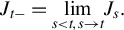 $J_{t-}=\underset {s<t, s\rightarrow t}{\lim } J_s.$
The observed prices are obtained at time grids
 $\left \{0=t_0<t_1<\cdots <t_n\right \}$
with
 $t_n\leq T,$
and
 $y_{t_i},$
the log-price observation at time
 $t_i,$
is given by
 $$ \begin{align*}y_{t_i}=x_{t_i}+u_{t_i},\end{align*} $$
where
 $u_{t_i}$
represents the noise at time
 $t_i.$
From now on, we use
 $x_i, y_i$
, and
 $u_i$
to, respectively, denote
 $x_{t_i}, y_{t_i}$
, and
 $u_{t_i}$
for notational simplicity. Our asymptotic results will be presented in the setting where
 $n\rightarrow \infty ,$
and we make the following assumptions to state regularity conditions needed for our theoretical analysis.
Assumption 1.
 $a_t$
and
 $\sigma _t$
are locally bounded processes.
Assumption 2. The value of T is fixed.
Assumption 3. There exists a constant
 $b_0,$
such that
 $t_{i+1}-t_{i}<b_0n^{-1}$
for any
 $i\in \{0,\ldots , n\},$
where
 $t_{n+1}=T$
and the time grids
 $\{t_1, \ldots , t_{n}\}$
are independent of
 $\mathcal F_T$
and the noise
 $\{u_i\}.$
Assumption 4.
 $\{u_i\}$
is independent of
 $\mathcal F_T$
and is an M-dependent time series for some constant
 $M>0. \mathbb {E}(u_i)=0,$
and
 $\mathbb {E}(u_i^2)<b_1$
for all i and some constant
 $b_1.$
Assumption 5.
 $J_t$
is an FA pure jump process.
Assumptions 1 and 2 are common in the literature on high-frequency econometrics, while we will consider the condition where T goes to infinity jointly with n in Section 4.2. Assumption 3 states that the time distance between any two adjacent observations is uniformly
 $O\left (n^{-1}\right ),$
which is more general than the standard assumption in the literature that requires observations to be equally spaced. Assumption 4 imposes mild regularity conditions on the noise terms that are allowed to be heteroskedastic in distribution and have some serial dependence. As mentioned before, theoretically we do not need to estimate the volatilities for jump detection, and this advantage can substantially save the technical restrictions, like the i.i.d. condition and the existence of a higher moment for the noise. Assumption 5, which assumes FA jumps, is commonly employed by literature on sequential jump testing (e.g., Lee and Mykland, Reference Lee and Mykland2008, Reference Lee and Mykland2012; Laurent and Shi, Reference Laurent and Shi2020). Under this assumption, the process
 $J_t$
almost surely has only a finite number of jumps on each finite interval, and thus when the alternative hypothesis
 $H_1$
holds,
 $J_t$
can be expressed as
 $$ \begin{align} J_t=\left\{\begin{aligned} & 0, \ \ 0<t<\tau_1, \\ & \sum_{i=1}^{N_t}\Delta J_{\tau_i}, \ \ \tau_1\leq t\leq T, \\ \end{aligned}\right. \end{align} $$
where starting from
 $N_0=0, N_t$
is a càdlàg counting process recording the number of jumps up to time
 $t, \tau _i$
is the arrival time of the ith jump, and
 $\Delta J_{\tau _i},$
which is nonzero for each
 $i,$
represents the size of the ith jump. In Section 4.1, we will relax Assumption 5 by allowing
 $J_t$
to have IA of jumps. Moreover, in our test, the significance level
 $\alpha $
has statistical implications even when
 $H_1$
holds. As the proposed procedure can be regarded as a global jump test consisting of many local tests, in the context of FA jumps, we aim to let the limiting probability of the family-wise type I error committed by tests associated with intervals that do not contain a jump tend to
 $\alpha ,$
which is in line with the principle of jump tests derived by Lee and Mykland (Reference Lee and Mykland2008, Reference Lee and Mykland2012).
3 METHODOLOGY
3.1 Robust LAR
Analogous to the practice of sequential jump tests in the literature (e.g., Lee and Mykland, Reference Lee and Mykland2008, Reference Lee and Mykland2012; Laurent and Shi, Reference Laurent and Shi2020), we test for jumps, respectively, over time windows whose lengths shrink as n grows, and the union of these windows basically covers
 $(0, T)$
for large
 $n.$
Specifically, the ith window is
 $\left [t_{(i-1)K_1}, t_{(i+1)K_1}\right ]$
with
 $i\in \mathcal {S}\!:=\left \{1, \dots , \lfloor (n-1)/K_1-1\rfloor \right \},$
where
 $\lfloor x\rfloor $
is the largest integer not larger than
 $x, K_1=\lfloor cn^{c_1}\rfloor $
for some constant
 $c_1\!\in \!(0, 1),$
and c is a generic positive constant which may take different values at different appearances throughout this article. For each
 $i\in \mathcal S,$
we compute the robust LAR
 $\bar {\phi }_i$
based on observations within the ith window, where
 $$ \begin{align*} \bar{\phi}_i=\arg\hspace{1mm}\underset{\phi\in\mathbb{R}}{\min}\sum_{j=0}^{K_1}\ell_{\beta_0}\left(y_{iK_1+j}-y_{(i-1)K_1+j}-\phi\right), \end{align*} $$
 $\beta _0=cn^{\bar {c}_0}$
for some constant
 $\bar {c}_0\!\in \!(0, c_1),$
and
 $$ \begin{align} \ell_{\beta_0}(y)=\begin{cases} 2\beta_0|y|-\beta_0^2, & \text{ if } |y|>\beta_0, \\ y^2, & \text{ if } |y|\leq \beta_0. \end{cases} \end{align} $$
Here,
 $\ell _{\beta _0}(\cdot )$
is the Huber loss function (Huber, Reference Huber1964) and recently has been widely used in the literature for the construction of statistics robust to fat-tailed noises (e.g., Fan et al., Reference Fan, Li and Wang2017; Fan and Kim, Reference Fan and Kim2018; Fan, Guo, and Jiang, Reference Fan, Guo and Jiang2022). When
 $\ell _{\beta _0}(y)$
is simply chosen as
 $y^2, \bar {\phi }_i$
would equal the LAR
 $\phi _i$
given by
 $$ \begin{align*}\phi_i=\sum_{j=0}^{K_1}(y_{iK_1+j}-y_{(i-1)K_1+j})/(K_1+1).\end{align*} $$
For a generic
 $i,$
the impact of the noise on
 $\phi _i$
vanishes in probability as n increases. However, in this article, we need to show that the maximum impact of the noise on the (robust) LAR for all the windows is negligible. Lee and Mykland (Reference Lee and Mykland2012) deal with such a problem under the assumption that the noise process is stationary in distribution, but in reality,
 $u_i$
’s can be heteroskedastic (see, e.g., the discussions in Kalnina, Reference Kalnina2011 and Taniai et al., Reference Taniai, Usami, Suto and Taniguchi2012). Then, following Sun (Reference Sun2024), we adopt the robust LAR
 $\bar {\phi }_i$
to build the local statistics for jump tests.
Compared to the choice of
 $\beta _0 :=\infty $
(which makes
 $\ell _{\beta _0}(y)=y^2$
as defined in (3.1)), employing a finite
 $\beta _0$
can relieve the impact of outliers in the noise on
 $\bar {\phi }_i$
’s, as
 $2\beta _0|y|-\beta _0^2\leq y^2,$
and noise outliers can induce abnormally large values in the absolute intraday returns
 $\left |y_{iK_1+j}-y_{(i-1)K_1+j}\right |.$
On the other hand,
 $\beta _0$
needs to be sufficiently large for us to control the bias in approximating the efficient LAR (i.e., the LAR of the efficient price) with
 $\bar {\phi }_i.$
Then choosing
 $\beta _0$
as a quantity growing jointly with n helps us to show the theoretical validity of
 $\bar {\phi }_i$
in approximating the efficient LAR uniformly across i in the presence of possibly fat-tailed noises.
Conditional on values of
 $\beta _0$
and observed prices, we define the functions
 $\bar {\ell }_i(\phi )=\sum _{j=0}^{K_1}\ell _{\beta _0}(y_{iK_1+j}-y_{(i-1)K_1+j}-\phi )$
and
 $$ \begin{align*}\tilde{\ell}_i(\phi)=\partial\bar{\ell}_i(\phi)/\partial\phi=-2\beta_0\sum_{j=0}^{K_1}f\left(\beta_0^{-1}\left(y_{iK_1+j}-y_{(i-1)K_1+j}-\phi\right)\right)\end{align*} $$
for
 $f(x)=\text { sign }(x)\min \left (\left |x\right |, 1\right )$
and
 $\phi \in \mathbb {R}.$
Notice that
 $\tilde {\ell }_i\left (\phi \right )\tilde {\ell }_i\left (-\phi \right )<0$
when
 $\left |\phi \right |$
is sufficiently large. Then there exists a solution to the equation
 $\tilde {\ell }_i(\phi )=0,$
since
 $\tilde {\ell }_i(\phi )$
is a continuous function. As
 $\bar {\ell }_i(\phi )$
is convex,
 $\tilde {\ell }_i(\bar {\phi }_i)=0$
according to the first-order condition. By Lemma S1 in the Supplementary Material, we show that the solution to the equation
 $\tilde {\ell }_i(\phi )=0$
is unique when
 $K_1$
is an even integer. Then we assume that
 $K_1$
is even to guarantee that
 $\bar {\phi }_i$
is well defined for theoretical analysis. Since minimizing
 $\bar {\ell }_i(\phi )$
belongs to the type of optimization problems considered by Qin and Fang (Reference Qin and Fang2023, Expression (2)), the value of
 $\bar {\phi }_i$
can be obtained with the iteratively reweighted least-squares (IRLS) approach as specified in that work.
Sun (Reference Sun2024) requires the noise terms to be mutually independent and variance-stationary in demonstrating the similarity between the robust LAR and the LAR of the efficient price, while we allow
 $u_i$
’s to be M-dependent and have time-varying variances. Then with more general regularity conditions on the noise, we show the property of the robust LAR in Lemma 1, which is analogous to Theorem 1 in Sun (Reference Sun2024) and is proved with techniques used in that work.
Lemma 1. Under Assumptions 1–5, for any fixed
 $\epsilon>0,$
we have
 $$ \begin{align} \underset{i\in\mathcal S}{\max} \ \left|\bar{\phi}_i-\sum_{j=0}^{K_1}(x_{iK_1+j}-x_{(i-1)K_1+j})/(K_1+1)\right|=O_{\mathrm{P}}\left(n^{\max(-\bar{c}_0, \bar{c}_0-c_1)+\epsilon}\right). \end{align} $$
Since the continuous increments of the efficient price are small within short intervals, Lemma 1 implies that for large
 $n, \left |\bar {\phi }_i\right |$
is small in probability when there is no jump on
 $\left (t_{(i-1)K_1}, t_{(i+1)K_1}\right ],$
which is the intuition of Equation (3.3) in Corollary 1 below. Notice that under the alternative hypothesis
 $H_1$
and Assumptions 2, 3, and 5, for
 $\mathrm {P}$
-almost all
 $\omega ,$
there exists some
 $n^*(\omega ),$
such that when
 $n>n^*(\omega )$
,
 $t_{K_1}(\omega )$
is smaller than the arrival time of the first jump on
 $(0, T)$
(i.e.,
 $\tau _1(\omega )>t_{K_1}(\omega )),$
since
 $t_{K_1}(\omega )$
tends to zero as n grows. The similar reasoning yields that as
 $n\rightarrow \infty ,$
there is almost surely no jump on
 $(t_{n-K_1}, T),$
and thus
 $\left [t_{K_1}, t_{n-K_1}\right ]$
almost surely contains all jumps on
 $(0, T).$
On the other hand, any jump on
 $\left [t_{K_1}, t_{n-K_1}\right ]$
is contained in two consecutive intervals in the form of
 $\left [t_{(i-1)K_1}, t_{(i+1)K_1}\right ]$
for
 $i\in \mathcal S$
(see Figure 1). Thus, a jump on
 $(0, T)$
can affect the values of two
 $\bar {\phi }_i$
’s, and Corollary 1 implies that with high probability, it significantly increases the absolute value of at least one
 $\bar {\phi }_i.$
This figure shows that for a jump which occurs at time
 $t_{iK_1}+\triangle t$
with
 $0\leq \triangle t\leq t_{(i+1)K_1}-t_{iK_1},$
it is contained in both blocks
 $\left [t_{(i-1)K_1}, t_{(i+1)K_1}\right ]$
and
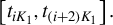 $\left [t_{iK_1}, t_{(i+2)K_1}\right ].$

Corollary 1.
(a) Define
 $\mathcal S_0=\Big \{\ell : \ell \in \mathcal S, \ \text { and } \ \Delta J_t=0 \ \text { for all } \ t\in (t_{(\ell -1)K_1}, t_{(\ell +1)K_1}]\Big \}$
and
 $\tilde {c}_0=\min (\bar {c}_0, c_1-\bar {c}_0, (1-c_1)/2).$
Then, for any fixed
 $\epsilon>0,$
under Assumptions 1–5, we have
 $$ \begin{align} \underset{i\in\mathcal S_0}{\max} \ \left|\bar{\phi}_i\right|=O_{\mathrm{P}}\left(n^{-\tilde{c}_0+\epsilon}\right). \end{align} $$
(b) Suppose that Assumptions 2, 3, and 5 hold. Then, for
 $\mathrm {P}$
-almost all
 $\omega ,$
there exists some
 $\bar {n}(\omega ),$
such that when
 $n>\bar {n}(\omega ),$
 $$ \begin{align*} \underset{i\in\mathcal S}{\max} \ (N_{t_{(i+1)K_1}}(\omega)-N_{t_{(i-1)K_1}}(\omega))\leq 1. \end{align*} $$
(c) Under Assumptions 1–5 and the alternative hypothesis
 $H_1,$
it holds that
 $$ \begin{align} \mathrm{P}\left(\underset{i\in\{1,\ldots , N_{T-}\}}{\cap} \ \left\{h_i\in\mathcal S, \ \text{ and } \ |\bar{\phi}_{h_i}|>\tilde{c}_1|\Delta J_{\tau_i}|\right\}\right)\overset{n\rightarrow\infty}{\longrightarrow} 1 \end{align} $$
for any constant
 $\tilde {c}_1<1/2,$
where
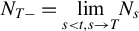 $N_{T-}=\underset {s<t, s\rightarrow T}{\lim } N_s$
and
 $h_i\in \left \{0,\dots , \text { card }(S)+1\right \}$
is defined such that
 $\tau _i\in \tilde {L}_i :=(t_{\lceil (h_i-1/2)K_1\rceil \vee 0}, t_{\lceil (h_i+1/2)K_1\rceil \wedge (n+1)}]$
for each
 $i\in \{1, \ldots , N_{T-}\},$
with
 $x\wedge y$
and
 $x\vee y,$
respectively, representing
 $\min (x,y)$
and
 $\max (x,y),$
and
 $\lceil x\rceil $
being the smallest integer not smaller than
 $x.$
Corollary 1(a) indicates that the absolute values of the
 $\bar {\phi }_i$
’s unaffected by jumps are small in probability for large
 $n.$
Corollary 1(b) says that there is almost surely at most one jump on
 $(t_{(i-1)K_1}, t_{(i+1)K_1}]$
for each
 $i\in \mathcal S$
as
 $n\rightarrow \infty .$
Corollary 1(c) suggests that under
 $H_1,$
with high probability, there exists a
 $\bar {\phi }_{h_i}$
for each
 $i\in \{1,\ldots , N_{T-}\},$
such that the absolute value of
 $\bar {\phi }_i$
is substantially enlarged by the ith jump on
 $(0, T).$
Notice that
 $h_i\in \mathcal S$
for each
 $i\in \{1, \ldots , N_{T-}\},$
when there is no jump on
 $(0, t_{K_1})\cup (t_{n-K_1}, T).$
Then the discussion above Corollary 1 indicates that the event
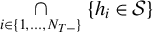 $\underset {i\in \{1,\ldots , N_{T-}\}}{\cap } \ \{h_i\in \mathcal S\}$
holds almost surely as
 $n\rightarrow \infty .$
In proving Corollary 1(c), we show that the jump size
 $\Delta J_{\tau _i}$
is likely to be dominating in determining the value of
 $\bar {\phi }_{h_i},$
since the impact of the continuous component in the price on
 $\bar {\phi }_i$
is vanishing in probability as
 $n\rightarrow \infty .$
Given Lemma 1 which reveals the similarity between the robust LAR and the LAR of the efficient price, the contribution by the ith jump to
 $\bar {\phi }_{h_i}$
can be roughly expressed as
 $\psi _i\Delta J_{\tau _i},$
and the value of
 $\psi _i$
is dependent on
 $\tau _i$
and the (left and right) boundaries of the time window
 $\tilde {L}_i.$
We let
 $\tilde {c}_1$
in (3.4) be smaller than
 $1/2,$
since
 $1/2$
is the infimum of
 $\psi _i$
as
 $\tau _i$
varies within
 $\tilde {L}_i$
and
 $n\rightarrow \infty .$
The essential reason is that as
 $\tau _i\in \tilde {L}_i,$
numbers of price observations on intervals
 $[t_{(h_i-1)K_1}, \tau _i] $
and
 $[\tau _i, t_{(h_i+1)K_1}]$
are both not smaller than
 $\lfloor K_1/2\rfloor -1$
conditional on
 $h_i\in \mathcal S.$
In contrast, if we consider non-overlapping intervals over which we test for jumps, respectively, with the current assumptions, we cannot roughly exclude the possibility that there are not many price observations between the arrival time of a jump and the left/right boundary of the time window that contains this jump. Then with non-overlapping windows, it would be more difficult to demonstrate that a jump is likely to exert significant impact on some robust LAR. Moreover, in the literature, it is typical to consider overlapping time windows for sequential jump tests constructed with noisy data (e.g., Lee and Mykland, Reference Lee and Mykland2012; Sun, Reference Sun2019, Reference Sun2024).
3.2 Randomized Tests
Given Corollary 1, we can utilize differences in the magnitudes of
 $\bar {\phi }_i$
’s to detect jumps with randomized tests. As mentioned before, the significance level of this test is defined as the limiting probability of the GTE, which means that there exists some
 $i\in \mathcal S_0,$
such that we mistakenly believe that there is a jump on
 $(t_{(i-1)K_1}, t_{(i+1)K_1}]$
due to the test result. In addition to controlling the significance level, we aim to let the likelihood of missing any jump on
 $(0, T)$
vanish as
 $n\rightarrow \infty .$
Then we propose procedures as follows to obtain the randomized statistics
 $\eta _i$
across
 $i\in \mathcal S$
:
-
1. Define
 $\bar {g}_n=cn^{-\tilde {c}_2}$
for some constant
$\tilde {c}_2\in (0,\tilde {c}_0).$
Compute
$\bar {\eta }_i=\exp \left (-\left |\bar {g}_n/\bar {\phi }_i\right |\right )$
for
$i\in \mathcal S.$
-
2. For each
$i\in \mathcal S,$
independently generate
$L_n$
i.i.d. random variables
$\left \{z_{i,j}\right \}_{j=1}^{L_n},$
with
$z_{i, j}\sim \mathcal D$
for some distribution
$\mathcal D$
and
$L_n=cn^{c_2}$
for some positive constant
$c_2>2(1-c_1).$
-
3. For each
$i\in \mathcal S,$
compute (3.5)
$$ \begin{align} \eta_i :=2L_n^{-1/2}\sum_{j=1}^{L_n}\left(\boldsymbol 1_{\left\{\bar{\eta}_i\geq z_{i,j}\right\}}-2^{-1}\right). \end{align} $$








We denote the CDF of
 $\mathcal D$
as
 $\tilde {F}(\cdot ),$
and state regularity conditions concerning
 $\tilde {F}(\cdot )$
in Assumption 6, which is satisfied when
 $\mathcal D$
is, for example, the centered uniform or Gaussian distribution.
Assumption 6.
 $\tilde {F}(\cdot )$
satisfies the following conditions: (a)
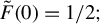 $\tilde {F}(0)=1/2;$
(b) there exist some
 $\tilde {b}_0>0$
and
 $\tilde {b}_1>0,$
such that
 $\tilde {F}(x)$
is differentiable and
 $\partial \tilde {F}(x)/\partial x<\tilde {b}_1$
for
 $x\in [0, \tilde {b}_0]; $
and
(c)
 $\tilde {F}(1-\tilde {b}_2)-1/2>0$
for some
 $\tilde {b}_2>0.$
For
 $i\in \mathcal S,$
we believe that there is a jump (or no jump) on
 $(t_{(i-1)K_1}, t_{(i+1)K_1}]$
if
 $\eta _i$
is larger (or smaller) than the test threshold
 $\mathcal T_n.$
Then the GTE refers to the event that
 $\underset {i\in \mathcal S_0}{\max } \ \eta _i$
is larger than
 $\mathcal T_n,$
and thus knowledge on the asymptotic behavior of
 $\underset {i\in \mathcal S_0}{\max } \ \eta _i$
is needed in order to set the value of
 $\mathcal T_n$
given the prescribed significance level. On the other hand, Corollary 1(a) indicates that in the absence of jumps, with high probability
 $\bar {\eta }_i$
’s are uniformly small, which implies that whether
 $\bar {\eta }_i$
is larger than
 $z_{i, j}$
is basically determined by the sign of
 $z_{i,j}.$
Consequently, the difference between
 $\eta _i$
and
 $\tilde {\eta }_i$
is vanishing in probability uniformly for all
 $i\in \mathcal S_0,$
where
 $$ \begin{align*}\tilde{\eta}_i=2L_n^{-1/2}\sum_{j=1}^{L_n}\left(\boldsymbol 1_{\left\{0\geq z_{i,j}\right\}}-2^{-1}\right),\end{align*} $$
which is asymptotically standard Gaussian by the central limit theorem. The methodology developed by Galambos (Reference Galambos1978) indicates that the asymptotic distribution of the maximum among many i.i.d. random variables can be derived based on the tail behavior of the CDF of a generic individual variable. Then we investigate the asymptotic distribution of
 $\underset {i\in \mathcal S_0}{\max } \ \eta _i$
based on the derived similarity between the tail probabilities of
 $\tilde {\eta }_i$
and the standard Gaussian variable, and the similarity between
 $\eta _i$
and
 $\tilde {\eta }_i.$
In particular, we utilize the characteristic function to study the tail probability of
 $\tilde {\eta }_i$
in the technical proofs. Now, we describe the asymptotic behavior of
 $\underset {i\in \mathcal S_0}{\max } \ \eta _i$
in Theorem 1, which indicates that
 $\underset {i\in \mathcal S_0}{\max } \ \eta _i$
has the same asymptotic distribution as the maximum of
 $\lfloor n/K_1 \rfloor $
independent standard Gaussian variables (see, e.g., Chapter 2 in Galambos, Reference Galambos1978).
Theorem 1. Under Assumptions 1–5, for any fixed
 $\bar {x}\in \mathbb R,$
we have
 $$ \begin{align*}\mathrm{P}\left(\underset{i\in\mathcal S_0}{\max} \ \left(\eta_i-\bar{a}_n\right)/\bar{b}_n\leq\bar{x}\right)\rightarrow \exp\left(-e^{-\bar{x}}\right),\end{align*} $$
as
 $n\rightarrow \infty ,$
where
 $$ \begin{align*}\bar{a}_n=\left(2\ln\left(n/K_1\right)\right)^{1/2}-\frac{2^{-1}\left(\ln\left(\ln\left(n/K_1\right)\right)+\ln(4\pi)\right)}{\left(2\ln\left(n/K_1\right)\right)^{1/2}},\end{align*} $$
and
 $\bar {b}_n=\left (2\ln (n/K_1)\right )^{-1/2}.$
Theorem 1 suggests that given the significance level
 $\alpha>0,$
we can set the test threshold
 $\mathcal T_n$
as
 $$ \begin{align} \mathcal T_n :=\bar{a}_n-\bar{b}_n\ln\left(-\ln(1-\alpha)\right), \end{align} $$
so that
 $$ \begin{align*}\mathrm{P}\left(\underset{i\in\mathcal S_0}{\max} \ \eta_i>\mathcal T_n\right)\overset{n\rightarrow\infty}{\longrightarrow}\alpha.\end{align*} $$
On the other hand, detecting a given jump with our test means that there exists some
 $i\in \mathcal S,$
such that the arrival time of this jump falls on
 $(t_{(i-1)K_1}, t_{(i+1)K_1}]$
and
 $\eta _i>\mathcal T_n.$
Corollary 2 below suggests that each jump on
 $(0, T)$
is likely to cause one
 $\eta _i$
associated with a window containing this jump to be at the order of
 $n^{c_2/2}.$
Then since
 $\mathcal T_n$
is at the order of
 $\sqrt {\ln (n)}$
under (3.6), based on the comparison between
 $\eta _i$
’s and
 $\mathcal T_n$
, we can let the limiting probability of the GTE tend to
 $\alpha ,$
and detect all jumps on
 $(0, T)$
with probability tending to one as
 $n\rightarrow \infty .$
Corollary 2. Recall the definition of
 $h_i$
in Corollary 1. Under Assumptions 1–5 and the alternative hypothesis
 $H_1,$
there exists some positive constant
 $c,$
such that
 $$ \begin{align*}\mathrm{P}\left(\underset{i\in\{1,\ldots , N_{T-}\}}{\min} \ \eta_{h_i}>cn^{c_2/2}\right)\overset{n\rightarrow\infty}{\longrightarrow}1.\end{align*} $$
Moreover, we can conveniently construct a randomized test to examine whether there is a jump at one or multiple given time points. The corresponding test and the associated theories are presented in Section 1 in the Supplementary Material.
With a mild abuse of notation, an alternative choice of
 $\bar {\eta }_i$
is to let
 $\bar {\eta }_i=\left |\bar {\phi }_i/\bar {g}_n\right |$
in computing the randomized statistics
 $\eta _i,$
in which case it still holds that
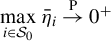 $\underset {i\in \mathcal S_0}{\max } \ \bar {\eta }_i\overset {\mathrm {P}}{\rightarrow } 0^+$
as
 $n\rightarrow \infty $
by Corollary 1(a). However, as
 $\exp \left (-x^{-1}\right )/x\overset {x\rightarrow 0^+}{\longrightarrow } 0^+,$
the exponential transformation that we adopt in Step 1 of the randomization procedures can substantially decrease values of
 $\bar {\eta }_i$
for
 $i\in \mathcal S_0,$
compared to the choice of
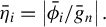 $\bar {\eta }_i=\left |\bar {\phi }_i/\bar {g}_n\right |.$
Then, with high probability, the exponential transformation would make
 $\eta _i$
more similar to
 $\tilde {\eta }_i$
for
 $i\in \mathcal S_0,$
which facilitates the derivation of the asymptotic distribution of
 $\underset {i\in \mathcal S_0}{\max } \ \eta _i.$
Moreover, in constructing randomized tests, it is a common practice to apply the exponential transformation to the original statistics (see, e.g., Trapani, Reference Trapani2018; Barigozzi and Trapani, Reference Barigozzi and Trapani2022; Sun, Xu, and Zhang, Reference Sun, Xu and Zhang2023).
Alternatively, we may also choose
 $\bar {\eta }_i$
as
 $$ \begin{align*} \bar{\eta}_i=\exp\left(\left|\bar{g}_n/\bar{\phi}_i\right|\right), \end{align*} $$
in which case
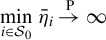 $\underset {i\in \mathcal S_0}{\min } \ \bar {\eta }_i\overset {\mathrm {P}}{\rightarrow } \infty $
as
 $n\rightarrow \infty $
by Corollary 1(a), and accordingly, the final statistic
 $\eta _i$
can be redefined as
 $$ \begin{align} \eta_i :=\int_U\left(2L_n^{-1/2}\sum_{j=1}^{L_n}\left(\boldsymbol 1_{\left\{\bar{\eta}_iz_{i,j}\leq |u|\right\}}-1/2\right)\right)^2 dF(u) \end{align} $$
for
 $i\in \mathcal S,$
where U and
 $F(u)$
are, respectively, the support and CDF of some chosen distribution. Actually, the statistics (after the exponential transformation) to which the randomization technique is applied in Trapani (Reference Trapani2018), Barigozzi and Trapani (Reference Barigozzi and Trapani2022), and Sun et al. (Reference Sun, Xu and Zhang2023) tend to infinity in probability under the null hypothesis, and their randomized statistics are constructed in similar fashion as shown in (3.7). Given Corollary 1(a), it is straightforward to verify that under certain regularity conditions,
 $\eta _i$
given by (3.7) is asymptotically subject to the distribution of
 $\chi _1^2$
for each
 $i\in \mathcal S_0$
as
 $n\rightarrow \infty .$
However, we employ the randomized statistic given by (3.5) rather than the one defined in (3.7) to build the test, since in this way, we do not need to choose the distribution characterized by U and
 $F(u).$
From now on, we stick to the choices of
 $\bar {\eta }_i=\exp \left (-\left |\bar {g}_n/\bar {\phi }_i\right |\right )$
and
 $\eta _i$
given by (3.5). When Assumption 6(a) is changed to the weaker assumption that
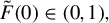 $\tilde {F}(0)\in (0, 1),$
Corollary 1(a) suggests that under certain regularity conditions (including Assumption 6), the statistic
 $$ \begin{align*}\sum_{j=1}^{L_n}\left(\boldsymbol 1_{\left\{\bar{\eta}_i\geq z_{i,j}\right\}}-\tilde{F}(0)\right)/\sqrt{L_n\tilde{F}(0)\left(1-\tilde{F}(0)\right)}\end{align*} $$
is asymptotically standard Gaussian for
 $i\in \mathcal S_0.$
However, we need the condition that
 $\tilde {F}(0)=1/2$
(as assumed in Assumption 6(a)) for analyzing the tail probabilities of
 $\tilde {\eta }_i$
’s (or
 $\eta _i$
’s for
 $i\in \mathcal S_0$
) in the technical proofs.
3.3 Inferences on the Number and Sizes of Jumps
As a jump on
 $(0, T)$
can be contained in two consecutive intervals in the form of
 $\left [t_{(i-1)K_1}, t_{(i+1)K_1}\right ]$
for
 $i\in \mathcal S,$
we can overestimate the number of jumps if we record the number of all the
 $\eta _i$
’s that are larger than
 $\mathcal T_n$
as the estimator. If both
 $\eta _i$
and
 $\eta _{i+1}$
are larger than the threshold, under Assumptions 2, 3, and 5, it is likely to be the same jump on
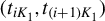 $(t_{iK_1}, t_{(i+1)K_1})$
that increases the values of these two statistics, since, with high probability, there is at most one jump on
 $[t_{(i-1)K_1}, t_{(i+2)K_1}]$
for large
 $n.$
Accordingly, we propose the estimator for the number of jumps on
 $(0, T)$
as
 $\hat {N}=\text { card }(\mathcal S_1),$
where
 $$ \begin{align*}\mathcal S_1=\left\{i: i\in\mathcal S, i>1, \eta_{i-1}\leq\mathcal T_n, \text{ and } \ \eta_{i}>\mathcal T_n\right\}.\end{align*} $$
When the threshold
 $\mathcal T_n$
is given by (3.6), Theorem 1 indicates that the limiting probability of the GTE tends to
 $\alpha \in (0, 1).$
Then it can only be shown that
 $\hat {N}$
equals
 $N_{T-}$
with probability approaching
 $1-\alpha $
instead of 1. However, if
 $\mathcal T_n$
is redefined such that
 $$ \begin{align} \mathcal T_n/\sqrt{\ln(n)}\rightarrow\infty, \ \text{ and } \ \mathcal T_n/n^{c_2/2}\rightarrow 0 \end{align} $$
as
 $n\rightarrow \infty ,$
which holds when, for example,
 $\mathcal T_n=cn^{\tilde {b}_3}$
for some constant
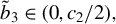 $\tilde {b}_3\in (0, c_2/2),$
given Theorem 1 and Corollary 2, it is straightforward to verify that
 $\hat {N}$
converges to
 $N_{T-}$
in probability, since the probability of committing the GTE or missing any jump on
 $(0, T)$
tends to zero. Now, we state these results in Corollary 3.
Corollary 3. In the setting of Theorem 1, it holds that:
(a)
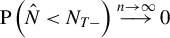 $\mathrm {P}\left (\hat {N}<N_{T-}\right )\overset {n\rightarrow \infty }{\longrightarrow } 0$
and
 $\mathrm {P}\left (\hat {N}=N_{T-}\right )\overset {n\rightarrow \infty }{\longrightarrow } 1-\alpha $
under (3.6);
(b)
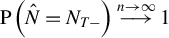 $\mathrm {P}\left (\hat {N}=N_{T-}\right )\overset {n\rightarrow \infty }{\longrightarrow } 1$
under (3.8).
Theorem 1 and Corollary 2 suggest that when (3.8) holds, with probability approaching one, the proposed method can identify all jumps on
 $(0, T)$
without committing the GTE. However, in line with the literature on sequential jump tests (e.g., Lee and Mykland, Reference Lee and Mykland2008, Reference Lee and Mykland2012; Laurent and Shi, Reference Laurent and Shi2020), we aim to let the probability of the GTE converge to some prescribed significance level
 $\alpha \in (0, 1),$
and thus assume that
 $\mathcal T_n$
is given by (3.6) in the remainder of this article.
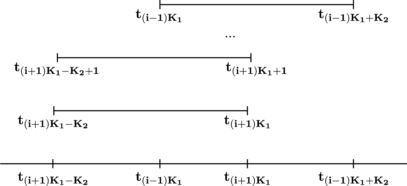
Figure 2 indicates that when
 $K_2\geq 2K_1, (i+1)K_1-K_2\geq 0,$
and
 $(i-1)K_1+K_2\leq n$
with
 $K_2\in \mathbb {N}^+,$
an interval
 $[t_{(i-1)K_1}, t_{(i+1)K_1}]$
is contained in
 $K_2-2K_1+1$
intervals in the form of
 $[t_\ell , t_{\ell +K_2}]$
for
 $\ell \in \{(i+1)K_1-K_2,\ldots , (i-1)K_1\}.$
Then when the test detects a jump on
 $[t_{(i-1)K_1}, t_{(i+1)K_1}],$
we can use the LAR
 $\bar {y}_i$
given by
 $$ \begin{align*}\bar{y}_i=\sum_{k=0}^{K_2-2K_1}\left(y_{((i+1)K_1+k)\wedge n}-y_{((i+1)K_1+k-K_2)\vee 0}\right)/(K_2-2K_1+1)\end{align*} $$
to estimate the jump size, where
 $K_2-2K_1=cn^{c_3}$
for some constant
 $c_3\in [c_1, 1).$
Since the length of an interval
 $[t_\ell , t_{\ell +K_2}]$
is
 $O\left (n^{c_3-1}\right )$
by Assumptions 2 and 3, the contribution to
 $\bar {y}_i$
from the continuous component in the price can be bounded at a small level in probability uniformly for all
 $i\in \mathcal S.$
In addition, for a generic i with
 $ (i+1)K_1-K_2\geq 0$
and
 $(i-1)K_1+K_2\leq n,$
the effect of the noise on
 $\bar {y}_i$
can be roughly smoothed away by the averaging scheme. Then since the occurrence of jumps is independent of the noise,
 $\bar {y}_i$
is a consistent jump size estimator for each
 $i\in \mathcal S_2$
under the alternative hypothesis
 $H_1,$
where
 $\mathcal S_2=\left \{i:i\in \mathcal S, \ \text { and } \ N_{t_{(i+1)K_1}}-N_{t_{(i-1)K_1}}>0\right \}.$
On the other hand, we can obtain reliable information about the jump arrival times from the test result, which facilitates the estimation of jump sizes with
 $\bar {y}_i.$
Now, we summarize these results in Corollary 4.
The figure shows that there are
 $K_2-2K_1+1$
intervals in the form of
 $[t_\ell , t_{\ell +K_2}]$
that contain the interval
 $[t_{(i-1)K_1}, t_{(i+1)K_1}].$

Corollary 4. Under the alternative hypothesis
 $H_1$
and Assumptions 1–5, it holds that:
 $$ \begin{align} \mathrm{P}\left(\hat{N}=N_{T-}, \ \text{ and } \ \ \underset{i\in\mathcal S_0}{\max} \ \eta_i\leq\mathcal T_n\right)\overset{n\rightarrow\infty}{\longrightarrow}1-\alpha, \ \ \text{ and } \end{align} $$
 $$ \begin{align} \underset{i\in\mathcal S_2}{\max} \ \left|\bar{y}_i-\sum_{\ell=1}^{N_{T-}}\Delta J_{\tau_\ell}\boldsymbol 1_{\left\{\tau_\ell\in (t_{(i-1)K_1}, t_{(i+1)K_1}]\right\}}\right|=O_{\mathrm{P}}\left(n^{-c_3/2}\vee \left(n^{(c_3-1)/2}\sqrt{\ln(n)}\right)\right). \end{align} $$
The convergence in (3.9) implies that when
 $\alpha $
is small, with high probability, the proposed test can locate the arrival time of each jump on
 $(0, T)$
within some interval in the form of
 $(t_{(i-1)K_1}, t_{(i+1)K_1}]$
without spurious jump detection, while (3.9) can be proved with steps that are essentially similar to those in the proof of Corollary 3(a). Equation (3.10) indicates that the difference between
 $\bar {y}_i$
and the jump size on
 $(t_{(i-1)K_1}, t_{(i+1)K_1}]$
can be bounded at a small level in probability for
 $i\in \mathcal S_2.$
4 EXTENSIONS
4.1 Asymptotic Results in the Presence of Infinite Activity Jumps
The previous analyses rely on the assumption that jumps only have FA. However, the empirical studies by, for example, Aït-Sahalia and Jacod (Reference Aït-Sahalia and Jacod2011, Reference Aït-Sahalia and Jacod2014), Jing et al. (Reference Jing, Kong, Liu and Mykland2012), Todorov (Reference Todorov2015), and Kong (Reference Kong2019) suggest the presence of IA jumps in financial markets. Accordingly, we extend our analyses to the condition where jumps may have IA in this section. Specifically, we suppose that
 $J_t$
is given by the sum of an FA jump process and a Lévy process that possibly has IA of jumps, as stated in Assumption 7.
Assumption 7. There exist an FA pure jump process
 $J_{t}^1$
and a Lévy process
 $J_{t}^2,$
which are adapted to
 $\mathcal F_t,$
such that
 $J_{t}=J_{t}^1+J_{t}^2$
for
 $t\in [0, T].$
The two processes
 $\left \{J_t^1\right \}$
and
 $\left \{J_t^2\right \}$
are independent, and
 $J_{t}^2$
is given by
 $$ \begin{align} J_t^2=\int_0^t\int_{|x|>1}x\mu(dx, ds)+\int_0^t\int_{|x|\leq 1}x(\mu(dx, ds)-\nu(dx)ds), \end{align} $$
where
 $\mu $
is a Poisson random measure on
 $[0, T]\times \mathbb {R}$
with intensity measure
 $\nu (dx)dt.$
Assumption 7 allows the process
 $J_t^2$
to have infinite number of jumps within a finite interval, and regularity conditions similar to this assumption have been widely employed in the literature to characterize jumps in asset prices (see, e.g., Mancini, Reference Mancini2009, Reference Mancini2017; Cont and Mancini, Reference Cont and Mancini2011; Sun et al., Reference Sun, Xu and Zhang2023; Shin, Kim, and Fan, Reference Shin, Kim and Fan2023). On the right-hand side of Equation (4.1), the component
 $\int _0^t\int _{|x|>1}x\mu (dx, ds),$
which is a compound Poisson process, is driven by jumps whose absolute sizes are larger than one, and
 $\int _0^t\int _{|x|\leq 1}x(\mu (dx, ds)-\nu (dx)ds)$
is the compensated sum of jumps with sizes not larger than one in absolute value, while
 $\tilde {\mu }(dx,ds):=\mu (dx, ds)-\nu (dx)ds$
is the compensated Poisson random measure associated with
 $\mu .$
Under Assumption 7 and some other regularity conditions, we can show that
 $\bar {\phi }_i$
is still valid in approximating the LAR of the efficient price, as indicated in Lemma 2.
Lemma 2. Under Assumptions 1–4 and 7, we have
 $$ \begin{align*}\underset{i\in\mathcal S}{\max} \ \left|\bar{\phi}_i-\sum_{j=0}^{K_1}(x_{iK_1+j}-x_{(i-1)K_1+j})/(K_1+1)\right|=O_{\mathrm{P}}\left(n^{\max(-\bar{c}_0, \bar{c}_0-c_1)+\epsilon}\right)\end{align*} $$
for any fixed
 $\epsilon>0.$
The convergence rate shown in Lemma 2 is the same as in Lemma 1, as
 $J_t^2$
does not substantially affect the robustness of
 $\bar {\phi }_i$
to the noise. Under Assumption 7, the magnitude of jump sizes that may cause the corresponding
 $\eta _i$
’s to be larger than
 $\mathcal T_n$
is related to the vibrancy of small jumps in
 $J_t^2,$
which can be measured by the
 $Blumenthal$
–
 $Getoor$
(BG) index defined as
 $$ \begin{align*}\tilde{\gamma} := \inf \ \left\{\gamma\geq 0, \int_{|x|\leq 1}|x|^\gamma\nu(dx)<\infty\right\}\leq 2.\end{align*} $$
The BG index has been widely considered in the literature (e.g., Todorov, Reference Todorov2017; Kong, Reference Kong2019; Park and Wang, Reference Park and Wang2021), and estimation methods for this index can be found in Aït-Sahalia and Jacod (Reference Aït-Sahalia and Jacod2009) and Jing et al. (Reference Jing, Kong, Liu and Mykland2012). A larger value of
 $\tilde {\gamma }$
suggests that small jumps in
 $J_t^2$
are more vibrant. In particular,
 $\tilde {\gamma }=0$
when
 $J_t^2$
is an FA jump process, and
 $\tilde {\gamma }\leq 1$
when
 $J_t^2$
is of finite variation. In expressing our theories, we treat
 $c/\tilde {\gamma }$
as infinity when
 $\tilde {\gamma }=0.$
Now, we use Corollary 5 to shed some light on asymptotic behaviors of some relevant statistics with Assumption 7.
Corollary 5.
(a) Suppose that Assumptions 2, 3, and 7 hold, and define
 $\bar {N}_{t,x} :=\sum _{s\in (0, t]}\boldsymbol 1_{\left \{\left |\Delta J_s\right |\geq x\right \}}.$
Then, for any fixed
 $\epsilon \in (0, (1-c_1)/(2\tilde {\gamma })),$
we have
 $$ \begin{align} \mathrm{P}\left(\underset{i\in\mathcal S}{\max} \ \left(\bar{N}_{t_{(i+1)K_1}, n^{-\epsilon}}-\bar{N}_{t_{(i-1)K_1}, n^{-\epsilon}}\right)\leq 1\right)\overset{n\rightarrow\infty}{\longrightarrow}1. \end{align} $$
(b) For any constants
 $\epsilon \in (0, \min ((1-c_1)/\max (2\tilde {\gamma }, 1+\tilde {\gamma }), \bar {c}_0, c_1-\bar {c}_0))$
and
 $\tilde {c}_1<1/2,$
under the alternative hypothesis
 $H_1$
and Assumptions 1–4 and 7, the event
 $$ \begin{align*} \left\{\bar{N}_{T-,n^{-\epsilon}}>0, \ \text{ and } \ \underset{i\in\{1,\ldots , \bar{N}_{T-,n^{-\epsilon}}\}}{\cap}\left\{\bar{h}_{i,n^{-\epsilon}}\in\mathcal S, \ \text{ and } \ |\bar{\phi}_{\bar{h}_i, n^{-\epsilon}}|>\tilde{c}_1|\Delta J_{\bar{\tau}_{i,n^{-\epsilon}}}|\right\}\right\} \end{align*} $$
holds with probability approaching 1 as
 $n\rightarrow \infty ,$
where
 $\bar {N}_{T-,x}=\underset {s<T, s\rightarrow T}{\lim } \bar {N}_{s,x},$
and
 $\bar {h}_{i,x}$
is defined such that
 $\bar {h}_{i, x}\in \{0, \dots , \text { card }(\mathcal S)+1\}$
and
 $\bar {\tau }_{i,x}\in (t_{\lceil (\bar {h}_{i,x}-1/2)K_1\rceil \vee 0}, t_{\lceil (\bar {h}_{i,x}+1/2)K_1\rceil \wedge (n+1)}]$
for each
 $i\in \{1, \ldots , \bar {N}_{T-,x}\},$
with
 $\bar {\tau }_{i,x}\in \left \{\tau : \tau \in (0, T), \ \text { and } \ |\Delta J_\tau |\geq x\right \}$
and
 $\bar {\tau }_{i,x}<\bar {\tau }_{j,x}$
if
 $i<j.$
(c) Suppose that Assumptions 1–4 and 7 hold. For any fixed
 $\epsilon \in (0, (1-c_1)/\tilde {\gamma })$
and
 $\tilde {\epsilon }>0,$
it follows that
 $$ \begin{align} \sum_{i\in\mathcal S}\boldsymbol 1_{\left\{\bar{N}_{t_{(i+1)K_1}, n^{-\epsilon}}-\bar{N}_{t_{(i-1)K_1}, n^{-\epsilon}}>0\right\}}=o_{\mathrm{P}}(n^{1-c_1}), \end{align} $$
and the event
 $$ \begin{align*} \underset{i\in\mathcal S}{\cap}\left\{\boldsymbol 1_{\left\{\bar{N}_{t_{(i+1)K_1}, n^{-\epsilon}}-\bar{N}_{t_{(i-1)K_1}, n^{-\epsilon}}>0\right\}}\geq\boldsymbol 1_{\left\{\left|(K_1+1)^{-1}\sum_{j=0}^{K_1}(J_{t_{iK_1+j}}-J_{t_{(i-1)K_1+j}})\right|\geq n^{(\tilde{\gamma}/2-1)\epsilon+\tilde{\epsilon}}\right\}}\right\} \end{align*} $$
holds with probability approaching 1 as
 $n\rightarrow \infty .$
Corollary 5(a) roughly suggests that with probability approaching one, each local window contains at most one jump whose size is at an order larger than
 $n^{(c_1-1)/(2\tilde {\gamma })}.$
Given Corollary 1(a) which shows the order of the robust LAR’s unaffected by jumps, Corollary 5(b) intuitively indicates that relatively large jumps, whose absolute sizes are bigger than some frequency-specific threshold, can substantially enlarge the corresponding robust LAR’s in absolute value, while (4.2) guarantees that each of these jumps affects a distinct robust LAR in probability. We prove Corollary 5(b) by verifying that a relatively large jump is likely to be dominating in determining the value of the corresponding robust LAR. Corollary 5(c) intuitively suggests that with high probability, most windows contain only small jumps, and for such windows, the impact of jumps on the associated robust LAR’s can be bounded at a small level when
 $\tilde {\gamma }<2,$
as Lemma 2 shows that the effects of jumps on
 $\bar {\phi }_i$
can be roughly expressed as
 $(K_1+1)^{-1}\sum _{j=0}^{K_1}(J_{t_{iK_1+j}}-J_{t_{(i-1)K_1+j}}).$
Lemma 2 and Corollary 5 imply that under certain regularity conditions including Assumption 7, with the proposed test, it is hopeful to detect relatively large jumps whose absolute sizes are allowed to decrease as n increases, since these jumps have substantially larger impact on the robust LAR than the continuous component and small jumps in the price. Moreover, in the presence of IA jumps, we can derive the extreme value theory in similar fashion as shown in Theorem 1 to describe the asymptotic behavior of the maximum of the
 $\eta _i$
’s affected by jumps whose absolute sizes are not larger than some frequency-specific threshold. Now, we summarize these findings in Corollary 6.
Corollary 6. Suppose that Assumptions 1–4 and 7 hold.
(a) When
 $\tilde {c}_2\leq (1-c_1)/\max ((2\tilde {\gamma }), 1+\tilde {\gamma }),$
for any fixed
 $\epsilon \in (0, \tilde {c}_2),$
the event
 $$ \begin{align*} \left\{\bar{N}_{T-,n^{-\tilde{c}_2+\epsilon}}>0, \ \text{ and } \ \underset{i\in\{1,\ldots , \bar{N}_{T-,n^{-\tilde{c}_2+\epsilon}}\}}{\cap}\left\{\bar{h}_{i,n^{-\tilde{c}_2+\epsilon}}\in\mathcal S, \ \text{ and } \ \eta_{\bar{h}_i, n^{-\tilde{c}_2+\epsilon}}>\mathcal T_n\right\}\right\} \end{align*} $$
holds with probability approaching 1 under the alternative hypothesis
 $H_1.$
(b) Under
 $\tilde {\gamma }<2$
and
 $\tilde {c}_2<(2-\tilde {\gamma })(1-c_1)/(2\tilde {\gamma }),$
for any constant
 $\bar {c}_1\in \left (\tilde {c}_2/(1-\tilde {\gamma }/2), (1-c_1)/\tilde {\gamma }\right )$
, we have
 $$ \begin{align} \mathrm{P}\left(\underset{i\in\tilde{\mathcal S}(n^{-\bar{c}_1})}{\max} \ \eta_i\leq\mathcal T_n\right)\overset{n\rightarrow\infty}{\longrightarrow} \exp\left(-e^{-\bar{x}}\right), \end{align} $$
where
 $\tilde {\mathcal S}(a) :=\left \{i: i\in \mathcal S, \ \text { and } \ \bar {N}_{t_{(i+1)K_1}, a}-\bar {N}_{t_{(i-1)K_1}, a}=0\right \}$
for
 $a>0.$
Corollary 6(a) states that the relatively large jumps are likely to cause the null hypothesis
 $H_0$
to be rejected, and the order of the lower bound of the absolute jump sizes under consideration is roughly
 $n^{-\tilde {c}_2}.$
The condition assumed for
 $\tilde {c}_2$
in Corollary 6(a) intuitively implies that jumps which are detectable by the proposed test are required to be larger if the small jumps are more vibrant. This implication is not surprising, since the impact of a relatively large jump on
 $\eta _i$
may be compromised by many small jumps. Corollary 6(b) presents the extreme value theory to describe the asymptotic behavior of the maximum of the
 $\eta _i$
’s associated with windows only containing jumps whose absolute sizes are smaller than
 $n^{-\bar {c}_1}.$
This statement implies that once we observe
 $\eta _i>\mathcal T_n$
for some
 $i,$
under certain regularity conditions, we can reasonably expect that there exists a jump on
 $(t_{(i-1)K_1}, t_{(i+1)K_1}]$
whose absolute size is, roughly speaking, at least at the order of
 $n^{\tilde {c}_2/(\tilde {\gamma }/2-1)}.$
In this case, if
 $\tilde {\gamma }$
is sufficiently small (so that
 $\tilde {c}_2/(1-\tilde {\gamma }/2)<(1-c_1)/(2\tilde {\gamma })$
), by Corollary 5(a), we can further expect that the size of this jump is at a larger order than sizes of the other jumps on
 $(t_{(i-1)K_1}, t_{(i+1)K_1}];$
moreover, if both
 $\eta _i$
and
 $\eta _{i+1}$
are larger than
 $\mathcal T_n,$
it is likely to be the same jump within
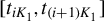 $[t_{iK_1}, t_{(i+1)K_1}]$
that causes the largeness of these two test statistics, since there is likely to be only one detectable jump on
 $(t_{(i-1)K_1}, t_{(i+2)K_1}]$
(as Corollary 5(a) still holds when
 $K_1$
is replaced with
 $2K_1$
). Then we can see that under certain regularity conditions, an
 $\eta _i$
which is larger than
 $\mathcal T_n$
signals the presence of a distinctively large jump on
 $(t_{(i-1)K_1}, t_{(i+1)K_1}],$
and the jump size can be estimated with the robust LAR, as indicated in Corollary 7 below.
The asymptotic distribution shown in (4.4) is derived on the basis that with high probability, most elements in
 $\mathcal S$
belong to
 $\tilde {\mathcal S}(\bar {c}_1).$
Then we require
 $\bar {c}_1$
to be smaller than
 $(1-c_1)/\tilde {\gamma }$
in using the threshold
 $n^{-\bar {c}_1}$
for jump sizes, since roughly speaking, Equation (4.3) implies that most windows only contain jumps whose absolute sizes are at most at the order of
 $n^{(c_1-1)/\tilde {\gamma }}.$
On the other hand,
 $\bar {c}_1$
needs to be larger than
 $\tilde {c}_2/(1-\tilde {\gamma }/2),$
so that given Lemma 2 and Corollary 5(c), the term which absorbs the impact of jumps on
 $\bar {\phi }_i$
for
 $i\in \tilde {\mathcal S}(\bar {c}_1)$
is probably at an order smaller than
 $n^{-\tilde {c}_2}$
(i.e., the order of
 $\bar {g}(n)$
). Also, letting
 $\tilde {c}_2$
be smaller than
 $(2-\tilde {\gamma })(1-c_1)/(2\tilde {\gamma }),$
as required by Corollary 6(b), ensures that
 $\tilde {c}_2/(1-\tilde {\gamma }/2)<(1-c_1)/\tilde {\gamma }.$
As mentioned before, when observing
 $\eta _i>\mathcal T_n$
, we can reasonably expect that there is a relatively large jump on
 $(t_{(i-1)K_1}, t_{(i+1)K_1}],$
and the size of this jump can be estimated with the robust LAR
 $\tilde {\phi }_i$
constructed with data on
 $[t_{((i+1)K_1-K_2)\vee 0}, t_{((i-1)K_1+K_2)\wedge n}].$
Different from our practice in Section 3.3, here we employ the robust instead of the ordinary LAR to estimate the jump sizes. This is because the number of detected jumps may tend to infinity as
 $n\rightarrow \infty $
in the presence of IA jumps, and the robust estimation technique provides the convenience to bound the extreme estimation error in probability. Specifically,
 $\tilde {\phi }_i$
is given by
 $$ \begin{align*}\tilde{\phi}_i=\text{ arg }\ \underset{\phi}{\min}\sum_{j=0}^{K_2-2K_1}\ell_{\beta_0}\left(y_{((i+1)K_1+j)\wedge n}-y_{((i+1)K_1+j-K_2)\vee 0}-\phi\right),\end{align*} $$
and, from now on,
 $K_2$
is assumed to be at the same order as
 $K_1$
in order to simplify the technical analysis, as the impact of jumps on
 $\tilde {\phi }_i$
hinges on the length of the interval
 $[t_{(i+1)K_1-K_2}, t_{(i-1)K_1+K_2}].$
That is, we let
 $K_2= \bar {c}_2K_1$
with some constant integer
 $\bar {c}_2>2.$
Now, we use Corollary 7 to indicate that for each jump whose absolute size is, roughly speaking, at an order larger than
 $n^{(c_1-1)/(2\tilde {\gamma })},$
the difference between its size and the robust LAR is small in probability.
Corollary 7. Under the alternative hypothesis
 $H_1$
and Assumptions 1–4 and 7, for any constants
 $\bar {c}_3\in \left (0, (1-c_1)/(2\tilde {\gamma })\right )$
and
 $\epsilon>0,$
we have
 $$ \begin{align*}\mathrm{P}\left(\bar{N}_{T-,n^{-\bar{c}_3}}>0\right)\overset{n\rightarrow\infty}{\longrightarrow}1,\end{align*} $$
and conditional on
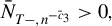 $\bar {N}_{T-,n^{-\bar {c}_3}}>0,$
 $$ \begin{align*}\underset{i\in\bar{\mathcal S}\left(n^{-\bar{c}_3}\right)}{\max} \ \left|\tilde{\phi}_i-\sum_{i=1}^{\bar{N}_{T-,n^{-\bar{c}_3}}}\Delta J_{\bar{\tau}_{i, n^{-\bar{c}_3}}}\boldsymbol 1_{\left\{t_{(i-1)K_1}< \bar{\tau}_{i, n^{-\bar{c}_3}}\leq t_{(i+1)K_1}\right\}}\right|=O_{\mathrm{P}}\left(n^{-\breve{c}_0+\epsilon}\right),\end{align*} $$
where
 $\bar {\mathcal S}(a) :=\left \{i: i\in \mathcal S, \ \text { and } \ \bar {N}_{t_{(i+1)K_1}, a}-\bar {N}_{t_{(i-1)K_1}, a}>0\right \}$
for
 $a>0,$
and
 $\breve {c}_0=\min (\tilde {c}_0, 1-c_1-\bar {c}_3\tilde {\gamma }, (1-c_1)/2+(1-\tilde {\gamma })\bar {c}_3).$
As Corollary 5(a) suggests that there is likely to be at most one jump on
 $(t_{(i-1)K_1}, t_{(i+1)K_1}]$
whose absolute size is larger than
 $n^{-\bar {c}_3}$
for each
 $i\in \mathcal S,$
Corollary 7 indicates that the difference between
 $\tilde {\phi }_i$
and the largest absolute jump size on
 $(t_{(i-1)K_1}, t_{(i+1)K_1}]$
is approximately at the order of
 $n^{-\breve {c}_0}.$
The appearance of terms
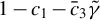 $1-c_1-\bar {c}_3\tilde {\gamma }$
and
 $(1-c_1)/2+(1-\tilde {\gamma })\bar {c}_3$
in the definition of
 $\breve {c}_0$
is due to the effects of small jumps. It is obvious that
 $\breve {c}_0>0$
as
 $\bar {c}_3<(1-c_1)/(2\tilde {\gamma }),$
and a smaller
 $\tilde {\gamma }$
may yield a larger
 $\breve {c}_0,$
which intuitively suggests that errors of estimating the relatively large sizes of jumps tend to become smaller when the small jumps are less vibrant.
4.2 Asymptotic Results for Large T
In this section, we reveal the theoretical properties of the proposed test under the condition where T goes to infinity jointly with
 $n.$
In the case of a fixed T and FA jumps, we can treat both the number of jumps and jump sizes roughly as constants, which provides the convenience for us to prove the theories in Section 3. However, when T goes to infinity as n increases, the number of jumps on
 $(0, T)$
may grow as well, and consequently, the smallest and largest sizes of jumps on
 $(0, T)$
may, respectively, tend to zero and infinity, even when the process
 $J_t$
is assumed to have only FA of jumps. Then an interesting extension is to derive asymptotic theories for the proposed test under the condition where T diverges jointly with
 $n.$
In this case, we consider the null and alternative hypotheses as
 $$ \begin{align*}\tilde{H}_0: \Delta J_t=0 \ \text{ for all } \ t\in(0, \infty), \ \ \text{ and } \ \ \tilde{H}_1: \Delta J_{\tau}\neq 0 \ \text{ for some } \ \tau\in(0, \infty),\end{align*} $$
since different from hypotheses
 $H_0$
and
 $H_1$
,
 $\tilde {H}_0$
and
 $\tilde {H}_1$
do not depend on some specific value of
 $T.$
Given the growth rate of the sample size
 $n, T$
cannot tend to infinity at an arbitrarily fast rate, and we employ Assumption 8 below to bound the magnitude of T relative to
 $n.$
Furthermore, we impose some regularity condition on the jump counting process
 $N_t$
with Assumption 9 as follows.
Assumption 8.
 $T=O\left (n^{c_4}\right )$
for some constant
 $c_4\in \left (0, (1-c_1)/3\right ).$
Assumption 9.
 $J_t$
is an FA pure jump process, and the process
 $N_t$
as given in (2.2) has independent increments. Moreover, there exists some constant c such that
 $$ \begin{align*} \mathrm{P}(N_{T_2}-N_{T_1}>0)<c(T_2-T_1) \end{align*} $$
for all
 $0\leq T_1<T_2<\infty .$
In the high-frequency econometrics literature where both n and T go to infinity, it is typical to assume that the observational times are equally spaced and derive asymptotics under assumptions involving
 $\Delta _n :=t_i-t_{i-1}$
and T jointly (e.g., Kanaya and Kristensen, Reference Kanaya and Kristensen2016; Kanaya, Reference Kanaya2017; Park and Wang, Reference Park and Wang2021; Andersen et al., Reference Andersen, Fusari, Todorov and Varneskov2019). In this article, a relation between
 $\bar {\Delta }_n :=\underset {i}{\max } \ (t_i-t_{i-1})$
and T is introduced by Assumptions 3 and 8, which suggest that
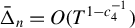 $\bar {\Delta }_n=O(T^{1-c_4^{-1}})$
. Assumption 9 is satisfied when
 $N_t$
follows, for example, the Poisson process, and it implies that uniformly for each
 $i\in \mathcal S,$
there is at most one jump on interval
 $[t_{(i-1)K_1}, t_{(i+1)K_1}]$
with probability approaching one (see Lemma S3 in the Supplementary Material). Then it is unlikely that some jump is not detected due to the disturbance from another jump near it.
When
 $T\rightarrow \infty ,$
Assumption 1 is not enough for us to bound
 $a_t$
and
 $\sigma _t$
(in probability) uniformly over the whole time span. Then we consider Assumption 10 to restrict the magnitudes of
 $ \underset {t\in [0, T]}{\sup }\left |a_t\right |$
and
 $\underset {t\in [0, T]}{\sup }\left |\sigma _t\right |.$
Assumption 10.
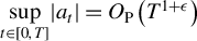 $\underset {t\in [0, T]}{\sup } |a_t|=O_{\mathrm {P}}\left (T^{1+\epsilon }\right )$
and
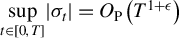 $\underset {t\in [0, T]}{\sup } |\sigma _t|=O_{\mathrm {P}}\left (T^{1+\epsilon }\right )$
for any fixed
 $\epsilon>0$
as
 $T\rightarrow \infty .$
The orders of
 $\underset {t}{\sup } \ |a_t|$
and
 $\underset {t}{\sup } \ |\sigma _t|$
for
 $t\in [0, T]$
can be derived with some regularity conditions concerning the degree of continuity of the processes
 $a_t$
and
 $\sigma _t.$
In particular, the validity of the condition about
 $\sigma _t$
in Assumption 10 can be justified under Assumption S1 which has been employed by Kanaya and Kristensen (Reference Kanaya and Kristensen2016) for the estimation of spot volatilities in the case where
 $T\rightarrow \infty .$
Assumption S1. There exist positive constants
 $c, q_1$
, and
 $q_2$
such that for all
 $s,t\in [0, \infty ),$
 $$ \begin{align*}\mathbb{E}\left(\left|\sigma_t^2-\sigma_s^2\right|{}^{q_1}\right)\leq c\left|t-s\right|{}^{1+q_2}.\end{align*} $$
Assumption S1 imposes a smoothness condition on the volatility process. As pointed out by Kanaya and Kristensen (Reference Kanaya and Kristensen2016), this assumption is satisfied when
 $\left \{\sigma _t\right \}$
follows a drift–diffusion process with the drift and diffusion coefficients subject to certain moment conditions; in particular, Assumption S1 holds when
 $\left \{\sigma _t\right \}$
is an Ornstein–Uhlenbeck or CIR process. Moreover, Lemma A.1 derived by Kanaya and Kristensen (Reference Kanaya and Kristensen2016) suggests that under Assumption S1, the process
 $\sigma _t^2$
is almost surely locally Hölder continuous with exponent d that can take any value on
 $(0, q_2/q_1).$
Then it is natural to see that when
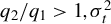 $q_2/q_1>1, \sigma _t^2$
is almost surely time-invariant over the infinite interval
 $[0, \infty ),$
as illustrated in Lemma 3. Moreover, in Lemma 3, we bound the growth rate of
 $\underset {t\in [0, T]}{\sup } |\sigma _t^2|$
almost surely as
 $T\rightarrow \infty $
when
 $q_2/q_1\leq 1.$
Lemma 3. Under Assumption S1, it holds that: (a) if
 $q_2/q_1>1,$
 $$ \begin{align*} \mathrm{P}\left(\underset{t\in[0, \infty)}{\sup} \ \left|\sigma_t^2-\sigma_0^2\right|=0\right)=1; \end{align*} $$
(b) if
 $q_2/q_1\leq 1,$
almost surely
 $$ \begin{align*} \underset{t\in[0, T]}{\sup} |\sigma_t|<T\ln(T)^{1-q_2/q_1+\epsilon} \end{align*} $$
for any fixed
 $\epsilon>0,$
as
 $T\rightarrow \infty .$
Lemma 3 suggests that
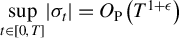 $\underset {t\in [0, T]}{\sup } |\sigma _t|=O_{\mathrm {P}}\left (T^{1+\epsilon }\right )$
for any fixed
 $\epsilon>0$
under Assumption S1. Then Assumption 10 is satisfied under Assumption S1 and the regularity condition for
 $a_t$
assumed in similar fashion as Assumption S1, that is,
 $$ \begin{align*}\mathbb{E}\left(\left|a_t^2-a_s^2\right|{}^{q_1}\right)\leq c\left|t-s\right|{}^{1+q_2}\end{align*} $$
for all
 $s, t\in [0, \infty ).$
Now, we show in Lemma 4 that in the context of growing
 $T, \bar {\phi }_i$
can be still regarded as a valid approximation of the LAR of the efficient price, when the interval
 $(t_{(i-1)K_1}, t_{(i+1)K_1}]$
does not contain a jump whose absolute size is larger than some threshold increasing in
 $n.$
Lemma 4. Under Assumptions 3, 4, and 8–10, for any fixed
 $\epsilon \in (0, \min (\bar {c}_0/2, (c_1-\bar {c}_0)/2)),$
we have
 $$ \begin{align*}\underset{i\in\tilde{\mathcal S}\left(n^{\bar{c}_0/2-\epsilon}\right)}{\max} \left|\bar{\phi}_i -\sum_{j=0}^{K_1}(x_{iK_1+j}-x_{(i-1)K_1+j})/(K_1+1)\right|=O_{\mathrm{P}}\left(n^{-2\epsilon}\right)\end{align*} $$
as
 $n, T\rightarrow \infty .$
Comparing Lemmas 1 and 4, we can see that in the absence of jumps, the difference between
 $\bar {\phi }_i$
and
 $\sum _{j=0}^{K_1}(x_{iK_1+j}-x_{(i-1)K_1+j})/(K_1+1)$
is approximately at the order of
 $n^{\max (-\bar {c}_0, \bar {c}_0-c_1)},$
no matter whether T goes to infinity or not. However, when
 $T\rightarrow \infty ,$
we can reveal the order of the difference between
 $\bar {\phi }_i$
and
 $\sum _{j=0}^{K_1}(x_{iK_1+j}-x_{(i-1)K_1+j})/(K_1+1)$
only for the condition where the order of the possible jump size that affects
 $\bar {\phi }_i$
is smaller than
 $n^{\bar {c}_0/2},$
as shown in Lemma 4. Nevertheless, a jump whose absolute size is not smaller than
 $n^{\bar {c}_0/2}$
is still likely to substantially enlarge some robust LAR, according to Corollary 8, which describes the behaviors of
 $\bar {\phi }_i$
in the context of growing
 $T.$
Corollary 8.
(a) For any fixed
 $\breve {\epsilon }_0>0$
and
 $\epsilon>0,$
under Assumptions 3, 4, and 8–10, we have
 $$ \begin{align} \underset{i\in\tilde{\mathcal S}\left(n^{-\tilde{c}_2-\breve{\epsilon}_0}\right)}{\max} \left|\bar{\phi}_i\right|=O_{\mathrm{P}}\left(n^{-\tilde{c}_3+\epsilon}\right) \end{align} $$
for
 $\tilde {c}_3=\min \left (\bar {c}_0, c_1-\bar {c}_0, \tilde {c}_2+\breve {\epsilon }_0, (1-c_1-3c_4)/2\right ),$
as
 $n, T\rightarrow \infty .$
(b) Recall the definitions of
 $\bar {N}_{t,x}, \bar {h}_{i,x}$
, and
 $\bar {\tau }_{i,x}$
given in Corollary 5. Under the alternative hypothesis
 $\tilde {H}_1$
and Assumptions 3, 4, and 8–10, for any constants
 $\bar {\epsilon }_0>0, \bar {\epsilon }_1\in (0, \tilde {c}_3) $
and
 $\tilde {c}_1<1/2,$
we have
 $$ \begin{align} \mathrm{P}\left(\bar{N}_{T-,n^{-\tilde{c}_3+\bar{\epsilon}_1}}>0, \ \text{ and } \ \underset{i\in\{1,\ldots , \bar{N}_{T-,n^{-\tilde{c}_3+\bar{\epsilon}_1}}\}}{\min}\bar{f}_i=1 \right)\overset{n, T\rightarrow\infty}{\longrightarrow}1 \end{align} $$
with
 $\bar {f}_i :=\boldsymbol 1_{\left \{\bar {h}_{i,n^{-\tilde {c}_3+\bar {\epsilon }_1}}\in \mathcal S, \ \text { and } \ |\bar {\phi }_{\bar {h}_{i,n^{-\tilde {c}_3+\bar {\epsilon }_1}}}|>\tilde {c}_1\left (|\Delta J_{\bar {\tau }_{i, n^{-\tilde {c}_3+\bar {\epsilon }_1}}}|\wedge n^{\bar {c}_0/2-\bar {\epsilon }_0}\right )\right \}}$
.
Corollary 8(a) uniformly bounds the magnitudes of the
 $\bar {\phi }_i$
’s which are unaffected by jumps or affected by jumps whose sizes are at a smaller order than
 $\bar {g}_n$
in probability. The convergence in (4.6) indicates that for a jump on
 $(0, T)$
with a non-negligible size, it is likely to significantly increase the magnitude of at least one
 $\bar {\phi }_i.$
We have to add the threshold
 $n^{\bar {c}_0/2-\bar {\epsilon }_0}$
in the definition of
 $\bar {f}_i,$
given the difficulty in bounding the difference between
 $\bar {\phi }_i$
and the corresponding LAR due to overly large jumps. Then a limitation of Corollary 8 is that it fails to provide an explicit relation between the size of a jump which is at an order not smaller than
 $n^{\bar {c}_0/2}$
and the corresponding robust LAR. However, from (4.6), it can be seen that such jumps are likely to cause the corresponding
 $|\bar {\phi }_i|$
’s to be large.
Given the results in Corollary 8, we illustrate the properties of
 $\eta _i$
’s to justify the sizes and powers of our test in Corollary 9. Analogous to Theorem 1 and Corollary 6(b), Corollary 9 reveals the asymptotic behavior of the maximum of the
 $\eta _i$
’s associated with the windows that do not contain jumps or contain only small jumps. Moreover, Corollary 9 roughly suggests that the jumps whose sizes are at an order larger than
 $n^{-\tilde {c}_2}$
are likely to be detected by the proposed test.
Corollary 9. Suppose that
 $\tilde {c}_2<(1-c_1-3c_4)/2$
and Assumptions 3, 4, and 8–10 hold. For any fixed
 $\bar {x}\in \mathbb {R}$
and
 $\epsilon>0,$
we have
 $$ \begin{align} \mathrm{P}\left(\underset{i\in\tilde{\mathcal S}\left(n^{-\tilde{c}_2-\epsilon}\right)}{\max} \left(\eta_i-\bar{a}_n\right)/\bar{b}_n\leq\bar{x}\right)\overset{n\rightarrow\infty}{\longrightarrow} \exp\left(-e^{-\bar{x}}\right), \end{align} $$
and under the alternative hypothesis
 $\tilde {H}_1,$
 $$ \begin{align} \mathrm{P}\left(\bar{N}_{T-,n^{-\tilde{c}_2+\bar{\epsilon}_2}}>0, \ \text{ and } \ \underset{i\in\{1,\ldots , \bar{N}_{T-,n^{-\tilde{c}_2+\bar{\epsilon}_2}}\}}{\cap}\bar{\mathcal{A}}_i \right)\overset{n, T\rightarrow\infty}{\longrightarrow}1 \end{align} $$
for any fixed
 $\bar {\epsilon }_2\in (0, \tilde {c}_2),$
where
 $\bar {\mathcal A}_i:=\{\bar {h}_{i,n^{-\tilde {c}_2+\bar {\epsilon }_2}}\in \mathcal S, \ \text { and } \ \eta _{\bar {h}_{i,n^{-\tilde {c}_2+\bar {\epsilon }_2}}}>\mathcal T_n\}.$
We may not detect all jumps on
 $(0, T)$
as
 $n, T\rightarrow \infty ,$
since there may exist jumps whose absolute sizes are too small to substantially enlarge the corresponding
 $\eta _i$
’s. Accordingly, (4.7) concerns jumps whose sizes are at an order smaller than
 $n^{-\tilde {c}_2}.$
Given the proof of (4.7), it is trivial to verify that this convergence still holds when the set
 $\tilde {\mathcal S}\left (n^{-\tilde {c}_2-\epsilon }\right )$
is replaced with
 $\mathcal S_0.$
Then a comparison between (4.7) and the result in Theorem 1 suggests that under certain regularity conditions, letting
 $T\rightarrow \infty $
does not change the asymptotic behavior of the maximum
 $\eta _i$
for
 $i\in \mathcal S_0.$
On the other hand, (4.8) implies that as
 $n, T\rightarrow \infty ,$
the lower bound of detectable jump sizes in absolute value is allowed to approach zero roughly at the rate of
 $n^{-\tilde {c}_2}.$
Based on steps similar to those in the proof of Lemma S3 in the Supplementary Material, it can be checked that with probability approaching one, for each
 $i\in \mathcal S,$
there is no more than one jump within the interval
 $\left [t_{(i-1)K_1}, t_{((i+2)K_1)\wedge n}\right ]$
as
 $n, T\rightarrow \infty .$
Thus, when both
 $\eta _i$
and
 $\eta _{i+1}$
are larger than
 $\mathcal T_n,$
it is likely to be the same jump within
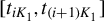 $[t_{iK_1}, t_{(i+1)K_1}]$
that causes the largeness of these two statistics. Accordingly, we can still use
 $\hat {N}$
as the estimator for the number of detected jumps. Since
 $N_T$
may go to infinity when
 $T\rightarrow \infty ,$
we can use the robust version of the LAR
 $\bar {y}_i$
’s, which are
 $\tilde {\phi }_i$
’s given by
 $$ \begin{align*}\tilde{\phi}_i=\text{ arg }\ \underset{\phi}{\min}\sum_{j=0}^{K_2-2K_1}\ell_{\beta_0}\left(y_{((i+1)K_1+j)\wedge n}-y_{((i+1)K_1+j-K_2)\vee 0}-\phi\right),\end{align*} $$
to estimate the sizes of detected jumps. It can be readily shown that the difference between
 $\tilde {\phi }_i$
and the jump size on
 $(t_{(i-1)K_1}, t_{(i+1)K_1}]$
is small in probability uniformly across
 $i\in \mathcal S_2,$
as illustrated in Corollary 10 below.
Corollary 10. Under the alternative hypothesis
 $\tilde {H}_1$
and Assumptions 3, 4, and 8–10, we have
 $$ \begin{align*} \underset{i\in\mathcal S_2}{\max} \ \left|\tilde{\phi}_i-\sum_{\ell=1}^{N_{T-}}\Delta J_{\tau_\ell}\boldsymbol 1_{\left\{\tau_\ell\in (t_{(i-1)K_1}, t_{(i+1)K_1}]\right\}}\right|=O_{\mathrm{P}}\left(n^{-\tilde{c}_3+\epsilon}\right) \end{align*} $$
for any fixed
 $\epsilon>0.$
Corollary 10 is proved based on the union of two principles: First, in the absence of jumps,
 $\tilde {\phi }_i$
’s would be approximately at the order of
 $n^{-\tilde {c}_3}$
uniformly across
 $i\in \mathcal S.$
Second, with high probability, the effect of a jump on
 $[t_{(i-1)K_1}, t_{(i+1)K_1}]$
is to increase or decrease (depending on the sign of this jump)
 $\tilde {\phi }_i$
by the absolute jump size.
5 SIMULATIONS
In this section, we perform simulation studies to examine the finite sample performance of our test and compare it with the tests proposed by Lee and Mykland (Reference Lee and Mykland2012) and Sun (Reference Sun2019). We simulate the dynamics of the efficient price based on Equation (2.1), and let the drift coefficient
 $a_t=0.$
We consider three data generating processes (DGPs) introduced below to simulate the volatility
 $\sigma _t$
and noises
 $u_i.$
DGP 1. Time-Varying Volatility and MA(1) Noises. Following Andersen and Bollerslev (Reference Andersen and Bollerslev1998) and Laurent and Shi (Reference Laurent and Shi2020), we adopt the model below to generate the process
 $\sigma _t$
:
 $$ \begin{align} d\sigma_t^2=\kappa\left(\bar{\sigma}-\sigma_t^2\right)dt+\sqrt{2\lambda\kappa}\sigma_t^2dW_t, \ \ t\in(0, T], \end{align} $$
where
 $\lambda =0.296,$
the long-run mean of the process
 $\bar {\sigma }=10^{-4},$
the starting value
 $\sigma _0^2$
also equals
 $10^{-4},$
the mean-reversion parameter
 $\kappa =0.035,$
and
 $W_t$
is an independent standard Brownian motion. Under Equation (5.1), the diffusion process
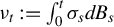 $\nu _t :=\int _0^t\sigma _sdB_s$
is driven by the continuous-time limit version of the GARCH model (see Drost and Werker, Reference Drost and Werker1996), and Assumption S1 is satisfied, as pointed out by Kanaya and Kristensen (Reference Kanaya and Kristensen2016, Sect. 8). We let the noises follow the first-order moving average (MA(1)) process. That is,
 $$ \begin{align*} u_i=\left(1+\theta_u^2\right)^{-1/2}\left(\tilde{\eta}_i+\theta_u\tilde{\eta}_{i-1}\right), \end{align*} $$
where
 $\tilde {\eta }_i\overset {i.i.d.}{\sim }\mathcal N (0, \bar \omega ), \bar \omega =\bar {\varphi }_0\bar {\sigma }$
with the noise-to-signal ratio
 $\bar {\varphi }_0\in \{0.001, 0.002, 0.005\}$
and
 $\theta _u=0.5,$
which is in line with the simulation designs of Barndorff-Nielsen et al. (Reference Barndorff-Nielsen, Hansen, Lunde and Shephard2011, Sect. 6.1.2) and Varneskov (Reference Varneskov2017).
DGP 2. Time-Varying Volatility and Heteroskedastic Noises with Fatter Tails in Distribution. We still employ Equation (5.1) and choose the same parameter values to generate
 $\sigma _t.$
For each
 $i,$
the noise
 $u_i$
is independently generated as
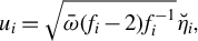 $u_i=\sqrt {\bar \omega (f_i-2)f_i^{-1}}\breve {\eta }_i,$
where conditional on
 $f_i, \breve {\eta }_i$
is subject to the student’s t-distribution with degree of freedom being
 $f_i,$
and
 $f_i$
is given by
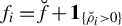 $f_i=\breve {f}+\boldsymbol 1_{\left \{\breve {\rho }_i>0\right \}}$
with
 $\breve {f}=5$
and
 $\breve {\rho }_i$
independently drawn from the Bernoulli distribution given by
 $\mathrm {P}\left (\breve {\rho }_i=0\right )=\mathrm {P}\left (\breve {\rho }_i=1\right )=1/2.$
Here, we incorporate the component
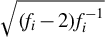 $\sqrt {(f_i-2)f_i^{-1}}$
into the rescaling coefficient as
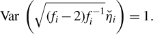 $\text { Var }\left (\sqrt {(f_i-2)f_i^{-1}}\breve {\eta }_i\right )=1.$
DGP 3. Constant Volatility and Independent Gaussian Noises. We set
 $\sigma _t=10^{-2}$
for all
 $t\in [0, T],$
and
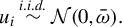 $u_i\overset {i.i.d.}{\sim } \mathcal N (0, \bar \omega ).$
In all DGPs, we let
 $T=1$
represent 1 trading day with 6.5 working hours, so that 1 second is normalized to
 $1/(3,600\times 6.5).$
We generate
 $\lfloor T\rfloor $
jumps in each replication. Unless stated otherwise, we independently draw jump arrival times and jump sizes from the uniform distribution on
 $[0, T]$
and the Gaussian distribution
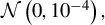 $\mathcal N\left (0, 10^{-4}\right ),$
respectively, as we consider different values for T in numerical studies. In generating the artificial randomness, we set the distribution
 $\mathcal D$
as
 $\mathcal N(0, 1).$
The observational times are equally spaced, and we consider three sampling frequencies, including
 $\Delta _n :=t_i-t_{i-1}\in \{4, 6, 10\}$
seconds. Moreover, the significance level
 $\alpha =0.05,$
and all the results reported in this section are based on 1,000 replications.
There are four tuning parameters (i.e.,
 $K_1, \beta _0, L_n$
, and
 $\bar {g}_n$
) involved in the proposed test, and they are defined in the form as
 $cn^b$
or
 $cn^{-b}$
for positive constants b and c; we first specify orders of the parameters (i.e., b’s) given the regularity conditions and theoretical results, and then choose the coefficients (i.e., c’s). In particular, we choose
 $\bar {c}_0=1/4$
and
 $c_1=1/2,$
since Corollary 1(a) suggests that such a choice can minimize the order of
 $\bar {\phi }_i$
’s unaffected by jumps. Moreover, any choice for
 $\tilde {c}_2$
and
 $c_2$
that satisfy
 $\tilde {c}_2\in (0, \tilde {c}_0)$
and
 $c_2>2(1-c_1)$
are in line with the regularity conditions stated in Section 3, and then we simply choose
 $\tilde {c}_2=1/8$
and
 $c_2=1.05.$
As the volatility is critical for the magnitudes of efficient price increments over small intervals in the absence of jumps, we find that letting the coefficient of
 $\bar {g}_n$
incorporate some volatility measure can improve the performance of the test, and thus set
 $\bar {g}_n=c\left (\hat {\sigma }/T\right )^{1/2}n^{-1/8}.$
Here,
 $\hat {\sigma }$
is the truncated realized variance estimator proposed by Mancini (Reference Mancini2009) based on 10-minute returns, and
 $\left (\hat {\sigma }/T\right )^{1/2}$
can be regarded as a pilot estimator on the average level of the spot volatility. To sum up, currently, we have defined
 $K_1=\lfloor c_{K}n^{1/2}\rfloor , \beta _0=c_{\beta }n^{1/4}, L_n=\lfloor c_Ln^{1.05}\rfloor ,$
and
 $\bar {g}_n=c_{g}\left (\hat {\sigma }/T\right )^{1/2}n^{-1/8},$
with
 $c_{K}, c_{\beta }, c_L,$
and
 $c_g$
being positive constants whose values are to be determined.
In the preliminary simulation studies, we find that the choice of
 $c_{K_1}=0.2, c_{L}=1,$
and
 $c_g=2.1$
can yield satisfactory performance of the test for
 $T=1,$
while the test efficiency is insensitive to the value of
 $c_\beta .$
In order to justify this finding, we present the results of sensitivity analysis concerning the size and power of the test with respect to different combinations of the tuning parameters for DGP 1 with
 $\bar {\varphi }_0=0.002$
and
 $\Delta _n=6$
seconds in Tables 1 and 2. Here, the empirical size and power, respectively, mean the empirical probability of the GTE and the proportion of jumps detected by the test. We employ the IRLS approach as described by Qin and Fang (Reference Qin and Fang2023) to obtain the robust LAR
 $\bar {\phi }_i.$
Although we only demonstrate the uniqueness of
 $\bar {\phi }_i$
for the condition where
 $K_1$
is even (cf. Lemma S1 in the Supplementary Material), we do not adjust the value of
 $K_1$
to make it even in numerical studies, since whether it is even or odd does not have an obvious impact on the test efficiency. We also consider the choice of
 $c_\beta =\infty $
(which makes
 $\bar {\phi }_i=\phi _i$
) in Tables 1 and 2, since given price observations, the robust LAR
 $\bar {\phi }_i$
would equal the ordinary LAR
 $\phi _i$
defined in Section 3.1 for all i when
 $c_{\beta }$
is sufficiently large.
Empirical sizes of the proposed test with respect to different tuning parameters

Note: For each main entry, the corresponding values of
 $(c_K, c_g, c_\beta , c_L)$
are either specified at the headings of rows and columns, or (if unspecified at the headings) fixed at the benchmark choices given by
 $(c_K, c_g, c_\beta , c_L)=(0.2, 2.1, 0.01, 1).$
The displayed results are obtained under DGP 1,
 $T=1, \Delta _n=6$
seconds, and
 $\bar {\varphi }_0=0.002.$
Empirical powers of the proposed test with respect to different tuning parameters

Note: For each main entry, the corresponding values of
 $(c_K, c_g, c_\beta , c_L)$
are either specified at the headings of rows and columns, or (if unspecified at the headings) fixed at the benchmark choices given by
 $(c_K, c_g, c_\beta , c_L)=(0.2, 2.1, 0.01, 1).$
The displayed results are obtained under DGP 1,
 $T=1, \Delta _n=6$
seconds, and
 $\bar {\varphi }_0=0.002.$
The results suggest that when
 $c_K\in (0.15, 0.25)$
and all the other parameter values are fixed at the benchmark choices, the test efficiency is in general satisfactory and insensitive to the value of
 $c_K.$
However, there seems to be an upward size distortion when
 $c_K$
increases to 0.3, and the test power tends to decline when
 $c_K$
decreases to 0.1. One possible reason for the upward size distortion may be that a larger
 $c_{K}$
can increase the overall magnitude of
 $|\bar {\phi }_i|$
’s unaffected by jumps by enlarging the impact of the continuous component in the price. On the other hand, when
 $c_K$
is relatively small, the noise may have larger effects on the test and thus disturb the detection of jumps. It can be seen that a relatively small
 $c_g$
leads to an upward size distortion. This is natural, since
 $\bar {g}_n$
is supposed to be substantially larger than
 $\underset {i\in \mathcal S_0}{\max } \ \left |\bar {\phi }_i\right |$
in order to make the empirical size close to the significance level. On the other hand, increasing
 $c_g$
can decrease the power, as a larger
 $c_g$
can decrease the value of
 $\eta _i.$
Moreover, the results are basically insensitive to the value of
 $c_L$
when it is not smaller than one, while a small
 $c_L$
(i.e.,
 $c_L=0.5$
) can induce a downward power distortion, which is reasonable as Corollary 2 suggests that a large
 $L_n$
serves to enlarge the impact of jumps on the randomized statistics. To sum up, the test efficiency is not overly sensitive to the parameter values when they vary within reasonable ranges, and the choice of
 $(c_K, c_g, c_L)=(0.2, 2.1, 1)$
delivers good performance of the test in terms of both the power and size. In addition, the test efficiency is insensitive to the choice of
 $c_\beta ,$
since with all the other coefficients unchanged, the variation of
 $c_\beta $
does not incur substantial difference in the results. It seems difficult to theoretically analyze the behavior of
 $\bar {\phi }_i$
when
 $\beta _0$
is small, while in the context of Gaussian noises, it is not surprising to see that the test performs well when we simply employ the ordinary LAR
 $\phi _i$
instead of
 $\bar {\phi }_i$
to construct the test. In particular, under DGP 1, it is straightforward to verify that Equation (3.2) still holds when we replace
 $\bar {\phi }_i$
and
 $\bar {c}_0$
therein, respectively, with
 $\phi _i$
and
 $c_1/2,$
since
 $$ \begin{align*}\phi_i-\sum_{j=0}^{K_1}(x_{iK_1+j}-x_{(i-1)K_1+j})/(K_1+1)=\sum_{j=0}^{K_1}(u_{iK_1+j}-u_{(i-1)K_1+j})/(K_1+1),\end{align*} $$
and the magnitude of the maximum of the noise averages can be easily bounded in probability with the extreme value theory developed by Galambos (Reference Galambos1978) for Gaussian variables. Then, under
 $(c_K, c_g, c_L)=(0.2, 2.1, 1), T=1,$
and
 $\bar {\varphi }_0=0.002,$
we further examine the sensitivity of the test to
 $c_\beta $
with different sampling frequencies in DGP 2, where the noise terms are heteroskedastic and have fatter tails in distribution than Gaussian variables. The corresponding results are shown in Table 3. We can see that the test efficiency is still insensitive to the value of
 $c_\beta ,$
and in particular, the test performs well when
 $c_\beta =\infty .$
Furthermore, the unreported simulation results suggest that the choice of
 $c_{\beta }$
does not substantially affect the performance of the test as values of T and/or
 $\bar {\varphi }_0$
vary. Then we replace
 $\bar {\phi }_i$
with
 $\phi _i$
in constructing the proposed test for the remaining numerical studies (including simulations in the Supplementary Material), although the use of
 $\bar {\phi }_i$
can provide convenience for us to bound the impact of noises in probability under mild regularity conditions.
Sensitivity of the test efficiency to
 $c_\beta $

Note: The main entries report empirical sizes (the numbers on the left) and powers of the proposed test under DGP 2,
 $T=1$
and
 $\bar {\varphi }_0=0.002$
.
We examine the performance of the proposed test with
 $(c_K, c_g, c_L)=(0.2, 2.1, 1)$
for
 $T>1,$
and the unreported simulation results indicate that the increase of T can cause a non-negligible upward size distortion. Then we propose to let orders of the parameters
 $(K_1, L_n, \bar {g}_n)$
be determined by the average number of observations within one day, while the constant coefficients remain unchanged; that is,
 $$ \begin{align} K_1=\lfloor 0.2\left(n/T\right)^{1/2}\rfloor, \ L_n=\lfloor (n/T)^{1.1}\rfloor \ \ \text{ and } \ \ \bar{g}_n=2.1\left(\widehat{\sigma}/T\right)^{1/2}(n/T)^{-1/8}. \end{align} $$
The specification in (5.2) can largely smooth away the impact of T on parameters
 $K_1, L_n,$
and
 $\bar {g}_n.$
Then we can reasonably expect that when the sampling frequency is sufficiently high and T becomes moderately larger, the approximate normality of the randomized statistics unaffected by jumps is not substantially affected by the increase of
 $T,$
and the empirical size of the test could stay close to the significance level. We show the performance of the test constructed with the parameters given by (5.2) under different values of T and
 $\bar {\varphi }_0=0.002$
for the three DGPs in Table 4. It seems that the test generally performs well across the various scenarios, and in particular, the size is basically robust to the growth of
 $T.$
Moreover, the moderate downward distortion of the power due to the increase of T can be relieved by the use of more frequent observations. Then, in the remaining numerical studies, we stick to the tuning parameters as shown in (5.2).
Performance of our test

Note: The main entries report empirical sizes (the numbers on the left) and powers of the proposed test under
 $\bar {\varphi }_0=0.002$
.
We compare the finite sample performance of our test with the jump tests developed by Lee and Mykland (Reference Lee and Mykland2012) and Sun (Reference Sun2019). For the three DGPs under consideration, only DGP 3 is in line with the regularity conditions assumed by Lee and Mykland (Reference Lee and Mykland2012) and Sun (Reference Sun2019), since LM12 (Lee and Mykland, Reference Lee and Mykland2012) requires the spot volatility to be constant over time, and Sun (Reference Sun2019) does not allow noises to be serially-dependent or drawn from the student’s t-distribution. Moreover, LM12 assumes the noise terms as stationary in distribution, which is not in line with the heteroskedasticity property of noises in DGP 2. In this set of experiments, we choose
 $T=1$
and follow the instructions given by LM12 and Sun (Reference Sun2019) to construct their tests. We report the empirical sizes and powers of the tests in Table 5. It can be seen that the empirical sizes of all the tests are satisfactory, and our test has a moderate advantage over the other two in terms of the power. The performance of the LM12 test is basically acceptable across the scenarios, and it has higher powers than the test by Sun (Reference Sun2019). The time variation in the volatility and the heteroskedasticity in the noise seem not to substantially affect the performance of the LM12 test, in spite of the theoretical limitation of this test. Moreover, the power of Sun’s (Reference Sun2019) test is lower in DGP 1 than in DGPs 2 and 3, which suggests that its power is numerically vulnerable to serial dependence in the noise. For all the three tests, the powers increase as we employ more frequent observations.
Empirical sizes and powers of the three tests

Note: LM, Sun1, and Sun2 represent the tests proposed by Lee and Mykland (Reference Lee and Mykland2012), Sun (Reference Sun2019), and this article, respectively. The main entries report the empirical sizes (the numbers on the left) and powers of the corresponding tests under
 $T=1$
.
To further investigate the power of each test, we let the jump size vary within
 $[0.3\%, 0.6\%],$
and compute the empirical powers of the tests with
 $\bar {\varphi }_0=0.005, T=1,$
and the sampling frequency being 6 seconds. The outcome is displayed in the plots of Figure 3, which indicates the steady growth of the powers as the jump size increases. In line with the results in Table 5, the plots suggest that our test has higher powers than the other two tests, and this advantage seems robust as the jump size varies within the range under consideration. Figure 3 suggests that in the scenarios under consideration, it is difficult for our test to detect jumps whose sizes are not larger than
 $0.3\%,$
since when the jump size equals
 $0.3\%,$
the empirical powers of our test are only 0.25, 0.24, and 0.32 for DGPs 1–3, respectively. With
 $\Delta _n$
decreasing from 6 seconds to 4 seconds and all the other conditions unchanged, we find that the empirical powers of our test for the jump size of
 $0.3\%$
are still quite small, as the powers increase only to 0.29, 0.27, and 0.36 under DGPs 1–3, respectively. Then it is not surprising to see that the powers of our test displayed in Table 5 are not quite close to one, since a non-negligible portion of jumps may not be sufficiently large for our test to detect, given that the distribution we choose to generate the jump size is
 $\mathcal N \left (0, 10^{-4}\right )$
in obtaining the results in Table 5.
Empirical powers of the three tests with respect to different jump sizes under
 $T=1, \bar {\varphi }_0=0.005,$
and
 $\Delta _n=6$
seconds. LM, Sun1, and Sun2 represent the tests proposed by Lee and Mykland (Reference Lee and Mykland2012), Sun (Reference Sun2019), and this article, respectively.

As mentioned before, Lee and Mykland (Reference Lee and Mykland2012) and Sun (Reference Sun2019) require the spot volatility to be constant or continuous, while our test does not rely on such a regularity condition. Then we also study the efficiency of the three tests under the DGPs where there are jumps in the process of the volatility, and present the results concerning the empirical sizes and powers in Table S1 in the Supplementary Material. As specified therein, the corresponding DGPs, which are denoted as DGPs 1.1–1.3, are the same as DGPs 1–3, except that jump components are inserted in the volatility processes under DGPs 1.1–1.3. A comparison of the results in Table 5 and Table S1 in the Supplementary Material suggests that volatility jumps can decrease powers of all the three tests. Although our test is asymptotically immune to discontinuities on the path of the volatility, volatility jumps make the spot volatility in general more volatile, and thus can compromise the effect of the truncated realized variance (i.e.,
 $\hat {\sigma }$
) in improving the finite sample performance of the test, since we employ
 $\left (\hat {\sigma }/T\right )^{1/2}$
as a measure on the overall level of the spot volatility. Also, the results imply that volatility jumps can cause an upward distortion in the size of the LM12 test, while this issue can be relieved with more frequent observations. On the other hand, the sizes of our and Sun’s (Reference Sun2019) tests are basically close to the significance level 0.05 under DGPs 1.1–1.3.
We investigate the finite sample performance of the jump number estimator, that is,
 $\hat {N}$
defined in Section 3.3, and show the results in Table 6. This time we let
 $T=3$
and
 $\bar {\varphi }_0=0.005,$
with sizes of the three jumps independently drawn from the distribution
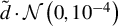 $\tilde {d}\cdot \mathcal N \left (0,10^{-4}\right )$
for
 $\tilde {d}\in \{1, 2, 3\}.$
From Table 6, we can see that underestimation is much more common than overestimation. Consequently, the average estimator would be closer to 3 when d becomes larger, or more frequent observations are employed, which can improve the power of the test.
Results for estimating the number of jumps

Note: In each main entry, the number outside the parentheses is the average of the jump number estimators over the 1,000 trials; the three numbers in the parentheses are, respectively, the percentages of times that the estimator is equal to (in the middle), smaller (on the left), and larger than the number of jumps, that is, 3. The displayed results are obtained under
 $T=3$
and
 $\bar {\varphi }_0=0.005.$
We perform experiments to evaluate the efficiency of the LAR
 $\bar {y}_i$
described in Section 3.3 as a jump size estimator, with the tuning parameter
 $K_2=3K_1.$
We can also estimate jump sizes with the robust LAR
 $\tilde {\phi }_i$
as suggested in Sections 4.1 and 4.2, but the unreported estimation results, respectively, given by
 $\bar {y}_i$
and
 $\tilde {\phi }_i$
are similar. We let
 $T=20$
in this set of simulations. Unless a jump is very close to times zero or
 $T,$
it is contained in intervals
 $[t_{(i-1)K_1}, t_{(i+1)K_1}]$
for two consecutive i’s
 $\in \mathcal S,$
and we select the smaller i in evaluating the estimation accuracy for the jump size. In each of the 1,000 trials, we consider the maximum and medium errors in absolute values across the size estimation for the 20 jumps and report the means of these errors over all the trials in Table 7. From the results, we can see that the estimation errors increase when the noise-to-signal ratio
 $\bar {\varphi }_0$
becomes larger, and decrease when we employ more frequent observations.
The mean errors (‰) of estimating jump sizes

Note: The two numbers in each main entry are the means over the 1,000 trials of, respectively, the maximum and medium absolute errors (‰) of estimating the sizes of 20 jumps in one trial for
 $T=20.$
As mentioned before, in the Supplementary Material, we derive a test to examine whether there are jumps at given time points, and a simulation study is carried out in Section 2.2 therein to evaluate the finite sample performance of this test. It turns out that across all the DGPs under consideration, the empirical probabilities of the GTE grow rapidly as the number of time points considered in the null hypothesis increases, when the test threshold (i.e., the counterpart of
 $\mathcal T_n$
) is chosen only to satisfy the local consistency. In contrast, the empirical probabilities of the GTE are basically close to the significance level when the global consistency is achieved. This illustrates the importance of determining the test threshold according to the global property of the statistics for multiple (or sequential) jump tests.
We also investigate the performance of the proposed test when the jump process has IA in Section 2.3 in the Supplementary Material, and in line with our theories, the corresponding simulation results suggest that: (i) more frequent observations enable us to detect smaller jumps and (ii) most time windows considered in the test do not contain jumps whose absolute sizes are larger than some quantity which tends to zero as n grows, and the maximum of the randomized statistics associated with these windows is unlikely to be larger than the test threshold
 $\mathcal T_n.$
6 REAL DATA EXAMPLES
In this section, we apply the proposed test to the transaction price data collected from the TAQ database for the stocks of Apple and Microsoft and the period from 10 February 2020 to 20 March 2020, which includes 29 trading days. Both stocks were heavily traded, since there are
 $1.64\times 10^7$
and
 $1.55\times 10^7$
tick-by-tick observations, respectively, for Apple and Microsoft during the trading hours (9:30–16:00) of the sampling period. We perform the test with data subsampled from the original observations and adopt the parameter
 $\triangle \zeta \!\in \!\{4, 6, 10\}$
seconds to control the subsampling frequency. Specifically, when
 $t_i,$
that is, the observation time of the ith price in the test sample, is given,
 $t_{i+1}$
is determined by
 $$ \begin{align*}t_{i+1}=\underset{t\in\mathcal B}{\min} \ (t-t_i)\geq\triangle\zeta,\end{align*} $$
where
 $\mathcal B$
is the set containing observation times of all the price data. The parameters for the test and estimation are chosen in the same way as specified in the simulation studies. The arrival times and estimated sizes of the detected jumps, along with the time paths of the stock prices (in logarithmic values), are plotted in Figures 4 and 5. We also show some statistics about the estimated jump sizes in Tables 8 and 9.
We use the solid line to show the time path of the Apple stock price, and circles to mark the arrival times and estimated sizes of the detected jumps. The values of
 $\Delta \zeta $
that we choose in constructing the test are
 $\Delta \zeta =10$
seconds,
 $\Delta \zeta =6$
seconds, and
 $\Delta \zeta =4$
seconds, respectively, for the three plots from the left to the right. The main labels under the ticks in the horizontal axis represent the numbers of hours between the tick times and the beginning time, that is, 9:30 on 10 February 2020.

We use the solid line to show the time path of the Microsoft stock price, and circles to mark the arrival times and estimated sizes of the detected jumps. The values of
 $\Delta \zeta $
that we choose in constructing the test are
 $\Delta \zeta =10$
seconds,
 $\Delta \zeta =6$
seconds, and
 $\Delta \zeta =4$
seconds, respectively, for the three plots from the left to the right. The main labels under the ticks in the horizontal axis represent the numbers of hours between the tick times and the beginning time, that is, 9:30 on 10 February 2020

Statistics of estimated jump sizes for Apple

Note: This table includes the numbers of detected jumps, the means, standard deviations (SD), minimums (Min), and maximums (Max) of the estimated jump sizes, as well as the means of the absolute values of the estimated jump sizes (Abs. Mean).
Statistics of estimated jump sizes for Microsoft

Note: This table includes the numbers of detected jumps, the means, standard deviations (SD), minimums (Min), and maximums (Max) of the estimated jump sizes, as well as the means of the absolute values of the estimated jump sizes (Abs. Mean).
We can see that for each stock, data sampled at different frequencies deliver similar patterns of the arrival times of detected jumps, and more jumps can be detected with the use of more frequent observations. It is natural to see in Tables 8 and 9 that the average sizes (in absolute value) of detected jumps decrease when
 $\triangle \zeta $
shrinks, since more frequent observations may improve the power of the test by enabling us to identify smaller jumps, as implied by Corollary 6(a). The figures show that the jump occurrences were not evenly distributed. Specifically, for both stocks, jump arrivals were relatively rare in the first week of the sampling period, but the jump intensity seems to increase drastically in the second half of the period, when the stock market crash occurred due to the COVID-19 pandemic (Mazur, Dang, and Vega, Reference Mazur, Dang and Vega2021), and drastic changes in the stock prices of Apple and Microsoft were quite often (as can be seen from the time paths of the prices). In particular, for both stocks, the clumps of jumps detected during the second half of the period suggest patterns of self-exciting jump clusters (see, e.g., Fulop et al., Reference Fulop, Li and Yu2015; Maneesoonthorn, Forbes, and Martin, Reference Maneesoonthorn, Forbes and Martin2017; Bowwijk, Laeven, and Yang, Reference Bowwijk, Laeven and Yang2018), and it seems that such jump clustering patterns are more obvious when more frequent observations are employed to build the test. This phenomenon is unsurprising, since for two jumps, whose occurrence times are close, it may be infeasible to detect both of them when the sampling frequency is not sufficiently high.
We also implement the jump test developed by Lee and Mykland (Reference Lee and Mykland2008, LM08 hereafter) for the stocks of Apple and Microsoft and the same sampling period. As mentioned before, the LM08 test, which has been widely considered in the literature (e.g., Dumitru and Urga, Reference Dumitru and Urga2012; Cremers, Halling, and Weinbaum, Reference Cremers, Halling and Weinbaum2015; Laurent and Shi, Reference Laurent and Shi2020), is also a sequential jump test consisting of many local tests, and the test statistics are obtained by standardizing the intraday returns with the spot volatility estimators derived from the bipower variation (Barndorff-Nielsen and Shephard, Reference Barndorff-Nielsen and Shephard2004). Since the LM08 test is not robust to the noise, we employ the 5-minute instead of higher-frequency data to construct this test in order to relieve the impact of the noise. It turns out that this test identifies 25 and 28 jumps for the stocks of Apple and Microsoft, respectively. Then the numbers of jumps detected by the LM08 test and our test built with
 $\Delta \zeta $
equal to 10 seconds are comparable. We plot the arrival times and estimated sizes of jumps detected by the LM08 test in Figure S3 displayed in Section 2.4 in the Supplementary Material, while following the practice of LM08, we take the asset return over the time interval where a jump is identified as the estimator of the jump size. We can see that for both Apple and Microsoft stocks, the patterns of jump arrivals implied by the LM08 and our tests are not distinctively different. In particular, results of the LM08 test also suggest that possibly due to the impact of the COVID-19 pandemic, the degrees of jump activity seem to increase substantially in the second half of the sampling period for both stocks.
7 CONCLUSION
In this article, we construct a global jump test, which consists of many local ones, with high-frequency price data that are possibly contaminated by the market microstructure noise. We obtain the test statistics by applying the randomization procedure to the robust approximations of the LARs of the efficient price, and the test can locate arrivals of jumps on the path of the efficient price within small time intervals. One contribution of this article is to develop the extreme value theory for the randomized statistics, as the theory may facilitate the use of the randomization technique in the construction of global tests. Based on the extreme value theory, we demonstrate the consistency of the proposed test in the common setting where the time horizon is fixed and jumps have FA. As consistent volatility estimation is not required in the construction of our test, we theoretically justify the test with relatively mild regularities on the noise and volatility. In particular, the consistency property of the test does not rely on the assumption of continuous spot volatility, which is typically an essential regularity condition in the literature where global jump tests are proposed. We further derive theories concerning the asymptotic behaviors of the test statistics in the cases of IA jumps and growing time horizon, respectively. We evaluate the finite sample performance of our test in simulation studies. Finally, we illustrate the proposed methodology with the transaction price data for the stocks of Apple and Microsoft.
There are two interesting issues that may be tackled by extending the methodology presented in this article. First, in Section 4.1, we assume that the IA jumps can be described with the Lévy process (i.e., Assumption 7) for the ease of technical analysis. However, it would be useful to relax this assumption and demonstrate the theoretical validity of the jump test with a more general regularity condition on the IA jumps. Second, it is of interest to extend the test to the case of multiple assets. That is, we may employ the randomized test to detect jumps and cojumps in the prices of a fixed or diverging number of assets. In this way, the randomized test may help us to study jump spillovers (see Dungey et al., Reference Dungey, Erdemlioglu, Matei and Yang2018; Lahaye and Neely, Reference Lahaye and Neely2020), or estimate jump factors in high-dimensional models (see Pelger, Reference Pelger2019, Reference Pelger2020).
APPENDIX
Proof of Theorem 1
We need Lemmas 5 and 6 as follows in order to prove Theorem 1.
Lemma 5. Define
 $\tilde {a}_n$
as the real number that makes
 $1-F_{Z}(\tilde {a}_n)=K_1/n,$
where
 $F_Z(\cdot )$
is the CDF of the standard Gaussian distribution. Then we have
 $$ \begin{align*}\tilde{a}_n-\bar{a}_n=o\left(\left(\ln(n)\right)^{-1/2}\right).\end{align*} $$
Lemma 6. For any fixed
 $\bar {x}\in \mathbb R,$
we have
 $$ \begin{align*}F_{\tilde{\eta}_i}\left(\tilde{a}_n+\bar{x}\bar{b}_n\right)-F_{Z}\left(\tilde{a}_n+\bar{x}\bar{b}_n\right)=o\left(n^{c_1-1}\right),\end{align*} $$
where
 $F_{\tilde {\eta }_i}$
is the CDF of
 $\tilde {\eta }_i.$
Proof of Theorem 1.
Since
 $\underset {x\rightarrow \infty }{\lim } x(1-F_{Z}(x))e^{x^2/2}=(2\pi )^{-1/2}$
(Galambos, Reference Galambos1978, Eqn. (62)), it holds that
 $$ \begin{align*} \underset{n\rightarrow\infty}{\lim} \frac{1-F_{Z}(\tilde{a}_n+\bar{x}\bar{b}_n)}{1-F_{Z}(\tilde{a}_n)} &=\underset{n\rightarrow\infty}{\lim}\frac{\tilde{a}_n\exp\left(\tilde{a}_n^2/2\right)}{(\tilde{a}_n+x\bar{b}_n)\exp\left(\left(\tilde{a}_n+\bar{x}\bar{b}_n\right)^2/2\right)}\\ &=\underset{n\rightarrow\infty}{\lim}\frac{1}{\left(1+\bar{b}_n\bar{x}/\tilde{a}_n\right)\exp\left(\tilde{a}_n\bar{b}_n\bar{x}+\bar{b}_n^2\bar{x}^2/2\right)}=e^{-\bar{x}}, \end{align*} $$
where the last equality is from Lemma 5 which implies that
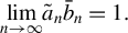 $\underset {n\rightarrow \infty }{\lim }\tilde {a}_n\bar {b}_n=1.$
Thus, according to Lemma 6, we can obtain that
 $$ \begin{align} &\underset{n\rightarrow\infty}{\lim}\ nK_1^{-1}\left(1-F_{\tilde{\eta}_\ell}\left(\tilde{a}_n+\bar{x}\bar{b}_n\right)\right)\nonumber\\ & \quad =\underset{n\rightarrow\infty}{\lim} \frac{1-F_{Z}\left(\tilde{a}_n+\bar{x}\bar{b}_n\right)-\left(F_{\tilde{\eta}_\ell}\left(\tilde{a}_n+\bar{x}\bar{b}_n\right)-F_{Z}\left(\tilde{a}_n+\bar{x}\bar{b}_n\right)\right)}{1-F_{Z}\left(\tilde{a}_n\right)}=e^{-\bar{x}} \end{align} $$
for all
 $\ell \in \mathcal S_0,$
since
 $\tilde {\eta }_\ell $
’s are i.i.d. random variables. It holds that
 $$ \begin{align} \mathrm{P}\left(\underset{\ell\in\mathcal S_0}{\max}\ \tilde{\eta}_\ell\leq\tilde{a}_n+\bar{b}_n\bar{x}\right) &=\mathbb{E}\left(\mathbb{E}\left(\boldsymbol 1_{\left\{\underset{\ell\in\mathcal S_0}{\max}\ \tilde{\eta}_\ell\leq\tilde{a}_n+\bar{b}_n\bar{x}\right\}} \Big | \ \mathcal S_0\right)\right)\nonumber\\ & =\mathbb{E}\left(\left(1-\bar{p}_{n,\bar{x}}\right)^{\text{ card }(\mathcal S_0)}\boldsymbol 1_{\left\{\mathcal{S}_0\neq\unicode{xf8}\right\}}\right), \end{align} $$
where
 $\bar {p}_{n,\bar {x}}=\mathrm {P}\left (\tilde {\eta }_\ell>\tilde {a}_n+\bar {b}_n\bar {x}\right ).$
Since
 $\ln (1-x)\leq -x$
for
 $x\in (0, 1),$
we have
 $$ \begin{align} \left(1-\bar{p}_{n,\bar{x}}\right)^{\text{ card }(\mathcal S_0)}\leq\exp\left(-\text{ card }(\mathcal S_0)\bar{p}_{n,\bar{x}}\right). \end{align} $$
Notice that
 $$ \begin{align*}0\leq\lfloor n/K_1-1\rfloor-\text{ card }(\mathcal S_0)\leq 2N_T,\end{align*} $$
and then by Assumptions 2 and 5, it almost surely holds that
 $$ \begin{align} \frac{\text{ card }(\mathcal S_0)}{n/K_1}\overset{n\rightarrow\infty}{\longrightarrow}1. \end{align} $$
Thus, according to (A.1), we can obtain that almost surely
 $$ \begin{align} \text{ card }(\mathcal S_0)\bar{p}_{n,\bar{x}}\overset{n\rightarrow\infty}{\longrightarrow} e^{-\bar{x}}. \end{align} $$
On the other hand, (A.1) and (A.5) imply that almost surely
 $$ \begin{align} & \left(1-\bar{p}_{n,\bar{x}}\right)^{\text{ card }(\mathcal S_0)}\nonumber\\ &\geq\left(\exp\left(-\text{ card }(\mathcal S_0)\bar{p}_{n,\bar{x}}\right)-\left(1-\underset{\ell\in\mathcal S_0}{\max}\ \bar{p}_{n,\bar{x}}\right)^{\text{ card }(\mathcal S_0)}\left(\exp\left(2\text{ card }(\mathcal S_0)\bar{p}_{n,\bar{x}}^2\right)-1\right)\right)\nonumber\\ & \overset{n\rightarrow\infty}{\longrightarrow}\exp\left(-e^{-\bar{x}}\right), \end{align} $$
where the inequality is due to Lemma 1.3.1 of Galambos (Reference Galambos1978). Now, from (A.3), (A.5), and (A.6), we can see that almost surely
 $$ \begin{align*} \underset{n\rightarrow\infty}{\lim} \ \left(1-\bar{p}_{n,\bar{x}}\right)^{\text{ card }(\mathcal S_0)}=e^{-\bar{x}} \end{align*} $$
as
 $n\rightarrow \infty .$
Then since
 $\left (1-\bar {p}_{n,\bar {x}}\right )^{\text { card }(\mathcal S_0)}< 1,$
by (A.2) and the dominated convergence theorem, we have
 $$ \begin{align} \mathrm{P}\left(\underset{\ell\in\mathcal S_0}{\max}\ \frac{\tilde{\eta}_\ell-\tilde{a}_n}{\bar{b}_n}\leq\bar{x}\right)\overset{n\rightarrow\infty}{\longrightarrow}\exp\left(-e^{-\bar{x}}\right). \end{align} $$
As
 $(\bar {a}_n-\tilde {a}_n)/\bar {b}_n\overset {n\rightarrow \infty }{\longrightarrow } 0$
by Lemma 5, (A.7) implies that
 $$ \begin{align} \mathrm{P}\left(\underset{\ell\in\mathcal S_0}{\max}\ \frac{\tilde{\eta}_\ell-\bar{a}_n}{\bar{b}_n}\leq\bar{x}\right)\overset{n\rightarrow\infty}{\longrightarrow}\exp\left(-e^{-\bar{x}}\right). \end{align} $$
Given Corollary 1, it holds that for any fixed
 $\tilde \epsilon \in (0, \tilde {c}_0-\tilde {c}_2),$
 $$ \begin{align} \mathrm{P}\left(\underset{\ell\in\mathcal S_0}{\max} \ \bar{\eta}_\ell\leq\exp\left(-n^{\tilde\epsilon}\right)\right)\overset{n\rightarrow\infty}{\longrightarrow}1. \end{align} $$
Then we can obtain that for any fixed
 $\epsilon>0, $
 $$ \begin{align*} & \mathrm{P}\left(\underset{\ell\in\mathcal S_0}{\max} \ \left(\eta_\ell-\tilde{\eta}_\ell\right)\geq\epsilon\bar{b}_n \right)=\mathrm{P}\left(\underset{\ell\in\mathcal S_0}{\max} \ \sum_{j=1}^{L_n}\boldsymbol 1_{\left\{0\leq z_{\ell,j}\leq\bar{\eta}_i\right\}}\geq\epsilon\sqrt{L_n}\bar{b}_n/2\right) \\ & \quad\leq \mathrm{P}\left(\underset{\ell\in\mathcal S_0}{\max} \ \sum_{j=1}^{L_n}\boldsymbol 1_{\left\{0\leq z_{\ell,j}\leq\exp\left(-n^{\left(\tilde{c}_0-\tilde{c}_2\right)/2}\right)\right\}}\geq\epsilon\sqrt{L_n}\bar{b}_n/2\right)\\ & \qquad +\mathrm{P}\left(\underset{\ell\in\mathcal S_0}{\max} \ \bar{\eta}_\ell>\exp\left(-n^{\left(\tilde{c}_0-\tilde{c}_2\right)/2}\right)\right)\\ & \quad =\mathrm{P}\left(\underset{\ell\in\mathcal S_0}{\max} \ \sum_{j=1}^{L_n}\boldsymbol 1_{\left\{0\leq z_{\ell,j}\leq\exp\left(-n^{\left(\tilde{c}_0-\tilde{c}_2\right)/2}\right)\right\}}\geq\epsilon\sqrt{L_n}\bar{b}_n/2\right)+o(1). \nonumber \end{align*} $$
By Assumption 6(b), it holds that
 $$ \begin{align*}\mathbb{E}\left( \sum_{j=1}^{L_n}\boldsymbol 1_{\left\{0\leq z_{i,j}\leq\exp\left(-n^{\left(\tilde{c}_0-\tilde{c}_2\right)/2}\right)\right\}}\right)\leq cL_n\exp\left(-n^{\left(\tilde{c}_0-\tilde{c}_2\right)/2}\right).\end{align*} $$
Thus, the Markov inequality and the fact that
 $\text { card }(S_0)=O(n^{1-c_1})$
yield that
 $$ \begin{align*} & \mathrm{P}\left(\underset{\ell\in\mathcal S_0}{\max} \ \sum_{j=1}^{L_n}\boldsymbol 1_{\left\{0\leq z_{\ell,j}\leq\exp\left(-n^{\left(\tilde{c}_0-\tilde{c}_2\right)/2}\right)\right\}}\geq\epsilon\sqrt{L_n}\bar{b}_n/2\right) \\ & \quad\leq \mathbb{E}\left(\text{ card }(\mathcal S_0)\cdot c\sqrt{L_n}\exp\left(-n^{\left(\tilde{c}_0-\tilde{c}_2\right)/2}\right)\bar{b}_n^{-1}\right)\overset{n\rightarrow\infty}{\longrightarrow}0. \end{align*} $$
Then since
 $\eta _\ell \geq \tilde {\eta }_\ell ,$
we have
 $$ \begin{align} \underset{\ell\in\mathcal S_0}{\max} \ \left(\eta_\ell-\tilde{\eta}_\ell\right)=o_{\mathrm{P}}\left(\bar{b}_n\right), \end{align} $$
which completes the proof given (A.8).
COMPETING INTEREST STATEMENT
The author declares that no competing interests exist.
FUNDING STATEMENT
The author acknowledges financial support from the National Natural Science Foundation of China (Grant No. 72103150), and the Project of Construction and Support for High-Level Innovative Teams of Beijing Municipal Institutions (Grant No. BPHR20220119).
SUPPLEMENTARY MATERIAL
Sun, Y. (2025). Supplement to “Randomized testing for jump detection,” Econometric Theory Supplementary Material. To view, please visit: https://doi.org/10.1017/S0266466626100425.