1. Introduction
Mixing and shear dispersion in turbulent flows are important in many natural and industrial processes (Prandtl Reference Prandtl1954; Pope Reference Pope2000). Among the many different types of flow, jets and plumes, which arise from localised sources and which are driven by momentum or buoyancy, are especially intriguing (Turner Reference Turner1979; Carazzo, Kaminski & Tait Reference Carazzo, Kaminski and Tait2008), with applications for modelling volcanic plumes in the atmosphere, hydrothermal plumes in the ocean (Woods Reference Woods2010), effluent spreading in shallow estuaries and river outflows into shallow lakes (Dracos, Giger & Jirka Reference Dracos, Giger and Jirka1992; Daoyi & Jirka Reference Daoyi and Jirka1998). In the latter cases, the flow may be confined, leading to the development of an effectively two-dimensional flow. Dracos et al. (Reference Dracos, Giger and Jirka1992) and Daoyi & Jirka (Reference Daoyi and Jirka1998) have described the motion of two-dimensional jets both experimentally and theoretically, using integral modelling techniques, and have applied this modelling to understand the processes of formation and growth of large eddies in river outflows and the ensuing transport of pollutants in shallow lake environments. As well as modelling the mean properties of the flow, it is of interest to quantify the longitudinal dispersion in such flows, especially if they involve reactions or if chemicals are added to the flow and then become diluted through mixing (Chen & Jirka Reference Chen and Jirka1999; Ai, Law & Yu Reference Ai, Law and Yu2006). Recent experiments measuring the longitudinal dispersion within two-dimensional jets (Landel, Caulfield & Woods Reference Landel, Caulfield and Woods2012a ) suggest that the local turbulent diffusivity is proportional to the product of the local size and speed of the eddies. By adopting this model, accurate predictions of the longitudinal mixing of a dye front, produced by adding a constant flux of dye to an established jet, can be obtained.
In this work we explore the complementary problem of quantifying the mixing in a two-dimensional turbulent plume, driven by a buoyancy flux,
 $f$
. In contrast to a jet, the buoyancy flux causes the momentum flux to increase with distance from the source. We therefore characterise the eddies in such two-dimensional plumes, and explore how they influence the longitudinal dispersion in the flow. Although there have been a number of experiments that explore the dynamics of three-dimensional line plumes produced by a uniform line source of buoyancy, in which the scale of the line source exceeds the vertical scale of the flow (van den Bremer & Hunt Reference van den Bremer and Hunt2014; Paillat & Kaminski Reference Paillat and Kaminski2014), the dynamics of a (confined) two-dimensional turbulent plume is different, as the eddies can only grow in the along- and cross-plume directions (figure 1).
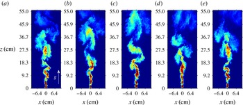
Series of five images illustrating the structure of a two-dimensional plume, and its evolution with time for (a) 15 s, (b) 16 s, (c) 17 s, (d) 18 s and (e) 19 s, using a false colour mapping of concentration to highlight the eddies. As the plume advances from the source, eddies develop which mix with ambient fluid, leading to dilution of the plume fluid. In this experiment
 $s_{0}=17~\text{wt}\%$
and
 $q_{0}=4.4~(\text{cm}^{2}~\text{s}^{-1})$
where
 $s_{0}$
is the initial salinity and
 $q_{0}$
is the initial flux.

First, we describe our experimental system, and present some measurements of both the plume width as a function of distance from the source and the speed of the centre of mass of a dye front. We measure the speed of the leading edge of the eddies in the along-plume direction and explore the variation with position of the product of the frequency and size of the eddies. We use the data to motivate a phenomenological model of the longitudinal dispersion produced by the eddies. We compare the predictions of our model with the dispersion of the dye front in a series of experiments in which a steady flux of dye was added to the source of a steady plume, for
 $t>0$
. We conclude with a discussion of the implications of our work for calculating the residence time distribution of material in a two-dimensional plume, which is key to understanding the rate of dilution by a plume or reactions in which the reaction time is comparable to or longer than the mean travel time through the plume.
2. Experimental observations
We have conducted a series of experiments to measure the mixing produced by two-dimensional turbulent buoyant plumes, in which a finite flux of aqueous saline solution was supplied to a tank of dimensions
 $70~\text{cm}\times 70~\text{cm}\times 1~\text{cm}$
from a localised source of cross-section area
 $0.2~\text{cm}^{2}$
placed at the centre of the top side of the tank. The tank was open on the sides and base and was immersed in a larger reservoir tank, so that plume fluid could leave the tank on reaching the base, and ambient fluid could enter the sides as fluid was entrained by the plume. We carried out a systematic series of experiments in which the aqueous solution that supplied the plume had flow rates in the range
 $1{-}20~\text{cm}^{3}~\text{s}^{-1}$
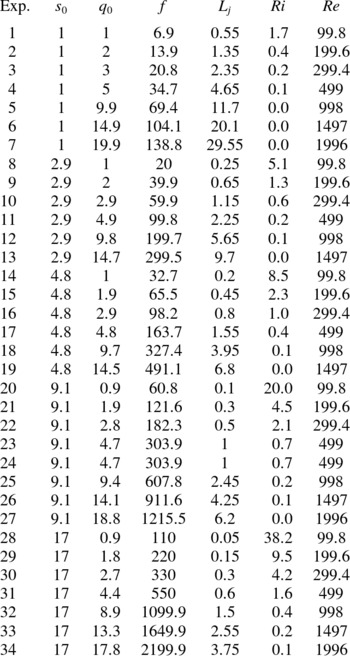
and salinities that ranged from 1 to 17 wt% (table 1). This led to flows with Reynolds numbers of order 100–2000. As shown by Landel, Caulfield & Woods (Reference Landel, Caulfield and Woods2012b
) for such flow rates, the frictional stress on the walls of the tank is small over the vertical extent of the plume, and so to leading order the frictional effects may be neglected.
A summary of the experiments carried out, specifying the initial salt concentration (
 $s_{0}$
), the initial volume and specific buoyancy fluxes per unit length (
 $q_{0}$
and
 $f$
), the jet length (
 $L_{j}$
) and the source Reynolds (
 $\mathit{Re}$
) and Richardson (
 $\mathit{Ri}$
) numbers.

The tank was backlit by an electroluminescent sheet (W&Co LED panel
 $100~\text{cm}\times 60~\text{cm}$
) and the flow was recorded by a 3 Hz series of photographs using a computer-controlled Canon D90 camera in an otherwise dark room. In each experiment, the plume fluid was dyed with a uniform initial intensity of red food dye (
 $3~\text{g}~\text{l}^{-1}$
). Prior to the actual experiment, a series of calibration experiments were carried out in which mixtures of the aqueous saline solution and fresh water were photographed. These were used to generate a calibration curve relating the light intensity recorded by the camera with the dye content and hence the salinity of the fluid. With this calibration, we were able to measure the total salinity of the plume fluid in the tank, and during the course of each experiment this was within 4–5 % of the known supply of salt in the aqueous saline solution.
In figure 1 we present a series of images illustrating the detailed evolving structure of the plume. In this and all subsequent images we show the plume fluid rising from the bottom to the top of the image, as would be the case for a positively buoyant flow. This is for consistency and to help in interpretation with the existing literature (cf. Morton, Taylor & Turner Reference Morton, Taylor and Turner1956; Papanicolaou & List Reference Papanicolaou and List1988). In actual practice the flow was of negatively buoyant aqueous saline solution, and descended to the base of the tank, and so the images are shown upside-down. It may be seen that there are a series of eddies which migrate forward with the flow, growing and mixing as they advance and engulf ambient fluid. In developing a picture of the flow it is useful to consider the time-averaged steady motion in which we assume the eddies entrain ambient fluid at a rate proportional to the mean speed of the eddies (Morton et al.
Reference Morton, Taylor and Turner1956). If the ensemble time-averaged steady plume has speed
 $w(x,z)$
and concentration
 $c(x,z)$
, where
 $x$
is the horizontal position in the plume and
 $z$
is the vertical distance from the source, then we can write the volume flux, specific momentum flux and specific buoyancy flux per unit distance in the
 $y$
direction as
 $$\begin{eqnarray}q=\bar{w}\bar{b}=\int _{-\infty }^{\infty }w\,\text{d}x,\quad m=\bar{w}^{2}\bar{b}=\int _{-\infty }^{\infty }w^{2}\,\text{d}x,\quad f=\bar{g}\bar{w}\bar{b}=\int _{-\infty }^{\infty }wg^{\prime }\,\text{d}x,\end{eqnarray}$$
where
 $w$
is the vertical speed,
 $x$
is the location in the horizontal direction relative to the centreline of the plume,
 $\bar{b}$
is the effective width of the flow,
 $\bar{w}$
is the horizontally averaged vertical speed,
 $g^{\prime }$
is the local buoyancy and
 $\bar{g}$
is the horizontally averaged buoyancy. The local buoyancy
 $g^{\prime }$
is related to the concentration
 $s$
by the relation
 $g^{\prime }=(s/s_{0})g_{0}^{\prime }$
, where
 $g_{0}^{\prime }$
, the buoyancy of the source fluid, is given by
 $g_{0}^{\prime }=({\it\rho}_{j}-{\it\rho}_{e})/{\it\rho}_{e}$
, where
 ${\it\rho}_{j}$
and
 ${\it\rho}_{e}$
are the densities of the aqueous saline solution with concentration
 $s_{0}$
and the environmental fluid. Here,
 $g$
is the acceleration of gravity and
 $s_{0}$
is the concentration of the source fluid. If we assume that the entrainment velocity is proportional to the mean vertical speed,
 ${\it\varepsilon}\bar{w}$
, then the conservation of mass, momentum and buoyancy takes the form (cf. Paillat & Kaminski Reference Paillat and Kaminski2014)
 $$\begin{eqnarray}\frac{\text{d}q}{\text{d}z}=2{\it\varepsilon}\bar{w},\quad m\frac{\text{d}m}{\text{d}z}=kqf,\quad f=\text{const.}=f_{0},\end{eqnarray}$$
where
 $f_{0}$
is the source-specific buoyancy flux and
 $k$
is a constant that depends on the horizontal structure of the ensemble time-averaged velocity and buoyancy. These equations have self-similar solution
 $$\begin{eqnarray}\bar{w}=\left(\frac{kf}{2{\it\varepsilon}}\right)^{1/3},\quad b=2{\it\varepsilon}z,\end{eqnarray}$$
with the buoyancy flux
 $f$
being a constant in a uniform environment (cf. Morton et al.
Reference Morton, Taylor and Turner1956; Paillat & Kaminski Reference Paillat and Kaminski2014). This solution applies once the buoyancy-driven momentum flux, as given by
 $2{\it\varepsilon}z(kf/2{\it\varepsilon})^{2/3}$
, exceeds the initial momentum flux
 $m_{0}$
; this corresponds to points
 $z\gg L_{j}$
, where the jet length
 $L_{j}=m_{0}/(2{\it\epsilon})^{1/3}(kf)^{2/3}$
. For most of the experiments tabulated in table 1, we estimate that
 $L_{j}$
has a value smaller than 15 cm, while the tank is 70 cm deep. Beyond this adjustment region, we expect the ensemble-averaged flow speed to be constant, and the plume width to increase linearly with depth. In fact, in addition to the jet length, in our experimental system, the diameter of the source is one-half of the width of the tank, and so in the immediate vicinity of the source, the plume is three-dimensional; however, within 2–3 cm it evolves into a two-dimensional plume following rapid entrainment and mixing.
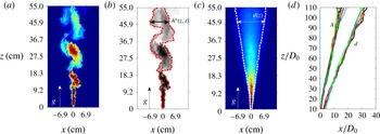
Analysis of the ensemble-averaged concentration of the plume, which is found by averaging over 150 frames from a quasi-steady period of flow corresponding to approximately 50 s (figure 2
c), shows that the horizontal distance
 $d(z)$
over which the concentration falls by a factor
 $e$
scales linearly with height above the source, independently of the buoyancy flux, according to the relation
 $d={\it\lambda}z$
, where
 ${\it\lambda}=0.142\pm 0.016$
(figure 2
d). This result is consistent with values obtained in previous 3D line source plume studies: Kotsovinos & List (Reference Kotsovinos and List1977) found
 ${\it\lambda}=0.13$
while Yih (Reference Yih1977) and Paillat & Kaminski (Reference Paillat and Kaminski2014) report
 ${\it\lambda}=0.15$
.
(a) Photograph of the instantaneous structure of a typical two-dimensional plume, in steady state. (b) Locations of the two bounding lines, defined as the points at which the concentration falls to a value of
 $1/e$
of the maximum concentration on each horizontal line; the distance between these lines is denoted
 $A^{\ast }$
. (c) Time average of 240 frames showing the time-averaged concentration profile. (d) Horizontal distance from the centreline at which the time-averaged concentration has a value of
 $1/e$
times the time-averaged centreline concentration as a function of the distance from the source (d). Also shown is a characteristic cross-plume length scale (A). At each height, this scale is determined by first measuring the horizontal distance between the two points at that height for which the concentration equals
 $1/e$
times the maximum concentration at that level,
 $A^{\ast }$
(b), and then finding a time average of these values. (a–c) Show data for the case
 $q_{0}=4.4~(\text{cm}^{2}~\text{s}^{-1})$
,
 $s_{0}=17~\text{wt}\%$
.

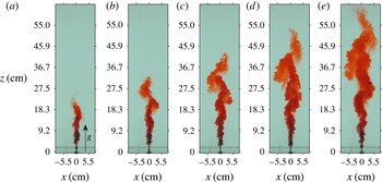
We now explore the role of the eddies in causing the mixing and dispersion within this flow. The nature of the mixing may be seen in the series of photographs of a steady plume shown in figure 3, in which a steady flux of red dye is injected into the source fluid for
 $t>0$
. The red dye is carried forward with the eddies in an irregular fashion, producing a dispersed leading zone of dyed fluid, followed by a more uniformly dyed plume, once the initial spreading front of dye has passed.
Photograph of an evolving two-dimensional line plume, illustrating how red dye, injected into the established steady plume, evolves with time for (a) 1.3 s, (b) 2.3 s, (c) 3.3 s, (d) 4.3 s and (e) 5.3 s. Pictures are shown for the case
 $q_{0}=2.7\,(\text{cm}^{2}~\text{s}^{-1})$
,
 $s_{0}=17~\text{wt}\%$
.

We have measured the horizontal integral of the concentration of the dye in the plume as a function of distance
 $z$
from the source, at a series of times following the introduction of the dye, for 15 of the experiments listed in table 1 (figure 4
a). We have then rescaled the vertical axis by time,
 $z/f^{1/3}t$
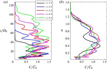
, since we expect the speed of the plume to be a constant. Figure 4(b) illustrates the rescaled profiles. The figure suggests that, beyond the flow adjustment zone near the source, there is a region in which the horizontal integral of the concentration is nearly uniform, noting that the structure of the flow involves a series of eddies which lead to fluctuations of the concentration relative to this uniform value. It also shows that there is a frontal dispersion region in which the horizontally averaged concentration of dye falls back to zero. The rescaled figure 4(b) suggests that the length of this dispersed front also scales with
 $f^{1/3}t$
. We have measured the ensemble average position of the centre of mass of the dispersed front for the 15 experiments, and find that the centre of mass appears to advance with mean speed
 $1.04f^{1/3}$
. We describe the ensemble average of the profiles of the horizontally integrated concentration as a function of the scaled height later in the paper, when modelling the dispersion (figure 7
a), but note here that this mean advection speed is consistent with the horizontally averaged model of the time-averaged plume (2.3).
(a) Experimental data showing the horizontally integrated concentration of dye in the plume as a function of
 $z$
at five times after the start of steady injection of red dye into the plume at
 $t=0$
. (b) Integral of the concentration at different time steps as a function of
 ${\it\eta}=z/(tf^{1/3})$
;
 $q_{0}=4.4~(\text{cm}^{2}~\text{s}^{-1})$
and
 $s_{0}=17~\text{wt}\%$
.

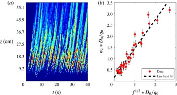
In order to model the dispersion of the dye, relative to the front, we first characterise the properties of the eddies. We have tracked the speed of the front of the eddies as they advance through the tank by constructing a vertical time series along a line close to the centreline (
 $x=3D_{0}$
) of the plume (figure 5
a). This line is shown in false colour to enhance the contrast between the background and the plume fluid which is dyed red at source. The image illustrates that there is a regular series of fronts which migrate through the tank, and that as each front migrates, the colour contrast across the front decreases; these correspond to the leading edges of successive eddies, which mix and become diluted with ambient fluid. The speed of these fronts can be found by using a Hough transform which estimates the gradient of the lines. This suggests that the eddies attain a nearly constant speed within 10 cm of the source, and then advance through the next 50 cm of the tank with a near-constant speed. The procedure has been repeated for a series of experiments with different values of the buoyancy flux
 $f$
(table 1), and in figure 5(b) we show the measured speed of the front of the plume (
 $w_{e}$
) as a function of the buoyancy flux at the source, illustrating that the data collapse to the relation
 $$\begin{eqnarray}w_{e}=(1.3\pm 0.1)f^{1/3}.\end{eqnarray}$$
This value is larger than the speed of the centre of mass of the dye front, as seen in figures 4 and 7(a). This provides the ability for the eddies to disperse the dye longitudinally relative to the centre of mass as they periodically carry dyed fluid beyond the location of the centre of mass, and then mix this dye across the plume. We explore this in the next section.
(a) Time series of the pixels along a vertical line positioned at
 $x=3\times D_{0}$
from the centreline of the plume, shown using false colour, to illustrate the passage of the front of successive eddies. In this experiment,
 $q_{0}=4.4~(\text{cm}^{2}~\text{s}^{-1})$
and
 $s_{0}=17~\text{wt}\%$
. (b) Variation of the speed of the front of the plume (
 $w_{e}$
) for a large number of different buoyancy fluxes, as determined from figures such as 5(a) for
 $x=0$
. The data collapse to the simple relation
 $w_{1}(0,z)\approx 1.30f^{1/3}$
.

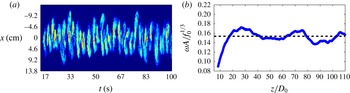
(a) Time series of a horizontal line in the plume (
 $z=42~(\text{cm})$
,
 $q_{0}=4.4~(\text{cm}^{2}~\text{s}^{-1})$
,
 $s_{0}=17~\text{wt}\%$
), using false colour to show how the stream of eddies passes by this line, with successive eddies migrating left or right relative to the source. (b) Time average of the product of frequency and the length scale of the eddies as a function of distance from the source,
 $z$
. Data from one experiment are shown, illustrating how the data collapse to a common limit away from the source (
 $q_{0}=4.4~(\text{cm}^{2}~\text{s}^{-1})$
,
 $s_{0}=17~\text{wt}\%$
).

We now characterise the horizontal fluctuations in the position of the eddies. In figure 6(a), we illustrate a time series showing the variation with time of the concentration of the fluid along a horizontal line through the plume at a distance 42 cm below the source. This false colour image illustrates how, as the plume evolves, the location of successive eddies passing this point oscillates to the left (
 $x>0$
) and right (
 $x<0$
) of the source. Using plots, such as figure 6(a), it was possible to measure the frequency of the passage of the vortices (
 ${\it\omega}$
), by measuring the frequency of the horizontal oscillation of the plume around the centreline. On each horizontal line in the plume, we also measured the horizontal distance
 $A^{\ast }$
between the two points where the concentration of the plume has decreased to a fraction
 $1/e$
of the maximum concentration on that horizontal line (see figure 2
a,b), at a specific time instant. We then find a time average of
 $A^{\ast }$
, defined as
 $A(z)$
, for each value of the vertical distance
 $z$
from the source. Figure 2(d) shows the variation of
 $A$
as a function of
 $z$
. It is seen that
 $A$
is considerably smaller than
 $d$
, the width of the ensemble time-averaged flow (figure 2
d). This reflects the difference between the actual dilution of the fluid, as measured by
 $A$
, and the width of the time-averaged concentration field
 $d$
, which captures the combined effect of the dilution plus the horizontal oscillation of the position of the flow. If the horizontal variation of concentration, relative to the centre of the plume, and the position of the centre of the plume, relative to the centre of the tank, both follow a normal distribution, with variance
 ${\it\sigma}_{A}$
and
 ${\it\sigma}_{0}$
, then the variance of the joint distribution,
 ${\it\sigma}_{d}$
, is the sum of the variance of each distribution,
 ${\it\sigma}_{d}={\it\sigma}_{0}+{\it\sigma}_{A}$
, with the e-folding distances given by
 $\sqrt{{\it\sigma}_{A}}$
, for the actual dilution of the fluid, and
 $\sqrt{{\it\sigma}_{d}}$
, for the time-averaged concentration field. Given the e-folding distances
 $d\sim 0.28z$
and
 $A\sim 0.14z$
(figure 2
d), it follows that
 ${\it\sigma}_{0}\approx 3{\it\sigma}_{A}$
, so the variance in concentration associated with the oscillations is approximately three times that of the actual dilution.
Since the plume flow is essentially composed of the eddies, we expect that the frequency of the eddies passing this horizontal level,
 ${\it\omega}$
, times their characteristic length scale,
 $A$
, should scale with the mean speed of the flow. Since the speed is a constant proportional to
 $f^{1/3}$
(figures 4
b, 5
a), we anticipate that
 ${\it\omega}A$
will be independent of distance from the source. We have also measured the eddy frequency,
 ${\it\omega}$
, at each horizontal surface in the plume, and combining this with the measurement of
 $A$
, in figure 6(b) we illustrate the value of
 ${\it\omega}A/f^{1/3}$
as a function of the distance from the source. Similar data have been collected for experiments with different buoyancy fluxes (table 1), and suggest that, beyond a flow adjustment zone which extends over a region of approximately 15 cm ahead of the source, the quantity
 ${\it\omega}A/f^{1/3}\sim 0.16\pm 0.01$
, This result is also consistent with dimensional analysis. From the data presented in figures 5 and 6, we can now envisage how the eddies lead to the longitudinal dispersion of the dye front seen in figures 3 and 4.
3. Model of the dispersive mixing
We now model the influence of the dispersive mixing on the horizontal integral of concentration along the plume by assuming that the mixing is produced by interaction of the time-dependent eddies with the mean flow. Using the results relating to the speed, frequency and length scale of the eddies, and adopting concepts from classical models of mixing length theory (Prandtl Reference Prandtl1925) and turbulent dispersion (Taylor Reference Taylor1954), we expect that over time scales long compared with the eddy turnover time, the eddies lead to an effective dispersivity that scales as
 $z\,f^{1/3}$
, where
 $z$
is the distance downstream. We can then hypothesise that the horizontal integral
 $C(z,t)=\int _{-\infty }^{\infty }c(x,z,t)\,\text{d}x$
of the ensemble-averaged concentration evolves according to the phenomenological conservation law
 $$\begin{eqnarray}\frac{\partial C}{\partial t}+{\it\alpha}f^{1/3}\frac{\partial C}{\partial z}=\frac{\partial }{\partial z}\left({\it\beta}zf^{1/3}\frac{\partial C}{\partial z}\right),\end{eqnarray}$$
where
 ${\it\beta}$
is a constant of proportionality for the turbulent dispersion and
 ${\it\alpha}$
is the constant that determines the mean speed of the dye front. By comparing the solutions of this equation with our experimental data (figure 4), we now estimate values for
 ${\it\alpha}$
and
 ${\it\beta}$
.
Equation (3.1) can be used to describe the advance of a front of dye within a steady plume of buoyancy flux
 $f$
. If there is a flux of dye
 $Q_{c}$
released into the plume at
 $z=0$
for
 $t\geqslant 0$
, then the horizontally averaged concentration may be written as
 $$\begin{eqnarray}C(z,t)=\frac{Q_{c}}{f^{1/3}}\mathscr{H}\left(\frac{z}{f^{1/3}t}\right),\end{eqnarray}$$
where
 ${\it\eta}=z/(f^{1/3}t)$
and
 $\mathscr{H}$
satisfies the relation
 $$\begin{eqnarray}-\!{\it\eta}\frac{\text{d}\mathscr{H}}{\text{d}{\it\eta}}+{\it\alpha}\frac{\text{d}\mathscr{H}}{\text{d}{\it\eta}}={\it\beta}\frac{\text{d}}{\text{d}{\it\eta}}\left({\it\eta}\frac{\text{d}\mathscr{H}}{\text{d}{\it\eta}}\right),\end{eqnarray}$$
and the expression for the global conservation of dye
 $$\begin{eqnarray}\int _{0}^{\infty }\mathscr{H}({\it\eta})\,\text{d}{\it\eta}=1.\end{eqnarray}$$
This leads to the solution
 $$\begin{eqnarray}\mathscr{H}({\it\eta})=\frac{\displaystyle \int _{{\it\eta}}^{\infty }{\it\zeta}^{({\it\alpha}/{\it\beta})-1}\exp \displaystyle \left(-\frac{{\it\zeta}}{{\it\beta}}\right)\,\text{d}{\it\zeta}}{\displaystyle \int _{0}^{\infty }{\it\zeta}^{{\it\alpha}/{\it\beta}}\exp \displaystyle \left(-\frac{{\it\zeta}}{{\it\beta}}\right)\,\text{d}{\it\zeta}}=\frac{{\it\Gamma}\displaystyle \left(\frac{{\it\alpha}}{{\it\beta}},\frac{{\it\eta}}{{\it\beta}}\right)}{{\it\Gamma}\displaystyle \left(\frac{{\it\alpha}}{{\it\beta}}+1,0\right)},\end{eqnarray}$$
where we require that
 $\mathscr{H}\rightarrow 0$
as
 ${\it\eta}\rightarrow \infty$
, and
 ${\it\Gamma}(a,b)$
is the incomplete Gamma function.
We have compared the solution (3.5) for the horizontally integrated concentration with our experimental data in which a steady flux of dye is added to an established plume at
 $t=0$
. As the dye spreads downstream, we have measured the horizontal integral of concentration as a function of the scaled distance
 $z/f^{1/3}t$
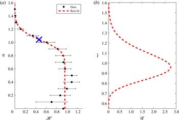
(figure 4; table 1). By taking the ensemble average of 15 experiments, we estimate that the best-fit model (3.5) corresponds to the parameters
 ${\it\alpha}=1.04\pm 0.11$
and
 ${\it\beta}=(2.01\pm 0.25)\times 10^{-2}$
(figure 7
a), where
 ${\it\alpha}f^{1/3}$
corresponds to the speed of the centre of mass of the front, and
 ${\it\beta}f^{1/3}z$
to the dispersivity relative to this point.
(a) Mean integral of the concentration obtained by averaging the mean integral concentrations of 15 experiments as a function of
 $z/(tf^{1/3})$
; the position of the centre of mass has been identified with a blue cross. (b) Variation of the horizontally averaged concentration as a function of time, passing the point
 $z_{0}=1$
, which results from an instantaneous release of a finite mass of tracer at
 $z=0$
, as obtained from (3.9).

Using this model, we can also find the residence time distribution of a finite pulse of dye added to the system at
 $t=0$
(Danckwerts Reference Danckwerts1953); the residence time distribution provides information about the variation with time of the horizontally averaged concentration of the tracer passing a horizontal plane above the source. Such information can be key to modelling the products of chemical reactions in the plume produced, especially when the reaction time is comparable to the travel time through the plume, so that the distribution of travel times lead to different degrees of partial reaction. With a point release of tracer of finite mass
 $V_{c}$
(per unit distance in the y direction), the horizontal integral of concentration follows a solution of the form
 $$\begin{eqnarray}C(z,t)=\left(\frac{V_{c}}{f^{1/3}t}\right)\mathscr{G}({\it\eta}),\end{eqnarray}$$
where the global conservation of mass requires
 $$\begin{eqnarray}\int _{0}^{\infty }\mathscr{G}({\it\eta})\,\text{d}{\it\eta}=1,\end{eqnarray}$$
and
 $\mathscr{G}\rightarrow 0$
as
 ${\it\eta}\rightarrow 0$
. With these conditions,
 $\mathscr{G}({\it\eta})$
satisfies the equation
 $$\begin{eqnarray}-\!\frac{\text{d}}{\text{d}{\it\eta}}({\it\eta}\mathscr{G})+{\it\alpha}\frac{\text{d}}{\text{d}{\it\eta}}\mathscr{G}={\it\beta}\frac{\text{d}}{\text{d}{\it\eta}}\left({\it\eta}\frac{\text{d}}{\text{d}{\it\eta}}\mathscr{G}\right)\end{eqnarray}$$
and has solution
 $$\begin{eqnarray}\mathscr{G}({\it\eta})=\frac{[{\it\eta}^{{\it\alpha}/{\it\beta}}\exp (-{\it\eta}/{\it\beta})]}{\left[\displaystyle \int _{0}^{\infty }{\it\eta}^{{\it\alpha}/{\it\beta}}\exp (-{\it\eta}/{\it\beta})\,\text{d}{\it\eta}\right]}=\frac{[{\it\eta}^{{\it\alpha}/{\it\beta}}\exp (-{\it\eta}/{\it\beta})]}{{\it\beta}^{{\it\alpha}/({\it\beta}+1)}{\it\Gamma}\displaystyle \left(\frac{{\it\alpha}}{{\it\beta}}+1\right)}.\end{eqnarray}$$
If an observer at position
 $z_{0}$
records the concentration with time, then the distribution of horizontally integrated concentration passing
 $z_{0}$
has the time dependence
 $C(z_{0},t)$
, as illustrated in figure 7(b) as a function of the dimensionless time
 $\hat{t}=tf^{1/3}/z_{0}$
. The mean time,
 ${\it\tau}$
, and the variance in time,
 ${\it\sigma}$
, of the concentration pulse passing
 $z_{0}$
are given by
 $$\begin{eqnarray}{\it\tau}=\frac{\displaystyle \int _{0}^{\infty }tC(z_{0},t)\,\text{d}t}{\displaystyle \int _{0}^{\infty }C(z_{0},t)\,\text{d}t},\quad {\it\sigma}=\frac{\displaystyle \int _{0}^{\infty }t^{2}C(z_{0},t)\,\text{d}t}{\displaystyle \int _{0}^{\infty }C(z_{0},t)\,\text{d}t}-{\it\tau}^{2}.\end{eqnarray}$$
Using the values for
 ${\it\alpha}$
and
 ${\it\beta}$
based on our experimental data, we then find that the dimensionless mean residence time is approximately 1.0 and the dimensionless standard deviation
 $\sqrt{{\it\sigma}}\sim 0.15{\it\tau}$
. In dimensional variables, the mean residence time and standard deviation in residence time at a point
 $z_{0}$
then have the values
 $z_{0}/f^{1/3}$
and
 $0.15z_{0}/f^{1/3}$
.
4. Discussion
In this paper we have investigated mixing within a two-dimensional turbulent plume confined between two parallel plates. The flow is controlled by the dynamics of large eddies which form in the plume and migrate downstream, stirring and mixing ambient fluid into the plume. We have explored the turbulent dispersion produced by these meandering eddies. By parameterising the mixing of the horizontally averaged concentration of tracer in terms of a longitudinal dispersion coefficient, which depends on the length scale and speed in the flow,
 $0.02f^{1/3}z$
, we have been able to formulate a model for the mixing. This has been tested with experimental data for the horizontal integral of concentration, and in the case that a steady flux of dye is added to a steady plume at
 $t=0$
, the advance of the dispersing dye front is well modelled by our phenomenological relation.
In developing models of reacting plumes in which the reactions may be passive, or may in fact generate buoyancy, for example through the release of thermal energy or production of small bubbles or particulate, quantification of the longitudinal mixing may be key. Equation (3.10) leads to a prediction of the residence time distribution of a passive tracer carried by the plume: the model shows that the standard deviation in the residence time may be a fraction 0.15 of the mean.