1. Introduction
The manipulation and optimization of jets have always attracted attention in the field of flow control. According to different external conditions, the major investigations of jets can be divided into two broad categories: jets in quiescent condition (i.e. free jets) and jets in cross-flow (JICF). Compared to free jets, JICF complicate the flow-field features by interaction with the cross-flow. As documented in extensive research, the flow field of a circular steady jet issued into a cross-flow can form a complex set of vortical structures, including counter-rotating vortex pairs, windward and leeward shear-layer vortices, upstream horseshoe vortices and upright wake vortices (Margason Reference Margason1993; Fric & Roshko Reference Fric and Roshko1994; Kelso, Lim & Perry Reference Kelso, Lim and Perry1996). Based on the relevant flow physics, JICF are better at entrainment and mixing than free jets (Mahesh Reference Mahesh2013), and therefore are widely used in engineering and environmental control systems, such as fuel injection in gas-turbine combustors, film cooling of turbine blades, thrust vector control of high-speed vehicles, industrial mixing and pollutant dispersion (Smith & Mungal Reference Smith and Mungal1998; New, Lim & Luo Reference New, Lim and Luo2003; Mahesh Reference Mahesh2013).
The trend towards lower energy consumption in aerodynamics has promoted active or passive flow control techniques to further improve the control efficiency of jets. Synthetic jets (Smith & Glezer Reference Smith and Glezer1998; Glezer & Amitay Reference Glezer and Amitay2002) are effective in actively controlling vortex generation through periodically oscillating the fluid in a working system. Holman et al. (Reference Holman, Utturkar, Mittal, Smith and Cattafesta2005) studied the formation criteria for synthetic jets, namely that the reciprocal of the Strouhal number must be larger than 0.16 and 1 for circular and two-dimensional (2-D) synthetic jets, respectively. On that condition, a strong synthetic jet can form trains of discrete vortical structures, which transfer momentum into the external environment to modify aerodynamic shape (DeMauro, Leong & Amitay Reference DeMauro, Leong and Amitay2013; Feng & Wang Reference Feng and Wang2014), or to delay or suppress flow separation (Zhang & Zhong Reference Zhang and Zhong2011; Tang et al. Reference Tang, Salunkhe, Zheng, Du and Wu2014).
For synthetic jets in quiescent condition, two main dimensionless parameters, Reynolds number (Re) and dimensionless stroke length (L), are used to determine the flow state of vortical structures, and their motion distance from the jet exit in one cycle, respectively. Research on circular or 2-D synthetic jets has manifested increased near-field entrainment and spreading rates in comparison with steady jets (Cater & Soria Reference Cater and Soria2002; Smith & Swift Reference Smith and Swift2003). With the merits of compact size and low cost of manufacture, synthetic jets in cross-flow have shown potential applications in the flow control community. A series of studies have been implemented to reveal the flow physics.
Crook & Wood (Reference Crook and Wood2001) studied a cylinder with an array of circular synthetic jets in a cross-flow. The results showed tilting and stretching of vortex rings. In addition, a well-defined streamwise vortex pair was observed immediately downstream of each jet orifice to interact with the separated flow. Zhong, Millet & Wood (Reference Zhong, Millet and Wood2005) utilized dye flow visualization to investigate the behaviour of circular synthetic jets with ReL (based on stroke length) from 16 to 245, L from 0.56 to 1.4 in a laminar boundary layer at velocity ratio (VR) from 0.06 to 0.7. The vortical structures exhibited three types with increased L and VR: hairpin vortices, stretched vortex rings, and tilted and distorted vortex rings. As a continuous work, Jabbal & Zhong (Reference Jabbal and Zhong2008) established the dimensionless parameter space of the above three vortical structures. They found an upper limit of VR = 0.4 for both hairpin vortices and stretched vortex rings, the thermal footprints of which produced two streaks of high surface heat transfer downstream of the orifice. Conversely, only a single streak of high surface heat transfer could be observed for tilted and distorted vortex rings. Similar to the flow pattern of the 2-D circular cylinder model in Crook & Wood (Reference Crook and Wood2001), either hairpin vortices or stretched vortex rings could be responsible for delaying flow separation.
To understand the underlying flow mechanism, Zhou & Zhong (Reference Zhou and Zhong2009) and Jabbal & Zhong (Reference Jabbal and Zhong2010) used three-dimensional (3-D) numerical simulation and 2-D particle image velocimetry (PIV) to study the flow fields of the above three vortical structures. Hairpin vortices and stretched vortex rings exhibited the characteristics of a streamwise vortex pair embedded in the boundary layer with a common upwash, while tilted and distorted vortex rings induced a tertiary streamwise vortex pair in the near-wall region with a common downwash. By measuring the wall shear stress, stretched vortex rings were found to offer the best performance of higher near-wall fluid mixing, persistency and lower spatial fluctuations. Other works have focused on the operation condition, e.g. actuator location and frequency of circular (Lardeau & Leschziner Reference Lardeau and Leschziner2011; Zhang & Zhong Reference Zhang and Zhong2011) and 2-D slot (Dandois, Garnier & Sagaut Reference Dandois, Garnier and Sagaut2007) synthetic jets on reducing the size of the separated region for a turbulent boundary layer separating from a ramp.
Recently, flow control with synthetic jets from non-circular orifices has been popular due to their enhanced entrainment and mixing compared to circular and 2-D synthetic jets. The main mechanism can be attributed to axis switching of non-circular vortex rings, i.e. the major axis and minor axis of vortex rings are interchanged relative to their initial orientations due to azimuthal non-uniform shear-layer curvature (Gutmark & Grinstein Reference Gutmark and Grinstein1999; Grinstein Reference Grinstein2001). Rectangular configurations are of particular interest by virtue of their wide applications in aviation and industry. Based on the orifice aspect ratio (AR), the investigations of rectangular synthetic jets involve two classes: high aspect ratio (AR > 5) and low aspect ratio (AR ≤ 5). The works of Amitay & Cannelle (Reference Amitay and Cannelle2006), Kotapati, Mittal & Cattafesta (Reference Kotapati, Mittal and Cattafesta2007), Van Buren, Whalen & Amitay (Reference Van Buren, Whalen and Amitay2014) and Van Buren & Amitay (Reference Van Buren and Amitay2016) can provide sufficient understanding of the flow structures and flow-field characteristics for high-AR rectangular synthetic jets in quiescent condition.
In terms of interaction with a cross-flow, Smith (Reference Smith2002) carried out a wind-tunnel experiment of an AR = 45 rectangular synthetic jet actuator array in a turbulent boundary layer at VR = 1.2. He examined two orifice orientations, with the rectangular long side normal to and aligned with the cross-flow direction, respectively. The boundary layer of the former developed a wake-like region due to the blockage effect, while the latter formed streamwise vortices embedded within the boundary layer. However, it is difficult to understand how the flow structures influence the boundary layer from the measurements by hot-wire anemometry. Ravi, Mittal & Najjar (Reference Ravi, Mittal and Najjar2004) focused on interactions of square, and AR = 2 and 4 rectangular synthetic jets with a cross-flow using 3-D numerical simulations; however, the details on the evolution of vortical structures cannot be obtained from the limited results. Van Buren et al. (Reference Van Buren, Beyar, Leong and Amitay2016a) used stereoscopic PIV to study AR = 6, 12 and 18 rectangular synthetic jets normally issued into a laminar boundary layer at VR = 0.5, 1 and 1.5. The flow fields were characterized by a recirculation region downstream of the orifice and a steady streamwise vortex pair farther downstream, akin to the findings in Smith (Reference Smith2002). In addition, the virtual blockage of the jet was reduced with the decreased AR. In another similar study, Van Buren et al. (Reference Van Buren, Beyar, Leong and Amitay2016b) investigated the orifice orientation with pitch (20°−90°) and skew (0°−90°) angles on the vortex formation of an AR = 18 rectangular orifice. Three types of scenarios, i.e. no coherent vortices, a singular strong streamwise vortex or a symmetric streamwise vortex pair, were detected for different combinations of the orifice skew and pitch angles. The orifice with larger pitch and smaller skew angles caused higher blockage, and thus a stronger velocity deficit in the free stream.
From the above, the flow structures for rectangular synthetic jets in cross-flow exhibit some differences from those for circular ones, suggesting an important role of the orifice configuration in flow control effectiveness. Most of the existing studies pertain to high-AR (AR > 5) synthetic jets; however, the interactions of low-AR (AR ≤ 5) ones with a cross-flow have rarely been reported. The recent works of Wang et al. (Reference Wang, Feng, Wang and Li2018), Shi, Feng & Wang (Reference Shi, Feng and Wang2019) and Wang, Feng & Xu (Reference Wang, Feng and Xu2019) have demonstrated significant entrainment and mixing enhancement for low-AR non-circular synthetic jets in quiescent condition associated with axis switching and streamwise vortices. Therefore, low-AR rectangular synthetic jets in cross-flow are worth studying in detail to achieve better flow control applications.
This paper aims to explore the fundamental interactions between low-AR rectangular synthetic jets and a cross-flow. The focus is to analyse the impact of the orifice orientation on the evolution of the flow structures and the relevant flow physics. For this purpose, two different orifice orientations relative to the cross-flow direction were investigated for an AR = 3 rectangular orifice. Note that this aspect ratio was selected considering that AR = 3 displayed superior entrainment performance for rectangular free synthetic jets with ARs from 1 to 5 (Wang et al. Reference Wang, Feng, Wang and Li2018). In addition, tomographic PIV measurement was performed to characterize the flow field three-dimensionality. It is hoped that the current results are helpful for understanding the mechanism by which low-AR non-circular synthetic jets influence control.
2. Experimental set-up and methodology
2.1. Experimental facility
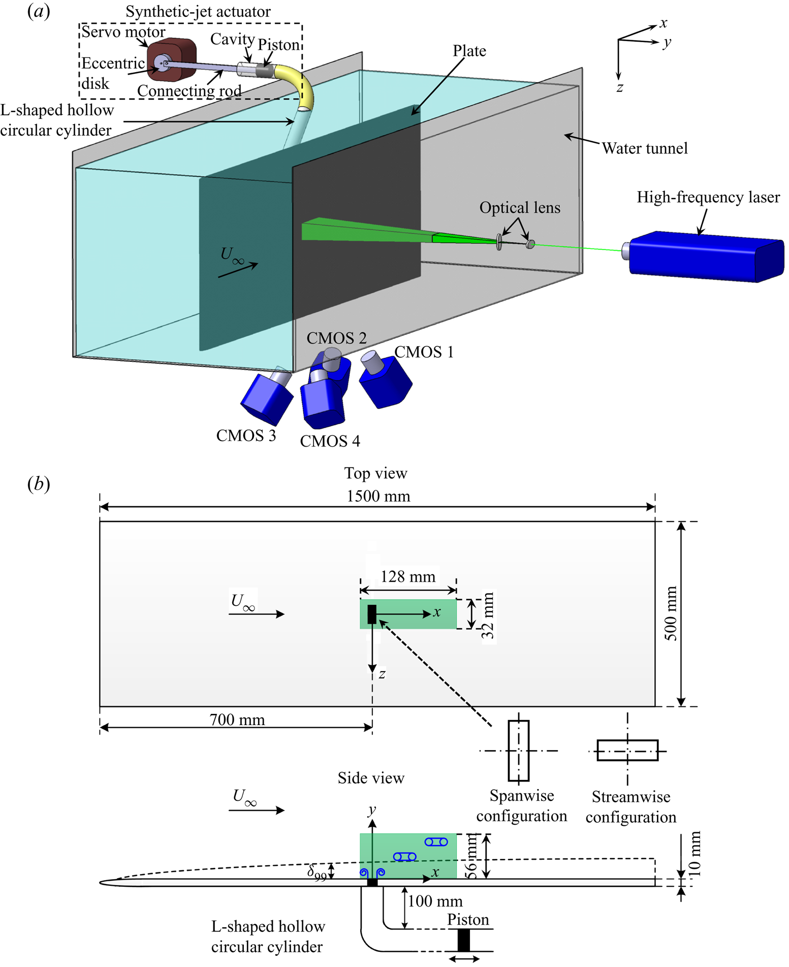
The experiments were conducted in a recirculation water tunnel (Zhu et al. Reference Zhu, Wang, Wang and Wang2017) with a Plexiglas test section of 3000 mm (length) × 700 mm (width) × 600 mm (height). The maximum free-stream velocity in the test section could be up to 0.5 m s−1 with the turbulence level no more than 0.8 %. The synthetic jet actuator in this investigation was a piston-type one, as shown by the dashed box in figure 1(a). The length of the connecting rod was lc = 300 mm, and the diameter of the piston was Dp = 29 mm. The synthetic jet actuator was connected with an L-shaped hollow circular cylinder to horizontally generate synthetic jets underwater. Note that the horizontal section of the L-shaped cylinder was 100 mm, and that was long enough to avoid the impact of the bent part on the formation of synthetic jets. A detailed introduction to this synthetic jet device could be found in Feng & Wang (Reference Feng and Wang2010) and Xu et al. (Reference Xu, Wang, Feng, He and Wang2018). The end of the L-shaped cylinder was flush-mounted in a plate with the jet orifice. The plate was mounted vertically to the bottom of the test section, and the cross-flow direction was parallel to the plate surface.
(a) Isometric schematic view of experimental set-up for tomographic PIV in the test section of the water tunnel. (b) Top and side views of the plate in (a), and spanwise and streamwise configurations of the AR = 3 rectangular orifice.

During the experiments, the water height was kept at 550 mm, and the temperature was 26 ± 0.2 °C. The plate was made of anodized aluminium with 1500 mm (length) × 500 mm (width) × 10 mm (thickness), and this gave a blockage ratio of approximately 1.3 %. The leading edge of the plate was modified to be a 1 : 5 elliptic shape to minimize flow separation and boundary-layer transition. Two AR = 3 rectangular configurations with different orientations were investigated in this study. The rectangular long side was normal to, and aligned with, the free-stream direction, namely spanwise and streamwise configurations, respectively (figure 1b). The circular equivalent diameter of the orifice was De = 8 mm. The position of the jet orifice was 700 mm (87.5De) away from the leading edge of the plate. The plate surface was 400 mm (50De) away from the sidewall of the test section, which could guarantee less wall influence on the investigated field in the wall-normal direction. The coordinate system was defined such that the origin was located at the centre of the jet orifice with the x-axis along the free-stream direction, y-axis normal to the plate and z-axis along the spanwise direction.
2.2. Synthetic jet and cross-flow parameters
Throughout the experiments, the servo electromotor of the synthetic jet actuator was controlled by a constant sinusoidal wave signal, and the excitation frequency and amplitude of the synthetic jet actuator were fixed at fe = 2 Hz (the excitation cycle T = 1/fe = 0.5 s) and Ae = 1.38 mm. The circular equivalent diameter was used as the characteristic length by referring to the previous non-circular jet study (Gutmark & Grinstein Reference Gutmark and Grinstein1999). The instantaneous velocity at the jet exit u(t) can be simplified as follows based on mass conservation of the incompressible flow when  ${l_c} \gg {A_e}\textrm{ }({{A_e}/{l_c} = 0.0046} )$:
 \begin{equation}u(t) \approx 2{\rm \pi} {A_e}{f_e}{({D_p}/{D_e})^2}\sin (2{\rm \pi} {f_e}t).\end{equation}
The averaged velocity at the jet exit U 0 is expressed as follows (Smith & Glezer Reference Smith and Glezer1998; Glezer & Amitay Reference Glezer and Amitay2002), i.e. the time-averaged blowing velocity over the entire cycle:
 \begin{equation}{U_0} = \frac{1}{T}\int_0^{T/2} {u(t)\,\textrm{d}t} = 2{A_e}{f_e}{({D_p}/{D_e})^2}.\end{equation}
Thus U 0 = 72.5 mm s−1, and the two main dimensionless parameters of the synthetic jet, Reynolds number was  $R{e_{{U_0}}} = 664$ and dimensionless stroke length was L = 4.5, defined as
 \begin{gather}R{e_{{U_0}}}\; = {U_0}{D_e}/\nu ,\end{gather}
 \begin{gather}L = {L_0}/{D_e}_{} = {U_0}T/{D_e},\end{gather}
where ν is the kinematic viscosity of water, and L 0 is the stroke length.
The free-stream velocity over the plate in the test section was  ${U_\infty } = 71.3 \pm 0.8\;\textrm{mm}\;{\textrm{s}^{ - 1}}$, and thus the synthetic-jet to free-stream velocity ratio
 $\textrm{VR} = {U_0}/{U_\infty } \approx 1$. This velocity ratio was used so as to compare the current results with previous studies for high-AR rectangular synthetic jets (Van Buren et al. Reference Van Buren, Beyar, Leong and Amitay2016a,Reference Van Buren, Beyar, Leong and Amitayb) under the same velocity ratio. Near the wall, the maximum streamwise velocity fluctuation upstream of the orifice did not exceed 4 % of the free-stream velocity, indicating the current noise level. The boundary-layer thickness
 ${\delta _{99}}$ at the jet exit was 16.12 mm (2.02De) determined by 99 %
 ${U_\infty }$ corresponding to the free-stream Reynolds number of
 $R{e_{{\delta _{99}}}} = 1317$. The boundary-layer shape factor is computed as
 \begin{equation}H = \; \frac{{{\delta ^\ast }}}{\theta } = \frac{{\int_0^\infty {\left( {1 - \frac{{{U_x}}}{{{U_\infty }}}} \right)\,\textrm{d}y} }}{{\int_0^\infty {\frac{{{U_x}}}{{{U_\infty }}}\left( {1 - \frac{{{U_x}}}{{{U_\infty }}}} \right)\,\textrm{d}y} }},\end{equation}
where  ${\delta ^\ast }$ and
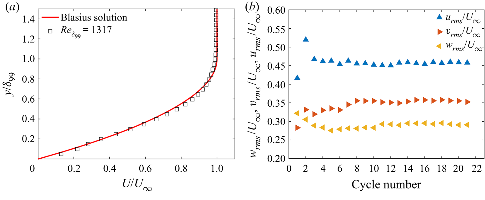
 $\theta $ denote the displacement thickness and the momentum thickness, respectively. At the jet exit, H was 2.60, indicating the laminar flow regime in the boundary layer. The comparison of the undisturbed velocity profile at the jet exit with the theoretical Blasius solution is shown in figure 2(a). Relevant parameters of the synthetic jet and boundary layer are summarized in table 1.
(a) Comparison of undisturbed boundary-layer velocity profile at the jet exit with the theoretical Blasius solution. (b) Normalized velocity fluctuations  ${u_{rms}}/{U_\infty }$,
 ${v_{rms}}/{U_\infty }$ and
 ${w_{rms}}/{U_\infty }$ at the vortex core near the jet exit versus cycle number for the spanwise case.

Major parameters of synthetic jet and boundary layer at the jet exit.

2.3. Tomographic particle image velocimetry measurements
Time-resolved tomographic PIV was applied to measure the 3-D velocity fields of rectangular synthetic jets interacting with a cross-flow (figure 1a). For comparison, the 3-D velocity field of a rectangular synthetic jet issued into a quiescent environment was also measured; and note that the y-axis corresponds to the streamwise direction for the free case. Hollow glass beads with diameters in the range of 5–20 μm and density of 1.05 g cm−3 were seeded to a particle image density of 0.05 particles per pixel. A high-frequency double-pulsed solid-state laser (Vlite-Hi-30k, 532 nm wavelength, 2 × 30 mJ pulse−1 at 1 kHz) was used to produce the volumetric illumination source perpendicular to the plate through a combination of two optical lenses. The width of the volumetric illumination source and its location relative to the orifice centre in the x-axis direction were adjusted according to the cases with and without cross-flow.
Four high-speed complementary metal oxide semiconductor (CMOS) cameras (Photron Fastcam SA2/86K-M3) equipped with 85 mm Nikon lenses at f/11 were distributed under the bottom of the test section to capture the particle images in the investigated field (figure 1a). The viewing angle between CMOS 1 and CMOS 4 (CMOS 2 and CMOS 3) was approximately 60°, and that between CMOS 1 and CMOS 2 (CMOS 3 and CMOS 4) was approximately 30°. The distance between the lens and the measurement domain was around 700 mm, corresponding to a focus depth of 40 mm, guaranteeing the recording of all the particles in the measurement volume in focus. Before the experiment, the cameras, laser and data acquisition system were accurately synchronized by a synchronous controller. Each camera resolution was set to 2048 (x) × 1024 (y) pixels for the cases in cross-flow, and to 1024 (x) × 2048 (y) pixels for the free case.
The sequences of particle images were captured at 1 kHz ( $ {\rm \Delta} t = 0.001 $ s). A pair of particle images with the interval of
 $ 3{\rm \Delta} t $ was used to calculate each velocity vector field. By doing this, the maximum particle displacement between adjacent frames was less than 10 pixels. In total, 10 914 particle images were recorded after the jet flow was adequately steady. To save calculation time, 50 instantaneous velocity fields were reserved in each excitation cycle, and thus the actual time resolution was 100 Hz (50 times the excitation frequency), which could effectively resolve the vortex dynamics. Using the spanwise configuration as an example, we performed a convergence examination of the velocity fluctuations at the vortex core near the jet exit (figure 2b). The results showed that the variation level of all the velocity fluctuations was less than 1 % of the free-stream velocity after the cycle number of 8. This result could meet the current comparable analysis of the flow fields of different orifice orientations.
In image preprocessing, after background subtraction and Gaussian smoothing with a grid size of 3 × 3 pixels, volume self-calibration was implemented to improve the accuracy of the mapping function (Wieneke Reference Wieneke2008) to achieve the reduction of the original disparity error to less than 0.1 pixel. Using the self-calibrated mapping function, the 3-D particle intensity distribution was reconstructed following the MART algorithm (Elsinga et al. Reference Elsinga, Scarano, Wieneke and van Oudheusden2006). The measurement volume size was 128 mm (x) × 56 mm (y) × 32 mm (z) (16De × 7De × 4De) for the cases in cross-flow (figure 1b), and 60 mm (x) × 104 mm (y) × 32 mm (z) (7.5De × 13De × 4De) for the free case, respectively. The digital image resolution was 14.3 pixels mm−1 corresponding to the resolution of 13.2 voxels mm−1 in the object space. The 3-D vector field was calculated by an iterative cross-correlation algorithm with multi-grid and window deformation (Scarano & Riethmuller Reference Scarano and Riethmuller2000), and the final interrogation volume size was 48 × 48 × 48 voxels with 75 % overlap. Then the space resolution was 3.64 mm (0.46De) and the vector spacing was 0.91 mm (0.11De) in each direction, enabling the large-scale vortical structures to be resolved in this study. The resulting 3-D vector field was spatially filtered using a divergence-free smoothing algorithm (Wang et al. Reference Wang, Gao, Wang, Wei and Wang2016).
The experimental uncertainty is mainly attributed to the entire data size and the cross-correlation analysis of PIV. Specifically, the uncertainties in the mean velocity and velocity fluctuation can be estimated as (Ye, Schrijer & Scarano Reference Ye, Schrijer and Scarano2016)
 \begin{gather} {\varepsilon _u} = \frac{{{\sigma _u}}}{{\sqrt N }},\end{gather}
 \begin{gather}{\varepsilon _{{u_{rms}}}} = \frac{{{\sigma _u}}}{{\sqrt {2(N - 1)} }},\end{gather}
where  ${\sigma _u}$ is the typical level of normalized streamwise velocity fluctuations, and N is the number of uncorrelated samples. In this study, the maximum of the normalized streamwise velocity fluctuation is less than 0.6, corresponding to the maximum of
 ${\varepsilon _u}$ and
 ${\varepsilon _{{u_{rms}}}}$ being 2 % and 1 %, respectively. In addition, an error of 0.2 pixel is considered for the cross-correlation algorithm (Elsinga et al. Reference Elsinga, Scarano, Wieneke and van Oudheusden2006); the resulting velocity uncertainty is 2 % relative to the jet maximum velocity.
2.4. Data analysis methods
This section gives a brief outline of the methods applied in this study, including the vortex centre detection, the finite-time Lyapunov exponent and the Fourier mode decomposition.
2.4.1. Vortex centre detection
In the quantitative analysis of vortex dynamics, the vortex centre location (xv, yv, zv) is defined as the centroid of the vorticity (Cantwell & Coles Reference Cantwell and Coles1983) as
 \begin{gather}{x_v} = \frac{1}{\varGamma }\int_\varOmega {x{\omega}\,\textrm{d}\varOmega } ,\end{gather}
 \begin{gather}{y_v} = \frac{1}{\varGamma }\int_\varOmega {y{\omega}\,\textrm{d}\varOmega } ,\end{gather}
 \begin{gather}{z_v} = \frac{1}{\varGamma }\int_\varOmega {z{\omega}\,\textrm{d}\varOmega } ,\end{gather}
 \begin{gather}\varGamma = \int_\varOmega {{\omega}\,\textrm{d}\varOmega } ,\end{gather}
where  $\varOmega $ is the vortex region. To determine the vortex region, the
 ${\lambda _{ci}}$ criterion is first used to identify vortices, which is defined as the imaginary part of the complex eigenvalue of the velocity gradient tensor (Zhou et al. Reference Zhou, Adrian, Balachandar and Kendall1999). Here the velocity gradient tensor is computed using the finite difference scheme with second-order accuracy. Sensitivity analysis has been conducted to examine the vortical structures with the
 ${\lambda _{ci}}$ thresholds of 1 to 3.5 s−1 with 0.5 s−1 increment. The flow area with a
 ${\lambda _{ci}}$ above 1.5 s−1 is recognized as the vortex area, which can display global characteristics of the 3-D vortical structures clearly. In addition, the main structures have no obvious change as
 ${\lambda _{ci}}$ increases from 1.5 to 3.5 s−1, and thus a larger
 ${\lambda _{ci}}$ of 3.5 s−1 is also used concurrently to characterize the main components in this study. Within the vortex area, the above integrations are calculated for the phase-averaged vorticity satisfying
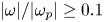 $|{\omega}|/|{\omega _{p}}|\ge 0.1$ (here
 ${\omega _{p}}$ denotes the local vorticity peak) to eliminate noise from the PIV data (Feng & Wang Reference Feng and Wang2010; Xu et al. Reference Xu, Wang, Feng, He and Wang2018). Based on sensitivity analysis, by selecting normalized vorticity levels of 0.05 to 0.2 with 0.05 increment, the circulation of the vortex ring is insensitive to this cut-off level with the difference less than 3 %.
2.4.2. Finite-time Lyapunov exponent
The  ${\lambda _{ci}}$ criterion can effectively identify large-scale vortical structures. However, as vortices break into small scales in the downstream propagation, the results with a smaller threshold of
 ${\lambda _{ci}}$ could be contaminated by noise in the data, leading to a hard observation. The identification of Lagrangian coherent structures (LCSs) provides a robust method to deal with this issue, which can be achieved through computing the finite-time Lyapunov exponent (FTLE) field (Haller & Yuan Reference Haller and Yuan2000; Shadden, Dabiri & Marsden Reference Shadden, Dabiri and Marsden2006).
For a time-dependent flow map  $\boldsymbol{\phi} _{{t_0}}^{{t_0} + {T_F}}({\boldsymbol{x}_0})\,:\boldsymbol{x}({t_0}) \mapsto \boldsymbol{x}({t_0} + {T_F})$ that maps fluid particles from their initial position (
 $\boldsymbol{x}_{0}$, t 0) to their later position over a finite time TF, the Cauchy–Green strain tensor is expressed as (Haller Reference Haller2015)
 \begin{equation}\boldsymbol{C}_{{t_0}}^{{t_0} + {T_F}}({\boldsymbol{x}_0}) = {[\boldsymbol{\nabla }\boldsymbol{\phi} _{{t_0}}^{{t_0} + {T_F}}({\boldsymbol{x}_0})]^\textrm{T}}\boldsymbol{\nabla }\boldsymbol{\phi} _{{t_0}}^{{t_0} + {T_F}}({\boldsymbol{x}_0}),\end{equation}
and the FTLE can be computed as (Green, Rowley & Haller Reference Green, Rowley and Haller2007; Xu et al. Reference Xu, Wang, Feng, He and Wang2018)
 \begin{equation}\textrm{FTL}{\textrm{E}_{{T_F}}}({\boldsymbol{x}_0},{t_0}) = \ln \sqrt {{\lambda _{\textit{max} }}(\boldsymbol{C}_{{t_0}}^{{t_0} + {T_F}}({\boldsymbol{x}_0}))} /|{T_F}|,\end{equation}
where  ${\lambda _{\textit{max} }}(\boldsymbol{C}_{{t_0}}^{{t_0} + {T_F}}({\boldsymbol{x}_0}))$ represents the largest singular value of
 $\boldsymbol{C}_{{t_0}}^{{t_0} + {T_F}}({\boldsymbol{x}_0})$. The LCSs are indicated by ridges in the FTLE field corresponding to the regions of maximum fluid particle separation (
 ${T_F} \gt 0$) or attraction (
 ${T_F} \lt 0$). The ridge in the forward-time (
 ${T_F} \gt 0$) FTLE field represents a repelling LCS, and that in the backward-time (
 ${T_F} \lt 0$) FTLE field represents an attracting LCS. In this study, the 3-D FTLE is computed on a Cartesian grid with a resolution of 0.2 mm × 0.2 mm × 0.2 mm (0.025De × 0.025De × 0.025De) over a backward-time integration of
 ${T_F} ={-} 1.5\;\textrm{s}$, equal to three times the jet cycle (T = 0.5 s). This integration time enables one to identify details of the flow structures in the far-downstream field considering acceptable computational expense. The numerical integration adopts a fourth-order Runge–Kutta method with a time step of 0.01 s, and the space grid is interpolated by trilinear interpolation.
2.4.3. Fourier mode decomposition
Fourier mode decomposition (FMD) is a useful tool to extract important dynamical information from the complex flow (Ma et al. Reference Ma, Feng, Pan, Gao and Wang2015; Qu et al. Reference Qu, Wang, Sun, Feng, Pan, Gao and He2017). The FMD can decompose the flow field into a train of modes corresponding to the coherent structures with a specific frequency based on discrete Fourier transformation (DFT) of the data at each sampling point. When dealing with a quasi-periodic flow, the FMD has similarity in the global power spectrum, and the spatial modes corresponding to the characteristic frequencies with the dynamic mode decomposition method. However, the FMD has fewer limitations in the original data dimension and consumes less calculation time, and thus could be appropriate for the 3-D flow-field decomposition. One can refer to the work of Ma et al. (Reference Ma, Feng, Pan, Gao and Wang2015) for more details of the FMD algorithm. In this study, FMD is used to extract dynamical information from the boundary-layer flow to reveal the impact of the jet.
3. Rectangular synthetic jet in quiescent environment
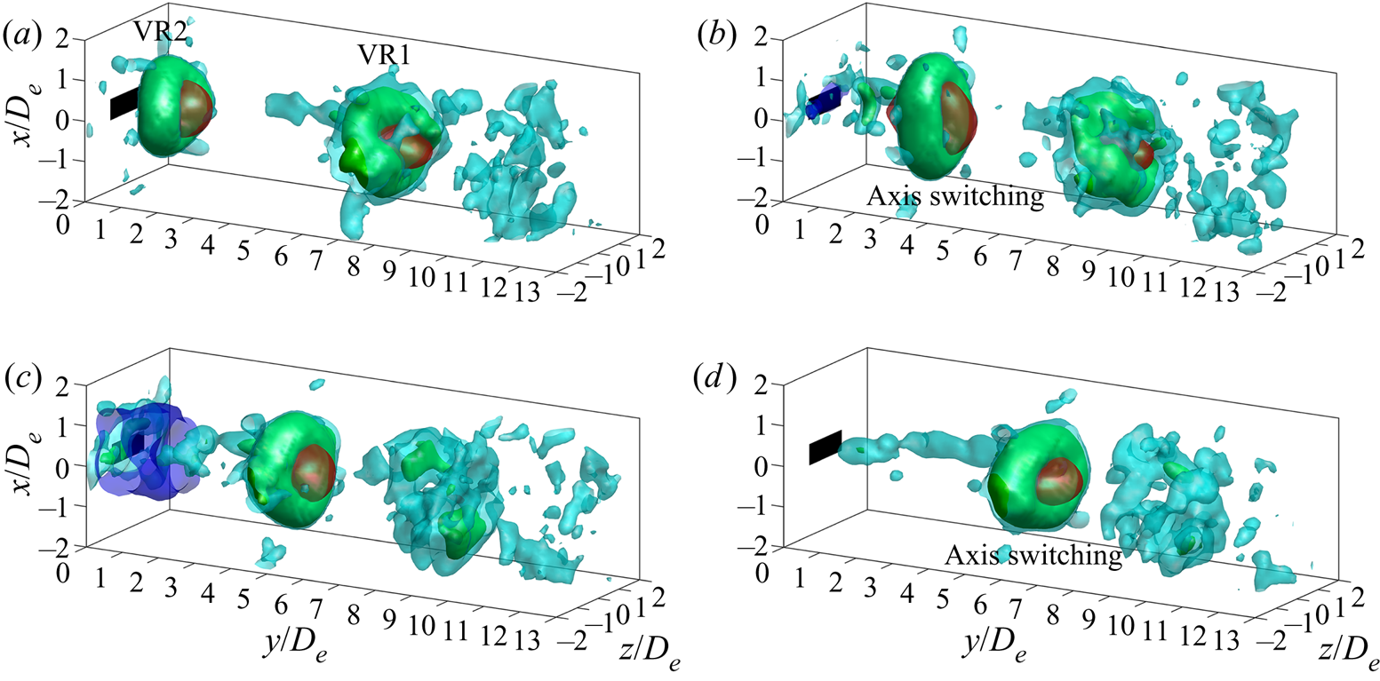
This section focuses on the characteristics of an AR = 3 rectangular synthetic jet issued into a quiescent environment, which can provide the basis for understanding the complex interactions with the cross-flow. Figure 3 shows the temporal evolution of the phase-averaged field for the AR = 3 rectangular synthetic jet. Vortical structures are visualized by isosurfaces of  ${\lambda _{ci}}$, and those corresponding to two typical thresholds of
 ${\lambda _{ci}} = 1.5$ (cyan) and 3.5 (green) are displayed together, which could help to distinguish the flow structures with different scales and strengths.
Temporal evolution of the AR = 3 rectangular free synthetic jet at t/T = 0.25 (a), 0.5 (b), 0.75 (c) and 1 (d). Isosurfaces of phase-averaged  ${\lambda _{ci}} = 1.5$ (cyan) and 3.5 (green), and jet velocity
 ${u_y}/{U_\infty } = 1$ (red) and −0.1 (blue, near the jet exit during the suction period) are presented. VR denotes vortex ring, and 1 and 2 denote the vortical structures from two consecutive cycles.
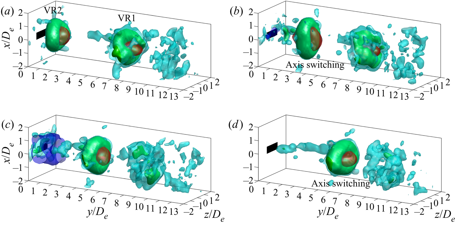
Synthetic jet vortex rings (VR1 and VR2) from two consecutive cycles are observed in the investigated field. Owing to azimuthal non-uniformity of the shear-layer growth rate (Gutmark & Grinstein Reference Gutmark and Grinstein1999), the VR2 immediately initiates self-induced deformation from the jet exit. Such self-induced deformation results in subsequent interchange of the major axis and minor axis of the vortex ring relative to the initial orientations, indicating the first axis switching. With axis switching, the jet velocity with the VR2 exhibits compression and stretching in the initial major-axis and minor-axis directions, respectively (see  ${u_y}/{U_\infty } = 1$ in figure 3b).
It is noticed that, at the maximum suction moment, the synthetic jet produces evident reverse flow at the jet exit (see  ${u_y}/{U_\infty } ={-} 0.1$ in figure 3c). That has little effect on the VR2, which has moved far away from the jet exit. Then the VR2 undergoes the second axis switching, and interchanges its major axis and minor axis again. The jet velocity exhibits opposite variation to that during the first axis switching (figure 3d). After that, the vortex ring becomes more distorted through developing azimuthal instability (Nichols, Schmid & Riley Reference Nichols, Schmid and Riley2007), and eventually breaks into small scales, as reflected by the evolution of the VR1.
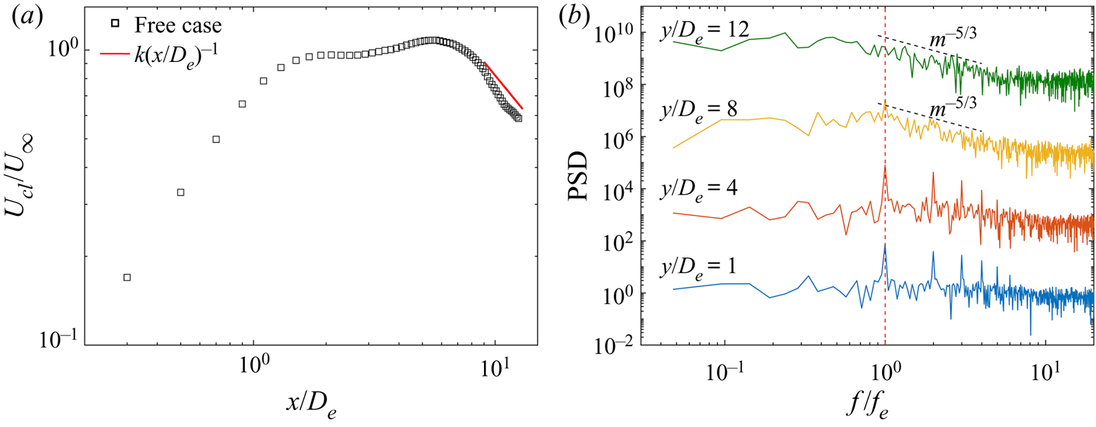
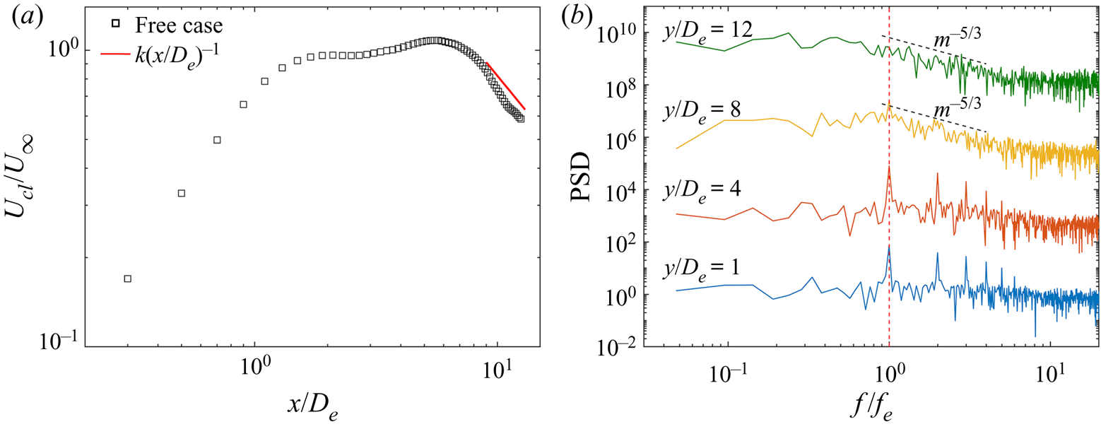
Figure 4 presents the streamwise variation of the time-averaged jet centreline velocity and the related power spectrum to reflect the flow-field characteristics. After reaching the maximum, the downstream behaviour (x/De > 9) of the jet centreline velocity asymptotically approaches an (x/De)−1 decay law, suggesting the tendency of the rectangular synthetic jet towards an axisymmetric turbulent jet. In the power spectra, profound peaks corresponding to the excitation frequency and its high harmonics are observed at y/De = 1 and 4 since the near flow field (x/De < 6) of the synthetic jet is dominated by periodic motion of vortex rings. As the vortical structures break down, the peak of the dominant frequency is gradually reduced, and has disappeared at y/De = 12. Concurrently, the local slope is close to the Kolmogorov scaling of −5/3, reflecting the flow transition to a turbulent one.
(a) Streamwise variation of jet centreline velocity  ${U_{cl}}/{U_\infty }$. (b) Power spectral density (PSD) of jet centreline velocity at y/De = 1, 4, 8 and 12. Each power spectrum has been shifted upward by 103 relative to the former one.
4. Vortical evolution in cross-flow
4.1. Identification of vortical structures
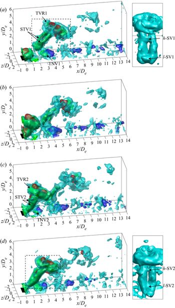
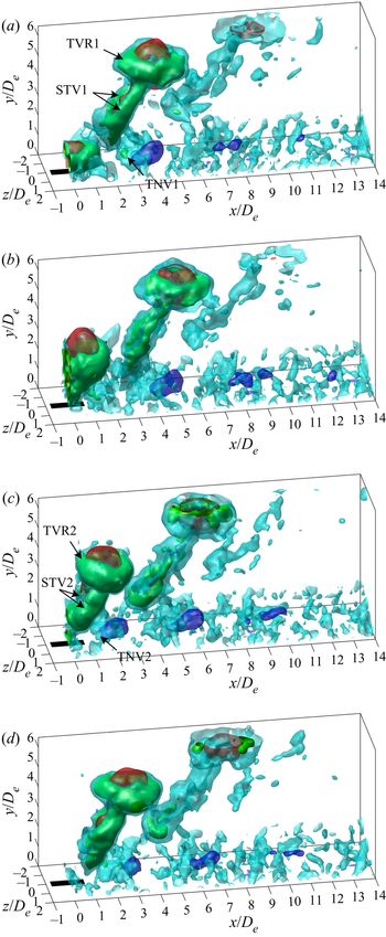
Figures 5 and 6 present the temporal evolution of the phase-averaged fields for the spanwise and streamwise cases, respectively. The vortical structures are visualized by isosurfaces of  ${\lambda _{ci}}$ like those in the quiescent condition. In addition, the vertical velocity
 ${u_y}/{U_\infty } = 0.4$ (red) and −0.04 (blue) is also shown to reflect the local induced velocities of different vortical structures. Owing to the similar components of the vortical structures for the two cases, we give a representative description mainly based on the spanwise case.
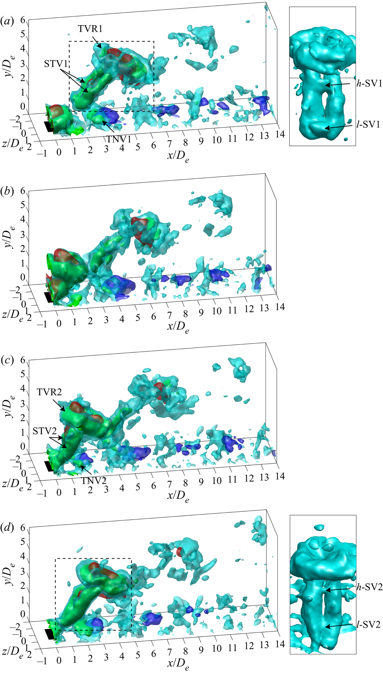
Temporal evolution of the spanwise case at t/T = 0.25 (a), 0.5 (b), 0.75 (c) and 1 (d). Isosurfaces of phase-averaged λci = 1.5 (cyan) and 3.5 (green), and vertical velocity  ${u_y}/{U_\infty } = 0.4$ (red) and −0.04 (blue, in the downstream near-wall region) are presented. Front views zooming-in on the black dashed box are shown on the right of (a) and (d). TVR, STV and TNV denote tilted vortex ring, secondary trailing vortex and tertiary near-wall vortex; h-SV and l-SV denote higher and lower shear-layer vortices, respectively.
Temporal evolution of the streamwise case at t/T = 0.25 (a), 0.5 (b), 0.75 (c) and 1 (d). Identical isosurfaces with those in figure 5 are presented.

As shown in figure 5, the vortical structures for rectangular synthetic jets in cross-flow are composed of a tilted vortex ring (TVR) followed by a secondary trailing vortex (STV). The TVR exhibits downstream tilting, associated with the trailing structures, which establish an obstacle to the cross-flow and inhibit the momentum injection into the downstream branch of the vortex ring. In contrast, the upstream branch has higher momentum, and thus a larger propagation velocity than the downstream one. Consequently, the jet column as well as the vortex ring becomes bent downstream in the cross-flow direction, consistent with the results for pulse jets (Sau & Mahesh Reference Sau and Mahesh2008) and plasma synthetic jets (Zong & Kotsonis Reference Zong and Kotsonis2019) in cross-flow.
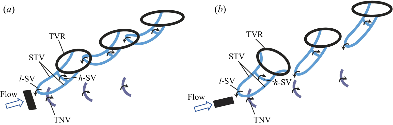
The STV is essentially a pair of counter-rotating vortices branching from the middle of the vortex ring. It has the same rotation sense as the corresponding longitudinal edge of the vortex ring. As a result, an upwash velocity is induced between the two legs of the STV, and inside the vortex ring (see 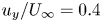 ${u_y}/{U_\infty } = 0.4$). This upwash velocity can lift the low-momentum fluid away from the wall, leading to the local velocity deficit in the lee side of the jet. It is interesting to find that the STV does not extend to the wall, whereas the ends of the two legs are jointed in the spanwise direction by a shear-layer vortex named l-SV. Over the l-SV, another shear-layer vortex is detected to be seated on the STV underneath the upstream branch of the TVR, namely h-SV (see the zoom-in in figure 5a,d). These two shear-layer vortices will be further depicted in figure 7. In addition, a tertiary near-wall vortex (TNV) in a crescent shape is formed near the wall due to induction of the STV and l-SV. The TNV convects with a downwash velocity induced on its downstream side (see
 ${u_y}/{U_\infty } ={-} 0.04$). This downwash velocity can be advantageous for momentum injection near the wall.
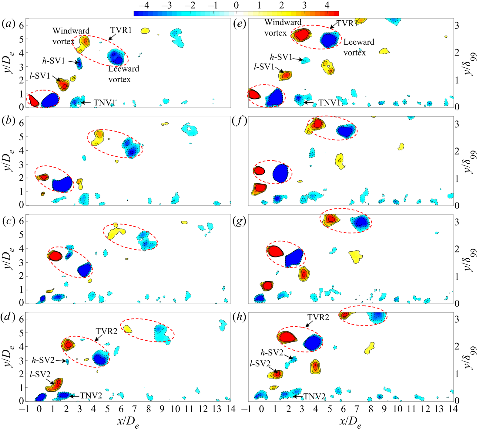
Contours of  ${\lambda _{ci}}{\omega _z}/|{\omega _z}|\textrm{ }({\lambda _{ci}} \ge 1.5)$ in the jet symmetry plane for the (a–d) spanwise and (e–h) streamwise cases at t/T = 0.25 (a,e), 0.5 (b,f), 0.75 (c,g) and 1 (d,h). The upstream and downstream vortices inside the red dashed ellipse denote the windward and leeward vortices of the TVR. Solid and dashed lines represent positive and negative values, respectively. Contour levels are ±1.

The current flow scenarios exhibit vortex rings that convect downstream and penetrate the boundary layer ( ${\delta _{99}} \approx 2{D_e}$). These features have also been observed in the numerical results of Ravi et al. (Reference Ravi, Mittal and Najjar2004) for rectangular synthetic jets with ARs of 1, 2 and 4 in cross-flow. The difference is that their vortices penetrated out of the boundary layer with a longer streamwise distance due to the relatively low VR of 0.5. However, the vortex rings were not formed in previous studies of high-AR (AR > 5) rectangular synthetic jets in cross-flow (Van Buren et al. Reference Van Buren, Beyar, Leong and Amitay2016a,Reference Van Buren, Beyar, Leong and Amitayb). In addition, some differences in the vortical structures can be found in comparison with the tilted and distorted vortex rings for circular synthetic jets (Jabbal & Zhong Reference Jabbal and Zhong2010), which are summarized as follows: the legs of the present STV are connected in the spanwise direction by the two shear-layer vortices at different wall-normal heights, and the present TNV is a crescent-shaped spanwise vortex rather than a longitudinal streamwise vortex pair as in Jabbal & Zhong (Reference Jabbal and Zhong2010).
Contours of  ${\lambda _{ci}}{\omega _z}/|{\omega _z}|\textrm{ }({\lambda _{ci}} \ge 1.5)$ in the jet symmetry plane for the two cases are compared in figure 7. The red dashed ellipse surrounding the windward and leeward vortices of the TVR can reflect the tilting angle. As the vortical structures move away from the wall, the TVR is gradually recovered to the wall-parallel orientation associated with the Biot–Savart induced effect under the cross-flow. As the STV becomes weak and breaks downstream, its inhibition to the cross-flow is diminished. According to the Kutta–Joukowski theorem, the windward vortex of the vortex ring experiences a downward force, while the leeward vortex experiences an upward force, leading to upstream tilting of the vortex ring (Sau & Mahesh Reference Sau and Mahesh2008). In particular, the vortex ring for the streamwise case exhibits faster recovery of the tilting angle and penetration through the boundary layer.
In addition, the shear-layer vortices are detected in the jet symmetry plane for the two cases that have a clockwise rotation for the h-SV, and an anticlockwise rotation for the l-SV. The l-SV is generated by the shear layer rolling-up in the windward side of the initial jet. However, the h-SV evidently differs from the l-SV, and has not been identified in previous research. It is inferred that the h-SV is resulted from the shear between high-momentum, outer cross-flow and low-momentum, near-wall fluid lifted by the STV, akin to the formation mechanism of the secondary and tertiary hairpin vortices in Zhou & Zhong (Reference Zhou and Zhong2010).
4.2. Axis switching in cross-flow
Axis switching of vortex rings is a crucial mechanism for non-circular jets in quiescent condition, by which they can significantly enhance entrainment and mixing relative to comparable circular and 2-D jets (Gutmark & Grinstein Reference Gutmark and Grinstein1999; Grinstein Reference Grinstein2001). However, for steady jets in cross-flow, axis switching no longer happens to non-circular orifices since the presence of a counter-rotating vortex pair inhibits the formation of the vortex ring (Lim, New & Luo Reference Lim, New and Luo2001; New et al. Reference New, Lim and Luo2003). For synthetic jets in cross-flow, vortex rings revert to primary structures as the form of stretched or tilted vortex rings. Hence, whether vortex rings can experience axis switching is of practical interest for non-circular synthetic jets in cross-flow. To our knowledge, no existing research has reported this.
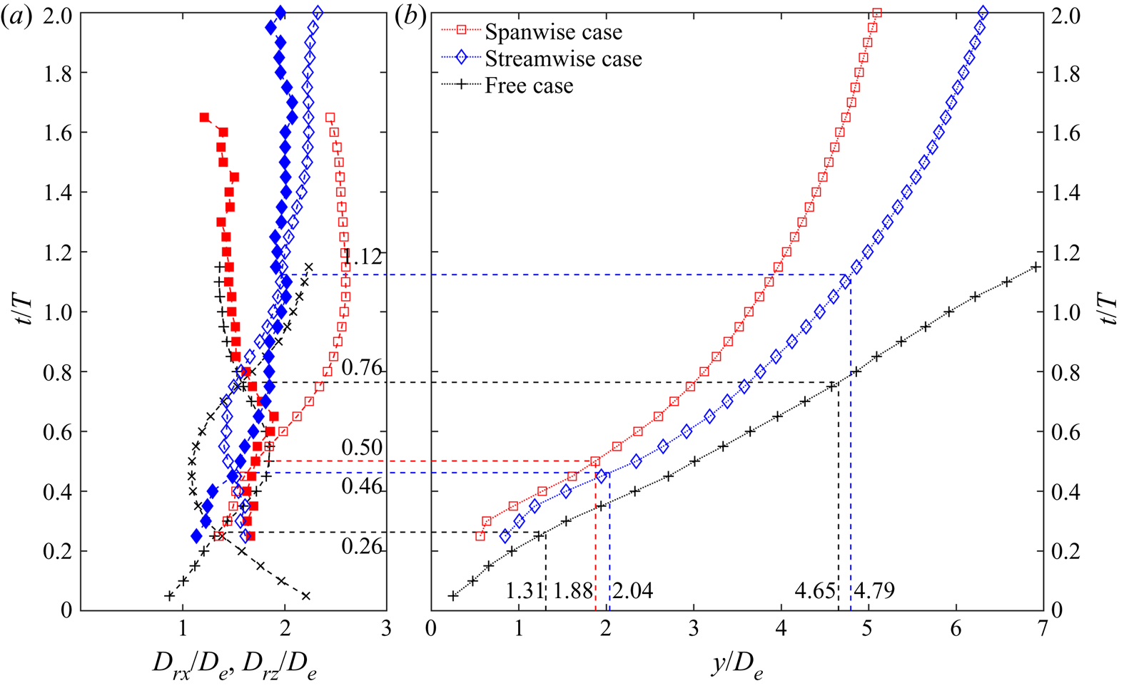
The variation of the vortex ring diameter in the characteristic plane can reflect axis switching of vortex rings, which is defined as the distance between vortex centres corresponding to the positive and negative vorticities. Further, the vortex ring centre is obtained from the middle of the vortex ring diameter in the jet symmetry plane. Figure 8 shows the temporal evolution of the vortex ring diameter and vortex ring centre for the two cases, and the result for the free case is presented for comparison. For the vortex area identified by  ${\lambda _{ci}} = 1.5\;{\textrm{s}^{ - 1}}$, the uncertainty of the vortex ring diameter is approximately 5 %. In addition, the influence of the vortex area on the vortex ring diameter has also been analysed by selecting the
 ${\lambda _{ci}}$ thresholds of 0.5 to 2 s−1 with 0.5 s−1 increment. The variation of the vortex area is found to have little effect on the vortex ring diameter, and the difference of the present result could be within 5 %.
(a) Temporal evolution of vortex ring diameters Drx/De and Drz/De: Drx (—+—) and Drz (—×—) denote the vortex ring diameters in the y–x and y–z planes for the free case; Drx (—□—, spanwise case; —◊—, streamwise case) and Drz (—■—, spanwise case; —♦—, streamwise case) denote the vortex ring diameters in the x–y plane, and the plane through the vortex ring centre and normal to the vortex ring tilting plane. (b) Trajectory of vortex ring centre along the wall-normal direction for the three cases.

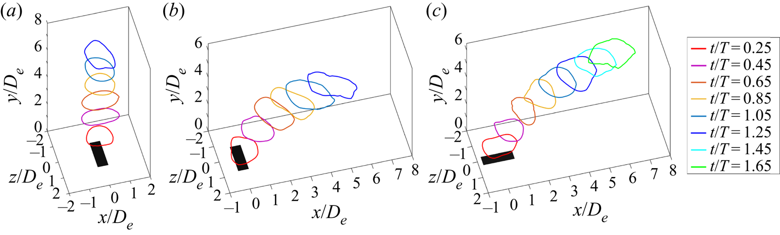
The diameter curves for the free case have two intersection points corresponding to two axis switchings. It is worth noting that the intersection also exists for the spanwise and streamwise cases, respectively, suggesting that the present rectangular synthetic jets in cross-flow can experience axis switching of vortex rings. This is an important difference between non-circular synthetic jets and steady jets in cross-flow. Specifically, the spanwise case undergoes once, while the streamwise case undergoes twice. In addition, the spanwise case has the latest first axis switching (t/T = 0.50), whereas the location (y/De = 1.88) is lower than that of the streamwise case (y/De = 2.04) due to slower vortex penetration (figure 8b).
Axis switching for the three cases can be intuitively displayed by the vortex filament through the vortex centre, as shown in figure 9. For the free case, the cylindrical coordinate system (r, θ, y) is used to determine the vortex centre location (rv, yv) in the radial plane by changing θ by 3° increments. The entire vortex centre locations are connected by a spline curve to obtain the vortex filament. For the case in cross-flow, rotation and translation of the coordinate are performed firstly to keep the vortex ring axisymmetric about the y-axis through the origin. Then the same method as the above is used to obtain the vortex filament, which is finally restored to the original spatial location.
Temporal evolution of vortex filament through vortex centre for the (a) free, (b) spanwise and (c) streamwise cases, respectively.

Compared to self-induced deformation for the free case, the vortex deformation for the spanwise and streamwise cases can be affected by the cross-flow. Owing to the obstacle of the trailing structures to the cross-flow near the wall, the upstream section of the vortex filament is mainly affected by the cross-flow relative to the downstream one. For the spanwise case, the cross-flow has opposite direction to the azimuthal induced velocity of the upstream section, resulting in an unfavourable effect on the local vortex deformation. Conversely, the downstream section yields relatively larger streamwise stretching (see t/T = 0.25 in figure 9b). As the vortex filament moves away from the wall, the impact of the cross-flow on the downstream section increases. As a result, the vortex filament is evidently stretched in the streamwise direction after the first axis switching (see t/T = 1.25 in figure 9b), which can also be reflected by the vortex ring diameter in the jet symmetry plane (figure 8a). Hence, no new axis switching follows.
On the contrary, the initial azimuthal induced velocity of the upstream section has the same direction as the cross-flow for the streamwise case, leading to a favourable effect on the local vortex deformation. Consequently, the streamwise case has an earlier first axis switching than the spanwise case as depicted in figure 8. Additionally, the streamwise case has slower streamwise stretching under the cross-flow, and therefore the vortex filament can experience two axis switchings like the free case.
4.3. Vortex interactions
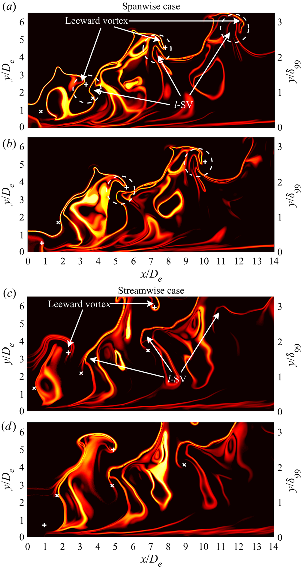
Owing to the periodic property of synthetic jets, interactions between different vortical structures are important for synthetic jets in cross-flow. The FTLE enables one to effectively identify the details of vortical evolution in the far-downstream field. Figure 10 exhibits contours of the backward-time FTLE in the jet symmetry plane for the two cases. The leeward vortex of the TVR is observed to interact with the downstream l-SV for the spanwise case. They approach each other and become a pair of contour-rotating vortices. Then the l-SV is entrained by the leeward vortex into the TVR as the vortical structures propagate downstream, as marked by white dashed circles in figure 10(a,b). However, such a process does not happen to the streamwise case, where the leeward vortex moves away from the l-SV with vortex penetration.
Contours of normalized backward-time FTLE in the jet symmetry plane at t/T = 0.75 (a,c) and 1.25 (b,d) for the (a,b) spanwise and (c,d) streamwise cases. The + and × denote vortex centre locations of the leeward vortex and the l-SV, respectively.

The schematics in figure 11 can aid 3-D illustration of the difference between the two cases. Compared to the independent TVR and STV for the streamwise case, the spanwise case can form a chain of TVRs connected by STVs due to the above vortex interactions, resulting in slower vortex penetration and recovery of the vortex ring tilting. The axis switching properties of the two cases can account for this difference. For the spanwise case, the vortex ring expands its diameter in the jet symmetry plane during the first axis switching (see figure 8a), which reduces the distance between the leeward vortex and the downstream l-SV, and triggers the subsequent vortex interaction. In contrast, the vortex ring for the streamwise case shrinks its diameter in the jet symmetry plane during the first axis switching, and thus impedes the probable interaction.
Schematic models of rectangular synthetic jets in cross-flow with (a) spanwise and (b) streamwise configurations. The black arrows denote the local rotation sense of vortical structures.

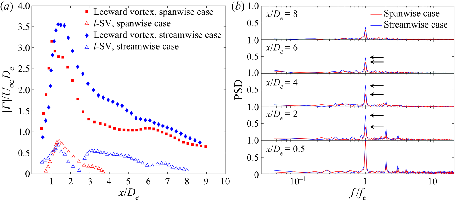
A quantitative description of the vortex interaction effect is presented in figure 12. The formation of a counter-rotating vortex pair can weaken the strengths of the leeward vortex and the l-SV. Thus, the leeward vortex for the spanwise case displays an earlier decay of the circulation to a lower magnitude at around x/De = 3. Furthermore, the circulation of the l-SV cannot be detected after x/De = 4 for the spanwise case, while that is maintained to the downstream field for the streamwise case (figure 12a). Similar behaviour is also observed in the normalized power spectrum of the vertical velocity along the vortex-ring-centre trajectory (figure 12b). The normalization is performed to exhibit the relative variation of the dominant frequency peak more clearly. Compared to the streamwise case, the peaks of the dominant frequency and high-frequency harmonics for the spanwise case decrease more rapidly from x/De = 0.5 to 4 (see the black arrow locations), suggesting faster jet transition under vortex interactions. Note that these flow-field characteristics are essentially the results of axis switching of vortex rings, which can be conducive to enhancing jet mixing and heat transfer for the spanwise case. On the other hand, the trailing structures for the streamwise case have greater streamwise persistency. They in turn can induce larger upwash velocity, leading to a larger velocity deficit in the free stream, which will be demonstrated later.
(a) Circulations of the leeward vortex and the l-SV, and (b) normalized PSD of vertical velocity Uy by the maximum along the vortex-ring-centre trajectory at x/De = 0.5, 2, 4, 6 and 8 for the two cases. The black arrows in (b) mark the peak locations of the dominant frequency.

5. Flow-field characteristics in cross-flow
5.1. Mean flow field in the jet symmetry plane
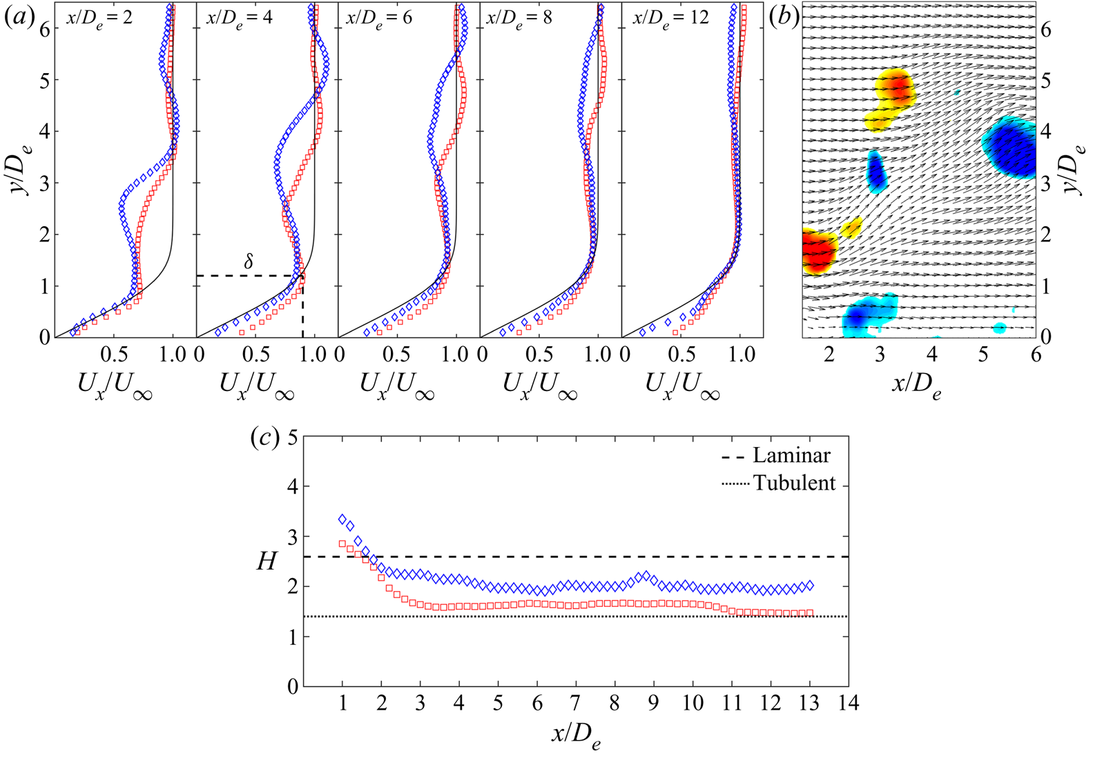
This section pays attention to the flow-field characteristics of rectangular synthetic jets in cross-flow, and discusses the impact of the orifice orientation on the downstream boundary layer. Figure 13(a) presents the time-averaged streamwise velocity profiles at different streamwise locations in the jet symmetry plane. The local contour of  ${\lambda _{ci}}{\omega _z}/|{\omega _z}|$ for the spanwise case is provided in figure 13(b) to help understanding. A prominent velocity deficit can be observed in the near-field profiles, and the magnitude decreases with the jet uplifting. This velocity deficit is attributed to the upwash induced between the legs of the trailing structures, and inside the tilted vortex ring. In particular, the maximum velocity deficit of the spanwise case is lower than that of the streamwise case. That is associated with vortex interactions, which restrict persistency of the trailing structures, and weaken the vortex strength, as depicted in figure 12. However, this comparison is opposite to the previous results for steady jets (Gutmark, Ibrahim & Murugappan Reference Gutmark, Ibrahim and Murugappan2008) and higher-AR synthetic jets (Van Buren et al. Reference Van Buren, Beyar, Leong and Amitay2016b) in cross-flow. The difference can be accounted for by no axis switching and following vortex interactions observed in those studies.
(a) Time-averaged streamwise velocity profile  ${U_x}/{U_\infty }$, (b) local contour of
 ${\lambda _{ci}}{\omega _z}/|{\omega _z}|$ (
 ${\lambda _{ci}} \ge 1.5$, t/T = 0.25 for the spanwise case) superposed by velocity vector, and (c)boundary-layer shape factor H in the jet symmetry plane, for □ (red), the spanwise case, and ◊ (blue), the streamwise case. The black solid line in (a) represents the Blasius profile, and the black dashed line at x/De = 4 denotes the definition for the boundary-layer thickness δ.

In addition, velocity overshoot appears on both sides of the velocity deficit region. The upper velocity overshoot results from local induced velocity upon the leeward vortex, while that inside the boundary layer after x/De = 4 is due to momentum transfer by the near-wall vortex. With the merging between the jet and the boundary layer, the velocity in the boundary-layer profile does not recover to the free-stream value. Hence, the current boundary-layer thickness cannot be determined by the traditional 99 %  ${U_\infty }$ criterion. According to the definition suggested by Sarkar & Sarkar (Reference Sarkar and Sarkar2009), we use the height of the local maximum of Ux between the wall and the velocity deficit region as the local boundary-layer thickness
 $\delta $, as shown by the black dashed line at x/De = 4. Thus, the boundary-layer shape factor can be calculated as
 \begin{equation}H = \frac{{\int_0^\delta {\left( {1 - \frac{{{U_x}}}{{{U_{x,\textit{max} }}}}} \right)\,\textrm{d}y} }}{{\int_0^\delta {\frac{{{U_x}}}{{{U_{x,\textit{max} }}}}\left( {1 - \frac{{{U_x}}}{{{U_{x,\textit{max} }}}}} \right)\,\textrm{d}y} }},\end{equation}
where  ${U_{x,\textit{max} }}$ denotes the local maximum of Ux. The result in figure 13(c) indicates that the shape factor of the spanwise case is closer to the turbulent value (H = 1.4), corresponding to the larger velocity gradient inside the boundary layer.
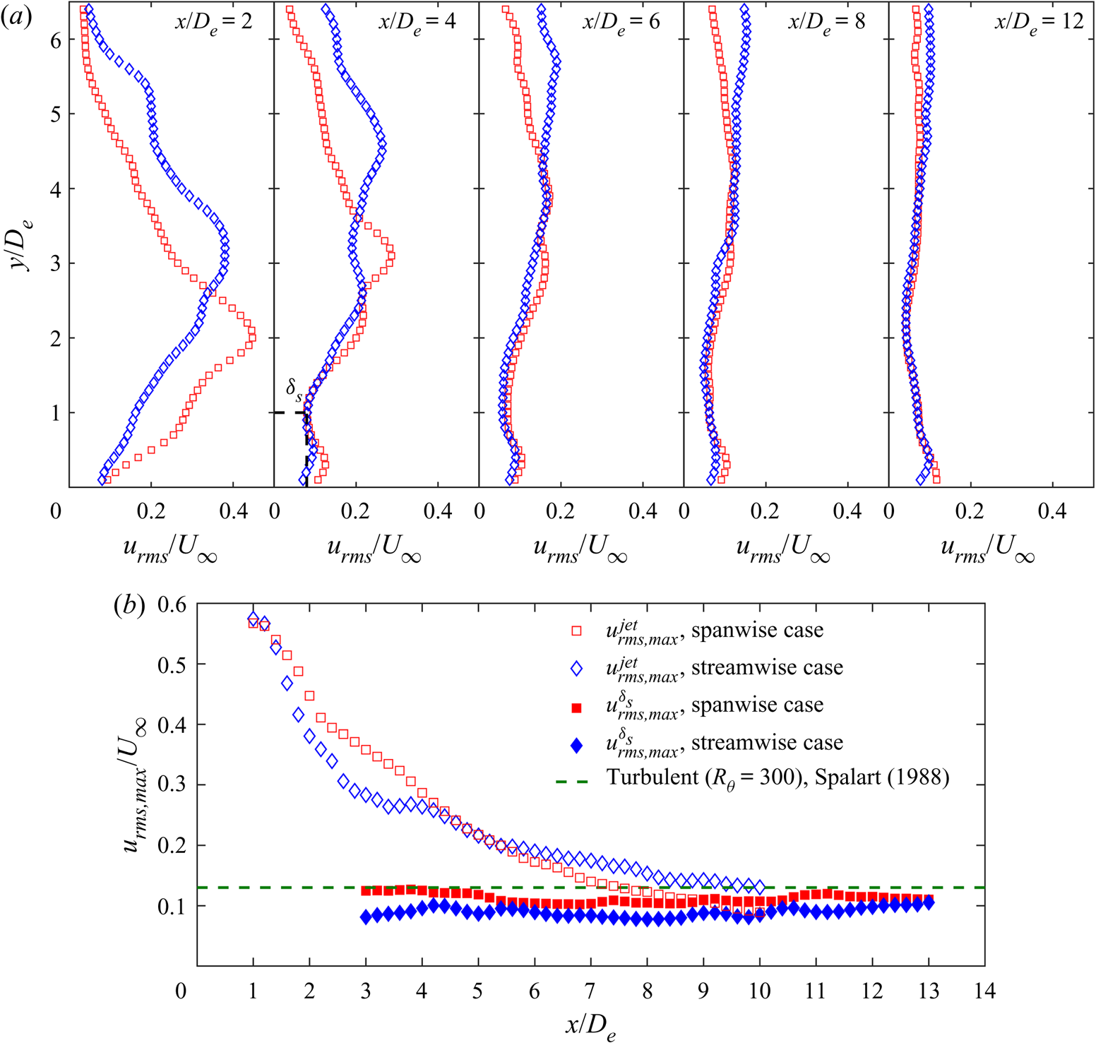
The streamwise velocity fluctuation profiles in the jet symmetry plane are displayed in figure 14(a). The local peaks of velocity fluctuation in the jet region are caused by the tilted vortex ring and the shear-layer vortices. The corresponding maximum velocity fluctuation  $u_{rms,\textit{max} }^{jet}$ decreases with the jet uplifting (figure 14b). Since the spanwise case is more bent downstream by the cross-flow, it can produce slightly larger
 $u_{rms,\textit{max} }^{\,jet}$ than the streamwise case before x/De = 4. However, as the trailing structures break down under vortex interactions, the spanwise case has a larger decay rate after x/De = 5.
(a) Streamwise velocity fluctuation profile  ${u_{rms}}/{U_\infty }$, and (b) maximum velocity fluctuation in the jet region
 $u_{rms,\textit{max} }^{jet}$, and the sheltering edge
 $u_{rms,\textit{max} }^{{\delta _s}}$ in the jet symmetry plane, for □ (red), the spanwise case, and ◊ (blue), the streamwise case. The black dashed line at x/De = 4 in (a) denotes the definition for the sheltering edge δs.

A new peak can be observed inside the boundary layer at around y/De = 0.3 (spanwise case) or 0.4 (streamwise case) downstream of x/De = 4 (figure 14a), which is contributed by the near-wall vortex. Following He, Wang & Pan (Reference He, Wang and Pan2013), an inflection point at the minimum of urms between the near-wall peak and the outside peak can be determined to define a sheltering edge  ${\delta _s}$, as shown by the black dashed line at x/De = 4. The sheltering edge is slightly smaller than
 $\delta $, which can be used to exclude the jet's direct disturbance from the boundary layer in the later analysis. The spanwise case has a larger maximum velocity fluctuation inside the sheltering edge
 $u_{rms,\textit{max} }^{{\delta _s}}$ than the streamwise case (figure 14b), close to the value of a canonical turbulent boundary layer (Spalart Reference Spalart1988). This result is perceived to stem from the larger upstream jet disturbance which is transferred into the boundary layer through the near-wall vortex.
5.2. Mean flow field in the spanwise plane
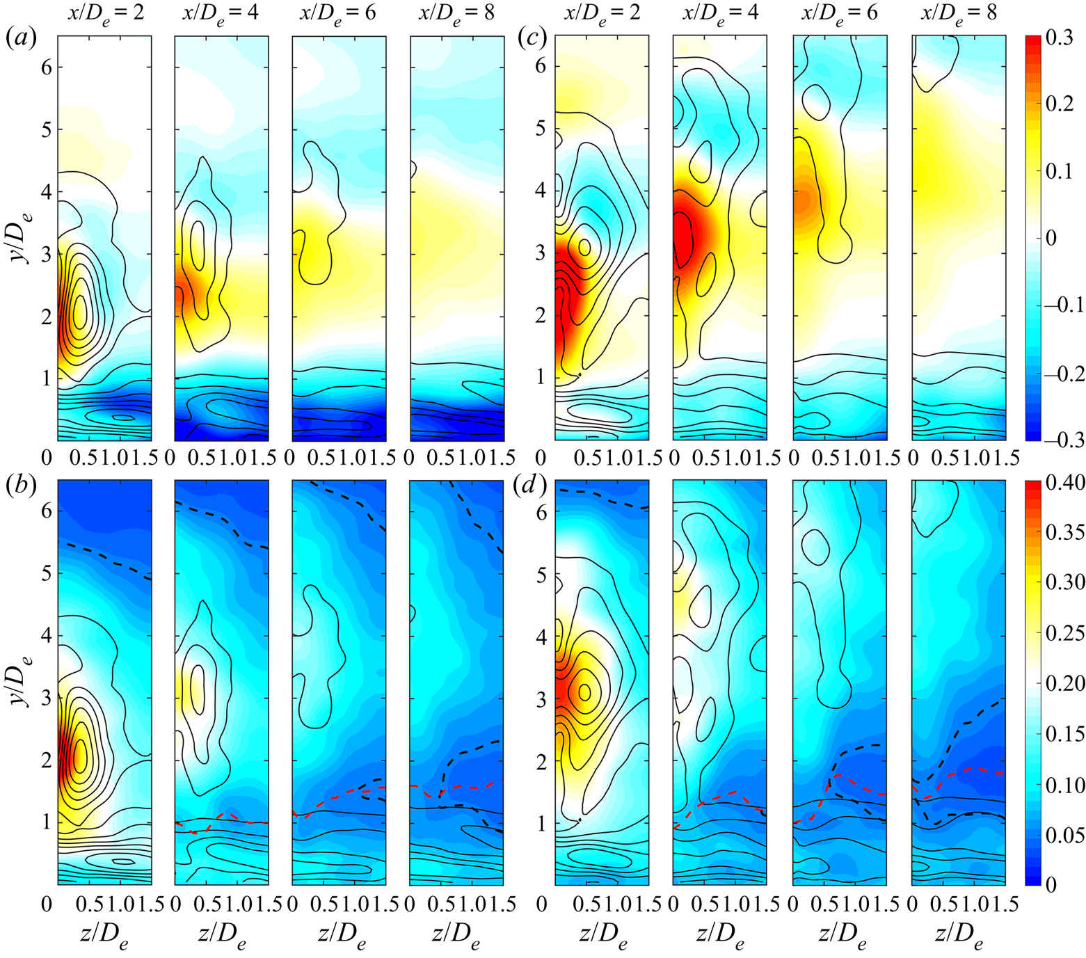
Figure 15(a,c) presents the spanwise distribution of the velocity deficit and overshoot  $({{U_{BL}} - {U_x}} )/{U_\infty }$ (here UBL denotes the Blasius profile), superposed by the local time-averaged vorticity
 $|{\bar{\omega }_{xyz}}|{D_e}/{U_\infty }\textrm{ }(|{\bar{\omega }_{xyz}}|= \sqrt {\bar{\omega }_x^2\; + \; \bar{\omega }_y^2\; + \; \bar{\omega }_z^2} )$. A positive value of
 $({{U_{BL}} - {U_x}} )/{U_\infty }$ represents a velocity deficit and a negative value represents a velocity overshoot. Associated with weaker trailing structures and vortex ring (see
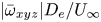 $|{\bar{\omega}_{xyz}}|{D_e}/{U_\infty }$ in the jet region), the spanwise case exhibits lower peaks of the velocity deficit and overshoot than the streamwise case in the jet region. In contrast, the peak of the velocity overshoot inside the boundary layer is larger for the spanwise case.
Spanwise distributions of (a,c) velocity deficit and overshoot  $({U_{BL}} - {U_x})/{U_\infty }$, and (b,d) streamwise velocity fluctuation
 ${u_{rms}}/{U_\infty }$ for the (a,b) spanwise and (c,d) streamwise cases. The black solid line denotes the time-averaged vorticity
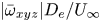 $|{\bar{\omega }_{xyz}}|{D_e}/{U_\infty }$ with minimum value of 0.2 and interval of 0.2; the black dashed line in (b,d) denotes the contour of
 ${u_{rms}}/{U_\infty } = 0.05$; and the red dashed line denotes the sheltering edge δs.

The spanwise distribution of the streamwise velocity fluctuation is shown in figure 15(b,d). Owing to slower vortex penetration, the impact of the jet disturbance on the boundary layer can persist more downstream for the spanwise case. For instance, the disturbance of  ${u_{rms}}/{U_\infty } = 0.05$ is jointed between the jet and the boundary layer at x/De = 8 for the spanwise case; however, that has been completely separated by the local sheltering edge for the streamwise case. Accordingly, the spanwise case has larger velocity fluctuation peak inside the boundary layer, displaying the merit of promoting boundary-layer transition.
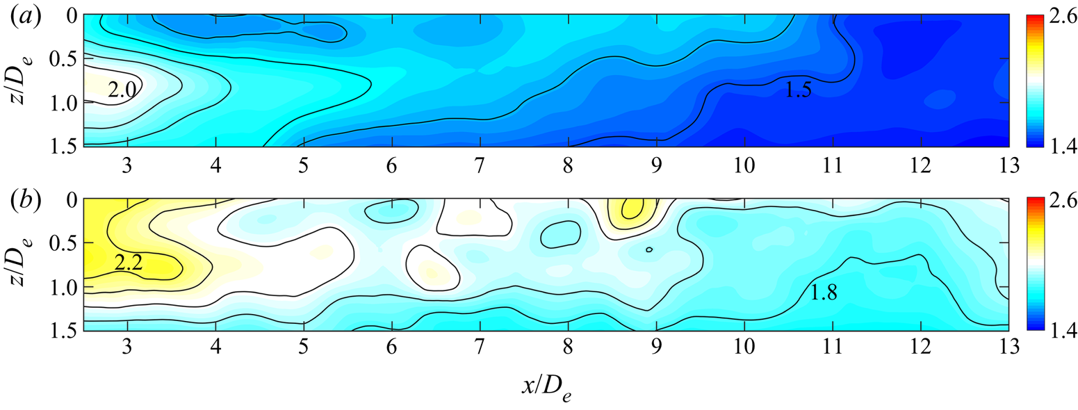
Using (5.1), the spatial distribution of the boundary-layer shape factor is given in figure 16. Overall, the boundary-layer shape factors for the two cases decrease in the streamwise direction, reflecting the trend of boundary-layer transition to a turbulent one. Inparticular, the global shape factor of the spanwise case is lower than that of the streamwise case, consistent with the characteristics of larger velocity gradient and velocity fluctuation peak inside the boundary layer. This suggests that the spanwise orifice orientation could be more efficient to energize the boundary layer for resisting streamwise adverse pressure gradients.
Spatial distribution of boundary-layer shape factor H for the (a) spanwise and (b) streamwise cases. Contour levels are 0.1.

5.3. Disturbance development inside boundary layer
Based on the above analysis, the boundary-layer transition in the lee side of the jet is associated with the near-wall vortex induced by synthetic jets. To further reveal the disturbance impact of the near-wall vortex on the boundary layer, the FMD method is used to extract the relevant dynamical information. The flow field in the range of [1, 14]De × [0, 4]De × [−1.5, 1.5]De in three directions is selected to perform the FMD, which contains the entire boundary-layer region downstream of the jet.
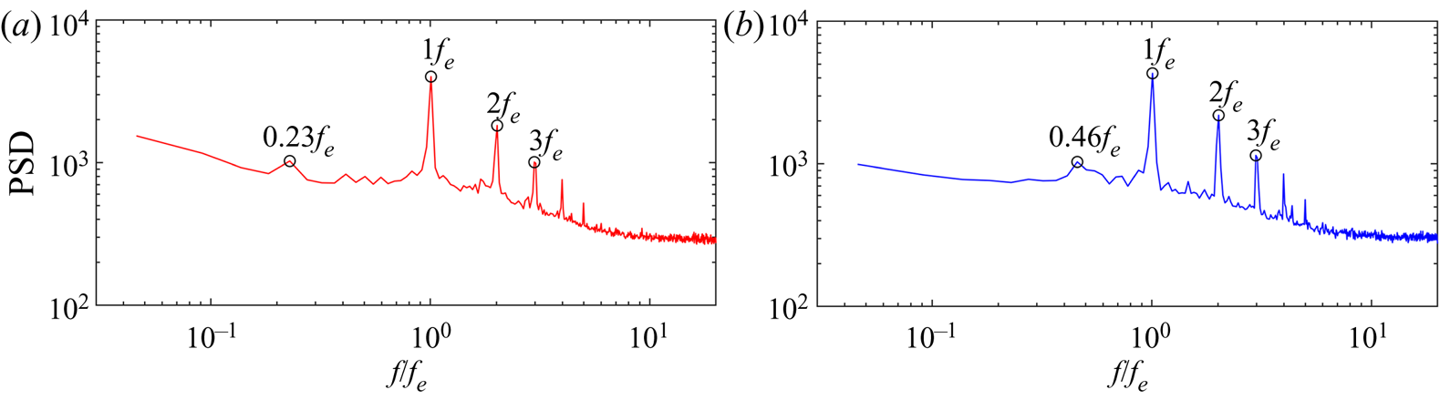
Figure 17 presents the global FMD power spectrum of the selected flow field for the three velocity components at each sampling point. The power spectra of the two cases both display profound peaks corresponding to the excitation frequency and its high-frequency harmonics. In addition, the peaks at lower frequencies of 0.23fe for the spanwise case, and 0.46fe for the streamwise case, can be detected corresponding to the low-frequency disturbance components.
Global FMD spectrum of the selected region for the (a) spanwise and (b)streamwise cases.

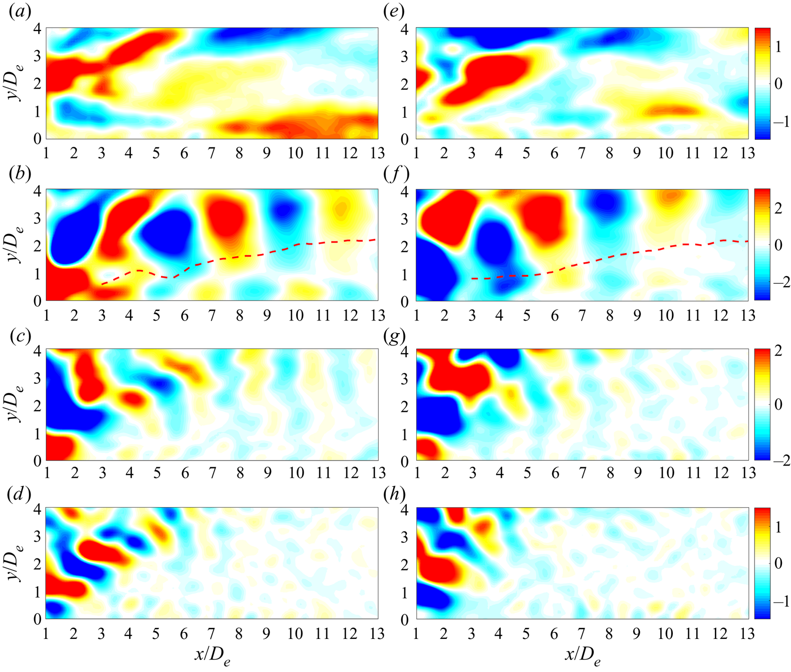
The spatial FMD modes with the marked characteristic frequencies are examined, and figure 18 shows the streamwise components of these modes in the jet symmetry plane. Only the imaginary part of each spatial mode is given due to the conjugate relation between the real and imaginary parts. The modes upon the boundary layer reveal the jet structures with different spatial scales. The streamwise wavelength of these structures decreases with increased frequency. Inside the boundary layer, the near-wall modes with the dominant frequency of 1.0fe characterize the downstream convection of the near-wall vortex (figure 18b,f).
Streamwise components of FMD modes in the jet symmetry plane with different frequencies for the two cases: (a) 0.23fe, (b) 1.0fe, (c) 2.0fe and (d) 3.0fe for the spanwise case; (e) 0.46fe, (f) 1.0fe, (g) 2.0fe and (h) 3.0fe for the streamwise case. The red dashed line in (b,f) denotes the sheltering edge.

At a lower frequency of 0.23fe, it is noted that an elongated structure with considerably large spatial scale appears at the downstream location for the spanwise case (figure 18a), similar to the result of boundary-layer transition induced by a circular cylinder wake in He et al. (Reference He, Wang and Pan2013). This suggests that the low-frequency disturbance of 0.23fe can persist downstream independent of the external excitation frequency. In fact, similar structures with different spatial scales can also be found in some other low-frequency modes. For the streamwise case, the elongated structures are weaker (figure 18e), probably due to the relatively lower disturbance amplitude, which will be presented in figure 19. At higher frequencies of 2.0fe and 3.0fe, no near-wall modes with comparable amplitude relative to those in the jet region are observed.
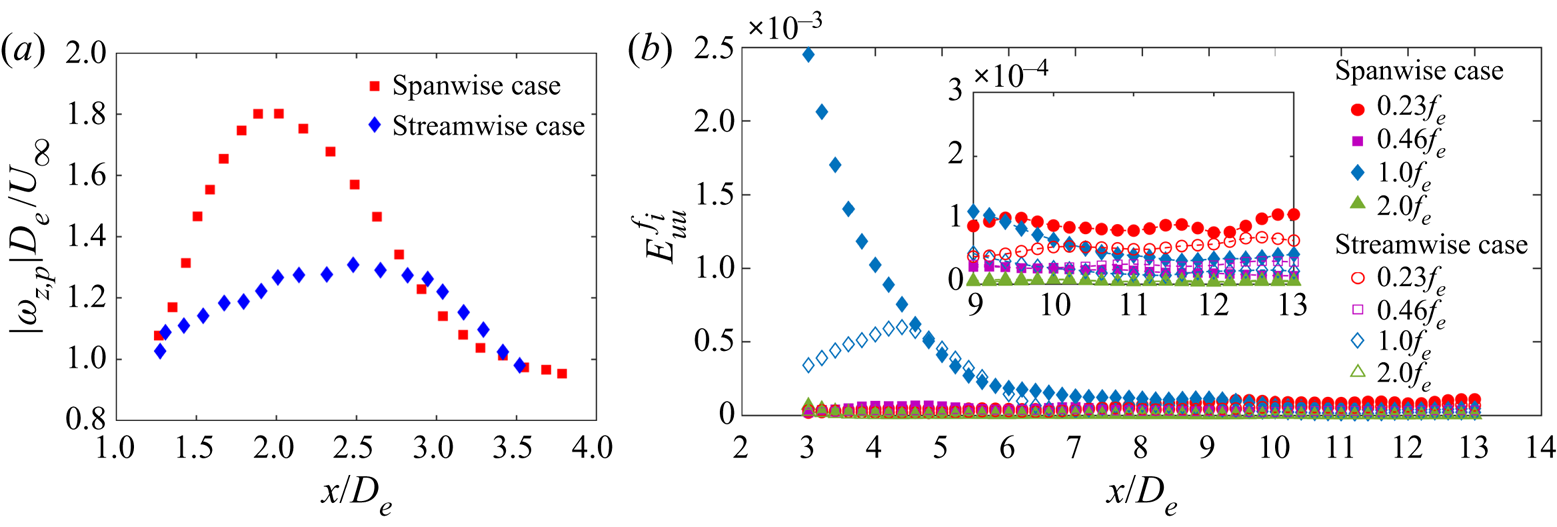
Streamwise evolution of (a) vorticity peak  $|{\omega _{z,p}}|{D_e}/{U_\infty }$ of the near-wall vortex, and (b) averaged boundary-layer disturbance energy
 $E_{uu}^{{f_i}}$ of the FMD modes with different frequencies fi for the two cases.

To quantitatively measure the disturbance amplitude of different frequencies, we compute the averaged boundary-layer disturbance energy  $E_{uu}^{{f_i}}$ with a frequency fi as
 \begin{equation}E_{uu}^{{f_i}} = {{\int {\int_0^{{\delta _s}} {(u_{rms}^{{\,f_i}})^2\,\textrm{d}y\,\textrm{d}z} } } \bigg / {\int {\int_0^{{\delta _s}} {U_\infty ^2\,\textrm{d}y\,\textrm{d}z} ,} }}\end{equation}
where  $u_{rms}^{{f_i}}$ represents the streamwise velocity fluctuation of the flow field with the frequency fi. Note that the integral upper limit here is selected as
 ${\delta _s}$ instead of
 $\delta $ to exclude the direct contribution of the jet disturbance. The boundary-layer disturbance energies of the selected frequencies (0.23fe, 0.46fe, 1.0fe and 2.0fe) for the two cases are compared in figure 19(b), and the vorticity peak of the near-wall vortex is given in figure 19(a) to aid interpretation.
As shown in figure 19(b), compared to the streamwise case, the disturbance energy of 1.0fe for the spanwise case has significantly larger initial magnitude followed by a faster decay in the near flow field (x/De < 6). This result is ascribed to the stronger near-wall vortex for the spanwise case (figure 19a), which yields larger initial disturbance to trigger boundary-layer transition. Additionally, the short growth stage of 1.0fe for the streamwise case could be related to the more downstream vorticity peak of the near-wall vortex. Since the current boundary-layer flow is in the early stage of the transition, the disturbance energies of the low-frequency components grow at a much slow rate. Even so, the magnitude of 1.0fe has decayed to be lower than that of 0.23fe after approximately x/De = 9.3 for the two cases. Particularly, 0.23fe for the spanwise case has the largest disturbance magnitude corresponding to more turbulent characteristics. Such a result can help to understand the mechanism of boundary-layer transition induced by synthetic jets.
6. Conclusions
In this paper, we experimentally investigate the 3-D flow fields of an AR = 3 rectangular synthetic jet and its interaction with a laminar cross-flow using time-resolved tomographic PIV. Two typical orifice orientations, spanwise and streamwise configurations, are concerned to analyse the vortical evolution and the relevant flow physics.
Compared to the quiescent condition, the vortical structures for rectangular synthetic jets in cross-flow are more complicated, which are composed of a tilted vortex ring (TVR), a secondary trailing vortex (STV) and a tertiary near-wall vortex (TNV). The flow scenarios are evidently different from those for high-AR (AR > 5) cases (Van Buren et al. Reference Van Buren, Beyar, Leong and Amitay2016a,Reference Van Buren, Beyar, Leong and Amitayb). Also, some differences are found compared with the tilted and distorted vortex rings for circular cases (Jabbal & Zhong Reference Jabbal and Zhong2010): the legs of the present STV are jointed in the spanwise direction by two shear-layer vortices at different wall-normal heights, named l-SV and h-SV; the present TNV is a crescent-shaped spanwise vortex instead of a streamwise vortex pair as in Jabbal & Zhong (Reference Jabbal and Zhong2010).
For the first time, as the peculiar property of non-circular vortex rings in quiescent condition, axis switching is detected for low-AR rectangular synthetic jets in cross-flow. The orifice orientation has a direct impact on the time and location of axis switching. Furthermore, axis switching can cause vortex interaction for the spanwise case, where the leeward vortex of the TVR and the downstream l-SV become a pair of contour-rotating vortices. As a result, the spanwise case forms a chain of TVRs connected by the STVs; however, they are relatively independent for the streamwise case. Under vortex interactions, the spanwise case yields slower recovery of the vortex ring tilting and penetration through the boundary layer, but faster jet transition.
The time-averaged flow fields in the jet symmetry and spanwise planes are examined, respectively. Owing to weaker trailing structures and vortex ring, the spanwise case exhibits lower peaks of the velocity deficit and overshoot in the jet region. In contrast, inside the boundary layer, the spanwise case produces larger velocity gradient and velocity fluctuation peak based on momentum transfer from the outer flow, leading to a lower global boundary-layer shape factor than the streamwise case. These suggest that the spanwise orientation is more efficient in energizing the boundary layer. Further the FMD method is applied to extract important dynamical information from the boundary layer. The results indicate that the spanwise case produces significantly larger initial disturbance of 1.0fe with a larger near-field decay rate than the streamwise case through inducing a stronger near-wall vortex. In addition, the disturbance energy of the low-frequency component 0.23fe can persist downstream, which exceeds that of 1.0fe after approximately x/De = 9.3 for the two cases. Particularly, 0.23fe of the spanwise case has the largest magnitude corresponding to faster boundary-layer transition characteristics.
It is necessary to discuss how the current results can benefit the flow control community. First, this paper has characterized the 3-D flow structures in detail. The scenarios are generated in a simplified flow; however, they may be applied to the situation with more complex flows, such as a turbulent boundary layer or flow separation on an airfoil according to previous research (Zhong et al. Reference Zhong, Millet and Wood2005; Van Buren et al. Reference Van Buren, Beyar, Leong and Amitay2016a). Second, understanding the mechanism of fundamental interactions of low-AR rectangular synthetic jets with a cross-flow is crucial for their practical applications. This paper has revealed the mechanism involving two aspects: the interaction with the outer flow related to axis switching of vortex rings, and the influence on the boundary layer by the near-wall vortex. These provide a possible path to improve flow control effectiveness, e.g. increased jet mixing or faster boundary-layer transition to turbulence, through changing the axis switching characteristics or the strength of the vortex. However, the present work is the first step, and more investigations on the influence of other parameters and practical applications of low-AR non-circular synthetic jets should be conducted step by step to obtain a full range of flow control implementation.
Acknowledgements
This work was supported by the National Natural Science Foundation of China (nos. 11722215 and 11721202).
Declaration of interests
The authors report no conflict of interest.