



1. Introduction
Oceanic flows are often broadly separated into balanced and unbalanced components. Balanced flow satisfies geostrophic and hydrostatic balance and evolves on a slower time scale than fast evolving unbalanced flow components (Vallis Reference Vallis2017). Internal waves excited by a variety of mechanisms constitute an important unbalanced flow component in the world’s oceans. Amongst the different kinds of internal wave fields, near-inertial waves (NIWs) form a prominent wave field and is primarily generated by atmospheric forcing in the upper ocean. Close to a terawatt of power is considered to be input into this high frequency wave band (Alford Reference Alford2003; Jiang, Lu & Perrie Reference Jiang, Lu and Perrie2005). Interaction of these waves with balanced eddy fields is known to reduce their horizontal scales and enhance their vertical propagation (Lee & Niiler Reference Lee and Niiler1998; Thomas, Smith & Bühler Reference Thomas, Smith and Bühler2017; Asselin & Young Reference Asselin and Young2020). The vertical propagation, turbulent cascade and subsequent dissipation of these waves are considered to be an important candidate facilitating deep ocean mixing (Garrett Reference Garrett2003; Gregg, Sanford & Winkel Reference Gregg, Sanford and Winkel2003; Whalen et al. Reference Whalen, de Lavergne, Naveira Garabato, Klymak, MacKinnon and Sheen2020). Identifying and quantifying the intricate details associated with the life cycle of NIWs from their generation to dissipation is therefore key for developing and improving ocean and climate-scale models (Jochum et al. Reference Jochum, Briegleb, Danabasoglu, Large, Jayne, Alford and Bryan2013; MacKinnon et al. Reference MacKinnon2017).
Compared with other dominant oceanic wave fields, such as internal tides for example, NIWs are much slower in their propagation speeds. These waves therefore have a higher chance of interacting and exchanging energy with slowly evolving balanced mesoscale flows in the ocean, as pointed out by multiple studies (Gertz & Straub Reference Gertz and Straub2009; Xie & Vanneste Reference Xie and Vanneste2015; Wagner & Young Reference Wagner and Young2016; Taylor & Straub Reference Taylor and Straub2020; Thomas & Arun Reference Thomas and Arun2020; Thomas & Daniel Reference Thomas and Daniel2020; Xie Reference Xie2020; Thomas Reference Thomas2023). Dedicated studies in this direction have pointed out that NIW energy transfer is sensitive to the balance-to-wave energy ratio. At low Rossby numbers, NIWs can directly extract energy from turbulent balanced flows in regimes where wave and balanced flow have comparable energy levels. On the other hand, in high wave energy regimes NIWs can transfer energy to balanced flows (see figure 8 in Thomas & Daniel Reference Thomas and Daniel2020 for energy transfer directions). In addition to direct energy exchanges, multiple studies operating in the low and high Rossby number regimes have shown that NIWs can also catalyse the forward cascade of balanced energy (Barkan, Winters & McWilliams Reference Barkan, Winters and McWilliams2017; Thomas & Daniel Reference Thomas and Daniel2020; Xie Reference Xie2020). In the low Rossby number regime, this is seen in cases where wave energy is asymptotically higher than balanced flow energy.
In general, energetic interactions and turbulent dynamics are quite different in the high Rossby number regime when compared with those in low Rossby number flows. Recently, Thomas & Vishnu (Reference Thomas and Vishnu2022) set up forced-dissipative experiments using a two-vertical-mode model to examine energetic interactions and turbulent cascades of a barotropic mode and a high baroclinic mode that contains inertial oscillations. They excited inertial oscillations over a balanced flow and found that at higher Rossby numbers even a weak unbalanced flow can facilitate a forward cascade and turbulent dissipation of the balanced flow. Consequently, while low Rossby number flows require a high amount of unbalanced flow energy to dissipate balanced flow, high Rossby number flows require much less unbalanced energy to disrupt the balanced flow. Results similar to those seen in the reduced model-based study of Thomas & Vishnu (Reference Thomas and Vishnu2022) have also been seen in more complex models. For instance, on gradually increasing the resolution of an ocean model, Capet et al. (Reference Capet, McWilliams, Molemaker and Shchepetkin2008) found that at submesoscales the flow developed a forward energy flux along with shallower energy spectra. On examining the energy content in the flow components, Capet et al. found that the ageostrophic energy level was much less than the geostrophic energy in the submesoscale forward cascading flow.
The above described results point out that balanced–unbalanced flow interactions, energy exchanges and turbulent cascades are sensitive to the flow Rossby number and energy fractions of balanced and unbalanced flow. Additionally, the balanced flow in the ocean organises its energy in the form of coherent vortices. Oceanic observations reveal that NIW energy levels vary a lot with regard to the balanced flow energy, with waves being weak or strong compared with the slow mean flow (D’Asaro Reference D’Asaro1985; Chaigneau, Pizarro & Rojas Reference Chaigneau, Pizarro and Rojas2008; Yu et al. Reference Yu, Ponte, Elipot, Menemenlis, Zaron and Abernathey2019). A wide range of regimes with varying Rossby numbers and wave–balance energy ratios are realised in the oceans and, therefore, different kinds of energetic interactions must be expected in different oceanic regions. Nevertheless, getting detailed interaction results from observations is in general difficult due to the sparsity of data available. Both NIWs and balanced coherent vortices are large-scale structures in the ocean, with their energetic scales being located far from dissipative scales in the ocean. The interaction between the two fields can however generate small-scale rich turbulent flows with high dissipation. In this study we explore transition to turbulence, forward cascade and dissipation of the flow due to interactions between coherent barotropic vortices and inertial oscillations across a broad range of Rossby numbers and energy ratios.
In the ocean there are several examples of well-defined coherent vortices at large meso and small submesoscales. The Zapiola anticyclone is an example barotropic vortex in the Argentine basin that is roughly 800 km wide and is trapped by the Zapiola rise seamount (Saunders & King Reference Saunders and King1995; Weijer et al. Reference Weijer, Barthel, Veneziani and Steiner2020). The mesoscale Lofoten vortex stationed in the central part of the Lofoten depression in the Norwegian Sea (Romantcev Reference Romantcev1991; Pereskokov Reference Pereskokov1999; Köhl Reference Köhl2007; Volkov, Belonenko & Foux Reference Volkov, Belonenko and Foux2013; Belonenko et al. Reference Belonenko, Volkov, Ozhigin and Norden2014; Volkov, Kubryakov & Lumpkin Reference Volkov, Kubryakov and Lumpkin2015) is often described as a barotropic and quasi-permanent vortex, although some studies have associated vertical structures to it (Bashmachnikov et al. Reference Bashmachnikov, Sokolovskiy, Belonenko, Volkov, Isachsen and Carton2017, Reference Bashmachnikov, Belonenko, Kuibin, Volkov and Foux2018). Multiple baroclinic coherent vortices are also seen in the oceans. The Shikmona anticyclonic eddy in the southeastern Levantine Basin with a diameter of about 50 km (Gertman et al. Reference Gertman, Zodiatis, Murashkovsky, Hayes and Brenner2007, Reference Gertman, Goldman, Rosentraub, Ozer, Zodiatis, Hayes and Poulain2010) and the Ierapetra eddy identified from the eastern Mediterranean hydrographic data and airborne expendable bathythermograph surveys (Theocharis et al. Reference Theocharis, Georgopoulos, Lascaratos and Nittis1993; Horton et al. Reference Horton, Kerling, Athey, Schmitz and Clifford1994) are two examples. The Cyprus eddy is another popular coherent vortex in the Mediterranean Sea, located in the southeast of Cyprus and topographically trapped by the combined influences of the island of Cyprus, the Erastothenes Seamount and the coast of Lebanon (Brenner Reference Brenner1989; Zodiatis, Theodorou & Demetropoulos Reference Zodiatis, Theodorou and Demetropoulos1998; Groom et al. Reference Groom, Herut, Brenner, Zodiatis, Psarra, Kress, Krom, Law and Drakopoulos2005; Zodiatis et al. Reference Zodiatis, Hayes, Gertman and Samuel-Rhodes2010).
Atmospheric winds continuously excite NIWs over the upper ocean and such NIWs can interact with the above mentioned and similar coherent eddies in the ocean. Consequently, specific aspects of this interaction problem have been examined by different studies in the past. For example, Lelong, Cuypers & Bouruet-Aubertot (Reference Lelong, Cuypers and Bouruet-Aubertot2020) examined interactions between NIWs and the anticyclonic Cyprus eddy in the Mediterranean sea with an emphasis on ray tracing to track wave packet pathways. Essink et al. (Reference Essink, Kunze, Lien, Inoue and Ito2022) on the other hand, used in situ measurements to study NIWs interacting with an anticyclonic eddy in the East Pacific. A recent study by Zhu et al. (Reference Zhu, Guo, Chang, Zhang, Hu and Wang2025) observed the destruction of an anticyclonic eddy in the northern South China Sea during Tropical Storm Mulan (August 2022), showing that cyclone-induced wind stress disrupted the eddy’s structure and flow.
In this work we investigate inertial oscillations interacting with coherent barotropic vortices over a broad range of Rossby numbers and wave–vortex energy ratios, both parameters going from asymptotically small to
 $O(1)$
values. Over this broad parameter regime, we explore scenarios that lead to energetic small-scale formation, enhanced forward energy cascade and high flow dissipation. For each regime, we study the changes as inertial oscillations interact with anticyclones and cyclones. Furthermore, we analyse the nature of wave–vortex energy transfers using three different kinds of flow decompositions, comparing and contrasting the results from the three methods. The detailed findings from our analysis provide an in-depth understanding of turbulent wave–vortex interactions over an extensive parameter regime relevant to oceanographic settings.
The plan for this paper is as follows: we detail the equations and initialisation in § 2, present physical structure of the flows in § 3, details associated with the transition to turbulence in § 4, compare results from three kinds of flow decompositions in § 5, summarise baroclinic–barotropic energy transfers and dissipation in § 6 and summarise the findings in § 7.
2. Governing equations and flow regimes
2.1. Governing equations
We use the non-dimensionalised Boussinesq equations, identical to those detailed in Thomas & Daniel (Reference Thomas and Daniel2020), given by
 \begin{align} \frac {\partial \boldsymbol{v}}{\partial t} + \boldsymbol{\hat {z}} \times \boldsymbol{v} + \boldsymbol{\nabla }p + Ro \left ( \boldsymbol{v} \boldsymbol{\cdot }\boldsymbol{\nabla }\boldsymbol{v} + w \frac {\partial \boldsymbol{v}}{\partial z}\right ) = - \nu \Delta ^8 \boldsymbol{v},\\[-28pt]\nonumber\end{align}
 \begin{align} \frac {\partial w}{\partial t} + \alpha ^2\left (\frac {\partial p}{\partial z} - b\right ) + Ro \left (\boldsymbol{v} \boldsymbol{\cdot }\boldsymbol{\nabla }w + w \frac {\partial w}{\partial z}\right ) = - \nu \Delta ^8 {w} ,\\[-28pt]\nonumber\end{align}
 \begin{align} \frac {\partial b}{\partial t} + w + Ro \left (\boldsymbol{v} \boldsymbol{\cdot }\boldsymbol{\nabla }b + w \frac {\partial b}{\partial z}\right ) = - \nu \Delta ^8 {b} ,\\[-28pt]\nonumber\end{align}
 \begin{align} \boldsymbol{\nabla }\boldsymbol{\cdot }\boldsymbol{v} + \frac {\partial w}{\partial z} = 0 .\\[0pt]\nonumber\end{align}
Here
 $\boldsymbol{v}= u \boldsymbol{\hat {x}} + v \boldsymbol{\hat {y}}$
is the horizontal velocity vector,
 $w$
is the vertical velocity,
 $b$
is the buoyancy and
 $p$
is the fluid pressure normalised with a constant reference density;
 $\boldsymbol{\hat {x}}$
,
 $\boldsymbol{\hat {y}}$
and
 $\boldsymbol{\hat {z}}$
are unit vectors along the
 $x$
,
 $y$
and
 $z$
directions, respectively;
 $\boldsymbol{\nabla }= \boldsymbol{\hat {x}} \partial /\partial x + \boldsymbol{\hat {y}} \partial /\partial y$
and
 $\Delta ={\nabla} ^2 + \partial ^2/\partial z^2$
. To obtain an extended inertial range with minimal dissipation, we used hyperdissipation operators of the form
 $\nu \Delta ^8$
on the right-hand side of the equations in (2.1), with
 $\nu$
being the hyperviscosity.
For the non-dimensionalisation, we scaled time by the inertial time scale,
 $1{\kern-1pt}/{\kern-1pt}f$
, with
 $f$
being the Coriolis frequency. The vertical coordinate
 $z$
was scaled by
 $H$
, which can be thought of as an estimate for the depth of the ocean. We consider the dynamics over the
 $f$
-plane, i.e. constant inertial frequency. We chose a horizontal scale
 $L$
such that the aspect ratio
 $L{\kern-1pt}/{\kern-1.5pt}H=N\!/\!f=\alpha \gg 1$
, where
 $N$
is the constant buoyancy frequency. Here
 $L$
was then used to scale the horizontal coordinates
 $\boldsymbol{x} = (x, y)$
. We chose an arbitrary velocity scale
 $U$
to scale the horizontal velocity
 $\boldsymbol{v} = (u,v)$
above and then
 $\textit{HU}{\kern-1.5pt}/{\kern-1.5pt}L$
, obtained using the continuity equation (2.1d
), was used to scale the vertical velocity,
 $w$
. We scaled
 $p$
with
 $\textit{fUL}$
, this being chosen by requiring that the lateral pressure gradient balanced the Coriolis term in the horizontal momentum equation. Finally, balancing the vertical pressure gradient with buoyancy gave us
 $\textit{fUL}/{\kern-1.5pt}H$
as the scale for buoyancy,
 $b$
.
The scalings discussed above gave us (2.1) with non-dimensional numbers
 $\alpha =N\!/\!f$
and Rossby number,
 $\textit{Ro}=U\!/\!f\!L$
. Observed buoyancy frequencies in the ocean vary between
 $10^{-3}\,\text{s}^{-1}$
and
 $10^{-2}\,\text{s}^{-1}$
while
 $10^{-4}\,\text{s}^{-1}$
is a representative estimate for the Coriolis frequency away from the equator (Emery, Lee & Magaard Reference Emery, Lee and Magaard1984; Vallis Reference Vallis2017; Lien & Sanford Reference Lien and Sanford2019; Li et al. Reference Li, Cheng, Zhu, Trenberth, Mann and Abraham2020; Sallée et al. Reference Sallée, Pellichero, Akhoudas, Pauthenet, Vignes, Schmidtko, Garabato, Sutherland and Kuusela2021). Therefore,
 $\alpha$
varies in the interval 10–100 and we chose a value in this interval,
 $\alpha =20$
, for the numerical integrations.
In the absence of dissipation, (2.1) conserves domain-integrated energy, given by
 \begin{align} \frac {{\rm d}{E}}{{\rm d}{t}} =0, \quad E=\int _D \left (\frac {1}{2}\boldsymbol{v}^2 + \frac {1}{2}\frac {w^2}{\alpha ^2} + \frac {1}{2}b^2\right ){\rm d}x\,{\rm d}y\,{\rm d}z, \end{align}
where the integration is performed over the whole domain
 $D$
. Hereafter we use
 $E$
to denote domain-integrated energy, this being the sum of kinetic and potential energy, with suitable subscripts to denote different components.
We numerically integrated (2.1) with a pseudospectral method using RK4 time stepping in a domain
 $(x,y,z) \in [0, 2 \pi ] \times [0, 2 \pi ] \times [-\pi , 0]$
. Periodic boundary conditions were applied in the
 $x$
and
 $y$
directions and free-slip rigid lid boundary conditions were used at the top (
 $z = 0$
) and bottom (
 $z = -\pi$
) boundaries of the domain. Based on multiple iterative numerical integrations, a resolution of
 $384^3$
grid points with hyperviscosity
 $\nu = 10^{-31}$
gave us solutions whose dynamics were converged such that the flow features and flow statistics were not sensitive to a further increase in resolution. We used these parameters to generate all the solutions discussed in this work. Convergence was tested with selected simulations, especially at
 $O(1)$
Rossby numbers, being run with
 $512$
grid points in each spatial direction.
We decompose the flow fields into barotropic (
 $T$
)–baroclinic (
 $C$
) and wave (
 $W$
)-balanced (
 $G$
) components. The barotropic fields are obtained by vertically averaging the flow fields and the baroclinic fields are then computed by subtracting the barotropic fields from the total fields. For example,
 \begin{align} { {\phi }_{_{T} } } (\boldsymbol{x}, t) =\frac {1}{\pi } \int _{-\pi }^{0} \phi (\boldsymbol{x}, z, t)\, {\rm d}z \quad \text{and} \quad { {\phi }_{_{C} } } (\boldsymbol{x}, z, t) = \phi (\boldsymbol{x}, z, t) - { {\phi }_{_{T} } } (\boldsymbol{x}, t) \end{align}
for an arbitrary field
 $\phi$
. Following the above definition, the baroclinic component vertically integrates to zero:
 \begin{align} \int _{-\pi }^{0} { {\phi }_{_{C} } } \, {\rm d}z = \int _{-\pi }^{0} \left [ \phi (\boldsymbol{x}, z, t) - { {\phi }_{_{T} } } (\boldsymbol{x}, t) \right ] {\rm d}z = \int _{-\pi }^{0} \phi \, {\rm d}z - \pi { {\phi }_{_{T} } } = 0 .\end{align}
As a result, the domain integral of the product of a barotropic and a baroclinic term vanishes. This leads to orthogonality of the two fields, i.e. flow energy decomposes into the sum of barotropic and baroclinic components. To see this, observe that
 \begin{align} u^2 = ( { {u}_{_{T} } } + { {u}_{_{C} } } )^2 = { {u}_{_{T} } } ^{\kern -.45em 2} \, + 2\, { {u}_{_{T} } } \, { {u}_{_{C} } } + { {u}_{_{C} } } ^{\kern -.55em 2}. \end{align}
Integrating over the whole domain involves a vertical integration along with horizontal integrals. The
 $ { {u}_{_{T} } } { {u}_{_{C} } }$
cross-term in (2.5) vanishes on vertical integration. This leads to
 \begin{align} \int _{0}^{2\pi }\!\!\int _{0}^{2\pi }\!\!\int _{-\pi }^{0} u^2 {\rm d}x {\rm d}y {\rm d}z= \int _{0}^{2\pi }\!\!\int _{0}^{2\pi }\!\!\int _{-\pi }^{0} { {u}_{_{T} } } ^{\kern -.45em 2} {\rm d}x {\rm d}y {\rm d}z+ \int _{0}^{2\pi }\!\!\int _{0}^{2\pi }\!\!\int _{-\pi }^{0} { {u}_{_{C} } } ^{\kern -.55em 2} {\rm d}x {\rm d}y {\rm d}z. \end{align}
Similar manipulations follow for other terms also, leading to the total energy at any time instant being the sum of barotropic and baroclinic energy, i.e.
 \begin{align} E(t) = { { {E}_{_{T} } } }(t) + { { {E}_{_{C} } } }(t) .\end{align}
The second decomposition we use is the wave–balance decomposition, it being identical to that used in Thomas & Daniel (Reference Thomas and Daniel2020). This decomposition is based on the linear equations obtained by setting
 $\textit{Ro} = 0$
and dropping the viscous terms on the right-hand side of (2.1). The wave and balanced fields, denoted with subscripts ‘W’ and ‘G’ evolve according to
 \begin{align} \frac {\partial \boldsymbol{{v}}_{_{W} }}{\partial t} + \hat{\boldsymbol{z}}\times \boldsymbol{{v}}_{_{W} } + \boldsymbol{\nabla }{ {{p}}_{_{W} } } &= 0,\\[-10pt]\nonumber \end{align}
 \begin{align} \frac {\partial { { {{w}}_{_{W} } } }}{\partial t} + \alpha ^2\!\left (\frac {\partial { { {{p}}_{_{W} } } }}{\partial z} - { { {{b}}_{_{W} } } }\right ) &= 0,\\[-10pt]\nonumber \end{align}
 \begin{align} \frac {\partial { { {{b}}_{_{W} } } }}{\partial t} + { { {{w}}_{_{W} } } } &= 0,\\[-10pt]\nonumber \end{align}
 \begin{align} \boldsymbol{\nabla }\boldsymbol{\cdot }\boldsymbol{v}_{ _{W} } + \frac {\partial { { {{w}}_{_{W} } } }}{\partial z} &= 0\\[10pt]\nonumber\end{align}
 \begin{align} \boldsymbol{\hat z}\times \boldsymbol{v}_{_{G} } + \boldsymbol{\nabla }{ { {{p}}_{_{G} } } } &= 0,\\[-10pt]\nonumber \end{align}
 \begin{align} \frac {\partial { { {{p}}_{_{G} } } }}{\partial z} - { { {{b}}_{_{G} } } } &= 0,\\[-12pt]\nonumber\end{align}
 \begin{align} { { {{w}}_{_{G} } } } &= 0,\\[-10pt]\nonumber\end{align}
 \begin{align} \boldsymbol{\nabla }\boldsymbol{\cdot }\boldsymbol{v}_{_{G} } &= 0 .\\[10pt]\nonumber\end{align}
Notice that the balanced flow is in geostrophic and hydrostatic balance with no vertical velocity. Similar to the baroclinic–barotropic decomposition, the wave–balance decomposition also satisfies the orthogonality property such that the total flow energy is the sum of wave and balanced energy at any given time, i.e.
 \begin{align} E(t) = { {{E}}_{_{G} } } (t) + { {{E}}_{_{W} } } (t). \end{align}
Demonstration of the orthogonality relation above and implementation of the wave–balance decomposition on the flow fields is detailed in Appendix A.
2.2. Vortex evolution without initial disturbances
To consider a localised coherent vortex idealising coherent eddies in the ocean, as mentioned in the introduction, we set up a Gaussian vortex
 \begin{align} \zeta = a{\rm e}^{-(\boldsymbol{x}-\boldsymbol{s})^2}, \end{align}
where
 $\zeta = \boldsymbol{\hat {z}} \boldsymbol{\cdot }\boldsymbol{\nabla }\times \boldsymbol{v}$
is the vertical vorticity,
 $a$
=
 $\pm$
1 decides whether the vortex is a cyclone (+1) or anticyclone (−1) and
 $\boldsymbol{s} = (\pi , \pi )$
is the vortex centre. We took Fourier transform of the vorticity above and applied to it an exponential filter
 $ \exp [-4(k_h/{k_h}_{\textit{max}})^{80}]$
, where
 $k_h=\sqrt {k_x^2 + k_y^2}$
is the magnitude of the horizontal wavenumber vector
 $(k_x, k_y)$
and
 $k_{h_{\textit{max}}}$
is the maximum value of
 $k_h$
based on the resolved wavenumbers. Note that these wavenumbers are in non-dimensional form with
 $k_h$
effectively being non-dimensionalised by
 $1/L$
as per the procedure described below (2.1). The filtering operation using an exponential filter ensured that modes close to the maximum resolved wavenumber decayed rapidly to zero while leaving lower modes nearly unaffected. We then computed a streamfunction
 $\psi$
from the vorticity field
 $\zeta$
assuming geostrophic and hydrostatic balance, i.e.
 ${\nabla} ^2 \psi = \zeta$
. The horizontal velocities were obtained as
 $ { {{u}}_{_{G} } } = -\partial _y \psi$
,
 $ { {{v}}_{_{G} } } = \partial _x \psi$
, while vertical velocity and buoyancy were set to zero. These fields formed the balanced initial conditions corresponding to the vorticity field in (2.11). This balanced initial vortex configuration (denoted with subscript ‘
 $V$
’ hereafter), initialised with either sign of
 $ a$
, yields a domain-integrated energy
 $ { {{E}}_{_{V} } } = 1.354$
.
Panels (a,b) show the vorticity,
 $\zeta$
, at the final time of integration,
 $t = 200$
, for
 $\textit{Ro} = 1.0$
on the
 $h$
-plane (a) and vertical plane (b). Panel (c) shows the vertical velocity on the
 $h$
-plane and the mid-depth plane as a function of time. Panels (d–f) show the difference in vorticity between the initial time and
 $t=200$
on the
 $h$
-plane for
 $\textit{Ro}=1.0$
(d) and
 $\textit{Ro}=0.1$
(e). The time series of the RMS of the vorticity difference integrated over the whole domain is shown in panel ( f) for
 $\textit{Ro}=0.1$
and 1.0.

Figure 1 Long description
Panel A: A heatmap shows vorticity on the h-plane at the final time of integration for Ro equal to 1.0. The x-axis ranges from 0 to 2π, and the y-axis ranges from 0 to 2π. The color scale ranges from -1 to 1. Panel B: A heatmap shows vorticity on the vertical plane at the final time of integration for Ro equal to 1.0. The x-axis ranges from 0 to 2π, and the y-axis ranges from -π to π. The color scale ranges from -1 to 1. Panel C: A line graph shows vertical velocity on the h-plane and the mid-depth plane as a function of time. The x-axis represents time (t) ranging from 0 to 200, and the y-axis represents vertical velocity (w_centre) ranging from -10^-2 to 10^-2. Two lines are plotted: one for the h-plane and one for the mid-plane. Panel D: A heatmap shows the difference in vorticity between the initial time and t=200 on the h-plane for Ro equal to 1.0. The x-axis ranges from 0 to 2π, and the y-axis ranges from 0 to 2π. The color scale ranges from -4 times 10^-3 to 4 times 10^-3. Panel E: A heatmap shows the difference in vorticity between the initial time and t=200 on the h-plane for Ro equal to 0.1. The x-axis ranges from 0 to 2π, and the y-axis ranges from 0 to 2π. The color scale ranges from -4 times 10^-3 to 4 times 10^-3. Panel F: A line graph shows the time series of the root mean square (RMS) of the vorticity difference integrated over the whole domain for Ro equal to 0.1 and 1.0. The x-axis represents time (t) ranging from 0 to 200, and the y-axis represents RMS (ζ_t - ζ_t=0) ranging from 0 to 2.5 times 10^-5. Two lines are plotted: one for Ro equal to 0.1 and one for Ro equal to 1.0.
Before introducing disturbances to perturb the vortex, we first integrated (2.1) initialised with the Gaussian vortex alone, with no unbalanced components for different Rossby numbers. A brief summary of the results is given in figure 1. Panels (a) and (b) show the vorticity on the
 $z=-h=-\pi /100$
plane and
 $y$
=
 $\pi$
plane, hereafter referred to as the
 $h$
-plane and the vertical plane, for the anticyclonic vortex with
 $\textit{Ro}=1.0$
at
 $t=200$
. Notice that the vortex remains intact with no signs of disruption. The vertical velocity of the balanced vortex is zero and it remained almost the same during the time evolution. Panel (c) shows the time evolution of vertical velocity
 $w$
along the vortex centreline,
 $x=y=\pi$
, denoted as
 $w_{\textit{centre}}(z,t)$
, on
 $z=-h$
and
 $z=-\pi /2$
planes. Of course, although the vortex retains its features to be almost identical to the initial state, weak disturbances were generated with time. This can be seen in panel (d), showing the difference in vorticity on the
 $h$
-plane between the initial and final time of integration. Notice that the disturbance excited has a rich structure in physical space, although these disturbances are extremely weak and three orders of magnitude below unity (see the colour bar). In panels (a–d) we show results for the highest Rossby number anticyclonic vortex, although similar results were seen for other Rossby numbers as well. Panel (e), for instance, shows the vorticity difference between the initial and final time on the
 $h$
-plane for
 $\textit{Ro}=0.1$
. Additionally, the time series of the root-mean-square (RMS) of the vorticity difference given in panel ( f) reveals that the disturbances excited are really weak, causing no noticeable effects on the coherent vortex.
Based on time integrations performed at different Rossby numbers, we found that cyclonic and anticyclonic barotropic balanced Gaussian vortices retained their features, with negligible unbalanced fields generated with time. In a sense these experiments evolving the balanced vortex without any pre-excited disturbance confirm the accuracy and robustness of the numerical integration scheme we implement, emphasising that the numerical disturbances remain quite insignificant and do not perturb the vortex.
One could imagine different kinds of perturbations, both balanced and unbalanced, that could affect the above coherent vortex configuration. In this study we focus only on unbalanced perturbations in the form of horizontally homogeneous inertial oscillations. We therefore excited inertial oscillations on top of the Gaussian vortex above, initialised by setting
 $ { {{u}}_{_{W} } } = a_0 \exp { ( - z^2/2 h^2 )}$
,
 ${ {{v}}_{_{W} } } = { {{w}}_{_{W} } } = { {{b}}_{_{W} } } =0$
. In the linear equations this initial condition will excite inertial oscillations of the form
 \begin{align} { {{u}}_{_{W} } } + i { {{v}}_{_{W} } } = A(z) {\rm e}^{-it}, \qquad { {{w}}_{_{W} } } = { {{b}}_{_{W} } } = 0 ,\end{align}
where
 $A(z)=a_0 \exp { ( - z^2/2 h^2 )}$
with
 $z$
= −
 $h$
being the location where inertial shear,
 ${\rm d}A/{\rm d}z$
, is maximum and as mentioned earlier,
 $h = \pi /100$
. The constant
 $a_0$
was adjusted to ensure that the wave energy
 $ { {{E}}_{_{W} } }$
had a specific initial value for each experiment relative to the vortical or balanced energy
 $ { {{E}}_{_{V} } }$
, thereby allowing us to set an initial wave-to-vortex energy ratio
 $ ( { {{E}}_{_{W} } } / { {{E}}_{_{V} } } )_{t=0}$
.
Although we set different energy regimes based on domain-integrated wave and vortex energy, the energy ratio can be quite different locally in space. For instance, initially inertial oscillations’ energy is localised in the upper region, leading to a higher wave–vortex energy ratio in the upper part of the domain than in the lower domain. However, as will be seen below, the wave field will propagate downwards following wave–vortex interactions, changing the spatially local wave–vortex energy ratio. Furthermore, the wave field can dissipate and lose its energy with time. Therefore, domain-integrated initial energy is an estimate we use to distinguish regimes initially, although it must be noted that the wave–vortex energy ratio can change with spatial location and time.
At the linear level, the wave and the vortex fields, (2.11) and (2.12), are orthogonal when using the wave–balance decomposition. This means that the vortex is perfectly balanced with no projection on the wave field and vice versa. On the other hand, the inertial oscillation field in (2.12), while being dominated by baroclinic modes, contains about 3 % of its energy in the barotropic mode. Therefore, even in the absence of nonlinear interactions, the wave field contains a small fraction of energy in the barotropic mode, which will slightly contribute towards the barotropic energy of the total flow.
The above set-up was used to excite inertial oscillations as disturbances on top of the coherent balanced vortex and our goal is to explore how the wave–vortex interaction leads to turbulent flows with small-scale dissipative structures and energy exchanges between the fields. This set-up helps us isolate and focus specifically on the interaction between a coherent balanced field and an unbalanced field from amongst many other dynamics that takes place in the real ocean.
From the figures seen above, notice that the vortex occupies a major part of the domain. To explore the flow transitioning to turbulence and small-scale dissipative structure formation due to wave–vortex interactions, we used a domain-scale vortex, thereby providing us with a reasonable inertial range to capture the forward energy cascade. In this process, we end up not having a wide enough wavenumber window to capture any inverse cascade phenomena associated with balanced dynamics (McWilliams Reference McWilliams1989; Marino, Pouquet & Rosenberg Reference Marino, Pouquet and Rosenberg2015; Herbert et al. Reference Herbert, Marino, Rosenberg and Pouquet2016) that might appear during the turbulent interactions. We also note that the periodic domain we use allows perturbations, especially higher frequency waves generated by the interactions, to stay in the neighbourhood of the vortex, thereby further affecting the vortex. In contrast, an unbounded domain would allow waves to propagate away, leading to weaker interactions. The use of periodic boundary conditions therefore provides us with an upper bound on the turbulent energy exchange processes, this being the most extreme case.
2.3. Flow regimes
To cover a broad parameter range with affordable computational resources, we chose five different Rossby numbers,
 $\textit{Ro}=$
0.1, 0.3, 0.5, 0.7 and 1.0, and for each of them, we chose five different initial wave–vortex energy ratios,
 $ ( { {{E}}_{_{W} } } / { {{E}}_{_{V} } } )_{t=0}$
= 0.1, 0.3, 0.5, 0.7 and 1.0, leading to 25 cases. Additionally, for each
 $\textit{Ro}$
and
 $ ( { {{E}}_{_{W} } } / { {{E}}_{_{V} } } )_{t=0}$
, we considered anticyclonic and cyclonic vortices, leading to a total of 50 flow regimes. In this study we examine inertial oscillations interacting with balanced vortices in these 50 different regimes.
We integrated (2.1), discussed above, and found that energetic interactions started and gradually the flow settled down with minimal further changes. Based on inspections we set
 $t=200$
as the final time for integrations, since this time window was seen to capture the key interactions in different regimes. While we used
 $\textit{Ro}$
in the equations to change the Rossby number, we calculated the effective Rossby number for each flow as
 $\textit{Ro}_{\textit{eff}} = Ro \zeta _{rms}$
, where
 $\zeta _{rms}$
is the RMS vorticity computed over the whole domain. This is essentially the non-dimensional form of the RMS of dimensional vorticity divided by the Coriolis frequency. The effective Rossby number changes with time and table 1 shows the maximum value of
 $\textit{Ro}_{\textit{eff}}$
for each regime. Each cell in the table has
 $\textit{Ro}_{\textit{eff}}$
for anticyclone and cyclone in that order, the two separated by a comma. Notice that in any specific row, increasing the energy ratio
 $ ( { {{E}}_{_{W} } } / { {{E}}_{_{V} } } )_{t = 0}$
increases
 $\textit{Ro}_{\textit{eff}}$
. As will be seen in the following section, increasing the energy ratio leads to more intense interactions and small-scale structures, raising
 $\textit{Ro}_{\textit{eff}}$
.
Maximum values of
 $\textit{Ro}_{\textit{eff}}$
for different flow regimes. Each cell shows
 $\textit{Ro}_{\textit{eff}}$
for anticyclone and cyclonic cases separated by a comma. The flow regimes marked in a grey colour are discussed in greater detail in following sections.

3. Physical flow structures
We first look at the physical structure of the flows in different regimes. Although the flow equation solutions gave us velocity fields, two derived fields that are usually computed from in situ measurements and numerical models are vertical vorticity and horizontal divergence, hereafter referred to as simply vorticity and divergence for convenience. Here we look at the unfiltered vorticity and divergence fields, while later in this study we compare filtered forms of these fields based on different flow decompositions. In this and the following sections, we present figures for specific cases, while explaining the changes in other regimes. This will help limit the number of figures to a reasonable number since we are covering a broad parameter regime in this study.
Figure 2 shows the vorticity field,
 $\zeta$
, at different times for the anticyclonic vortex with equal initial energy ratio,
 $ ( { {{E}}_{_{W} } } / { {{E}}_{_{V} } } )_{t=0}=1.0$
. The first two rows are for
 $\textit{Ro}=0.1$
while the last two rows are for
 $\textit{Ro}=1.0$
. From the top most row of figure 2, showing the vorticity field on the
 $h$
-plane, we see that the low Rossby number vorticity contour is getting deformed as a result of the interaction with NIWs. Looking at the second row that shows the vorticity field on a vertical plane we see that most of the deformation of the vorticity contours happens on the top. As we go deeper, anticyclonic vorticity fields (red in colour) remain as such with minimal disturbance while the interaction with NIWs generates cyclonic vorticity structures (blue colour) near the top of the domain.
Vorticity,
 $\zeta$
, at different times corresponding to anticyclonic vortex with
 $({ {{E}}_{_{W} } } / { {{E}}_{_{V} } } )_{t=0}=1$
are shown for (a–h) the low Rossby number (
 $\textit{Ro}=0.1$
) case and (i–p) the high Rossby number (
 $\textit{Ro}=1$
) case.

For
 $\textit{Ro}$
= 1.0, figure 2(i–p) shows
 $\zeta$
at different times on the
 $h$
-plane and the vertical plane, similar to the panel arrangement for the low Rossby number case. Comparing the first and third rows of figure 2, we see that in the high Rossby number regime the vorticity field on the
 $h$
-plane is composed of scattered small-scale features by
 $t=4$
, as seen in panel (i), while the low Rossby number vorticity contours are only slightly deformed by
 $t=12$
, as seen in panel (a). The small-scale structures that form early on also dissipate and lose their energy, leading to a clearer view of the
 $h$
-plane vorticity field with time, as can be seen by examining panels (i–l). Furthermore, as seen from the last row of figure 2, the formation of small-scale vorticity structures starts from the top and propagates down, with small-scale turbulence increasingly superimposed on the large-scale vortex by
 $t=120$
. The entire domain is composed of small-scale structures of positive and negative vortices, although we started with a prominent negative vortex. This is an illustration of the entire flow transitioning into turbulence. Figure 2 very well details how different the NIW–vortex interaction is for low and high Rossby number regimes. While the vorticity field in the low Rossby number regime is primarily affected by NIWs in the upper region on a slow time scale, the high Rossby number regime is characterised by fast violent interactions disrupting the initial large-scale coherent vortex structure on a short time scale. We found qualitatively similar features for the cyclonic vortex at low and high Rossby numbers and physical plots similar to those in figure 2 for the cyclone are given in figure S1 of the supplementary material.
The effect of increasing the energy ratio,
 $ ( { {{E}}_{_{W} } } / { {{E}}_{_{V} } } )_{t=0}$
, is shown in figure 3, the first two rows for the lowest Rossby number and the last two rows for the highest Rossby number. The vorticity field for anticyclones and cyclones on the
 $h$
-plane and the vertical plane at the final time of integration,
 $t=200$
, are shown in these panels. Compare panels (a) and (e) for
 $ ( { {{E}}_{_{W} } } / { {{E}}_{_{V} } } )_{t=0}=0.1$
against (b) and ( f) for
 $ ( { {{E}}_{_{W} } } / { {{E}}_{_{V} } } )_{t=0}=1.0$
. We see that increasing energy ratio leads to more fine-scale vorticity structures even in the deeper parts of the domain. We see similar qualitative features for the cyclonic case comparison: panels (c) and (g) for the low energy ratio against panels (d) and (h) for the high energy ratio. The energy ratio effect described above was also similar in the high Rossby limit, as seen in the last two rows of figure 3. Comparing panels (i) and (m) with (j) and (n) for the anticyclone and panels (k) and (o) with (l) and (p) for the cyclone, we see that the vortical structures are broken more with deeper penetration of the small-scale structures. At a fixed
 $\textit{Ro}$
, higher initial energy ratios induce more fragmented, disordered vorticity distributions, i.e. flows with a higher level of turbulence – as seen in the first row panels (a) and (b), and the third row panels (i) and (j). In general, increasing the energy ratio at a fixed Rossby number has qualitatively similar effects to increasing the Rossby number at a fixed energy ratio, both these generating flows with an increasing level of turbulence.
In the low Rossby number regime, NIWs are known to be trapped in anticyclones and expelled from cyclones, this finding being based on in situ observations, ocean models and reduced models (Lee & Niiler Reference Lee and Niiler1998; Elipot, Lumpkin & Prieto Reference Elipot, Lumpkin and Prieto2010; Joyce et al. Reference Joyce, Toole, Klein and Thomas2013; Danioux, Vanneste & Bühler Reference Danioux, Vanneste and Bühler2015; Thomas et al. Reference Thomas, Smith and Bühler2017; Zhang & Xie Reference Zhang and Xie2023). The signature of this feature can be seen by comparing anticyclonic cases against cyclonic cases in the second row of figure 3. Notice in panel ( f) that the vorticity core on the top has been deformed, with slanting lines running deeper through the core. This shows that the core region has been affected by the NIWs, especially in the interior domain. In contrast, the cyclonic case in panel (h) shows that the vortex core region is shielded, while we see tilted disturbances outside the core. Although some qualitatively similar patterns are seen on the top most part of the domain in both cases, the vortex core in deeper regions is more perturbed in the anticyclonic case. Similar features, albeit much weaker, can be seen in the low energy case, comparing panels (e) and (g). Thus, anticyclonic vortex cores are affected by NIWs while cyclonic vortex cores remain unperturbed by NIWs. Intriguingly, there does not seem to be a similar feature at high Rossby number, as can be seen by examining the last row of figure 3. Additionally, the disturbances to the vorticity field at high Rossby number do not appear to have differences based on the sign of the vortex.
Vorticity,
 $\zeta$
, for anticyclonic and cyclonic cases are shown across various planes and initial energy ratios for
 $\textit{Ro}$
= 0.1 and 1.0 at
 $t$
= 200.

Figure 3 Long description
Panel A: A heat map showing vorticity in the h-plane for an anticyclone with Ro = 0.1 and EW/EV = 0.1. The x and y axes range from 0 to 2π. Red indicates positive vorticity, and blue indicates negative vorticity. The vorticity is concentrated in a spiral pattern. Panel B: A heat map showing vorticity in the h-plane for an anticyclone with Ro = 0.1 and EW/EV = 1.0. The x and y axes range from 0 to 2π. Red indicates positive vorticity, and blue indicates negative vorticity. The vorticity is more dispersed with smaller-scale features. Panel C: A heat map showing vorticity in the h-plane for a cyclone with Ro = 0.1 and EW/EV = 0.1. The x and y axes range from 0 to 2π. Red indicates positive vorticity, and blue indicates negative vorticity. The vorticity is concentrated in a spiral pattern. Panel D: A heat map showing vorticity in the h-plane for a cyclone with Ro = 0.1 and EW/EV = 1.0. The x and y axes range from 0 to 2π. Red indicates positive vorticity, and blue indicates negative vorticity. The vorticity is more dispersed with smaller-scale features. Panel E: A heat map showing vorticity in the vertical plane for an anticyclone with Ro = 0.1 and EW/EV = 0.1. The x-axis ranges from 0 to 2π, and the y-axis ranges from -π to π/2. Red indicates positive vorticity, and blue indicates negative vorticity. The vorticity is concentrated in a vertical band. Panel F: A heat map showing vorticity in the vertical plane for an anticyclone with Ro = 0.1 and EW/EV = 1.0. The x-axis ranges from 0 to 2π, and the y-axis ranges from -π to π/2. Red indicates positive vorticity, and blue indicates negative vorticity. The vorticity is more dispersed with smaller-scale features. Panel G: A heat map showing vorticity in the vertical plane for a cyclone with Ro = 0.1 and EW/EV = 0.1. The x-axis ranges from 0 to 2π, and the y-axis ranges from -π to π/2. Red indicates positive vorticity, and blue indicates negative vorticity. The vorticity is concentrated in a vertical band. Panel H: A heat map showing vorticity in the vertical plane for a cyclone with Ro = 0.1 and EW/EV = 1.0. The x-axis ranges from 0 to 2π, and the y-axis ranges from -π to π/2. Red indicates positive vorticity, and blue indicates negative vorticity. The vorticity is more dispersed with smaller-scale features. Panel I: A heat map showing vorticity in the h-plane for an anticyclone with Ro = 1.0 and EW/EV = 0.1. The x and y axes range from 0 to 2π. Red indicates positive vorticity, and blue indicates negative vorticity. The vorticity is concentrated in a spiral pattern. Panel J: A heat map showing vorticity in the h-plane for an anticyclone with Ro = 1.0 and EW/EV = 1.0. The x and y axes range from 0 to 2π. Red indicates positive vorticity, and blue indicates negative vorticity. The vorticity is more dispersed with smaller-scale features. Panel K: A heat map showing vorticity in the h-plane for a cyclone with Ro = 1.0 and EW/EV = 0.1. The x and y axes range from 0 to 2π. Red indicates positive vorticity, and blue indicates negative vorticity. The vorticity is concentrated in a spiral pattern. Panel L: A heat map showing vorticity in the h-plane for a cyclone with Ro = 1.0 and EW/EV = 1.0. The x and y axes range from 0 to 2π. Red indicates positive vorticity, and blue indicates negative vorticity. The vorticity is more dispersed with smaller-scale features. Panel M: A heat map showing vorticity in the vertical plane for an anticyclone with Ro = 1.0 and EW/EV = 0.1. The x-axis ranges from 0 to 2π, and the y-axis ranges from -π to π/2. Red indicates positive vorticity, and blue indicates negative vorticity. The vorticity is concentrated in a vertical band. Panel N: A heat map showing vorticity in the vertical plane for an anticyclone with Ro = 1.0 and EW/EV = 1.0. The x-axis ranges from 0 to 2π, and the y-axis ranges from -π to π/2. Red indicates positive vorticity, and blue indicates negative vorticity. The vorticity is more dispersed with smaller-scale features. Panel O: A heat map showing vorticity in the vertical plane for a cyclone with Ro = 1.0 and EW/EV = 0.1. The x-axis ranges from 0 to 2π, and the y-axis ranges from -π to π/2. Red indicates positive vorticity, and blue indicates negative vorticity. The vorticity is concentrated in a vertical band. Panel P: A heat map showing vorticity in the vertical plane for a cyclone with Ro = 1.0 and EW/EV = 1.0. The x-axis ranges from 0 to 2π, and the y-axis ranges from -π to π/2. Red indicates positive vorticity, and blue indicates negative vorticity. The vorticity is more dispersed with smaller-scale features.
Horizontal divergence,
 $\boldsymbol{\nabla }\boldsymbol{\cdot }\boldsymbol{v}$
, on the vertical plane for an anticyclone and cyclone for
 $\textit{Ro} = 0.1$
and 1.0 with
 $( { {{E}}_{_{W} } } / { {{E}}_{_{V} } })_{t=0}$
= 0.1 and 1.0 at
 $t$
= 200.

We next look at the vertical structure of the divergence field shown in figure 4, corresponding to the fields shown in figure 3. The feature described above is clearly seen in the top row of figure 4: notice the increased divergence in the core of anticyclones while the cyclones have their vortex cores with low divergence values, divergence being high outside the cores. No such feature is clearly visible in the bottom row of figure 4: for high Rossby numbers, divergence appears more uniformly spread across the domain and is insensitive to the sign of the vortex.
Comparing figures 3 and 4 informs us that NIWs get trapped in anticyclonic vortex cores and are expelled from cyclonic vortex cores at low Rossby numbers, while such trapping is not visually evident at high Rossby numbers. Comparing the left and right halves of figure 4, we see that divergence is much higher across a larger part of the domain in the higher energy ratio case (right) relative to the lower energy ratio case (left). This again emphasises that increasing the energy ratio leads to more disrupted flow structures.
High horizontal divergence seen in the above figure also reflects in vertical velocity generated due to the interaction. Recall that the initial balanced vortex and inertial oscillations have no vertical velocity, while the interactions generate new flow components that have associated vertical velocities. Figure 5 shows the time evolution of the horizontal RMS of vertical velocity as a function of depth for the
 $ (E_{_{W}}/E_{_{V}})_{t=0} = 1.0$
case. Figure 5(a) shows the low Rossby number case while panel (b) shows high Rossby number case. Additionally, solid lines show the anticyclonic case while dashed lines show the cyclone case. Notice from the
 $x$
axis that the high Rossby number flow in panel (b) has an order of magnitude higher vertical velocities than the low Rossby number case in panel (a). Furthermore, we see that the low Rossby number vertical velocities grow gradually with time, while the high Rossby number vertical velocities grow on a fast time scale, reaches a maxima and then decreases. Specifically, notice that the
 $ t = 6$
yellow curve in panel (b) corresponds to larger vertical velocity values than the
 $ t = 4$
(green) and
 $ t = 200$
(red) curves. We also see that the low Rossby number case has higher vertical velocities for the anticyclonic case when compared with the cyclonic case; notice, for instance, the red solid and dashed lines for
 $t=200$
. In contrast, the values for both the cyclone and anticyclone are comparable in the high Rossby number case. These inferences again confirm that while the interactions differ for anticyclones and cyclones in the low Rossby number regime, the differences reduce in the high Rossby number limit.
The RMS of vertical velocity for (a) a low Rossby number and (b) a high Rossby number. Here
 $( { {{E}}_{_{W} } } / { {{E}}_{_{V} } })_{t=0}$
= 1.0 for all cases, with solid lines for the anticyclone and dashed lines for the cyclone.

4. Transition to turbulence
As discussed in the introduction, a specific goal of this work is to identify the transition to turbulence and small-scale formation as inertial oscillations interact with coherent vortices. The results in the previous section point out that the effect of NIWs on a coherent vortex strongly depends on
 $\textit{Ro}$
and
 $ ( { {{E}}_{_{W} } } / { {{E}}_{_{V} } } )_{t=0}$
. We found that at lower values of
 $\textit{Ro}$
and
 $ ( { {{E}}_{_{W} } } / { {{E}}_{_{V} } } )_{t=0}$
, the flow structures deformed a little although the structures remained intact across the entire depth with minimal generation of small-scale structures, consistent with a weak tendency toward turbulence. However, at higher values of
 $\textit{Ro}$
and
 $ ( { {{E}}_{_{W} } } / { {{E}}_{_{V} } } )_{t=0}$
, the upper region transitions to turbulence with intense small-scale features and with time the entire domain depth transitions. For intermediate values of
 $\textit{Ro}$
and
 $ ( { {{E}}_{_{W} } } / { {{E}}_{_{V} } } )_{t=0}$
, the upper part of the domain transitions, while the rest remains intact. We scrutinised flow fields corresponding to the 50 cases and found that the vertical velocity was an optimal variable that indicated the changes in different regimes quite clearly. Specifically, we monitored
 $w$
along the vortex centreline,
 $x=y=\pi$
, which we identify as
 $w_{\textit{centre}}(z,t)$
. Although,
 $w_{\textit{centre}} =0$
initially and remains so in the absence of NIWs (recall figure 1
c), its magnitude increases as a result of NIW–vortex interactions (recall figure 5). We used this variable to define two kinds of turbulent transitions: upper region transition (URT) and entire column transition (ECT).
Transition to turbulence in the case of the anticyclone with
 $\textit{Ro}= 0.3$
and
 $( { {{E}}_{_{W} } } / { {{E}}_{_{V} } } )_{t=0}=0.5$
.

Figure 6 Long description
Panel A: A line graph shows the upper region transition time with the vertical axis labeled w center on h-plane and the horizontal axis labeled t. The graph includes error bars and a mean line. Panel B: Another line graph displays the entire column transition time with the vertical axis labeled Max w center and the horizontal axis labeled t. This graph also includes error bars and a mean line. Panels C to F: Four snapshots at different times (t = 0, t = 65, t = 105, t = 200) show the h-plane with a color scale indicating values of ζ. Panels G to J: Four snapshots at the same times as Panels C to F show the mid-plane with the same color scale. Panels K to N: Four snapshots at the same times as Panels C to F show the vertical plane with the same color scale. The color scale ranges from -1 to 1, with red indicating positive values and blue indicating negative values.
URT refers to a state when the upper region of the domain has transitioned to turbulence. To characterise this, we monitored
 $w_{\textit{centre}}(z=-h,t)$
. By examining the physical structures on the
 $h$
-plane over time for the 50 cases, we set a threshold for
 $w_{\textit{centre}}$
on the
 $h$
-plane to identify it with small-scale structures in the upper region of the domain. We set
 \begin{align} \text{min}(w_{\textit{centre}}(z = -h,t)) &\leqslant -\,3\times 10^{-3} \quad \text{ for an anticyclone} ,\end{align}
 \begin{align} \text{max}(w_{\textit{centre}}(z = -h,t)) &\geqslant \,3\times 10^{-3} \quad \ \ \text{ for a cyclone} ,\\[8pt]\nonumber\end{align}
as the criterion for URT and the first time when the condition above is satisfied as
 $t_{_{URT}}$
. The above condition implies that the magnitude of
 $w_{\textit{centre}}$
has to exceed a threshold for the upper region to be considered transitioned, with the sign of the threshold changing for cyclonic and anticyclonic cases. Note that the above estimate, while providing us with
 $h$
-plane information, does not provide us any information on the vertical depth to which disturbances propagate. In general, we found that increasing the energy ratio and Rossby number increased the depth to which perturbations penetrate.
Figure 6 shows an example for an arbitrarily chosen case: anticyclonic vortex with
 $\textit{Ro}=0.3$
and
 $ ( { {{E}}_{_{W} } } / { {{E}}_{_{V} } } )_{t=0}=0.5$
. Panel (a) shows a time series of
 $w_{\textit{centre}}$
on the
 $h$
-plane. The black curve represents the actual time series of
 $ w_{centre}$
, while the red curve shows a running mean computed over a local window using 51 data points, i.e. the point itself and 25 points before and after the point. This averaging smooths out short-term fluctuations and highlights the underlying trend in the vertical velocity signal. The point at which condition (4.1a
) is satisfied is marked by the dashed vertical blue line, with
 $t_{_{URT}}=65$
. Panels (c–f) show the vorticity field on the
 $h$
-plane. Notice that at
 $t=65$
the
 $h$
-plane vorticity field is disrupted from the initial Gaussian structure, and it generates further small-scale structures with time. Although the
 $h$
-plane vorticity field is disrupted by
 $t_{_{URT}}=65$
, panel (h) showing the mid-plane and panel (l) showing the vertical plane indicate that the vorticity field is still intact in the deeper regions.
We now describe the criterion for characterising complete transition of the flow to turbulence, ECT. URT is defined based on vorticity disruption in the upper region and we used a criterion set on the
 $h$
-plane. On examining cases where disruption of the entire column took place, we found high vertical velocities in the deeper parts of the domain. Some insight into this can be obtained by referring back to figure 5(b): notice that the vertical velocity is high in the upper regions and gradually penetrates down with time, picking up in the deeper regions. Based on careful observations, we set the ECT criterion as the magnitude of vertical velocity in the bottom region of the vortex centreline exceeding a threshold, i.e.
 \begin{align} \text{max}\,|w_{centre}(z, t)| \geqslant 0.45\quad \text{at}\, -\pi \leqslant z \leqslant -0.7\pi, \end{align}
and the time above condition is first realised is defined as
 $t_{_{ECT}}$
. The threshold of 0.45 was set based on observing different vorticity column disintegration cases. We note that the upper region of the domain getting disrupted does not guarantee that the entire column would get disrupted, while if the entire column gets disrupted, the upper region of the domain must have been disrupted at an earlier time. Additionally, since the upper region transitions with smaller perturbations, the threshold for the URT in (4.1) is about two orders of magnitude below the threshold needed for the ECT in (4.2).
Figure 6(b) shows the time series of the maximum value of the vertical velocity magnitude. As in panel (a), the black curve shows the original time series while the red curve shows a filtered version, obtained using the same procedure described earlier using 51 points. The disruption of the entire vorticity column happens at
 $t_{_{ECT}}=105$
, this being indicated by the dashed blue line. The corresponding vorticity structures can be seen in panels (e), (i) and (m), which reveal that the entire column has been disrupted by this time. Panels ( f), (j) and (n) show the vorticity field at the final time, indicating that beyond
 $t_{_{ECT}}$
the vorticity structures form finer-scale features.
Analysis of transition to turbulence: (
 $a$
) URT, (
 $b$
) ECT. In each case, a solid line is used for the anticyclone and a dashed line for the cyclone. (
 $c$
) Entire column transitioning regimes as a function of Rossby number and energy ratio. The black circles denote regimes that transitioned to turbulence and are connected by a black solid line. Red and green regions in this plot indicate regimes that transition and do not transition to turbulence, respectively.

In the entire set of 50 cases we examined, there were cases where (i) the upper region did not get disrupted, (ii) the upper region got disrupted while the entire column did not break up, and (iii) both the upper region and the entire column were disrupted. The results discussed in figure 6, corresponding to
 $\textit{Ro}=0.3$
and
 $ ( { {{E}}_{_{W} } } / { {{E}}_{_{V} } } )_{t=0}=0.5$
, is an example of case (iii), where the upper region and the entire column got disrupted due to NIW interactions. Showing details of other cases would be too space consuming, but for completeness, figures similar to figure 6 for cyclonic vortex are given in the supplementary material (see figure S2). Results from all other cases are condensed into figure 7.
Figure 7(a) shows
 $t_{_{URT}}$
for different Rossby numbers. Each curve corresponds to a specific energy ratio, with solid lines for anticyclones and dashed lines for cyclones. Observe that not all 50 cases appear in the figure. For example, for
 $\textit{Ro} \lt 0.3$
, there is only one point corresponding to the anticyclone with
 $ ( { {{E}}_{_{W} } } / { {{E}}_{_{V} } } )_{t=0}=1.0$
. The points missing are cases where the upper region did not transition. From amongst the points that appear in panel (a), we note that
 $t_{_{URT}}$
decreases with increasing Rossby number and energy ratio. Furthermore, we see that anticyclones have lower
 $t_{_{URT}}$
than cyclones, indicating that the former cases transition earlier than the latter. Figure 7(b) shows
 $t_{_{ECT}}$
for different Rossby numbers, with each curve corresponding to different energy ratios: solid lines for anticyclones and dashed lines for cyclones. Fewer cases than in panel (a) appear on panel (b), since all the upper region transitioning cases did not result in the entire column transitioning. Additionally, as in panel (a), we see that increasing Rossby number and energy ratio leads to a drop in
 $t_{_{ECT}}$
and anticyclones have a lower
 $t_{_{ECT}}$
than cyclones.
We finally recast the data from figure 7(b) to generate panel (c), with the Rossby number and energy ratio as variables. The data points marked by black circles indicate the cases that transitioned completely. The region in red above the black curve contains regimes where the flow completely transitions while the region in green below the black curve corresponds to flows that do not completely transition. Notice that the Rossby number and energy ratio are inversely correlated. Low Rossby number cases require a high energy ratio for transition while high Rossby number cases can transition at a low energy ratio. This regime diagram summarises the results from the 50 different cases we examined and helps identify whether wave–vortex interactions in a specific regime leads to turbulence or not. The flow transitioning regimes are cases where small-scale flow features form along with high energy dissipation.
Above we set thresholds for vertical velocity to identify flows that transitioned to turbulence and this is a generic strategy that is used in different fields. For example, surface wave breaking and turbulence initiation are identified by setting cutoff estimates for flow variables such as horizontal velocity, vertical acceleration or curvature, with the cutoff estimates used to separate wave breaking regimes from regimes were wave breaking is not observed (Oh et al. Reference Oh, Mizutani, Suh and Hashimoto2005; Derakhti et al. Reference Derakhti, Kirby, Banner, Grilli and Thomson2020; Boettger et al. Reference Boettger, Keating, Banner, Morison and Barthélémy2023; Wu, Popinet & Deike Reference Wu, Popinet and Deike2023). With similar inspirations, we used vertical velocity estimates to demarcate regimes where flow transitioned to turbulence from ones where no transition was observed. It is important to note that we have limited flexibility in adjusting these threshold values. For instance, on increasing the values slightly we found that some of the cases where transition to turbulence was seen in the flow structures got identified as ones that did not transition. A similar effect was seen on experimenting with decreasing threshold values. These experiments reveal that the regime diagram seen in figure 7 is quite robust for the flows we have examined. Very small changes in the threshold values would not change the transitioning flow regimes while setting significantly different thresholds than those discussed earlier would lead to incorrect predictions of transition. Overall, as pointed out above, the key qualitative takeaway from figure 7(c) is that increasing the Rossby number proportionally reduces the unbalanced energy level required for the entire column to transition to turbulence.
5. Diagnosing interactions using three kinds of flow decompositions
In the previous sections we examined the physical structures, especially vorticity and divergence fields, with an eye on the flow transitioning to turbulence. Such physical structures are the first set of visualisations often generated from numerical models and observational datasets. However, those fields do not separate fast wave fields from slow vortical dynamics. For example, fast waves have a non-zero contribution towards the vorticity field, making vorticity a field that has both slow eddy dynamics and fast wave dynamics. In this section we apply three different flow decompositions to get a better handle on the dynamics of different fields and their interactions. We provide results for the anticyclonic vortex here and a similar set of figures for the cyclonic vortex can be found in the supplementary material (see figures S3–S13).
The linear wave–balance and baroclinic–barotropic decompositions, introduced earlier, are two decompositions we will use here. The third one will be a fast–slow decomposition that separates flows based on their frequency spectra. To appreciate this decomposition, figure 8(a) shows the frequency spectra of the
 $x$
-velocity component (
 $\hat {u}^{\omega }$
) on the
 $h$
-plane for low and high Rossby numbers. It is worth noting that as per our non-dimensionalisation procedure described below (2.1), frequency is non-dimensionalised by the inertial frequency, making
 $\omega =1$
the inertial frequency in dimensionless variables. In both low and high Rossby number cases in figure 8(a) we see a dominant peak at
 $\omega =1$
, pointing out that the unbalanced flow is composed of NIWs. We also notice that the peak is lower for the high Rossby number case, with a broader spread towards higher frequencies. This is an indication of stronger nonlinear interactions at high Rossby numbers generating smaller-scale structures with higher frequencies, leading to a reduction in the amplitude of inertial oscillations. The high frequency part of the spectrum looks flat for the high Rossby number case, primarily due to the short frequency window shown here; longer windows showed decay in the velocity spectra at higher frequencies.
Figure 8(b) shows the frequency spectra of the decomposed fields for
 $Ro = 0.1$
: wave, balanced, baroclinic and barotropic. Observe that the wave and baroclinic modes, shown with black and red curves, have their peak at the inertial frequency, with decay away from it. The balanced and barotropic modes on the other hand, shown with blue and dark yellow, have their highest energy content at the lowest frequency. Additionally, these components also have a peak at the inertial frequency, although it is considerably below the value at the lowest frequency. This peak at the inertial frequency for balanced and barotropic modes is a feature that stems from the fact that decompositions used to generate these fields have no time information encoded in them. Both wave–balance and baroclinic–barotropic decompositions use spatial information of the flow fields and can split a flow instantaneously into the decomposed components. Due to the lack of time information used in these decompositions, balanced and barotropic components, while having their dominant share of energy at low frequencies, also have non-zero energy at high frequencies along with a small inertial peak.
To generate more detailed spatio-temporal spectra of the flow, we saved the entire flow field at high temporal resolution and obtained the Fourier transform in space and time to get
 $\widehat u (k{_x}, k{_y}, k{_z}, \omega )$
, which was then binned over the horizontal wavenumbers
 $k_x$
and
 $k_y$
and summed over vertical wavenumbers
 $k_z$
to get
 $ \vert \widehat u (k_h, \omega )\vert$
. This velocity spectral amplitude in frequency-horizontal wavenumber space is plotted in the second and third rows of figure 8 for low and high Rossby numbers. From panels (c) and (e), which show a larger range of wavenumbers and frequencies, we see more intensity away from the origin in the high Rossby number case in comparison to the low Rossby number case, due to energetic high frequency and small-scale structures being present in the former case. A zoom-in view near the origin is given in panels (d) and ( f). Notice two distinct bright regions: around
 $k_h=0, \ \omega =1$
, corresponding to inertial oscillations; and
 $k_h \approx 1, \ \omega =0$
, corresponding to the balanced vortex. While these two components are well separated in panel (d) for the low Rossby number case, we see more diffusion and spreading in the high Rossby number case in panel ( f), this being a reflection of stronger fast–slow interactions at high Rossby number.
(
 $a$
) Frequency spectrum,
 $|\hat {u}^{\omega }|$
, on the
 $h$
-plane. (
 $b$
) Decomposed field of
 $|\hat {u}^{\omega }|$
showing contributions from wave, balance, barotropic and baroclinic components for
 $\textit{Ro}$
= 0.1. Panels (
 $c$
–
 $f$
) show
 $\widehat {u}$
in
 $\omega$
-
 $k_{h}$
space for
 $\textit{Ro}$
= 0.1 and 1.0.

Figure 8 Long description
Panel A: A line graph shows the frequency spectrum of the velocity component on the h-plane. The x-axis represents frequency (omega) in logarithmic scale, and the y-axis represents the magnitude of the velocity component (|u^omega|) in logarithmic scale. Two lines are plotted for different Rossby numbers (Ro = 0.1 and Ro = 1.0), showing how the spectrum varies with frequency. Panel B: A line graph displays the decomposed field of |u^omega|, showing contributions from wave, balance, barotropic, and baroclinic components for Ro = 0.1. The x-axis represents frequency (omega) in logarithmic scale, and the y-axis represents the magnitude of the velocity component (|u^omega|) in logarithmic scale. Different lines represent different components. Panels C and D: Heat maps show the velocity component (u) in omega-kh space for Ro = 0.1. The x-axis represents the horizontal wavenumber (kh), and the y-axis represents frequency (omega). Panel C shows the full range, while Panel D provides a zoomed view. Panels E and F: Heat maps show the velocity component (u) in omega-kh space for Ro = 1.0. The x-axis represents the horizontal wavenumber (kh), and the y-axis represents frequency (omega). Panel E shows the full range, while Panel F provides a zoomed view.
As seen from figure 8, even at a high Rossby number we see some level of separation between high frequency and low frequency components. Nevertheless, as emphasised above, the two decompositions used so far have no time information encoded in them, resulting in balanced and barotropic components having some high frequency content while waves and baroclinic parts have some low frequency content. To introduce a clearer separation in time scales, we used a high-pass filter to define the flow with a frequency larger than
 $\omega =0.5$
as fast and the rest as slow, these being denoted with subscripts
 $F$
and
 $S$
, respectively. More specifically, for a variable
 $\phi$
,
 \begin{align} { {{\phi }}_{_{F} } } = \mathcal{F}^{-1} ( \hat {\phi }^{\omega }{{{| ( \omega \geqslant 0.5}}}) ) \quad \text{and} \quad { {{\phi }}_{_{S} } } = \mathcal{F}^{-1} ( \hat {\phi }^{\omega }{{{| ( \omega \lt 0.5}}}) ), \end{align}
where
 $\hat \phi ^\omega$
is the Fourier transform of the time series of
 $\phi$
and
 $ \mathcal{F}^{-1}$
represents the inverse Fourier transform operator. The fast–slow decomposition is similar to that used by Taylor & Straub (Reference Taylor and Straub2020). Due to the usage of a sharp spectral filter, we have the following properties:
 \begin{gather} { {{( { {{\phi }}_{_{S} } } + { {{\phi }}_{_{F} } } )}}_{_{F} } } = { {{\phi }}_{_{F} } } , \qquad { {{( { {{\phi }}_{_{S} } } + { {{\phi }}_{_{F} } } )}}_{_{S} } } = { {{\phi }}_{_{S} } },\end{gather}
 \begin{gather} { {{( { {{\phi }}_{_{F} } } )}}_{_{F} } } = { {{\phi }}_{_{F} } } , \qquad { {{( { {{\phi }}_{_{S} } } )}}_{_{S} } } = { {{\phi }}_{_{S} } }, \end{gather}
 \begin{gather} { {{( { {{\phi }}_{_{S} } } )}}_{_{F} } } = { {{ ( { { {{\phi }}_{_{F} } } } ) }}_{_{S} } } = 0 .\end{gather}
Below we compare the fields and their dynamics from the three kinds of decompositions for low and high Rossby number flows. Of course, as noted above, the linear equations are obtained by setting
 $\textit{Ro}$
= 0. Consequently, the wave–balance decomposition is often used in the low Rossby number regime, although it is unclear how this decomposition will perform as the Rossby number increases to
 $O(1)$
values. Examining the applicability of this decomposition to flows with higher Rossby numbers using comparisons with results from other decompositions is one of our objectives in this section.
5.1. Physical structure and spectra of decomposed fields
We applied the three decompositions mentioned above to the flow fields. The fast–slow decomposition was the most expensive one, since this decomposition requires storing the flow data over a long enough window to perform the frequency-based decomposition. We applied this decomposition by dividing the total time domain into multiples of
 $2\pi$
. Following our detailed examination of different time intervals during the flow evolution, below we present results from the time interval
 $[0, 4\pi ]$
. This time interval was the significant one for the high Rossby number case, since the dominant energy transfers and dissipation of the flow took place in this time interval. In the low Rossby number regime, we found that different time intervals led to qualitatively similar results, with the interval
 $[0, 4\pi ]$
being a good representative one. Here we present results of different decompositions in the interval
 $[0, 4\pi ]$
and note that qualitatively similar results were obtained in other time intervals.
Figure 9 shows the instantaneous physical structure of the vorticity field computed using the three flow decompositions for the high Rossby number case. The top row shows the barotropic vorticity on the
 $h$
-plane, mid-plane and vertical plane. Since the barotropic vorticity has no vertical variability, the structures on different planes are similar. The middle row shows the balanced vorticity,
 $ { {{\zeta }}_{_{G} } }$
. Notice how we see a lot more small-scale structures, especially close to the top of the domain. Finally, the last row of figure 9 shows the slow vorticity field,
 $ { {{\zeta }}_{_{S} } }$
. We see that the slow vorticity field shows less small-scale structures than the balanced field, but more than the barotropic field. This is particularly evident comparing panels (d) and (g): while it is difficult to spot the vortex in the balanced field, the slow field better reveals the vortex structure.
Vertical vorticity,
 $\zeta$
, based on three different flow decompositions for
 $\textit{Ro}$
= 1.0 on the
 $h$
-plane (left column), mid-plane (middle column) and vertical plane (right column) at
 $t=4\pi$
. Panels (a–c) show barotropic vorticity, panels (d–f) show balanced vorticity and panels (g–i) show slow vorticity.

Horizontal divergence,
 $\boldsymbol{\nabla }\boldsymbol{\cdot }\boldsymbol{v}$
, based on three different flow decompositions for
 $\textit{Ro}$
= 1.0 on the
 $h$
-plane (left column), mid-plane (middle column) and vertical plane (right column) at
 $t=4\pi$
. Panels (a–c) show baroclinic divergence, panels (d–f) show wave divergence and panels (g–i) show fast divergence.

Figure 10 Long description
Panel A: A heat map showing baroclinic divergence on the h-plane. The x-axis ranges from 0 to 2π and the y-axis ranges from 0 to 2π. The color scale indicates the intensity of horizontal divergence, with darker colors representing lower values and lighter colors representing higher values. Panel B: A heat map showing baroclinic divergence in the mid-plane. The x-axis ranges from 0 to 2π and the y-axis ranges from 0 to 2π. The color scale indicates the intensity of horizontal divergence, with darker colors representing lower values and lighter colors representing higher values. Panel C: A heat map showing baroclinic divergence in the vertical plane. The x-axis ranges from -π to 2π and the y-axis ranges from -π to 0. The color scale indicates the intensity of horizontal divergence, with darker colors representing lower values and lighter colors representing higher values. Panel D: A heat map showing wave divergence on the h-plane. The x-axis ranges from 0 to 2π and the y-axis ranges from 0 to 2π. The color scale indicates the intensity of horizontal divergence, with darker colors representing lower values and lighter colors representing higher values. Panel E: A heat map showing wave divergence in the mid-plane. The x-axis ranges from 0 to 2π and the y-axis ranges from 0 to 2π. The color scale indicates the intensity of horizontal divergence, with darker colors representing lower values and lighter colors representing higher values. Panel F: A heat map showing wave divergence in the vertical plane. The x-axis ranges from -π to 2π and the y-axis ranges from -π to 0. The color scale indicates the intensity of horizontal divergence, with darker colors representing lower values and lighter colors representing higher values. Panel G: A heat map showing fast divergence on the h-plane. The x-axis ranges from 0 to 2π and the y-axis ranges from 0 to 2π. The color scale indicates the intensity of horizontal divergence, with darker colors representing lower values and lighter colors representing higher values. Panel H: A heat map showing fast divergence in the mid-plane. The x-axis ranges from 0 to 2π and the y-axis ranges from 0 to 2π. The color scale indicates the intensity of horizontal divergence, with darker colors representing lower values and lighter colors representing higher values. Panel I: A heat map showing fast divergence in the vertical plane. The x-axis ranges from -π to 2π and the y-axis ranges from -π to 0. The color scale indicates the intensity of horizontal divergence, with darker colors representing lower values and lighter colors representing higher values.
Energy spectra (
 $\hat {E}$
) for
 $\textit{Ro}$
= 0.1 (left) and 1.0 (right) at
 $t=4\pi$
. Reference lines with slopes
 $-16$
and
 $-2$
are added for comparison. The slope of different spectra varies and
 $-16$
and
 $-2$
are representative values around which they fluctuate.

The above comparison indicates that the barotropic and slow fields are more apt to be identified as fields that are less perturbed by fast disturbances. While the linear geostrophic balanced field takes this role at low Rossby numbers, the barotropic and slow fields are more rugged and resistant to perturbations and, therefore, form better variables in high Rossby number flows than the linear balanced field. We also find that the different decompositions led to physical structure plots of vorticity that did not differ much in the low Rossby number case (figures omitted). Following the vorticity field, figure 10 shows instantaneous snapshots of the divergence of the baroclinic, wave and fast fields. We see that all three decompositions give more or less similar qualitative features, with small-scale structures being distributed across the whole domain.
We next examine the energy spectra corresponding to the different flow components, which are given in figure 11 corresponding to the same time as the fields shown in figures 9 and 10. The left column shows the spectra for the low Rossby number case, while the right column shows the high Rossby number spectra. Comparing the two, we see steep spectra, with slopes in the neighbourhood of −16 for all six flow components in the low Rossby number regime. This is an indication that most of the energy in the low Rossby number flows reside at large scales. In contrast, the high Rossby number flow components have much shallower spectra, with slopes in the neighbourhood of −2. At much later times we find that the low Rossby number flow spectra become shallower, approaching a slope of −6. However, the high Rossby number spectra remain close to a slope of −2 even at later times.
Figure 11(c,d) shows that the baroclinic spectra (red curves) contains more energy in the inertial range than the barotropic spectra (blue curves) in panels (a) and (b). Likewise, the fast spectra (purple curves) have more energy than the slow spectra (black curves) in the inertial range. In contrast, the wave spectrum (orange curve) and balanced spectrum (green curve) exhibit comparable energy levels in the inertial range in the high Rossby number case. Following our inference from figure 9, the spectra also emphasise the previous point that the barotropic and slow flow components are more rugged with less energy at small scales when compared with the balanced component that has similar energy levels at small scales as the wave field in the high Rossby number regime. The barotropic and slow fields are therefore more useful at high Rossby numbers than the balanced field.
5.2. Energy transfers and dissipation
We now use the three kinds of flow decompositions to understand energy transfer and dissipation associated with the different modes. To begin with, we apply the wave–balance decomposition to the flow fields and derive the associated energy budget equations from (2.1). Splitting each field into wave and balanced components, such as
 $u = { {{u}}_{_{W} } } + { {{u}}_{_{G} } }$
for example, gives the x-velocity equation from (2.1a
) in the form
 \begin{align} \frac {\partial {{u}}}{\partial {t}} &= - Ro \left (( { {{u}}_{_{G} } } + { {{u}}_{_{W} } } ) \frac {\partial {( { {{u}}_{_{G} } } + { {{u}}_{_{W} } } )}}{\partial x} + ( { {{v}}_{_{G} } } + { {{v}}_{_{W} } } ) \frac {\partial {( { {{u}}_{_{G} } } + { {{u}}_{_{W} } } )}}{\partial y} + ( { {{w}}_{_{G} } } \right.\nonumber\\&\quad\left.+ { {{w}}_{_{W} } } ) \frac {\partial {( { {{u}}_{_{G} } } + { {{u}}_{_{W} } } )}}{\partial z} \right ) - \nu \Delta ^8 ( { {{u}}_{_{G} } } + { {{u}}_{_{W} } } )\nonumber\\ &\quad = - Ro \bigg ( \underbrace { { {{u}}_{_{G} } } \frac {\partial { { {{u}}_{_{G} } } }}{\partial x} + { {{v}}_{_{G} } } \frac {\partial { { {{u}}_{_{G} } } }}{\partial y} + { {{w}}_{_{G} } } \frac {\partial { { {{u}}_{_{G} } } }}{\partial z}}_{ N\kern -.15emL ({u_{_{GG}}})} + \underbrace { { {{u}}_{_{W} } } \frac {\partial { { {{u}}_{_{W} } } }}{\partial x} + { {{v}}_{_{W} } } \frac {\partial { { {{u}}_{_{W} } } }}{\partial y} + { {{w}}_{_{W} } } \frac {\partial { { {{u}}_{_{W} } } }}{\partial z}}_{ N\kern -.15emL ({u_{_{WW}}})}\nonumber\\ & \quad + \underbrace { { {{u}}_{_{G} } } \frac {\partial { { {{u}}_{_{W} } } }}{\partial x} + { {{v}}_{_{G} } } \frac {\partial { { {{u}}_{_{W} } } }}{\partial y} + { {{w}}_{_{G} } } \frac {\partial { { {{u}}_{_{W} } } }}{\partial z} + { {{u}}_{_{W} } } \frac {\partial { { {{u}}_{_{G} } } }}{\partial x} + { {{v}}_{_{W} } } \frac {\partial { { {{u}}_{_{G} } } }}{\partial y} + { {{w}}_{_{W} } } \frac {\partial { { {{u}}_{_{G} } } }}{\partial z}}_{ N\kern -.15emL ({u_{_{GW}}})} \bigg )\nonumber\\ &\quad - \underbrace {\nu \Delta ^8 { {{u}}_{_{G} } }}_ {{\dot {d}}_{_{uG}}} - \underbrace {\nu \Delta ^8 { {{u}}_{_{W} } } }_{{\dot {d}}_{_{uW}}}. \end{align}
In (5.3) we retained the nonlinear terms that are responsible for energy transfers and dropped the linear terms. Among the nonlinear terms,
 $N\kern -.15emL(u_{_{GG}})$
denotes balance–balance interactions,
 $N\kern -.15emL(u_{_{WW}})$
denotes wave–wave interactions and
 $N\kern -.15emL(u_{_{GW}})$
captures cross-interactions between wave and balance components. The terms
 ${\dot {d}}_{_{uG}}$
and
 ${\dot {d}}_{_{uW}}$
denote dissipation. Following the same strategy, equations similar to (5.3) can be derived from the
 $v$
,
 $w$
and
 $b$
equations of (2.1). Now, taking the three-dimensional Fourier transform of (5.3) and projecting the equations on to the wave and balanced fields following the procedure discussed in Appendix A leads to the following wave and balanced component equations from the
 $u$
equation:
 \begin{align} \frac {\partial {\widehat { { {{u}}_{_{W} } } }}}{\partial {t}} =\, &\widehat {\;{\left (N\kern -.15emL ({u_{_{GG}}})\right )}_{W}} + \widehat {\;{\left (N\kern -.15emL ({u_{_{WW}}})\right )}_{W}} + \widehat {\;{\left (N\kern -.15emL ({u_{_{GW}}})\right )}_{W}} - \widehat {{{\dot d}_{_{uW}}}}, \end{align}
 \begin{align} \frac {\partial {\widehat { { {{u}}_{_{G} } } }}}{\partial {t}} =\, &\widehat {\;{\left (N\kern -.15emL ({u_{_{GG}}})\right )}_{G}} + \widehat {\;{\left (N\kern -.15emL ({u_{_{WW}}})\right )}_{G}} + \widehat {\;{\left (N\kern -.15emL ({u_{_{GW}}})\right )}_{G}} - \widehat {{{\dot d}_{_{uG}}}}.\\[12pt]\nonumber \end{align}
Here
 $\widehat {\;{ (N\kern -.15emL ({u_{_{GG}}}) )}_{W}}$
is the projection of
 $N\kern -.15emL ({u_{_{GG}}})$
on the wave field. Similarly, other terms follow. Multiplying (5.4a
) by
 $ \widehat { { {{u}}_{_{W} } } }^{*}$
and adding its complex conjugate yields the time evolution of
 $ |\widehat { { {{u}}_{_{W} } } }|^2$
. The same steps applied to the
 $ v$
,
 $ w$
and
 $ b$
equations give time-evolving equations for
 $ |\widehat { { {{v}}_{_{W} } } }|^2$
,
 $ |\widehat { { {{w}}_{_{W} } } }|^2$
and
 $ |\widehat { { {{b}}_{_{W} } } }|^2$
. Combining these, we obtain the time-evolving spectral energy equation for the wave energy. Following a similar strategy with balanced mode equations, starting with (5.4b
), gives us a time-evolving balanced energy equation. These are
 \begin{align} \frac {\rm d{}}{{\rm d}{t}} { {{\widehat {E}}}_{_{W} } } (k, t) = \widehat {T}_{_{WWW}}(k, t) + \widehat {T}_{_{WGW}}(k, t) + \widehat {T}_{_{WGG}}(k, t) - { {{\widehat {\dot {D}}}}_{_{W} } } (k, t),\\[-28pt]\nonumber \end{align}
 \begin{align} \frac {\rm d{}}{{\rm d}{t}} { {{\widehat {E}}}_{_{G} } } (k, t) = \widehat {T}_{_{GGG}}(k, t) + \widehat {T}_{_{GGW}}(k, t) + \widehat {T}_{_{GWW}}(k, t) - { {{\widehat {\dot {D}}}}_{_{G} } } (k, t),\\[0pt]\nonumber \end{align}
where the left-hand sides denote the rate of change of the wave and balanced energy contained in a particular wavenumber and the right-hand sides contain the different kinds of triadic and dissipation terms that lead to the change. For example,
 $T_{_{WWW}}$
is a triadic interaction term involving three wave modes while
 $T_{_{GWW}}$
involves one balanced mode and two wave modes. The last term on the right-hand side of each equation represents dissipation at that wavenumber. Summing (5.5a
) and (5.5b
) over all wavenumbers gives us the integrated energy budget equations
 \begin{align} \frac {{\rm d}{ { {{E}}_{_{W} } } }}{{\rm d}{t}} = { {{\dot T}}_{_{WG} } } (t) - { {{\dot D}}_{_{W} } } (t) ,\end{align}
 \begin{align} \frac {{\rm d}{ { {{E}}_{_{G} } } }}{{\rm d}{t}} = { {{\dot T}}_{_{GW} } } (t)- { {{\dot D}}_{_{G} } } (t),\\[12pt]\nonumber \end{align}
where
 $ { {{\dot T}}_{_{WG} } }$
is the balance-to-wave energy transfer rate and
 $ { {{\dot T}}_{_{GW} } }$
is the wave-to-balance energy transfer rate. Since the wave–balance decomposition is orthogonal, the total conserved energy is the sum of wave and balanced energy. As a result, we have
 $ { {{\dot T}}_{_{WG} } }$
+
 $ { {{\dot T}}_{_{GW} } }$
= 0, which implies that the energy lost by the balance mode due to nonlinear interactions should equal energy gained by the wave modes. Here
 $ { {{\dot D}}_{_{W} } }$
and
 $ { {{\dot D}}_{_{G} } }$
represent the net dissipation of the wave and balanced components and their sum gives the total flow dissipation. Integrating (5.6a
) and (5.6b
) from
 $t=0$
to an arbitrary time
 $t$
gives us
 \begin{align} \delta { {{E}}_{_{W} } } (t) = { {{E}}_{_{W} } } (t) - { {{E}}_{_{W} } } (0)= { {{T}}_{_{WG} } } (t) - { {{D}}_{_{W} } } (t) ,\\[-10pt]\nonumber\end{align}
 \begin{align} \delta { {{E}}_{_{G} } } (t) = {{{E}}_{_{G} } } (t) - { {{E}}_{_{G} } } (0) = { {{T}}_{_{GW} } } (t) - { {{D}}_{_{G} } } (t) .\\[0pt]\nonumber\end{align}
In (5.7a
),
 $\delta { {{E}}_{_{W} } } (t)$
is the change in wave energy, while
 $ { {{T}}_{_{WG} } }$
and
 $ { {{D}}_{_{W} } }$
are the time-integrated transfer and dissipation, respectively. Likewise, (5.7b
) describes the balanced energy change due to energy transfer and dissipation.
Following a similar procedure as above, we can derive baroclinic–barotropic energy equations. For this, we decompose each field into barotropic and baroclinic components; for example,
 $u = { {u}_{_{T} } } + { {u}_{_{C} } }$
. Substituting these into Boussinesq equations gives us equations similar to (5.3). Vertical averaging these equations gives us the barotropic mode equations while subtracting the full equations from the vertical averaged equations gives us baroclinic mode equations. Taking the Fourier transform of these equations leads us to
 \begin{align} \frac {\partial {\widehat { { {u}_{_{C} } } }}}{\partial {t}} =\, &\widehat {\;{\left (N\kern -.15emL ({u_{_{TT}}})\right )}_{C}} + \widehat {\;{\left (N\kern -.15emL ({u_{_{CC}}})\right )}_{C}} + \widehat {\;{\left (N\kern -.15emL ({u_{_{TC}}})\right )}_{C}} - \widehat {{{\dot d}_{_{uC}}}}, \end{align}
 \begin{align} \frac {\partial {\widehat {u_{_{T}}}}}{\partial {t}} =\, &\widehat {\;{\left (N\kern -.15emL ({u_{_{TT}}})\right )}_{T}} + \widehat {\;{\left (N\kern -.15emL ({u_{_{CC}}})\right )}_{T}} + \widehat {\;{\left (N\kern -.15emL ({u_{_{TC}}})\right )}_{T}} - \widehat {{\dot {d}_{_{uT}}}} .\\[10pt]\nonumber\end{align}
We multiply (5.8a
) by
 $ \widehat { { {u}_{_{C} } } }^{*}$
and add its complex conjugate to get the time-evolution equation for
 $\vert \widehat { { {u}_{_{C} } } }\vert ^2$
. Following the same procedure for the other fields and combining them gives us an evolution equation for baroclinic energy. Similarly, the barotropic energy equation is derived. These can be written as
 \begin{align} \frac {\rm d{}}{{\rm d}{t}} { {\widehat {E}}_{_{C} } } (k, t) = \widehat {T}_{_{CTC}}(k, t) + \widehat {T}_{_{CTT}}(k, t) + \widehat {T}_{_{CCC}}(k, t) - \widehat {\dot {D}}_{_{C}}(k, t) , \\[-28pt] \nonumber \end{align}
 \begin{align} \frac {\rm d{}}{{\rm d}{t}} { {\widehat {E}}_{_{T} } } (k, t) = \widehat {T}_{_{TTT}}(k, t) + \widehat {T}_{_{TTC}}(k, t) + \widehat {T}_{_{TCC}}(k, t) - \widehat {\dot {D}}_{_{T}}(k, t). \end{align}
Similar to the wave–balance energy equations in (5.5), (5.9 a,b) contain different baroclinic–barotropic triadic interaction terms and dissipation of the modes on the right-hand side, these being the cause for the energy change in the two modes. Summing (5.9) over all wavenumbers, we obtain the net energy equations:
 \begin{align} \frac {{\rm d}{ { {E}_{_{C} } } }}{{\rm d}{t}} = { {\dot T}_{_{CT} } } (t) - { {\dot D}_{_{C} } } (t), \end{align}
 \begin{align} \frac {{\rm d}{ { {E}_{_{T} } } }}{{\rm d}{t}} = { {\dot T}_{_{TC} } } (t) - { {\dot D}_{_{T} } } (t) .\\[10pt]\nonumber\end{align}
As in the wave–balance equations, we have
 $ { {\dot T}_{_{TC} } } + { {\dot T}_{_{CT} } } = 0$
. Integrating (5.10a
) and (5.10b
) from
 $t=0$
to an arbitrary time
 $t$
gives us
 \begin{align} \delta { {E}_{_{C} } } (t) = { {E}_{_{C} } } (t) - { {E}_{_{C} } } (0) = { {T}_{_{CT} } } (t) - { {D}_{_{C} } } (t) ,\end{align}
 \begin{align} \delta { {E}_{_{T} } } (t) = { {E}_{_{T} } } (t) - { {E}_{_{T} } } (0) = { {T}_{_{TC} } } (t)- { {D}_{_{T} } } (t) .\\[10pt]\nonumber\end{align}
Equations (5.11a ) and (5.11b ) give the change in energy in a certain time window with time-integrated transfer and dissipation terms balancing the energy change.
We now derive energy transfer equations for the fast–slow decomposition. Applying the decomposition (5.1) to (2.1) gives us time-evolving equations for the fast and slow fields. For example, the fast
 $u$
equation takes the form
 \begin{align} \frac {\partial { { {{u}}_{_{F} } } }}{\partial {t}} = - Ro \underbrace { \left ( u \frac {\partial {u}}{\partial x} + v \frac {\partial {u}}{\partial y} + w \frac {\partial {u}}{\partial z} \right )_{_F} }_{ N\kern -.15emL ( { {{u}}_{_{F} } } ) } - \underbrace {\left (\nu \Delta ^8 { {{u}}_{_{F} } } \right )}_{{\dot {d}}_{_{uF}}} .\end{align}
The terms
 $N\kern -.15emL( { {{u}}_{_{F} } } )$
represent nonlinear terms, while
 $ {\dot {d}_{_{uF}}}$
denotes the dissipation term associated with the fast field of the
 $ u$
equation. Multiplying (5.12) by
 $ { {{u}}_{_{F} } }$
gives us an evolution equation for
 $u_{_{F}}^2$
. Combining similar terms from
 $v$
,
 $w$
and
 $b$
equations of (2.1) gives us the fast fields’ energy equation
 \begin{align} \frac {{\rm d}{ { {{E}}_{_{F} } } }}{{\rm d}{t}} = { {{\dot T}}_{_{FS} } } (t) - { {{\dot D}}_{_{F} } } (t), \end{align}
where
 $ { {{\dot T}}_{_{FS} } }$
is the domain-integrated energy transfer rate from slow-to-fast mode and
 $ { {{\dot D}}_{_{F} } }$
is the domain-integrated dissipation rate associated with the fast mode. Following the same procedure used to obtain (5.12) and (5.13), we get the slow energy equation
 \begin{align} \frac {{\rm d}{ { {{E}}_{_{S} } } }}{{\rm d}{t}} = { {{\dot T}}_{_{SF} } } (t) - { {{\dot D}}_{_{S} } } (t). \end{align}
Note that, for the wave–balance and baroclinic–barotropic decompositions, we kept track of different triadic interaction terms in the energy equations, thereby leading to (5.5) and (5.9). These triadic interaction terms will be used to construct spectral energy fluxes in the next subsection. The fast–slow decomposition is much more demanding in terms of data storage and, therefore, we do not keep track of different triadic interaction terms. Instead, we track the net energy transfer between fast and slow modes using (5.13) and (5.14).
Integrating (5.13) and (5.14) from
 $t=0$
to an arbitrary time
 $t$
gives us
 \begin{align} \delta { {{E}}_{_{F} } } (t) = { {{E}}_{_{F} } } (t) - { {{E}}_{_{F} } } (0) = { {{T}}_{_{FS} } } (t) - { {{D}}_{_{F} } } (t), \end{align}
 \begin{align} \delta { {{E}}_{_{S} } } (t) = { {{E}}_{_{S} } } (t) - { {{E}}_{_{S} } } (0) = { {{T}}_{_{SF} } } (t) - { {{D}}_{_{S} } } (t),\\[10pt]\nonumber\end{align}
where in (5.15a
),
 $\delta { {{E}}_{_{F} } } (t)$
indicates the change in
 $ { {{E}}_{_{F} } }$
during the time interval of integration, and
 $ { {{T}}_{_{FS} } }$
and
 $ { {{D}}_{_{F} } }$
are the time-integrated energy transfer and dissipation of the fast field. Likewise, (5.15b
) describes the slow energy change using transfer and dissipation terms.
We now look at some features of the fast–slow decomposition. Unlike the wave–balance and baroclinic–barotropic decompositions that satisfy orthogonality at any given time such that the flow energy can be split into the sum of the component’s energy, the fast–slow decomposition does not have a similar orthogonality condition. As detailed in Appendix B, the slow and fast components are orthogonal in the frequency space, since the two modes have non-overlapping frequency domains. However, they are not orthogonal in the time domain. Because of this, in general, we have
 \begin{align} E(t) \ne { {{E}}_{_{S} } } (t) + { {{E}}_{_{F} } } (t) ,\end{align}
 \begin{align} D(t) \ne { {{D}}_{_{S} } } (t) + { {{D}}_{_{F} } } (t), \end{align}
i.e. the total energy and dissipation need not equal the sum of the fast and slow components’ energy and dissipation at a given time instant. On the other hand, wave–balance and baroclinic–barotropic decompositions will have equality for the above conditions.
While the above relationships indicate that the total energy and dissipation departs from the sum of components, the degree of departure depends on the turbulent flow being examined. Looking through the different regimes, we found that the low Rossby number flows had the least departures while the high Rossby number flows had more departures between the total and sum of components. Two extreme cases are illustrated in figure 12 for a certain time window. In the top row we see different energy time series for
 $\textit{Ro}=0.1$
(panel a) and
 $\textit{Ro}=1$
(panel b). The blue curve shows slow energy
 $ { {{E}}_{_{S} } }$
, the red curve shows fast energy
 $ { {{E}}_{_{F} } }$
, the dashed black curve shows their sum and the solid black curve shows the directly computed total energy. The slow energy remains almost the same while the fast energy changes a little, these changes being highlighted in the left inset of panel (a). Furthermore, notice that the sum of the slow and fast energies (black dashed curve) departs slightly from the total energy computed separately (solid black curve), this being highlighted in the right inset in panel (a). Compared with the low Rossby number case, we see more departures for the total energy from the sum of the slow and fast energies in the high Rossby number limit shown in panel (b), with the same colours used for the variables. Changes are similar to those discussed for energy are seen for dissipation as well, these being highlighted in the bottom row of figure 12. The total dissipation (black solid curve) deviates from the sum of the fast and slow modes dissipation (dashed black curve).
Energy (a,b) and dissipation (c,d) terms for the slow and fast fields at
 $ Ro = 0.1$
and
 $1.0$
.

Figure 12 Long description
The image contains four line graphs showing energy and dissipation terms for slow and fast fields at different Rossby numbers. Panel A: A line graph displays energy over time for a Rossby number of 0.1. The x-axis represents time (t) and the y-axis represents energy. The graph includes four lines: E (black), E sub S (blue), E sub F (red), and E sub S plus E sub F (dashed black). The energy levels for E and E sub S plus E sub F decrease slightly over time, while E sub S remains constant and E sub F shows a minor decline. Panel B: A line graph shows energy over time for a Rossby number of 1.0. The x-axis represents time (t) and the y-axis represents energy. The graph includes four lines: E (black), E sub S (blue), E sub F (red), and E sub S plus E sub F (dashed black). The energy levels for E and E sub S plus E sub F decrease over time, while E sub S remains constant and E sub F shows a significant decline. Panel C: A line graph displays dissipation over time for a Rossby number of 0.1. The x-axis represents time (t) and the y-axis represents dissipation. The graph includes four lines: D (black), D sub S (blue), D sub F (red), and D sub S plus D sub F (dashed black). The dissipation levels for D and D sub S plus D sub F increase over time, while D sub S remains constant and D sub F shows a slight increase. Panel D: A line graph shows dissipation over time for a Rossby number of 1.0. The x-axis represents time (t) and the y-axis represents dissipation. The graph includes four lines: D (black), D sub S (blue), D sub F (red), and D sub S plus D sub F (dashed black). The dissipation levels for D and D sub S plus D sub F increase significantly over time, while D sub S remains constant and D sub F shows a notable increase.
Energy transfer terms for
 $\textit{Ro}$
= 0.1 and 1.0.

Results shown in figure 12 emphasise the point made with (5.16): the sum of the fast and slow energy, dissipation, etc. need not add up to the total energy and dissipation instantaneously. Despite this general result, for our regimes, we found that the departures between the total and sum of components were not much, as seen from figure 12 for low and high Rossby number regimes. In other words, the sum of components were roughly close to the total for the regimes we examined.
The above discussion emphasises that the fast and slow components do not have the same kind of orthogonality property seen in wave–balance and baroclinic–barotropic decompositions at a given time instant. However, we can get orthogonality by computing fast and slow energies averaged over a time interval, as shown in Appendix B. Time-averaged fast and slow energies will equal the time-averaged total energy and this strategy is useful for forced-dissipation turbulent flows. In this work, since we are focusing on unforced freely evolving flows where time variability of energy changes are important, we do not examine time-averaged energy budgets.
Having obtained a grip on the three kinds of flow decompositions, we now use the energy transfer equations derived earlier to see the dynamics in the low and high Rossby number regimes. Figure 13 shows the transfer terms with the left column for low Rossby numbers and the right column for high Rossby numbers. Looking at the left column, we see the striking feature that
 $ { {\dot T}_{_{CT} } }$
,
 $ { {{\dot T}}_{_{WG} } }$
and
 $ { {{\dot T}}_{_{FS} } }$
plotted with red curves are similar. The same holds for
 $ { {\dot T}_{_{TC} } }$
and
 $ { {{\dot T}}_{_{GW} } }$
, plotted with black curves, these being equal in magnitude and opposite in sign to
 $ { {\dot T}_{_{CT} } }$
and
 $ { {{\dot T}}_{_{WG} } }$
as seen from (5.10) and (5.6). Therefore, wave–balance and baroclinic–barotropic energy transfers are quite similar in the low Rossby number regime. The same can be said about fast–slow transfers analysed using the fast mode’s energy budget equation (5.13). We also see that there is not a unidirectional energy transfer in this limit; instead, there is cyclic two-way energy exchange leading to no significant net energy gain or loss by a mode.
As explained earlier, the slow field evolves on a longer time scale than the fast field, and so does the slow energy. Due to this, from the slow energy equation (5.14), the transfer term
 $ { {{\dot T}}_{_{SF} } }$
evolves much slower than the transfer term
 $ { {{\dot T}}_{_{FS} } }$
. Additionally, as seen above, since the fast and slow energies do not add up to the total energy, summing (5.13) and (5.14) does not give us the total energy budget. As a result,
 $ { {{\dot T}}_{_{SF} } } \neq - { {{\dot T}}_{_{FS} } }$
, this being seen in figure 13(e).
A noteworthy feature seen in the transfer terms in the left column of figure 13, with the exception of
 $ { {{\dot T}}_{_{SF} } }$
, is that the energy transfer oscillations have a period close to
 $\pi$
, one-half the non-dimensional inertial period or twice the inertial frequency. This behaviour can be understood by re-examining the frequency distribution of different flow components, seen earlier in figure 8(b). Notice that the wave and baroclinic modes have a peak at frequency 1, corresponding to the inertial peak. The same applies for the fast flow component, which also has an inertial peak (not shown in the figure). The balanced and barotropic modes have higher energy levels at lower frequencies, although they have a dominant peak at the inertial frequency of 1. Due to this, the energy associated with these flow components obtained by squaring the flow variables and the energy transfer terms responsible for the energy exchanges will have a dominant frequency at twice the inertial frequency. This leads to oscillations of one-half the inertial period, as seen in the left column of figure 13. Since the slow flow component evolves on a longer time scale, the slow energy and transfer term evolves much slower, as seen for the black curve in figure 13(e).
Energy transfers for the highest Rossby number and equal energy regime is shown in the right column of figure 13. Observe that no similarity is seen in the transfer rates obtained using different decomposition. Additionally, the transfer rates are two orders or more higher than those seen in the low Rossby limit in the left column, indicating stronger interactions and energy transfer at high Rossby numbers.
Figure 14 shows the time-integrated dissipations from the three decompositions, with left and right columns showing low and high Rossby number cases, respectively. Comparing panels (a) and (c), we see that the dissipation of fast, baroclinic and wave modes are an order of magnitude higher than the slow, barotropic and balanced dissipations. Additionally, the dissipations of the fast, baroclinic and wave modes are close to each other. Looking at the right column of figure 14, we see that wave and balanced dissipation, plotted with red curves, are comparable in the high Rossby number regime. In contrast, the barotropic dissipation is about a factor of eight lower than the baroclinic dissipation. Similarly, slow mode dissipation is an order of magnitude lower than the fast mode’s dissipation. This again is an indication that the baroclinic–barotropic and fast–slow decompositions are better suited for the high Rossby number regime than the wave–balance decomposition.
As follows from the energy equations presented earlier, the transfers between modes and dissipation of modes add up to give the net energy change of a mode. Figure 15 shows the energy changes in the different modes. From the left column showing the low Rossby number case, we see that the energy changes in the barotropic and balanced modes are quite similar, with a slight increase over time. The slow energy on the other hand lacks the high frequency oscillations seen in balanced and barotropic energies, although it shows a similar trend as the other two with oscillations on a longer time scale. In the low Rossby number regime shown in panel (c), the energy changes in the baroclinic, wave and fast modes are similar and all of them decrease by an order of magnitude higher than the changes seen in panel (a). Much higher changes are seen for the high Rossby number case shown in the right column, with the baroclinic, wave and fast modes losing energy with time.
Dissipation of decomposed fields for
 $\textit{Ro}$
= 0.1 and 1.0.

Figure 14 Long description
Panel A: A line graph shows the dissipation of decomposed fields for Rossby number 0.1. The x-axis represents time (t) and the y-axis represents dissipation values multiplied by 10^-4. Three lines are plotted: black for D_T, red for D_G, and blue for D_S. The blue line shows a steady increase, the black line shows a gradual increase, and the red line remains relatively flat. Panel B: A line graph shows the dissipation of decomposed fields for Rossby number 1.0. The x-axis represents time (t) and the y-axis represents dissipation values multiplied by 10^-1. Three lines are plotted: black for D_T, red for D_G, and blue for D_S. The red line shows a rapid increase, the black line shows a gradual increase, and the blue line shows a moderate increase. Panel C: A line graph shows the dissipation of decomposed fields for Rossby number 0.1. The x-axis represents time (t) and the y-axis represents dissipation values multiplied by 10^-3. Three lines are plotted: black for D_C, red for D_W, and blue for D_F. All three lines show a steady increase. Panel D: A line graph shows the dissipation of decomposed fields for Rossby number 1.0. The x-axis represents time (t) and the y-axis represents dissipation values multiplied by 10^-1. Three lines are plotted: black for D_C, red for D_W, and blue for D_F. The blue line shows a rapid increase, the black line shows a moderate increase, and the red line shows a gradual increase.
The above comparisons emphasise that the three flow decompositions lead to similar flow fields that exhibit similar energy transfers in the low Rossby number limit, especially for the baroclinic–wave–fast components. This implies that any of the three decompositions could be used for practical purposes. In the high Rossby number regime, on the other hand, the baroclinic–barotropic and fast–slow decompositions are more useful and relevant than the wave–balance decomposition.
With regard to energy exchanges, we now make an important observation. From the blue curves in the right column of figure 14, we see that the fast mode dissipation reaches
 $O(1)$
values while the slow mode dissipation is
 $O(0.1)$
. Additionally, we see from figure 13( f) that the energy transfer between fast and slow modes is
 $O(0.1)$
or less. As a result, the energy loss seen in figure 15(d) for the fast mode is almost entirely due to dissipation while the slow mode energy changes, seen in figure 15(b), is an order of magnitude lower. A similar inference can be made using the baroclinic–barotropic flow decomposition: most of the baroclinic energy is lost due to dissipation with very little exchange between the two modes and low magnitude of barotropic dissipation. While the magnitudes change a lot, qualitatively similar conclusions can be drawn in the low Rossby number limit, comparing the left columns of figures 13, 14 and 15. Energy loss of the fast and baroclinic modes are almost entirely due to dissipation; slow and barotropic mode’s dissipation and fast–slow and baroclinic–barotropic energy transfers are quite small.
Therefore, irrespective of Rossby number, we conclude that the energy loss of the flow is almost entirely due to the fast and baroclinic modes losing energy to dissipation. All other energy transfers are relatively small compared with the fast and baroclinic mode’s dissipation. This is an interesting result, since the wave–vortex interaction seems to result in the wave component losing all of its energy to small-scale dissipation. The slow barotropic vortex, even at high Rossby numbers, remains relatively less perturbed while facilitating small-scale dissipation of the fast baroclinic wave field.
Connecting the above insight with the physical structure of the vorticity from different decompositions given in figure 9, notice that the barotropic and slow vorticity fields have minimal small-scale structures across the domain. In contrast, the full vorticity fields shown in §§ 3 and 4 are rich with fine-scale structures scattered throughout the domain, particularly so in the cases we identified as those where transition to turbulence had occurred; recall figure 7. As a result, much of the small-scale structures that formed and dissipated in those cases were associated with the fast field. The slow vortical field has minimal small-scale features across the domain. In other words, although we initialised inertial oscillations and a coherent vortex in different regimes, the transition to turbulence and small-scale dissipation is primarily due to the fast NIW component, with the slow and barotropic vortical component having minimal energy exchanges and dissipation.
Energy of decomposed fields for
 $\textit{Ro}$
= 0.1 and 1.0.

5.3. Spectral energy fluxes
We now examine the spectral energy fluxes of the flow using the wave–balance and baroclinic–barotropic decompositions. We use the fluxes to estimate the kind of triadic interactions that dominate energy transfers. Storing several terabytes of data to compute triadic interactions between fast and slow modes turned out to be challenging, since this decomposition needed frequency filtering and, therefore, data needed to be stored at high resolution in time as well. Due to this, here we will not examine the spectral fluxes using the fast–slow decomposition.
To compute the spectral energy flux for wave–balance interactions, we sum (5.5), after dropping dissipation terms, from the maximum wavenumber
 $ k_{_{max}}$
to an arbitrary wavenumber
 $ k$
to get
 \begin{align} \frac {{\rm d}{ }}{{\rm d}{t}} \sum _{p = k_{max}}^{k} { {{\widehat E}}_{_{W} } } (p, t ) = \underbrace { \varPi _{_{WWW}} (k, t) + \varPi _{_{WGW}} (k, t) + \varPi _{_{WGG}} (k, t) }_{\varPi _{_{W}}} ,\end{align}
 \begin{align} \frac {{\rm d}{ }}{{\rm d}{t}} \sum _{p = k_{max}}^{k} { {{\widehat E}}_{_{G} } } (p, t) = \underbrace { \varPi _{_{GGG}} (k, t) + \varPi _{_{GGW}} (k, t) + \varPi _{_{GWW}} (k, t) }_{\varPi _{_{G}}} .\end{align}
Here
 $ { {{\varPi }}_{_{W} } }$
is the wave flux and
 $ { {{\varPi }}_{_{G} } }$
is the balanced flux, and each of these are split into different triadic combinations. Since the different triadic terms conserve energy, we have the following properties:
 \begin{align} \varPi _{_{GGG}} (0, t) = \varPi _{_{WWW}} (0, t) = 0 ,\end{align}
 \begin{align} \varPi _{_{GGW}} (0, t) + \varPi _{_{WGG}} (0, t) =0 ,\end{align}
 \begin{align} \varPi _{_{WGW}} (0, t) + \varPi _{_{GWW}} (0, t) = 0 .\\[10pt]\nonumber\end{align}
Energy fluxes for
 $\textit{Ro}$
= 0.1 at
 $t$
= 5.0.

Figure 16 Long description
Panel A: A line graph titled Barotropic mode and its triadic interactions shows the x-axis labeled k ranging from 10^0 to 10^2 and the y-axis labeled with values ranging from -0.5 to 2.0 times 10^-4. The graph includes four lines: blue for Π_TTT, red for Π_TTC, green for Π_TCC, and black for Π_T. The black line starts high and decreases sharply, while the other lines remain close to zero. Panel B: A line graph titled Balanced mode and its triadic interactions shows the x-axis labeled k ranging from 10^0 to 10^2 and the y-axis labeled with values ranging from -0.5 to 2.0 times 10^-4. The graph includes four lines: blue for Π_GGG, red for Π_GGW, green for Π_GWW, and black for Π_G. The black and green lines start high and decrease sharply, while the other lines remain close to zero. Panel C: A line graph titled Baroclinic mode and its triadic interactions shows the x-axis labeled k ranging from 10^0 to 10^2 and the y-axis labeled with values ranging from -2.0 to 0.5 times 10^-4. The graph includes four lines: green for Π_CTT, red for Π_CTC, blue for Π_CCC, and black for Π_C. The black line starts low and increases gradually, while the other lines show varying trends. Panel D: A line graph titled Wave mode and its triadic interactions shows the x-axis labeled k ranging from 10^0 to 10^2 and the y-axis labeled with values ranging from -2.0 to 0.5 times 10^-4. The graph includes four lines: green for Π_WGG, red for Π_WGW, blue for Π_WWW, and black for Π_W. The black line starts low and increases gradually, while the other lines show varying trends.
Energy fluxes for
 $\textit{Ro}$
= 0.1 at
 $t$
= 7.4.

We apply a similar procedure as above for barotropic-baroclinic interactions. Summing (5.9) from
 $ k_{_{max}}$
to an arbitrary
 $ k$
, after dropping dissipation terms, gives us
 \begin{align} \frac {{\rm d}{ }}{{\rm d}{t}} \sum _{p = k_{max}}^{k} { {\widehat E}_{_{C} } } (p, t ) = \underbrace { \varPi _{_{CCC}} (k, t) + \varPi _{_{CTC}} (k, t) + \varPi _{_{CTT}} (k, t) }_{\varPi _{_{C}}} ,\end{align}
 \begin{align} \frac {{\rm d}{ }}{{\rm d}{t}} \sum _{p = k_{max}}^{k} { {\widehat E}_{_{T} } } (p, t) = \underbrace { \varPi _{_{TTT}} (k, t) + \varPi _{_{TTC}} (k, t) + \varPi _{_{TCC}} (k, t) }_{\varPi _{_{T}}} .\end{align}
Here
 $ { {\varPi }_{_{C} } }$
is the baroclinic flux and
 $ { {\varPi }_{_{T} } }$
is the barotropic flux, and each of these are split into different triadic combinations. As in the case of wave–balance fluxes, since the different triadic terms conserve energy, we have the following properties:
 \begin{align} \varPi _{_{TTT}} (0, t) = \varPi _{_{CCC}} (0, t) = 0 ,\end{align}
 \begin{align} \varPi _{_{TTC}} (0, t) + \varPi _{_{CTT}} (0, t) =0 ,\end{align}
 \begin{align} \varPi _{_{CTC}} (0, t) + \varPi _{_{TCC}} (0, t) = 0.\\[10pt]\nonumber\end{align}
Since we are working with freely evolving flows that do not reach an equilibrium, we will not obtain a constant flux inertial range. It also does not make sense to time-average fluxes, as is often done in forced-dissipative experiments. Based on our examination of fluxes at different times, here we will therefore present instantaneous snapshots of the spectral fluxes that are representative of the generic nature of the fluxes at different times we looked at.
Energy fluxes for
 $\textit{Ro}$
= 1.0 at
 $t$
= 5.0.

Figure 18 Long description
Panel A: A line graph titled Barotropic mode and its triadic interactions. The x-axis is labeled k and ranges from 10^0 to 10^2. The y-axis ranges from -0.2 to 1.0 times 10^-2. The graph includes four lines: a blue line representing Π_TTT, a red line representing Π_TTC, a green line representing Π_TCC, and a black line representing Π_T. The black line shows a peak around k = 10 and then decreases. Panel B: A line graph titled Balanced mode and its triadic interactions. The x-axis is labeled k and ranges from 10^0 to 10^2. The y-axis ranges from -0.5 to 2.5 times 10^-1. The graph includes four lines: a blue line representing Π_GGG, a red line representing Π_GGW, a green line representing Π_GWW, and a black line representing Π_G. The green line remains relatively constant, while the black line shows a slight decrease. Panel C: A line graph titled Baroclinic mode and its triadic interactions. The x-axis is labeled k and ranges from 10^0 to 10^2. The y-axis ranges from -0.5 to 2.5 times 10^-1. The graph includes four lines: a green line representing Π_CTT, a red line representing Π_CTC, a blue line representing Π_CCC, and a black line representing Π_C. The black line shows a peak around k = 10^2. Panel D: A line graph titled Wave mode and its triadic interactions. The x-axis is labeled k and ranges from 10^0 to 10^2. The y-axis ranges from -1.5 to 1.5 times 10^-1. The graph includes four lines: a green line representing Π_WGG, a red line representing Π_WGW, a blue line representing Π_WWW, and a black line representing Π_W. The black line shows a peak around k = 10^2.
Figures 16 and 17 show the barotropic and baroclinic flux and its decompositions in the left column. The right column of these figures shows the wave and balance flux and its decompositions. The fluxes are shown at two different times. From the top row of figure 16, we see that
 $\varPi _{_{TCC}}$
almost equals
 $ { {\varPi }_{_{T} } }$
and
 $\varPi _{_{GWW}}$
almost equals
 $ { {{\varPi }}_{_{G} } }$
, while the remaining components are negligible. From the bottom row of figure 16 we see that
 $\varPi _{_{CTC}}$
almost equals
 $ { {\varPi }_{_{C} } }$
and
 $\varPi _{_{WGW}}$
almost equals
 $ { {{\varPi }}_{_{W} } }$
, with the other components being relatively insignificant. Baroclinic and wave components are therefore losing energy to the barotropic and balanced flow component at this particular time. Qualitatively similar results are seen in figure 17, while the sign of the major fluxes are reversed. Therefore, the baroclinic mode is gaining energy from the barotropic flow and waves are gaining energy from the balanced flow. These periodic energy exchanges are as inferred from the left column of figure 13 in the low Rossby number regime. Importantly, the different flux components in the left and right columns of figures 16 and 17 once again emphasise that the baroclinic–barotropic and wave–balance decomposition leads to similar flow fields with similar energy transfers: across scales and integrated.
The above comparison may be contrasted with the fluxes shown in figure 18 corresponding to a high Rossby number. From the left column we see that both barotropic and baroclinic modes have a forward cascade, with
 $ { {\varPi }_{_{T} } }$
being closely approximated by
 $\varPi _{_{TCC}}$
and
 $ { {\varPi }_{_{C} } }$
being closely approximated by
 $\varPi _{_{CCC}}$
. In contrast, panel (b) shows that the balanced flow has a forward cascade while waves have an extended range of an inverse cascade. The comparison between the two columns of the figure shows that the wave–balance and baroclinic–barotropic decompositions do not yield qualitatively similar results in the high Rossby number limit. Fluxes at high Rossby numbers at other times were similar to those shown in figure 18, therefore, we omit further figures here. Importantly, the fluxes from the two decompositions do not agree at high Rossby numbers.
The above figures also highlight the range of spatial scales involved in turbulent transfers at low and high Rossby numbers. Notice from the top and bottom rows of figures 16 and 17 that the barotropic flux is negligible across wavenumbers
 $k \sim 10$
–100, with the dominant values being at large scales or small
 $k$
. In contrast, the baroclinic flux is spread across the inertial range
 $k \sim 10$
–100. This is an indication that in the low Rossby number regime, the baroclinic wave mode, which was initially horizontally homogeneous inertial oscillations, transforms significantly by generating smaller spatial scales with an energy transfer across a broad range scale, while the coherent barotropic vortex retains its large-scale structure and has negligible energy transfers beyond large scales. In contrast, we see from figure 18 that the barotropic and baroclinic fluxes are spread across an extended range of scales,
 $k \sim 10$
–100, this being a reflection of the complete transformation and breakdown of both wave and vortex modes with time in the high Rossby number regime.
We now conclude this section by briefly discussing the key features of energy transfers at other Rossby numbers. In the flow field decompositions we elaborately looked at results for Rossby numbers
 $\textit{Ro}=0.1$
and
 $\textit{Ro}=1.0$
with an equal wave–vortex energy ratio, primarily to keep it convenient for readers to follow. The key results were however seen to be similar at other Rossby numbers and energy ratios as well, which is why we omit extra figures here. For instance, the barotropic and slow fields being much more rugged to perturbation by the baroclinic and fast field with relatively less small-scale structures was a feature that persisted across Rossby numbers and energy ratios. Similarly, the energy budget of the flow in general was dominated by the dissipation of the baroclinic and fast fields. Baroclinic–barotropic and fast–slow energy exchanges and dissipation of the barotropic and slow fields were much lower compared with the dissipation of the baroclinic and fast fields.
Looking across the flow regimes, the similarity between energy transfers obtained using the three decompositions seen in the left column of figure 13 was observed only at low Rossby numbers. As the Rossby number increased, we started seeing noticeable differences between the transfers computed using different decompositions. Particularly, the notable periodicity of energy transfers in the left column of figure 13 were clearly seen for all flows with
 $\textit{Ro} \lt 0.5$
. For
 $\textit{Ro} = 0.5$
, flows with
 $ (E_{_{W}} / E_{_{V}})_{t = 0} =0.1$
, 0.3 and 0.5 were also seen to have periodic energy transfers. Looking back at table 1, we see that these flows have their maximum effective Rossby number during the entire flow evolution close to or below 0.1. These cases therefore correspond to asymptotically low Rossby numbers and were characterised by periodic energy transfers. A further increase in the Rossby number or energy ratio was seen to result in non-periodic energy transfers.
6. Net energy change and dissipation across regimes
In the previous section we focused on specific regimes with two different Rossby numbers with equal energy ratios. Here we look at energy changes and dissipation associated with different energy ratio cases to get a broader view of the flow regimes. As seen in the previous section, the wave–balance decomposition did not perform well at high Rossby numbers when compared with the baroclinic–barotropic and the fast–slow decompositions, the latter two giving more or less comparable results. We applied the baroclinic–barotropic decomposition to all the flow regimes to see the energy exchanges and transfers between the modes. Figure 19 shows the fractional changes in energy at low (left column) and high Rossby (right column) numbers. The fractional change in a field’s energy is computed as
 $\delta E/E(0) = ( E(t)-E(0) )/E(0)$
. Different energy ratio cases are shown by separate coloured lines. As before, solid lines correspond to anticyclones while dashed lines correspond to cyclones.
Fractional change in energy associated with inertial oscillations (a,b), barotropic energy (c,d) and baroclinic energy (e,f) for low (left column) and high (right column) Rossby numbers. In each case, the solid line is for the anticyclone and the dashed line is for the cyclone.

Although we initialised the wave field as horizontally homogeneous inertial oscillations, they interact with the vortex and generate horizontally inhomogeneous high baroclinic modes. This results in inertial oscillation energy reducing with time and can be seen in the top row of figure 19. We see that, for the low Rossby number case, the maximum drop is close to about 40 %, while almost 90 % of energy is lost in high Rossby number cases. As we saw in the physical structure plots earlier, in the low Rossby number case the vortex disruption is minimal, leading to flow energy primarily staying at large scales, as confirmed by the steep energy spectra (recall the left column of figure 11). Due to the flow energy residing at large scales, with less of a turbulent cascade, energy exchanges in the low Rossby number can be back and forth, leading to oscillations. This feature can be seen in the solid curves of figure 19(a), where inertial oscillation energy starts to increase after the drop. In contrast, we see no such features in high Rossby number cases, where the interactions lead to a forward cascade of flow energy, generating small-scale features that get dissipated.
The maximum over time value of domain-integrated (a) barotropic dissipation, (b) baroclinic dissipation and (c) barotropic–baroclinic energy transfer as a function of Rossby number and energy ratio. Solid lines represent anticyclones and dashed lines are used for cyclones.

Figure 20 Long description
Three line graphs depict the maximum over time value of domain-integrated barotropic dissipation, baroclinic dissipation, and barotropic-baroclinic energy transfer as a function of Rossby number and energy ratio. Panel A: The line graph shows the maximum over time value of domain-integrated barotropic dissipation. The x-axis represents the Rossby number (Ro) ranging from 0.1 to 1.0, and the y-axis represents the maximum value of barotropic dissipation (D subscript B) in units of 10^-2. Different colored lines represent different energy ratios (E subscript W/E subscript V) at r0 values of 0.1, 0.3, 0.5, 0.7, and 1.0. Solid lines represent anticyclones, and dashed lines represent cyclones. Panel B: The line graph shows the maximum over time value of domain-integrated baroclinic dissipation. The x-axis represents the Rossby number (Ro) ranging from 0.1 to 1.0, and the y-axis represents the maximum value of baroclinic dissipation (D subscript C) in units of 10^-1. Different colored lines represent different energy ratios (E subscript W/E subscript V) at r0 values of 0.1, 0.3, 0.5, 0.7, and 1.0. Solid lines represent anticyclones, and dashed lines represent cyclones. Panel C: The line graph shows the maximum over time value of domain-integrated barotropic-baroclinic energy transfer. The x-axis represents the Rossby number (Ro) ranging from 0.1 to 1.0, and the y-axis represents the maximum value of barotropic-baroclinic energy transfer (T subscript CT) in units of 10^-2. Different colored lines represent different energy ratios (E subscript W/E subscript V) at r0 values of 0.1, 0.3, 0.5, 0.7, and 1.0. Solid lines represent anticyclones, and dashed lines represent cyclones.
The second row of figure 19 shows the fractional changes in barotropic energy. In the low Rossby number case we see a slight increase, with the maximum being close to 0.5 % for the equal energy case. In contrast, for high Rossby number case, we see a drop in barotropic energy, with the maximum drop being about 17 % for the equal energy case. Finally, from the last row of figure 19 we see that baroclinic energy drops for all cases, although this drop is quite less in low Rossby number cases, with the maximum being about 2.6 % for the equal energy case. On the other hand, relatively larger drops, with the maximum being more than 80 % is seen for high Rossby number cases.
Recall the barotropic-baroclinic energy transfer (5.10), where
 $ { {\dot T}_{_{CT} } }$
is the energy transfer from the barotropic to baroclinic mode, and
 $ { { \dot D}_{_{T} } }$
and
 $ { { \dot D}_{_{C} } }$
stand for barotropic and baroclinic dissipation, respectively. We computed these terms for all 50 cases as a function of time and obtained the maximum value of these variables. The maxima are plotted in figure 20, with the Rossby number on the
 $x$
axis and different curves for different energy ratios. As expected, based on the discussions so far, dissipations and energy transfers increase with an increase in Rossby number and energy ratio. While dissipations are seen to be comparable for anticyclones and cyclones, with an occasional larger value for cyclones, energy transfer is seen to be consistently high for anticyclones. We also see that both barotropic dissipation and energy transfer are an order of magnitude lower than baroclinic dissipation. As pointed out earlier, since the unbalanced wave field is baroclinic, high baroclinic dissipation is a reflection of the strong forward cascade and small-scale dissipation of the wave field.
Figures 19 and 20 show the energy transfers for all the cases we examined and the results reveal that energy changes are relatively low in low Rossby number regime, with some modes losing and some modes gaining energy. High Rossby number flows are on the other hand characterised by a significant loss in energy of all modes. We also see that anticyclonic cases are associated with more energy changes than cyclonic cases in general. Additionally, we see a gradual change in features with increasing Rossby number and energy ratio, i.e. no abrupt jumps are observed. We conclude by noting that the Rossby number and energy ratio have a qualitatively similar role for the strength of wave–vortex interactions. Increasing either of these variables results in faster transition to turbulence, higher magnitude of energy transfers, more energetic small-scale formation and higher levels of flow energy dissipation.
7. Summary and discussion
Inertial oscillations and coherent vortices are ubiquitous in the world’s oceans and these specialised flow structures retain their energy at large scales, away from turbulent dissipative scales. This work was aimed at exploring the interactions between the two fields in a broad parameter regime, with an eye on flow transition to turbulence with subsequent energy dissipation. We explored interactions between coherent anticyclonic and cyclonic vortices with inertial oscillations, varying Rossby number and wave–vortex energy ratio from small to
 $O(1)$
values.
The interactions were seen to be significantly different at low Rossby numbers for cyclones and anticyclones. Specifically, NIWs stuck to the core of anticyclonic vortices and propagated outwards, generating small-scale structures in the vortex cores. On the other hand, NIW concentration was seen to be high away from the core of cyclonic vortices and small-scale disturbances grew inwards towards the core. Additionally, we found that interactions with anticyclonic vortices resulted in faster flow transition to turbulence, higher vertical velocities, shallower energy spectra and higher levels of barotropic-baroclinic energy transfers than interactions with cyclones. Intriguingly, these differences were seen to diminish at high Rossby numbers, with the flow structures resulting from NIW interactions with cyclones and anticyclones being more or less similar.
We examined flows generated by NIW–coherent vortex interactions over different Rossby numbers and energy ratios to identify cases where the flow can transition to turbulence, with small-scale rich flow structures and high dissipation. By setting a criterion based on vertical velocity, we found that Rossby number and energy ratio followed an inverse relationship with regard to turbulence transition: recall figure 7(c). Low wave–vortex energy ratio flows needed higher Rossby numbers for transition while high energy ratio flows transitioned to turbulence at relatively lower Rossby numbers.
We further looked at energy exchanges between different modes in our flows by implementing three different flow decompositions: baroclinic–barotropic, fast–slow and wave–balance. Vertically averaging the flow fields gave us the barotropic fields and the rest of the flow was baroclinic. The fast–slow decomposition was based on a frequency filter. We set frequency components close to and above the inertial frequency to be the fast component while the remaining was considered to be the slow component. Finally, the wave–balance decomposition was based on the linear equations. The balanced flow was divergence free with no vertical velocity.
As seen with the dynamic equations earlier, each decomposition comes with its own features. The baroclinic–barotropic and fast–slow decompositions do not rely on any equations. Instead, each of them separates spatio-temporal modes of the fields and can be applied to any Rossby number flow. The wave–balance decomposition on the other hand stems from the linear equations and is therefore a priori expected to do best at low Rossby numbers. Both baroclinic–barotropic and wave–balance decompositions allow splitting the flow fields instantaneously into components that satisfy an orthogonality principle such that the total energy is the sum of the components. These decompositions have no time information encoded in them. The fast–slow decomposition, however, takes temporal information into account and does not satisfy orthogonality of energy at a given time instant. Examining and cross comparing the results from the three different decompositions built based on different principles was a specific goal of this study.
On comparing different decompositions, we found that in the low Rossby number regime all three decompositions led to similar results with regard to energy transfer. Specifically, recall the similarity in energy transfers seen in the left column of figure 13: flow decompositions predict two-way cyclic energy exchanges between baroclinic waves and a balanced vortex with no net energy loss or gain for a specific mode. We found this behaviour to hold for regimes with
 $\textit{Ro}\lt 0.5$
and also for flows with
 $\textit{Ro}=0.5$
whose energy ratio did not exceed 0.5. As seen from table 1, these regimes have their maximum effective Rossby number around 0.1 and below. These regimes therefore constitute ‘asymptotically small’ Rossby number regimes. Notably, the two-way cyclic energy transfer between a coherent large-scale vortex and NIWs is significantly different from the energy transfers seen in Thomas & Daniel (Reference Thomas and Daniel2020), where a turbulent balanced flow was seen to continuously lose energy to NIWs in a low Rossby number regime with balanced and wave energy levels being comparable. This comparison highlights that the nature of the balanced flow plays a role in energy transfers, in addition to the Rossby number and wave–balance energy ratio.
High Rossby number regimes had energy transfer rates and dissipation an order of magnitude above the values we found for low Rossby number regimes. Additionally, unlike the case in the low Rossby number regime, the different flow decompositions did not predict similar energy transfers in high Rossby number regime. On a similar note, we found that in low Rossby number regime the energy flux and its different components based on baroclinic–barotropic and wave–balance decompositions were in agreement, while they were not comparable in high Rossby number regime. Furthermore, the balanced flow component was seen to be less reliable in the high Rossby number regime. Small-scale structure formation and dissipation were seen to be much less for the barotropic and slow mode compared with the baroclinic and fast mode, while the wave and balanced mode had comparable dissipation at high Rossby numbers. At high Rossby numbers, the barotropic flow lost
 $O(10\,\%)$
of its energy while the baroclinic flow lost more than 70 % of its energy to dissipation. Such a distinction was missing in the wave–balance decomposition, both fields’ dissipation and energy loss being more or less comparable. In general, the barotropic and slow modes were more rugged and were relatively less perturbed by the fast baroclinic flow, while the balanced flow was relatively much more perturbed.
The above-mentioned observations reveal that the wave–balance decomposition is not ideal for usage in the high Rossby number limit, primarily since it does not lead to physically expected results based on the other decompositions. Of course, as emphasised multiple times in this study, using this decomposition, which was based on the linear equations, in a regime where nonlinear terms were as strong as the linear terms was always a questionable approach. Nevertheless, we persisted to check how far the linear equation-based decomposition would take us, in comparison to the other decompositions. Additionally, while our detailed comparisons explicitly reveal the limitations of the wave–balance decomposition at higher Rossby numbers, they also confirm the utility of the fast–slow decomposition as a useful alternative in the high Rossby number regime. Specifically, the slow field acts as an optimal rugged mode that retains its structure with relatively less dissipation at high Rossby numbers. In this regard, the slow field at high Rossby numbers can play a similar role as that of the balanced flow at low Rossby numbers. That being said, it is also important to keep in mind that unlike the low-cost wave–balance decomposition that can be implemented straightforwardly using the flow fields at any given instant, the fast–slow decomposition requires storing flow fields over long enough intervals and performing Fourier transforms in time, making it a way more expensive decomposition from a practical point of view.
Comparing the energetics of the flow based on different decompositions, we found that the dissipation of the fast baroclinic wave was the most dominant term in the energy budget. Energy transfer between different modes and dissipation of the barotropic vortex were seen to be roughly an order of magnitude less compared with the fast mode’s dissipation, this being a feature at both low and high Rossby numbers. The barotropic vortex therefore primarily facilitates dissipation of the fast baroclinic wave field, while its own energy loss remains minimal; recall the previous description of figures 14, 15 and 19. Apart from the detailed energy transfer comparisons we made, this is a key result of the present work that is worth emphasising again: irrespective of the Rossby number, the slow barotropic coherent structure dissipated very little of its energy and exchanged very little energy with the fast baroclinic flow component, while the latter dissipated a major share of its energy at small scales due to interactions with the slow flow.
At this point it is useful to compare the above-mentioned finding with the results from Thomas & Vishnu (Reference Thomas and Vishnu2022), where the authors examined barotropic–baroclinic turbulent exchanges using a two-vertical-mode model. Thomas & Vishnu used forced-dissipative numerical simulations to find that at high Rossby numbers both barotropic and baroclinic modes lose energy, with a major fraction of the energy loss being to small-scale dissipation (see their figure 7b). In contrast, in this work we found that the barotropic vortex loses much less energy to dissipation compared with the baroclinic wave field, even at high Rossby numbers. This comparison tells us that dissipating slow large-scale coherent vortices requires maintaining fast unbalanced energy levels in the domain over a longer time window. In freely evolving flows, the fast unbalanced mode quickly loses its energy at high Rossby numbers, leading to less of an impact on the slow flow composed of large-scale coherent vortices. Dissipating the rugged slow flow modes therefore requires some external agencies, such as winds and storms in the upper ocean, to continuously excite and maintain fast NIWs over a longer time window.
We conclude this study by noting that past studies on NIW-eddy interactions have revealed that the flow Rossby number and wave–balance energy ratio dictate the kind of wave–balance energy exchange and the dissipation of the flow components. The present study adds to that view and further points out that two other factors also could play key roles. The first is the structure of the balanced flow: a balanced flow in the form of a coherent structure exchanges energy with waves differently than a turbulent balanced flow with a broad range of scales, as studied in Thomas & Daniel (Reference Thomas and Daniel2020) for example. Additionally, the time scale of interaction also matters, specifically at high Rossby numbers. Fast flow components can do a lot of damage to the slow modes only if they persist in the system long enough. This means that short-lived NIWs that are excited in quick bursts in the ocean are unlikely to do much damage to slow coherent vortices. The lack of long term continuously excited NIWs being generated in a specific location could be a factor helping the sustenance of coherent long-lived eddies in the ocean. This in turn could be an addition to the list of reasons, amongst several others, for the existence of coherent long-lived oceanic eddies mentioned in the introduction of this study, despite the excitation of wind generated unbalanced NIWs in the upper ocean.
Supplementary material
Supplementary material is available at https://doi.org/10.1017/jfm.2026.11564
Funding
JT gratefully acknowledges financial support from the Deep Ocean Mission scheme of the Ministry of Earth Sciences through the project F. No. MoES/PAMC/DOM/18/2022 (E-12926) and the Naval Research Board through the project NRB-558/OEP/25-26.
Declaration of interests
The authors report no conflict of interest.
Appendix A. Implementing the wave–balance decomposition
The wave–balance decomposition is based on the linear Boussinesq equations, obtained by setting
 $\textit{Ro}=0$
in (2.1). The wave and balanced components satisfy (2.8) and (2.9) and we look for their solutions in the form:
 \begin{align} \begin{bmatrix} { {{u}}_{_{W} } } \\ { {{v}}_{_{W} } } \\ { {{p}}_{_{W} } } \end{bmatrix} &= \sum _{\boldsymbol{k} } \begin{bmatrix} { {{\widehat {u}}}_{_{W} } } (\boldsymbol{k} )\\ { {{\widehat {v}}}_{_{W} } } (\boldsymbol{k} ) \\ { {{\widehat {p}}}_{_{W} } } (\boldsymbol{k} ) \end{bmatrix} \cos (k_z z)\, {\rm e}^{i(\boldsymbol{k}_h \boldsymbol{\cdot }\boldsymbol{x} - \omega t)},\\[-12pt]\nonumber \end{align}
 \begin{align} \begin{bmatrix} { {{w}}_{_{W} } } \\ { {{b}}_{_{W} } } \end{bmatrix} &= \sum _{\boldsymbol{k}} \begin{bmatrix} { {{\widehat {w}}}_{_{W} } } (\boldsymbol{k} ) \\ { {{\widehat {b}}}_{_{W} } } (\boldsymbol{k}) \end{bmatrix} \sin (k_z z)\, {\rm e}^{i(\boldsymbol{k}_h \boldsymbol{\cdot }\boldsymbol{x} - \omega t)}.\\[-6pt]\nonumber \end{align}
 \begin{align} \begin{bmatrix} { {{u}}_{_{G} } } \\ { {{v}}_{_{G} } } \\ { {{p}}_{_{G} } } \end{bmatrix} &= \sum _{\boldsymbol{k}} \begin{bmatrix} { {{\widehat {u}}}_{_{G} } } (\boldsymbol{k}) \\ { {{\widehat {v}}}_{_{G} } } (\boldsymbol{k}) \\ { {{\widehat {p}}}_{_{G} } } (\boldsymbol{k}) \end{bmatrix} \cos (k_z z)\, {\rm e}^{i\boldsymbol{k}_h \boldsymbol{\cdot }\boldsymbol{x}}, \\[-12pt]\nonumber\end{align}
 \begin{align} \begin{bmatrix} { {{w}}_{_{G} } } \\ { {{b}}_{_{G} } } \end{bmatrix} &= \sum _{\boldsymbol{k}} \begin{bmatrix} { {{\widehat {w}}}_{_{G} } } (\boldsymbol{k}) \\ { {{\widehat {b}}}_{_{G} } } (\boldsymbol{k}) \end{bmatrix} \sin (k_z z)\, {\rm e}^{i\boldsymbol{k}_h \boldsymbol{\cdot }\boldsymbol{x}}, \\[10pt]\nonumber\end{align}
where
 $ \boldsymbol{k} = (\boldsymbol{k}_h, k_z)$
is the three-dimensional wavenumber vector while the wave frequency,
 $\omega$
, satisfies the dispersion relation
 $\omega ^2 = {\alpha ^2(k_h^2 + k_z^2)}/({k_h^2 + \alpha ^2 k_z^2})$
. Substituting the spectral expansions (A1) and (A2) into (2.8) and (2.9) and simplifying gives us the spectral solution of the fields as
 \begin{align} { {{\widehat {u}}}_{_{W} } } &= \frac {\omega k_x + ik_y}{\omega ^2-1} { {{\widehat {p}}}_{_{W} } } , \end{align}
 \begin{align} { {{\widehat {v}}}_{_{W} } } &= \frac {\omega k_y - ik_x}{\omega ^2-1} { {{\widehat {p}}}_{_{W} } } , \end{align}
 \begin{align} { {{\widehat {w}}}_{_{W} } } &= - \frac {i\omega k_h^2}{(\omega ^2-1)k_z} { {{\widehat {p}}}_{_{W} } } , \end{align}
 \begin{align} { {{\widehat {b}}}_{_{W} } } &= - \frac {k_h^2}{(\omega ^2-1)k_z} { {{\widehat {p}}}_{_{W} } } , \end{align}
 \begin{align} { {{\widehat {u}}}_{_{G} } } &= - i k_y { {{\widehat {p}}}_{_{G} } } , \end{align}
 \begin{align} { {{\widehat {v}}}_{_{G} } } &= i k_x { {{\widehat {p}}}_{_{G} } } , \end{align}
 \begin{align} { {{\widehat {w}}}_{_{G} } } &= 0, \end{align}
 \begin{align} { {{\widehat {b}}}_{_{G} } } &= -k_z { {{\widehat {p}}}_{_{G} } } . \end{align}
Using the above, we can construct two eigenvectors associated with the wave and balance components,
 $ { {{\varPsi }}_{_{W} } } (\boldsymbol{k})$
and
 $ { {{\varPsi }}_{_{G} } } (\boldsymbol{k})$
, given by
 \begin{align} { {{\varPsi }}_{_{W} } } (\boldsymbol{k}) = \begin{bmatrix} (\omega k_x + i k_y)\,k_z \\[6pt] (\omega k_y - i k_x)\,k_z \\[6pt] - i\omega k_h^2 \\[6pt] - k_h^2 \end{bmatrix} ,\\[-28pt]\nonumber\end{align}
 \begin{align} { {{\varPsi }}_{_{G} } } (\boldsymbol{k}) = \begin{bmatrix} - i k_y \\[6pt] i k_x \\[6pt] 0 \\[6pt] - k_z \end{bmatrix} .\\[6pt]\nonumber\end{align}
The vectors above satisfy orthogonality, i.e.
 \begin{align} { {{\varPsi }}_{_{G} } } ^\ast (\boldsymbol{k}) \boldsymbol{\cdot }{ {{\varPsi }}_{_{W} } } (\boldsymbol{k}) = { {{\varPsi }}_{_{W} } } ^\ast (\boldsymbol{k}) \boldsymbol{\cdot }{ {{\varPsi }}_{_{G} } } (\boldsymbol{k}) =0 .\end{align}
We can then use the above eigenvectors to construct the flow fields as
 \begin{align} { {{\boldsymbol{\varPhi }}}_{_{W} } } = \begin{bmatrix} { {{\widehat {u}}}_{_{W} } } \\[6pt] { {{\widehat {v}}}_{_{W} } } \\[6pt] { {{\widehat {w}}}_{_{W} } } \\[6pt] { {{\widehat {b}}}_{_{W} } } \end{bmatrix} = { {{A}}_{_{W} } } \, { {{\varPsi }}_{_{W} } } (\boldsymbol{k}) ,\end{align}
 \begin{align} { {{\boldsymbol{\varPhi }}}_{_{G} } } = \begin{bmatrix} { {{\widehat {u}}}_{_{G} } } \\[6pt] { {{\widehat {v}}}_{_{G} } } \\[6pt] { {{\widehat {w}}}_{_{G} } } \\[6pt] { {{\widehat {b}}}_{_{G} } } \end{bmatrix} = { {{A}}_{_{G} } } \, { {{\varPsi }}_{_{G} } } (\boldsymbol{k}) ,\\[6pt]\nonumber\end{align}
where
 $ { {{A}}_{_{W} } }$
and
 $ { {{A}}_{_{G} } }$
are amplitudes associated with wave and balanced modes. In the linear equations, for
 $ \boldsymbol{k}_h = 0$
, the wave field becomes a horizontally homogeneous inertial oscillation with
 $ \omega = \pm 1$
. This mode also has no balanced component associated with it. Therefore, for the
 $ \boldsymbol{k}_h = 0$
mode, we set
 $ { {{A}}_{_{G} } } = 0$
and the entire flow is assigned to
 $ { {{A}}_{_{W} } }$
. We can then write the flow fields as a linear combination of the above eigenvectors:
 \begin{align} \boldsymbol{\varPhi }(\boldsymbol{k},t)\,=\, \begin{bmatrix} \widehat {u}(\boldsymbol{k},t) \\[6pt] \widehat {v}(\boldsymbol{k},t) \\[6pt] \widehat {w}(\boldsymbol{k},t) \\[6pt] \widehat {b}(\boldsymbol{k},t) \end{bmatrix} =\, { {{\boldsymbol{\varPhi }}}_{_{G} } } + { {{\boldsymbol{\varPhi }}}_{_{W} } } = { {{A}}_{_{G} } } \, { {{\varPsi }}_{_{G} } } (\boldsymbol{k}) + { {{A}}_{_{W} } } \, { {{\varPsi }}_{_{W} } } (\boldsymbol{k}) .\end{align}
The amplitudes above are unknown and can be found by taking the inner product of (A10) with
 $ { {{\varPsi }}_{_{W} } }$
and
 $ { {{\varPsi }}_{_{G} } }$
and using the orthogonality condition given in (A7). This procedure gives
 \begin{align} { {{A}}_{_{W} } } = \frac { { {{\varPsi }}_{_{W} } } (\boldsymbol{k})^\ast \boldsymbol{\cdot }\boldsymbol{\varPhi }(\boldsymbol{k},t)}{ { {{\varPsi }}_{_{W} } } (\boldsymbol{k})^\ast \boldsymbol{\cdot }{ {{\varPsi }}_{_{W} } } (\boldsymbol{k})} ,\end{align}
 \begin{align} { {{A}}_{_{G} } } = \frac { { {{\varPsi }}_{_{G} } } (\boldsymbol{k})^\ast \boldsymbol{\cdot }\boldsymbol{\varPhi }(\boldsymbol{k},t)}{ { {{\varPsi }}_{_{G} } } (\boldsymbol{k})^\ast \boldsymbol{\cdot }{ {{\varPsi }}_{_{G} } } (\boldsymbol{k})} .\\[0pt]\nonumber\end{align}
At this point it is important to note that the orthogonal expansion (A10) can be applied to the flow fields obtained by integrating the nonlinear equations (2.1). We derived the eigenfunctions building up on the solutions of the linear equations, but flow fields generated from the nonlinear equations can also be projected on the orthogonal basis to obtain the wave and balanced flow. Additionally, the projections described above can be implemented at any time instant, making the amplitudes
 $ { {{A}}_{_{W} } }$
and
 $ { {{A}}_{_{G} } }$
change with time. The orthogonality property of the eigenfunctions are responsible for the splitting of energy into wave and balanced parts as well. To see this, consider the
 $u$
-velocity component split as
 \begin{align} \widehat {u}(\boldsymbol{k},t) = { {{\widehat {u}}}_{_{W} } } (\boldsymbol{k},t) + { {{\widehat {u}}}_{_{G} } } (\boldsymbol{k},t), \end{align}
where
 $ { {{\widehat {u}}}_{_{W} } } = { {{A}}_{_{W} } } \,( { {{\varPsi }}_{_{W} } } )_1$
and
 $ { {{\widehat {u}}}_{_{G} } } = { {{A}}_{_{G} } } \,( { {{\varPsi }}_{_{G} } } )_1$
, with
 $ ( { {{\varPsi }}_{_{W} } } )_1$
and
 $ ( { {{\varPsi }}_{_{G} } } )_1$
denoting the first components of the respective basis vectors. Expanding the quadratic term yields
 \begin{align} |\widehat {u}(\boldsymbol{k},t)|^2 = | { {{\widehat {u}}}_{_{W} } } (\boldsymbol{k},t)|^2 + | { {{\widehat {u}}}_{_{G} } } (\boldsymbol{k},t)|^2 + 2\,\text{Re}\left [ { {{\widehat {u}}}_{_{W} } } ^{\kern +.1em\ast }(\boldsymbol{k},t)\, { {{\widehat {u}}}_{_{G} } } (\boldsymbol{k},t)\right ]. \end{align}
Similar expressions hold for
 $ \widehat {v}$
,
 $\widehat {w}$
and
 $\widehat {b}$
. Upon summation of the quadratic expressions to form the energy in spectral space, noting that vertical velocity vanishes for the geostrophic mode, once again the orthogonality of
 $ { {{\varPsi }}_{_{W} } }$
and
 $ { {{\varPsi }}_{_{G} } }$
ensures that all cross-terms vanish. This leads us to
 \begin{align} \begin{aligned} \widehat {E}(t) & = \sum _{\boldsymbol{k}} \left ( |\widehat {u}(\boldsymbol{k},t)|^2 + |\widehat {v}(\boldsymbol{k},t)|^2 + \frac {1}{\alpha ^2}|\widehat {w}(\boldsymbol{k},t)|^2 + |\widehat {b}(\boldsymbol{k},t)|^2 \right ) \\ &=\underbrace {\sum _{\boldsymbol{k}} \left ( | { {{\widehat {u}}}_{_{W} } } (\boldsymbol{k},t)|^2 + | { {{\widehat {v}}}_{_{W} } } (\boldsymbol{k},t)|^2 + \frac {1}{\alpha ^2}| { {{\widehat {w}}}_{_{W} } } (\boldsymbol{k},t)|^2 + | { {{\widehat {b}}}_{_{W} } } (\boldsymbol{k},t)|^2 \right )}_{ { {{\widehat {E}}}_{_{W} } } (t)} \\ &+ \underbrace {\sum _{\boldsymbol{k}} \left ( | { {{\widehat {u}}}_{_{G} } } (\boldsymbol{k},t)|^2 + | { {{\widehat {v}}}_{_{G} } } (\boldsymbol{k},t)|^2 + | { {{\widehat {b}}}_{_{G} } } (\boldsymbol{k},t)|^2 \right )}_{ { {{\widehat {E}}}_{_{G} } } (t)}. \end{aligned} \end{align}
Equation (A15) reveals that the wave and balanced energy separate at every wavenumber, without any cross-terms. Summing (A15) over all the wavenumbers give us
 \begin{align} E(t) = { {{E}}_{_{W} } } (t) + { {{E}}_{_{G} } } (t) ,\end{align}
i.e. the total energy is the sum of the wave and balanced energy.
Appendix B. Non-orthogonality of fast–slow decomposition
For any field
 $ \phi (\boldsymbol{x}, z, t)$
, its temporal Fourier series takes the form
 \begin{align} \phi (\boldsymbol{x}, z, t) = \sum _{\omega \in \varOmega } \hat {\phi }(\boldsymbol{x}, z, \omega )\, {\rm e}^{-i\omega t} ,\end{align}
where
 $ \varOmega$
is the complete frequency domain. We split this domain into slow (
 $ \varOmega _{_{S}}$
) and fast (
 $ \varOmega _{_{F}}$
) bands as introduced earlier:
 $ \varOmega _{_{S}} = \{ |\omega | \lt 0.5 \}$
,
 $ \varOmega _{_{F}} = \{ |\omega | \geqslant 0.5 \}$
. Then the slow and fast components are
 \begin{align} { {{\phi }}_{_{S} } } (\boldsymbol{x}, z, t) = \sum _{\omega \in \varOmega _{_{S}}} { { {{\hat \phi }}_{_{S} } } }^{\omega }(\boldsymbol{x}, z, \omega _1)\, {\rm e}^{-i\omega t}, \qquad { {{\phi }}_{_{F} } } (t) = \sum _{\omega \in \varOmega _{_{F}}} { { {{\hat \phi }}_{_{F} } } }^{\omega }(\boldsymbol{x}, z, \omega )\, {\rm e}^{-i\omega t} ,\end{align}
such that the total field is the sum of fast and slow components, i.e.
 \begin{align} \phi (\boldsymbol{x}, z, t) = { { {{\phi }}_{_{S} } } }(\boldsymbol{x}, z, t) + { { {{\phi }}_{_{F} } } }(\boldsymbol{x}, z, t) .\end{align}
Because the slow and fast components occupy non-overlapping frequency ranges, we have the following condition leading to orthogonality in frequency space:
 \begin{align} \int _{\omega} { { {{\hat \phi }}_{_{F} } } }^{\omega ^*}\!(\boldsymbol{x}, z, \omega )\, { { {{\hat \phi }}_{_{S} } } }^{\omega }(\boldsymbol{x}, z, \omega ) \, {\rm d}\omega = 0. \end{align}
While the above relationship holds in frequency space, no such relationship exists in the time domain at a given instant, i.e.
 \begin{align} \int _D { { {{\phi }}_{_{F} } } }(\boldsymbol{x}, z, t)\, { { {{\phi }}_{_{S} } } }(\boldsymbol{x}, z, t)\, {\rm d}x\,{\rm d}y\,{\rm d}z \ne 0. \end{align}
From (B5) we see why the instantaneous energy cannot be decomposed into fast and slow components: cross-terms do not integrate to zero for this decomposition, unlike the case for baroclinic–barotropic and wave–balance decompositions seen earlier. As a result, we have
 \begin{align} E(t) \ne { {{E}}_{_{S} } } (t) + { {{E}}_{_{F} } } (t).\end{align}
Despite not having the orthogonality condition at a given time instant, we can derive an energy orthogonality equation in a time-averaged sense. To see this, we have the following identity using Parseval’s theorem:
 \begin{align} \int _{t}^{} { { {{\phi }}_{_{F} } } }(\boldsymbol{x}, z, t)\, { { {{\phi }}_{_{S} } } }(\boldsymbol{x}, z, t) {\rm d} t = \frac {1}{2 \pi } \text{Real} \left ( \int _{\omega }^{} { { {{\hat \phi }}_{_{F} } } }^{\omega ^*}\!(\boldsymbol{x}, z, \omega )\, { { {{\hat \phi }}_{_{S} } } }^{\omega }(\boldsymbol{x}, z, \omega ) \, {\rm d}\omega \right ) = 0 .\end{align}
Here we used (B4) to set the right-hand side of (B7) to zero. From (B7) we see that while the product of fast and slow variables need not go to zero, their time integration can go to zero.
We now use the above understanding to form energy splitting. The
 $u$
-velocity component gives us
 \begin{align} u^2 = ( { {{u}}_{_{S} } } + { {{u}}_{_{F} } } )^2 = { {{u}}_{_{S} } } ^{\kern -.45em 2} + 2\, { {{u}}_{_{S} } } { {{u}}_{_{F} } } + { {{u}}_{_{F} } } ^{\kern -.45em 2}. \end{align}
Since the cross-term does not vanish pointwise, its domain integral remains non-zero, i.e.
 \begin{align} \int _{0}^{2\pi } \!\! \int _{0}^{2\pi } \!\! \int _{-\pi }^{0} 2\, { {{u}}_{_{S} } } { {{u}}_{_{F} } } \, {\rm d}z\,{\rm d}y\,{\rm d}x \ne 0. \end{align}
However, if we time integrate this cross-term, it vanishes as per (B7). We therefore have
 \begin{align} \int _{t}^{} \int _{0}^{2\pi } \!\! \int _{0}^{2\pi } \!\! \int _{-\pi }^{0} 2\, { {{u}}_{_{S} } } { {{u}}_{_{F} } } \, {\rm d}z\,{\rm d}y\,{\rm d}x {\rm d}t = 0 .\end{align}
Similarly, other cross-terms in the energy equation will vanish and, therefore, we have the energy splitting
 \begin{align} \overline {E} = { {{\overline E}}_{_{S} } } + { {{\overline E}}_{_{F} } } , \end{align}
where the overbar denotes the time-averaging operation. As a result, even though the fast and slow energies do not instantaneously add up to make the total energy, the time-averaged fast and slow energies do add up to make the time-averaged total energy. This is useful in forced-dissipative experiments where one can make use of time-averaged energies. In the present work, since we were interested in temporal variability in short time windows, we did not pursue evaluating time-averaged energies.


 ζ
 t=200
 Ro=1.0
 h
 h
 t=200
 h
 Ro=1.0
 Ro=0.1
 Ro=0.1
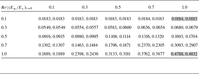
 Roeff
 Roeff

 ζ
 (EW/EV)t=0=1
 Ro=0.1
 Ro=1

 ζ
 Ro
 t

 ∇⋅v
 Ro=0.1
 (EW/EV)t=0
 t

 (EW/EV)t=0

 Ro=0.3
 (EW/EV)t=0=0.5
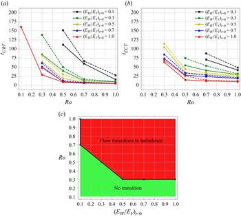
 a
 b
 c

 a
 |u^ω|
 h
 b
 |u^ω|
 Ro
 c
 f
 u^
 ω
 kh
 Ro

 ζ
 Ro
 h
 t=4π

 ∇⋅v
 Ro
 h
 t=4π

 E^
 Ro
 t=4π
 −16
 −2
 −16
 −2

 Ro=0.1
 1.0

 Ro

 Ro

 Ro

 Ro
 t

 Ro
 t

 Ro
 t



