1 Introduction
Brownian motion of micro- and nanoparticles is commonly encountered in many natural phenomena and engineering processes, such as materials and chemical engineering, aerosol diffusion in the atmosphere, biological medicine processes, etc. (Saffman & Delbrück Reference Saffman and Delbrück1975; Berna et al. Reference Berna, Leigh, Lubomska, Mendoza, Pérez, Rudolf and Zerbetto2005; Thompson & Wilson Reference Thompson and Wilson2016). Since Brownian motion was first explained by Einstein as the amplification of the thermal motion of the surrounding fluid molecules (Einstein Reference Einstein1905), many research works have been conducted to disclose the motion of nano- and microparticles in detail (Han et al. Reference Han, Alsayed, Nobili, Zhang, Lubensky and Yodh2006; Li et al. Reference Li, Kheifets, Medellin and Raizen2010; Huang et al. Reference Huang, Chavez, Taute, Luki, Jeney, Raizen and Florin2011).
The variation of the Brownian particle motion basically depends on the interacting molecular forces between the fluid and the particle. The frequency and magnitude of the forces determine the period of the ballistic motion and the magnitude of the velocity of the particle. However, it is impossible to make a direct measurement of these forces because of the limitation of the technological conditions. Another means to determine these forces is to make a full microscopic measurement of the particle movements, through which researchers can obtain the forces by interpreting the variation of the particle velocity (Li et al.
Reference Li, Kheifets, Medellin and Raizen2010; Pusey Reference Pusey2011). Previous research efforts have usually focused on the movement of the Brownian particles and its effect on the macroscopic diffusion processes, such as Einstein’s research on the macroscopic view and other research on the microscopic view. In the macroscopic view, Einstein established the connection between the mean displacement and the translational diffusion coefficient with statistical theory (Einstein Reference Einstein1905). Nowadays, researchers can obtain displacement resolution as small as 0.3 Å in space and as short as
 $0.01~\unicode[STIX]{x03BC}\text{s}$
in time intervals in the laboratory (Pusey Reference Pusey2011). The spatial and temporal resolution seemed to meet the demands for studying ballistic Brownian motion. Li et al. experimentally observed the ballistic regime of Brownian motion of suspended beads of glass in air and measured the instantaneous velocity of a Brownian particle (Li et al.
Reference Li, Kheifets, Medellin and Raizen2010). Huang et al. first captured the ballistic Brownian motion of a single particle suspended in liquid and studied the full transition from ballistic to diffusive Brownian motion (Huang et al.
Reference Huang, Chavez, Taute, Luki, Jeney, Raizen and Florin2011). Blum et al. (Reference Blum, Bruns, Rademacher, Voss, Willenberg and Krause2006) and Han et al. (Reference Han, Alsayed, Nobili, Zhang, Lubensky and Yodh2006) studied rotational and translational Brownian motion of non-spherical particles in water and rarefied gas respectively, etc. In spite of the exciting results achieved, further research with detectors of much higher spatial and temporal resolutions are still necessary, so that more detailed information of the particle velocity variation can be obtained for the force analysis.
In order to include the effect of the Brownian force on the particle motion in calculations, the classical Langevin equation (CLE) proposed by Langevin (Langevin Reference Langevin1908) was commonly used, which can be expressed as
 $$\begin{eqnarray}m\frac{\text{d}^{2}x}{\text{d}t^{2}}=-\unicode[STIX]{x1D701}\frac{\text{d}x}{\text{d}t}+F_{R}(t),\end{eqnarray}$$
where
 $m$
is the mass of Brownian particle,
 $x$
is the position of Brownian particle at
 $t$
time,
 $\unicode[STIX]{x1D701}$
is the Stokes coefficient of drag and
 $F_{R}(t)$
is the Brownian force which is commonly obtained from a certain stochastic allocation in white noise and no correlation in spatial and temporal space. Based on the Langevin equation for particle motion, Ermak and McCammon (Ermak & McCammon Reference Ermak and McCammon1978) developed the conventional algorithm for Brownian dynamic (BD) simulations. Their numerical method assumed that the properties of the random force in the particle equation of motion depend on the hydrodynamic interactions between the particles. The spatial displacement
 $x$
of a particle due to the Brownian motion and the diffusion coefficient
 $D$
for a spherical particle with radius
 $r$
moving in the fluid with viscosity coefficient
 $\unicode[STIX]{x1D702}$
was obtained
 $$\begin{eqnarray}\langle x^{2}\rangle =2Dt,\quad D=\frac{k_{B}T}{6\unicode[STIX]{x03C0}\unicode[STIX]{x1D702}r},\end{eqnarray}$$
where
 $k_{B}$
is the Boltzmann constant,
 $T$
is the absolute temperature. Brady and Bossis (Brady & Bossis Reference Brady and Bossis1988) developed a Stokesian dynamics technique for simulating the Brownian motion of many particles based on the Langevin equations. Unlike the approximations used by Ermak and McCammon (Ermak & McCammon Reference Ermak and McCammon1978), they computed the hydrodynamic interactions through a grand resistance tensor. Thus the properties of the random force in the particle equations depend on the grand resistance tensor, which in turn depends on the particle positions, shapes and the fluid properties. The CLE is an empirical equation which was derived based on the macroscopic diffusion process resulting from the Brownian motion. Although the CLE has been widely used in many engineering calculations, it is hard to determine the accuracy when describing the Brownian force with this equation.
In this paper, the properties of the random Brownian force, such as the frequency of the force acting on the nanoparticle and the effect of the particle size on the force, are studied with the molecular dynamics simulation. In the simulation, the nitrogen (N
 $_{2}$
) molecules are adopted as the fluid surrounding the silver Brownian particle. A wide range of
 $1/Kn=R/\unicode[STIX]{x1D706}$
numbers are taken into consideration in the numerical investigation.
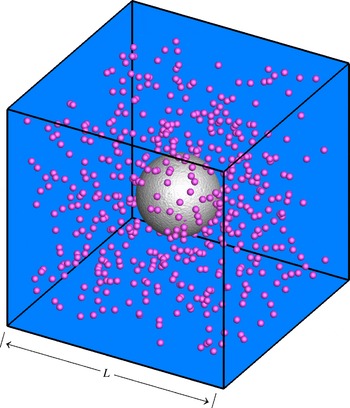
Schematic computational domain of Ag particle in N
 $_{2}$
environment.

2 Numerical simulation
A silver (Ag) particle with a radius of
 $R=40$
nm is fixed at the centre of the cubic computational zone (as shown in figure 1). The particle is constructed from an face centered cubic (FCC) silver crystal and by truncating atoms that lie outside of the sphere of the radius
 $R$
. Due to the large ratio between the particle diameter and the gas molecule diameter, the N
 $_{2}$
molecule is simplified to a single sphere and the rotation is neglected. The detailed arrangement of the simulation can also refer to Li’s research (Li & Wang Reference Li and Wang2005), in which the interaction between the free nitrogen molecules and the atoms of a silver particle was studied. As described in Li & Wang (Reference Li and Wang2005), the rotation of the N
 $_{2}$
molecule inevitably leads to collision dynamics more complex than those assumed here, but this does not apparently affect the forces acting on the Ag particle.
Both the interactions between the N
 $_{2}$
molecules and the interactions between N
 $_{2}$
molecules and Ag atoms are all simulated with the Lennard–Jones 12-6 potential function
 $$\begin{eqnarray}U_{LJ}(r)=\left\{\begin{array}{@{}ll@{}}4\unicode[STIX]{x1D700}\left(\left({\displaystyle \frac{\unicode[STIX]{x1D70E}}{r}}\right)^{12}-\left({\displaystyle \frac{\unicode[STIX]{x1D70E}}{r}}\right)^{6}\right), & r<r_{c}\\ 0, & r\geqslant r_{c},\end{array}\right.\end{eqnarray}$$
where
 $\unicode[STIX]{x1D700}$
is the well depth,
 $\unicode[STIX]{x1D70E}$
is the collision diameter,
 $r$
is the separation distance and
 $r_{c}$
is the cutoff distance equal to
 $2.5\unicode[STIX]{x1D70E}$
. In this paper, the coefficients
 $\unicode[STIX]{x1D700}_{g}/k_{B}=98.4~\text{K}$
,
 $\unicode[STIX]{x1D70E}_{g}=3.652$
Å,
 $\unicode[STIX]{x1D700}_{p}/k_{B}=3995.4~\text{K}$
and
 $\unicode[STIX]{x1D70E}_{p}=2.54$
Å are adopted (Li & Wang Reference Li and Wang2003). The subscripts
 $g$
and
 $p$
denote the nitrogen molecule and silver atom respectively.
 $k_{B}$
is the Boltzmann constant. A tight-binding potential function (Cleri & Rosato Reference Cleri and Rosato1993) for interactions between the Ag atoms is used
 $$\begin{eqnarray}\displaystyle & \displaystyle E_{c}=\mathop{\sum }_{i}(E_{R}^{i}+E_{B}^{i}), & \displaystyle\end{eqnarray}$$
 $$\begin{eqnarray}\displaystyle & \displaystyle E_{R}^{i}=\mathop{\sum }_{j}A_{\unicode[STIX]{x1D6FC}\unicode[STIX]{x1D6FD}}\text{e}^{-p_{\unicode[STIX]{x1D6FC}\unicode[STIX]{x1D6FD}}(r_{ij}/r_{0}^{\unicode[STIX]{x1D6FC}\unicode[STIX]{x1D6FD}}-1)}, & \displaystyle\end{eqnarray}$$
 $$\begin{eqnarray}\displaystyle & \displaystyle E_{B}^{i}=-\left(\mathop{\sum }_{j}\unicode[STIX]{x1D709}_{\unicode[STIX]{x1D6FC}\unicode[STIX]{x1D6FD}}^{2}\text{e}^{-2q_{\unicode[STIX]{x1D6FC}\unicode[STIX]{x1D6FD}}(r_{ij}/r_{0}^{\unicode[STIX]{x1D6FC}\unicode[STIX]{x1D6FD}}-1)}\right)^{1/2}, & \displaystyle\end{eqnarray}$$
 $r_{ij}$
is the distance between atoms
 $i$
and
 $j$
,
 $r_{0}^{\unicode[STIX]{x1D6FC}\unicode[STIX]{x1D6FD}}$
represents the first-neighbours distance in the
 $\unicode[STIX]{x1D6FC}\unicode[STIX]{x1D6FD}$
lattice.
 $A,\unicode[STIX]{x1D709},p,q$
are the free parameters for Ag atoms and are respectively equal to 0.1028 eV, 1.178 eV, 10.928 and 3.139.
The simulations are performed in the
 $(N_{0}+M_{0},V,T)$
ensemble, in which
 $N_{0}$
nitrogen molecules and
 $M_{0}$
silver atoms are included. The temperature is kept at 300 K with a Berendsen thermostat (Berendsen et al.
Reference Berendsen, Postma, van Gunsteren, Dinola and Haak1984), and a fixed boundary condition is used.
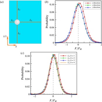
In order to eliminate the influence of the boundary on the numerical results, different sizes of the computational domain, namely the distances between the particle and the boundary, are tested. As shown in figure 2(a), a silver particle is placed inside the computational domain with its distance to the boundary at
 $L_{2}=20\unicode[STIX]{x1D706}$
so that the boundary effect can be neglected, except for the distance
 $L_{1}$
which is on the left side in the
 $x$
direction. Figure 2(b) shows the probability distribution of the resultant force sampled at every time step in the
 $x,y$
and
 $z$
directions, respectively, with the condition of the distance
 $L_{1}=\unicode[STIX]{x1D706}$
, where the mean path
 $\unicode[STIX]{x1D706}$
is calculated as
 $$\begin{eqnarray}\unicode[STIX]{x1D706}=\frac{1}{\sqrt{2}\unicode[STIX]{x03C0}\text{d}^{2}n},\end{eqnarray}$$
where
 $d$
is the effective diameter of a nitrogen molecule which equals 4.8 Å in the present paper and
 $n$
is the number of nitrogen molecules per unit volume. The mean intensity of the force is calculated as
 $$\begin{eqnarray}F_{M}=\frac{C}{N_{c}}\mathop{\sum }_{i}^{N_{c}}|F_{i}|,\end{eqnarray}$$
where
 $F_{i}$
is the transient force acting on the particle at time step
 $i$
and
 $N_{c}$
is the number of all the time steps in the computational period. If
 $C=1$
,
 $F_{M}$
is the mean magnitude of the force acting on the particle. When
 $C\approx 1.25$
, it is found the dimensionless force
 $F/F_{M}$
conforms to the standard Gaussian distribution where the standard deviation is 1. Thus
 $C=1.25$
is adopted in the current paper.
The distributions of the force components in the
 $y$
and
 $z$
directions are both standard normal distributions in which the mean value is 0, but the mean value in the
 $x$
direction apparently deviates from 0. The difference may result from the boundary effect because of the small value of
 $L_{1}$
. If the distance
 $L_{1}$
is improved and the mean path of the N
 $_{2}$
molecules is constant, the boundary effect weakens and the mean value of the force components in the
 $x$
direction return to 0 when
 $L_{1}\geqslant 3\unicode[STIX]{x1D706}$
(as shown in figure 2
c). In this paper, a distance of
 $3\unicode[STIX]{x1D706}$
between the particle and the boundary of the computational domain is adopted, so that the boundary effect can be considered negligible.
Boundary effect test. (a) Schematic computational domain, (b) probability distribution of force components in the
 $x$
,
 $y$
and
 $z$
directions for
 $L_{1}=\unicode[STIX]{x1D706}$
, (c) probability distribution of force component in the
 $x$
direction for different
 $L_{1}/\unicode[STIX]{x1D706}$
.

In this work, a series of
 $1/Kn(1/Kn=R/\unicode[STIX]{x1D706})$
numbers varying from 0.1 to 400 are adopted by changing the nitrogen pressure. Beeman’s leapfrog algorithm (Beeman Reference Beeman1976), which can keep the momentum of the system constant, is used for integration of the equations of motion, with a time step of 1 fs. Research shows that the time step of relaxation in the computation is mainly influenced by the number density of molecules, the
 $1/Kn$
number and the initial state point. Approximately 1
 ${\sim}$
20 million time steps of relaxation are conducted for different
 $1/Kn$
numbers in the present paper (Vorholz et al.
Reference Vorholz, Harismiadis, Rumpf, Panagiotopoulos and Maurer2000). After the computational system reaches its steady state, the results start to be recorded. The calculations are carried out on a workstation with a graphics processing unit (GPU) card of Tesla K40.
3 Results and discussion
3.1 Validation of the results
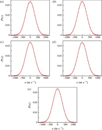
In the canonical ensemble, the molecular velocity conforms to the standard normal distribution. Figure 3(a–c) shows the distribution of the N
 $_{2}$
molecular velocity component in the
 $x$
direction at different times. The definite Gaussian distributions are clearly displayed at all times. Figure 3(d,e) shows the distributions of the velocity components in the
 $y$
and
 $z$
directions, respectively. The Gaussian distributions of the velocity can also be clearly observed. The same distribution in the three directions shows the isotropy of the molecular motion. According to Tobias, Martyna & Klein (Reference Tobias, Martyna and Klein1993), the simulations in the present work can realize the thermodynamic limit, and the results are effective and feasible.
Probability distribution of N
 $_{2}$
molecular velocity (a) velocity component in the
 $x$
direction at
 $t=50~\text{ps}$
, (b) velocity component in the
 $x$
direction at
 $t=100~\text{ps}$
, (c) velocity component in the
 $x$
direction at
 $t=150~\text{ps}$
, (d) velocity component in the
 $y$
direction at
 $t=50~\text{ps}$
, (e) velocity component in the
 $z$
direction at
 $t=50~\text{ps}$
.

3.2 Probability distribution of the force
After the forces acting on the particle are sampled every time step for
 $10^{6}$
time steps, the probability distributions of the force components in the
 $x$
,
 $y$
and
 $z$
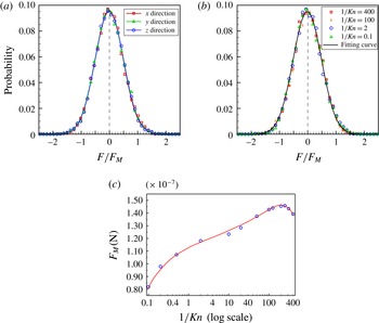
directions determined, as shown in figure 4, respectively.
It can be observed that no obvious difference in the probability distribution of the forces is found between the three components in the
 $x$
,
 $y$
and
 $z$
directions (as shown in figure 4
a). Thus, only the force component in the
 $x$
direction is used in the following analysis. Figure 4(b) shows the probability distribution of the forces for different
 $1/Kn$
numbers. The self-similarity in the probability distribution of the dimensionless force
 $F/F_{M}$
can be found for different
 $1/Kn$
numbers. As described above, the probability distribution of
 $F/F_{M}$
obeys the standard Gaussian distribution
 $$\begin{eqnarray}P(x)=\frac{1}{\sqrt{2\unicode[STIX]{x03C0}}\unicode[STIX]{x1D70E}_{1}}\text{e}^{-2(x^{2}/\unicode[STIX]{x1D70E}_{1}^{2})},\end{eqnarray}$$
where the standard deviation
 $\unicode[STIX]{x1D70E}_{1}$
is 1.
Probability distribution of the Brownian forces (a) force components in the
 $x$
,
 $y$
and
 $z$
directions for
 $1/Kn=2$
, (b) force components in the
 $x$
direction for different
 $1/Kn$
numbers, (c) the
 $1/Kn$
number-dependent change of the
 $F_{M}$
in log scale.

Figure 4(c) shows the non-monotonic variation process of
 $F_{M}$
with
 $1/Kn$
. It can be obviously observed that, as the
 $1/Kn$
number grows,
 $F_{M}$
first increases and then decreases after it reaches a maximum value at
 $1/Kn\approx 250$
. This variation process explicitly exhibits the size effect on the mean intensity of the force acting on the particle. The decreasing process of the mean force intensity for
 $1/Kn>250$
in the present work is consistent with the Langevin model, which was also verified in the experimental observation, e.g. Han et al. experimentally found that ellipsoidal particle diffuses more rapidly along its long axis than along its short axis (Han et al.
Reference Han, Alsayed, Nobili, Zhang, Lubensky and Yodh2006). The
 $1/Kn$
number in their experiments was far greater than
 $250$
. Because the cross-sectional area in the long axial direction is smaller than that in the short axial direction, the force in the long axial direction is correspondingly larger. But for
 $1/Kn<250$
, the increasing process of the mean force intensity observed in the present work has not been reported in previous research to date. This phenomenon can be explained based on the assumption of the limits
 $1/Kn=0$
and
 $1/Kn\rightarrow \infty$
. If
 $1/Kn=0$
, no gas molecule acts on the particle and the force becomes zero. If
 $1/Kn\rightarrow \infty$
, numerous gas molecules uniformly act on the surface of the particle at the same time, and the resultant force equals zero too. Thus the variation tendency in the present paper between the two limits can be easily obtained. The mean intensity of the force depends on the force balance around the surface of the particle and the number of interactions between the molecule and the particle atoms. When
 $1/Kn\rightarrow \infty$
and the force balance is the dominant factor, the mean intensity of the force decreases, and when
 $1/Kn=0$
and the number of interactions is the dominant factor, the mean intensity of the force increases.
3.3 Frequency distribution of the force
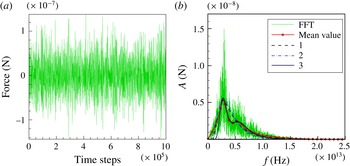
Figure 5 shows the time-dependent variation and the frequency spectrum distribution of the force in the case of
 $1/Kn=0.1$
. A white-noise-like temporal evolution can be found, which conforms to our original impression of Brownian motion (figure 5
a). However, the frequency spectrum distribution of the forces obtained with fast Fourier transform exhibits a shape similar to the gamma distribution or the logarithmic normal distribution (figure 5
b). In order to make a clear observation, the mean value of the amplitude
 $\langle A(f)\rangle$
in the frequency interval
 $\unicode[STIX]{x1D6FF}f$
is defined as
 $$\begin{eqnarray}\langle A(f_{0})\rangle =\frac{1}{2N}\mathop{\sum }_{i=-N}^{N}A\left(f_{0}+\frac{i}{2N}\unicode[STIX]{x1D6FF}f\right).\end{eqnarray}$$
If a function based on the gamma distribution is used to fit the mean amplitude for different frequencies, which is shown as curve 1 in figure 5(b), then
 $$\begin{eqnarray}\langle A(f)\rangle =C_{1}\frac{\unicode[STIX]{x1D6FD}^{\unicode[STIX]{x1D6FC}}f^{\unicode[STIX]{x1D6FC}-1}\text{e}^{-\unicode[STIX]{x1D6FD}f}}{\unicode[STIX]{x1D6E4}(\unicode[STIX]{x1D6FC})},\end{eqnarray}$$
where the coefficient
 $C_{1}=7.7143\times 10^{4}$
,
 $(\unicode[STIX]{x1D6FD}^{\unicode[STIX]{x1D6FC}}f^{\unicode[STIX]{x1D6FC}-1}\text{e}^{-\unicode[STIX]{x1D6FD}f}/\unicode[STIX]{x1D6E4}(\unicode[STIX]{x1D6FC}))$
is the gamma distribution function where
 $\unicode[STIX]{x1D6FC}=1.2375\times 10^{13}$
,
 $\unicode[STIX]{x1D6FD}=4.5$
. When the logarithmic normal distribution is used, the function can be expressed as (shown as curve 2 in figure 5
b)
 $$\begin{eqnarray}\langle A(f)\rangle =\frac{C_{2}}{f\unicode[STIX]{x1D70E}_{1}\sqrt{2\unicode[STIX]{x03C0}}}\text{e}^{-((ln\,f-\unicode[STIX]{x1D707}_{1}/\unicode[STIX]{x1D70E}_{1})^{2})/2},\end{eqnarray}$$
where the coefficient
 $C_{2}=2.175\times 10^{4}$
,
 $1/f\unicode[STIX]{x1D70E}_{1}\sqrt{2\unicode[STIX]{x03C0}}\text{e}^{-((ln\,f-\unicode[STIX]{x1D707}_{1}/\unicode[STIX]{x1D70E}_{1})^{2})/2}$
is the log-normal distribution function where
 $\unicode[STIX]{x1D707}_{1}=28.9234$
,
 $\unicode[STIX]{x1D70E}_{1}=0.5$
. In fact, the variation of the mean amplitude is not very smooth with frequency, oscillations can be easily observed. It is found that the peaks of the oscillations usually occur at an integer multiple of the preferential frequency. Meanwhile, the intensity of the oscillations decays rapidly and only the first two peaks can be easily observed. This implies that such periodic oscillations may result from the strongest interaction between the gas molecules and the particle at the preferential frequency. When the superposition of the periodic oscillations is considered in the logarithmic normal distribution form, the function can be expressed as (shown as curve 3 in figure 5
b)
 $$\begin{eqnarray}\langle A(f)\rangle =\mathop{\sum }_{i=1}\frac{0.4^{(\text{i}-1)^{1.6}}C_{3}}{(f/i)\unicode[STIX]{x1D70E}_{2}\sqrt{2\unicode[STIX]{x03C0}}}\text{e}^{-((\ln (f/i)-\unicode[STIX]{x1D707}_{2}/\unicode[STIX]{x1D70E}_{2})^{2})/2},\end{eqnarray}$$
where the coefficient
 $C_{3}=1.188\times 10^{4}$
,
 $\unicode[STIX]{x1D707}_{2}=28.823$
,
 $\unicode[STIX]{x1D70E}_{2}=0.24$
.
Such a frequency spectrum distribution implies that the variation of the particle velocity would be most intensive within a certain range of frequency, which cannot be correctly described with the commonly used Langevin model. Experimental observation of the particle motion in such ranges of the frequency is far beyond the capability of current detectors whose time resolution usually reaches
 $1\times 10^{-8}~\text{s}$
. Thus the non-uniform frequency distributed ballistic motion is difficult determine in experiment. Strictly speaking, most of the published experimentally observed ballistic motions are not really ballistic, they are quasi-ballistic motion (Huang et al.
Reference Huang, Chavez, Taute, Luki, Jeney, Raizen and Florin2011; Pusey Reference Pusey2011).
Brownian force for
 $1/Kn=0.1$
. (a) Temporal variation of the force and (b) frequency spectrum distribution.
 $f$
is the frequency and A is the amplitude. Curve 1 is the gamma distribution based function; curve 2 is the log-normal distribution based function; curve 3 is the log-normal distribution based function including the periodic oscillation.

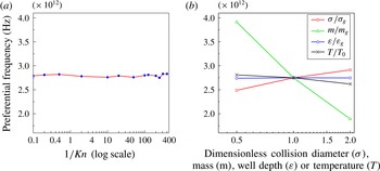
Preferential frequency of the force: (a) preferential frequency variation with
 $1/Kn$
, (b) preferential frequency variation with physical properties when
 $1/Kn=2$
.
 $\unicode[STIX]{x1D70E}_{g}$
is the collision diameter of nitrogen,
 $\unicode[STIX]{x1D700}_{g}$
the well depth of nitrogen,
 $m_{g}$
the mass of nitrogen and
 $T_{0}=300~\text{K}$
.

Similar spectrum distributions can also be found for different values of the
 $1/Kn$
and further research is still needed to find the reason for this kind of frequency spectrum distribution. It may result from the interaction between the atoms of the solid particles and the gas molecules. Figure 6 shows the change of the preferential frequency where the peak amplitude of the Brownian force appears. It can be found that the preferential frequencies do not change obviously for different values of
 $1/Kn$
(as shown in figure 6
a). Further research shows that the preferential frequency can vary with some physical properties of the gas molecules, such as the collision diameter, well depth, mass and temperature, etc. Figure 6(b) shows the variation of the preferential frequency for
 $1/Kn=2$
. Of all the factors tested in the current research, the mass has the greatest impact on the preferential frequency. The collision diameter and the temperature also affect the priority frequency. The well depth has little effect on it.
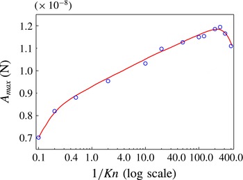
Although the preferential frequencies where the peak amplitude appears do not change obviously for different
 $1/Kn$
numbers, the peak value of the mean amplitude
 $A_{max}$
differs greatly. Apparent change of
 $A_{max}$
can be found for different
 $1/Kn$
numbers. Further analysis shows that the changing process is not monotonic (as shown in figure 7). Similar to the variation of the mean intensity of the forces,
 $A_{max}$
first increases dramatically before its growth rate gradually decreases and finally
 $A_{max}$
decreases after it reaches the maximum value at
 $1/Kn\approx 250$
. The results are consistent with the variation of the mean intensity of the forces
 $F_{M}$
shown in figure 4(c). Both the peak value of the mean amplitude in the frequency spectrum distribution and the mean intensity of the force prove the size effect (the radius of the particle or the mean free path of the molecules) of the Brownian force acting on the particle.
The
 $1/Kn$
number-dependent variation of the peak value of the mean amplitude.

In order to undertake a validation test on the obtained force spectrum distribution, a much longer term of time-dependent force variation is deducted based on the current spectrum distribution
 $$\begin{eqnarray}F(t)=\mathop{\sum }_{j}[a_{j}\cos (f_{j}t)+\text{i}b_{j}\sin (f_{j}t)],\end{eqnarray}$$
where
 $F$
is the force acting on the particle at time
 $t$
, i is the imaginary unit and
 $f$
is the frequency.
 $a$
and
 $b$
are the coefficients of the real and imaginary parts, respectively, where
 $A^{2}=a^{2}+b^{2}$
. The force variation during the period
 $0\sim 30~\unicode[STIX]{x03BC}\text{s}$
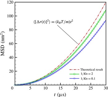
is deducted and the mean square displacements of the Brownian motion of a free silver particle (
 $m=3.1\times 10^{-14}~\text{kg}$
) are obtained with
 $T=300~\text{K}$
(as shown in figure 8)
 $$\begin{eqnarray}\langle [\unicode[STIX]{x0394}r(\unicode[STIX]{x1D70F})]^{2}\rangle =\frac{1}{\unicode[STIX]{x1D70F}_{tot}-\unicode[STIX]{x1D70F}}\mathop{\sum }_{\unicode[STIX]{x1D70F}=1}^{\unicode[STIX]{x1D70F}_{tot}-\unicode[STIX]{x1D70F}}[r(\unicode[STIX]{x1D70F}_{0}+\unicode[STIX]{x1D70F})-r(\unicode[STIX]{x1D70F}_{0})]^{2},\end{eqnarray}$$
where
 $\unicode[STIX]{x1D70F}$
is time step number,
 $\unicode[STIX]{x1D70F}_{0}$
the start time step and
 $\unicode[STIX]{x1D70F}_{tot}$
total sampling time steps. The predicted results agree well with the theoretical result. Similar results were also obtained in the experimental studies finished by Li et al., their experimental results were also a little less than theoretical result (Li et al.
Reference Li, Kheifets, Medellin and Raizen2010).
The mean square displacements of the particles Brownian motion for different
 $1/Kn$
numbers.

4 Conclusions
Brownian forces acting on nanoparticles are numerically investigated with the molecular dynamics method. Some new phenomena are disclosed.
-
(i) The probability distribution shows that the Brownian forces conform to the Gaussian distribution. Self-similarity of the probability distribution of the Brownian forces for different
 $1/Kn$
numbers is found.
-
(ii) The frequency spectrum distribution shows that the Brownian forces are not white noise, which is different from the assumption used in the Langevin model. The preferential frequency of the Brownian force is found.
-
(iii) The size effect, such that the Brownian force is not monotonically varying with
$1/Kn=R/\unicode[STIX]{x1D706}$
, is also found. It increases first and then decreases after it reaches a maximum value at
$1/Kn\approx 250$
.


Acknowledgements
The authors gratefully acknowledge the financial support of Natural Science Fund of China (grant no: 51390490, 11132008), National key research and development program of China (grant no: 2016YFB0600101) and Zhejiang Province Science and Technology Innovation Team Project (2013TD18).