


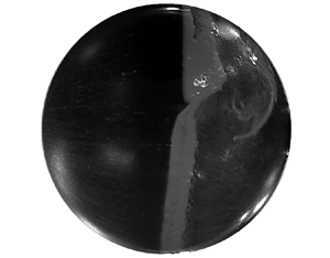





1. Introduction
Flow past a sphere has been widely studied owing to its simple geometry and, yet, embodying the rich and complex phenomena associated with bluff body flows. The governing parameter for this flow is the Reynolds number,  $Re={U_{\infty } D}/{\nu }$, where
 $U_{\infty }$ is the free stream speed,
 $D$ is the diameter of the sphere and
 $\nu$ is the kinematic viscosity. When the boundary layer over a bluff body undergoes transition from laminar to turbulent, a steep drop in drag force is observed with increasing
 $Re$. This phenomenon is known as the drag crisis (Roshko Reference Roshko1961; Achenbach Reference Achenbach1968). It has been studied extensively for flow past a cylinder and a sphere.
Achenbach (Reference Achenbach1972) carried out a comprehensive study for flow past a sphere. Based on the state of the boundary layer, he proposed classification of the flow into four regimes. In the subcritical regime, the laminar boundary layer separates upstream of the shoulder. The drag coefficient in this regime is nearly independent of  $Re$. Drag crisis takes place in the critical regime. In the supercritical regime, the point of transition of boundary layer moves upstream with increasing
 $Re$ and drag coefficient gradually increases. The transcritical regime is characterised by movement of the transition point from the shoulder towards the front stagnation point and rapid increase in the drag coefficient. However, these attributes do not translate into clear boundaries between adjacent regimes. Schewe (Reference Schewe1983) defined the regimes of the flow past a cylinder based on the mean drag force. He proposed that the
 $Re$ at which drag force is maximum may be considered to be the boundary between subcritical and critical regimes, whereas the
 $Re$ at which drag force is minimum is the boundary between critical and supercritical regimes. These definitions lead to sharp and unambiguous boundaries between successive regimes. These were extended for flow past a sphere by Deshpande et al. (Reference Deshpande, Kanti, Desai and Mittal2017).
One of the interesting flow features in the subcritical flow past a cylinder is a secondary recirculation bubble downstream of the point of laminar separation. It was first reported by Son & Hanratty (Reference Son and Hanratty1969), who referred to it as secondary vortex. Cheng et al. (Reference Cheng, Pullin, Samtaney, Zhang and Gao2017) also observed the secondary vortex in the subcritical regime in their wall-resolved large eddy simulations (LES). Secondary vortex was also reported in the supercritical regime ( $Re=6 \times 10^5$) by Ono & Tamura (Reference Ono and Tamura2008). Recently, Chopra & Mittal (Reference Chopra and Mittal2022) numerically investigated the flow past a cylinder for a range of
 $Re$ spanning subcritical, critical and supercritical regimes. They observed the secondary vortex in all three regimes. In the subcritical regime, the footprint of secondary vortex was observed to increase with increase in
 $Re$ for
 $5 \times 10^3 \leq Re \leq 4 \times 10^4$ and decrease thereafter. A slight decrease was observed in the critical and supercritical regimes. For the flow past a sphere, the existence and development of a secondary vortex has not been investigated previously, to the best of our knowledge.
The laminar boundary layer over a sphere undergoes early separation due to an adverse pressure gradient. The separated shear layer becomes unstable some distance downstream and rolls up into small vortices (Williamson Reference Williamson1996). The location of the onset of instability moves upstream with increase in  $Re$. In the critical regime, these vortices lead to mixing of the flow in the boundary layer, thereby energising it. The energised boundary layer reattaches to the surface and the final separation takes place farther downstream (Singh & Mittal Reference Singh and Mittal2005). The delayed separation leads to a narrower wake and significantly smaller drag coefficient (Fage Reference Fage1936; Suryanarayana & Prabhu Reference Suryanarayana and Prabhu2000; Jeon et al. Reference Jeon, Choi, Jeon, Choi and Park2004). The recirculation region formed between laminar separation and turbulent reattachment is called the laminar separation bubble (LSB). The presence of a LSB over a sphere in critical regime has been observed in past studies via surface pressure measurements (Fage Reference Fage1936; Achenbach Reference Achenbach1972; Deshpande et al. Reference Deshpande, Kanti, Desai and Mittal2017), skin friction measurements (Achenbach Reference Achenbach1972) and oil flow visualisations (Raithby & Eckert Reference Raithby and Eckert1968; Taneda Reference Taneda1978; Deshpande et al. Reference Deshpande, Kanti, Desai and Mittal2017).
For a cylinder in the critical regime, LSB is known to appear/disappear intermittently in time (Miau et al. Reference Miau, Tsai, Lin, Tu, Fang and Chen2011; Cadot et al. Reference Cadot, Desai, Mittal, Saxena and Chandra2015; Chopra & Mittal Reference Chopra and Mittal2017). Similar intermittent behaviour of the LSB has also been reported on a sphere leading to large unsteadiness in drag force (Torii et al. Reference Torii, Isobe, Horikoshi and Miura1981; Norman & McKeon Reference Norman and McKeon2011). Deshpande et al. (Reference Deshpande, Kanti, Desai and Mittal2017) investigated the dynamics of the LSB in the critical regime in detail and proposed further division of the critical regime into three subregimes based on the presence and behaviour of the LSB. In subregime I, the boundary layer undergoes laminar separation and the flow is devoid of the LSB. The drag coefficient in this subregime decreases gradually due to the increase in base pressure and suction upstream of the shoulder. Subregime II is characterised by intermittent appearance/disappearance of the LSB. The frequency of appearance of the LSB and the duration of its stay increase with increasing  $Re$. In subregime III, LSB is observed at all times and drag coefficient decreases due to increasing base pressure. They also concluded that for the smooth model employed in their study and exposed to very low free stream turbulence (FST), the LSB is axisymmetric, i.e. it appears and disappears at all azimuthal locations simultaneously.
The transition of boundary layer as well as the vortex shedding in the wake of a bluff body is extremely sensitive to FST (Bearman & Morel Reference Bearman and Morel1983; Norberg & Sunden Reference Norberg and Sunden1987). The most prominent effect of FST is reduction in the critical  $Re$ for the onset of the drag crisis (Raithby & Eckert Reference Raithby and Eckert1968; Moradian, Ting & Cheng Reference Moradian, Ting and Cheng2009; Son et al. Reference Son, Choi, Jeon and Choi2010; Desai, Shakya & Mittal Reference Desai, Shakya and Mittal2021). In presence of FST, suppression of vortex shedding in the wake of the sphere at subcritical
 $Re$ was observed experimentally by Tyagi et al. (Reference Tyagi, Liu, Ting and Johnston2006) and computationally by Rodriguez, Lehmkuhl & Soria (Reference Rodriguez, Lehmkuhl and Soria2021). Raithby & Eckert (Reference Raithby and Eckert1968) found that not only the drag crisis take place at a lower
 $Re$, but it also becomes gradual with increasing FST. Son et al. (Reference Son, Choi, Jeon and Choi2010) studied the drag crisis over a sphere for three different levels of FST:
 $4\,\%$,
 $6\,\%$ and
 $8\,\%$. They observed that with increasing FST, the laminar separation shifts downstream whereas the locations of turbulent reattachment and turbulent separation remain unchanged, causing
 $\overline {C}_D$ to be nearly constant after the drag crisis for different levels of FST.
Although the effects of FST on drag force in the subcritical regime and on the onset of drag crisis have been investigated in depth, the effect of FST on the dynamics of the LSB has not received adequate attention. As the flow is extremely sensitive to small disturbances, measurements in different wind tunnels are affected by the FST level of the tunnel. Therefore, the effect of low FST ( $T_u \leq 1\,\%$) on these dynamics is of particular interest. To this end, we attempt to answer the following questions in the present study. (i) How does low FST affect the drag crisis? (ii) As is known for a cylinder, does a secondary vortex exist in the high subcritical regime for low FST for a sphere as well? (iii) Is the formation of the LSB in the critical regime always axisymmetric, i.e. does the LSB form at all azimuthal locations simultaneously? (iv) What are the various intermittent flow states in the critical regime and how do they evolve with increasing
 $Re$? (v) How does FST affect the topology of LSB? To explore these questions, experiments are carried out on flow past a sphere in the range
 $5 \times 10^4 \leq Re \leq 5\times 10^5$ and subjected to five different turbulence intensities ranging from
 $0.06\,\%$ to
 $1.36\,\%$. Unsteady force and pressure measurements are utilised to understand the dynamics of LSB and oil flow visualisations are used for a qualitative understanding of the flow.
2. Experimental set-up and methodology
Experiments were carried out at National Wind Tunnel Facility, IIT Kanpur. It is a closed circuit, atmospheric facility with a test section of  $2.25\,{\rm m}\times 3$ m size. Maximum wind speed achievable in the tunnel is 80 m s
 $^{-1}$. For the present study, the speed range
 $10\,{\rm m}\,{\rm s}^{-1}\leq U_{\infty }\leq 70\,{\rm m}\,{\rm s}^{-1}$ was utilised. The turbulence intensity was found to not exceed
 $0.06\,\%$ for this speed range. More details on the characterisation of this wind tunnel can be found in Cadot et al. (Reference Cadot, Desai, Mittal, Saxena and Chandra2015).
Figure 1 shows a schematic of the set-up and the coordinate system. The sphere used for force measurements had a diameter of 120 mm and was manufactured using stereo-lithography technique with Acura 60 material. After fabrication and post-processing, the model was polished and painted black to obtain glossy smooth finish. Surface roughness of the finished model was measured using Surftest SJ-301 surface roughness tester from Mitutoyo Corporation. The maximum surface roughness was found to be  $k/D = 3.8 \times 10^{-6}$. Thus, the sphere can be considered to be smooth as per the classification proposed by Achenbach & Heinecke (Reference Achenbach and Heinecke1981). The sphere was made up of two interlocking parts. The seam resulting at the boundary of these two parts lies at a polar location of
 $\theta = 130^{\circ }$ from the front stagnation point. This ensured that this seam did not interfere with the transition of the boundary layer. The sphere was mounted on a horizontal sting of diameter 25 mm and length 450 mm. The horizontal sting was mounted on a vertical support which was grounded to the tunnel floor. The cross section of the tunnel is
 $2.25\,{\rm m}\times 3$ m whereas the frontal area presented by the model is 0.0113 m
 $^2$. The resulting blockage ratio is
 $0.17\,\%$. It is very small, suggesting that effect of blockage is negligible. The model and set-up were similar to those used by Deshpande et al. (Reference Deshpande, Kanti, Desai and Mittal2017), to which the reader may refer for a more detailed description.
(a) Schematics of model mounting in the wind tunnel. Experimental set-up for (b) force measurements and (c) pressure measurements.

A six-component strain-gauge-based force balance was used for unsteady force measurement. Strain-gauge-based sensors are inherently linear and have wide frequency response (Harris & Piersol Reference Harris and Piersol2002). They have been employed for measurement of time-varying forces by a number of researchers (Suryanarayana & Prabhu Reference Suryanarayana and Prabhu2000; Deshpande et al. Reference Deshpande, Kanti, Desai and Mittal2017; Shah, Shakya & Mittal Reference Shah, Shakya and Mittal2019). The balance was installed inside the horizontal sting and connected directly to the rear part of the sphere. The calibration curve of the balance was linear. Output signals from the balance were amplified via an eight-channel NI-SCXI-1520 signal conditioning unit. The low-pass filter cut-off was set at 100 Hz and force data were acquired at a sampling rate of 500 Hz. At least 60 s of data were acquired at each speed in the subcritical and supercritical regimes. This results in  $tU_{\infty }/D > 6000$ at all speeds, well above the
 $tU_{\infty }/D \approx 2000$ suggested by Norman & McKeon (Reference Norman and McKeon2011) for convergence of mean force coefficients. At least 120 s of data were acquired at each speed in the critical regime to capture sufficient instances of long-period fluctuations associated with intermittent switching of states. Despite the wide frequency response of strain gauge sensors, the force balance set-up is limited by its relatively low natural frequencies. Therefore, a moving average of suitable time period, analogous to a low-pass filter, was utilised. Moving average is described in detail in § 2.2. The non-dimensionalised force coefficients in the three directions are indicated by
 $C_D$,
 $C_Y$ and
 $C_Z$, respectively. The uncertainties in force coefficients decrease progressively with increase in speed. At the lowest
 $Re$ for which measurements were conducted (
 $Re=1\times 10^5$), uncertainties in
 $C_D$,
 $C_Y$ and
 $C_Z$ were estimated to be
 ${\pm }0.02$,
 ${\pm }0.02$ and
 ${\pm }0.03$ respectively.
Another sphere of identical geometry and smoothness was used for pressure measurements. This model had 63 pressure ports drilled normal to the surface of the sphere and placed along splines to avoid interference with each other. Figure 2 shows the distribution of these pressure ports. Twenty-five pressure ports were located along splines  $E$ and
 $W$ each, between
 $15^{\circ } \leq \theta \leq 150^{\circ }$. For finer spatial resolution in the region where LSB forms, 13 of these ports were located in the range
 $90^{\circ }\leq \theta \leq 126^{\circ }$. Along splines
 $N$ and
 $S$ each, 6 ports were located in the range
 $90^{\circ }\leq \theta \leq 105^{\circ }$. One port was located at the front stagnation point, i.e. at
 $\theta = 0^{\circ }$. Four ports were drilled on the sting, close to the region of
 $\theta =180^{\circ }$, to measure the base pressure. The value reported in this study is the average from these four ports.
Schematics showing the locations of pressure ports along different splines on the surface of the sphere: (a) isometric view and (b) front view. Dashed and dotted lines indicate the intersection of the sphere with  $xy$ and
 $xz$ planes, respectively. The origin of the coordinate axes lies at the centre of the sphere. It is shifted outside the sphere in (a) to show the orientation of axes.

Pressure from the ports was measured using three ESP scanners of range  $-2500$ to
 $+2500$ Pa. Two scanners were installed inside the model and firmly glued to the supports using double sided tape. Pressure ports on the surface of the sphere were connected to these two scanners. Base pressure, static pressure and total pressure in the tunnel were measured using another scanner kept outside the tunnel. The scanners had a resolution of
 ${\pm }0.05\,\%$ of 2500 Pa. The uncertainty in
 $C_p$ was estimated to be
 ${\pm }0.02$ at
 $Re=1\times 10^5$ and it decreased progressively with increase in speed. The output signals were acquired at a sampling rate of 500 Hz. Similar to force measurements, data were acquired for at least 120 s in the critical regime and for at least 60 s for the rest of the speeds. A large length of pneumatic tubing can cause increased damping and lower the natural frequency of the measurement system (Bajsić, Kutin & Žagar Reference Bajsić, Kutin and Žagar2007). In the present set-up, the ESP scanners that measured the unsteady surface pressure were placed inside the model. This ensured that the lengths of the pressure tubings were very small (
 ${<}50$ mm). Further, the effect of tubing has been shown to be negligible at low frequencies (Whitmore et al. Reference Whitmore, Lindsey, Curry and Gilyard1990; Wang et al. Reference Wang, Wang, Ren, Yin and Wang2018). The smallest time period associated with intermittent switching of LSB is of the order of 1 s (Miau et al. Reference Miau, Tsai, Lin, Tu, Fang and Chen2011; Cadot et al. Reference Cadot, Desai, Mittal, Saxena and Chandra2015; Deshpande et al. Reference Deshpande, Kanti, Desai and Mittal2017). The frequency response of the pressure measurement system is therefore considered adequate to capture the long-period intermittent fluctuations. The content at higher frequencies is removed using a moving average of suitable time period, analogous to a low-pass filter. This is described in detail in § 2.2.
Transition phenomena are known to be extremely sensitive to small changes in the experimental conditions. Therefore, care was taken to not disturb the set-up in between successive experiments. Same orientation of the model and sting was maintained across different experiments. Before starting the air flow, the model surface was wiped with a microfibre cloth to remove any dust particles deposited on the surface. Each experiment was repeated at least twice to ensure repeatability of the results.
Surface oil flow visualisation was carried out using the same model as that of force measurements. A mixture of turpentine oil and titanium dioxide powder was used to visualise the flow. The white coloured powder provided good contrast over the black coloured surface of the model. A camera was placed outside the tunnel to capture images in the  $xz$ plane. To conduct the experiment, first the entire surface of the model was coated uniformly with the oil mixture using a brush. The flow was then turned on and allowed to reach the desired speed. Upon reaching the desired speed, the oil flow on the surface was allowed to reach equilibrium with the air flow. To ensure this, the oil flow on the model was continuously monitored via video recording. Once the flow had stabilised, images of flow pattern were captured. The wind speed was then brought to zero. For visualisation at a different speed, the process was repeated.
2.1. Turbulence measurement and generation
Hot wire anemometry was conducted using a platinum plated tungsten wire to measure FST in the tunnel. The diameter of the wire was  $5\,\mathrm {\mu }$m and length was 1.25 mm. The overheat ratio was kept at 0.8 and cut-off frequency was 10 kHz. The anemometer was calibrated in the empty tunnel with free stream speed using a two-hole Pitot static probe and a digital manometer. A power law fit was used to find the relation between voltage and wind speed. The output from the sensor was digitised using a 16-bit analogue-to-digital board. The smallest detectable change in the velocity was of the order of 0.01 m s
 $^{-1}$. Variation of FST intensity with wind speed for the empty tunnel is shown in figure 3. We found that for the speed range explored in the present study,
 $T_u$ does not exceed
 $0.06\,\%$.
Variation of  $T_u$ with wind speed for the empty tunnel.

In order to study the effect of FST on drag crisis, turbulence was generated using a square mesh made up of cylindrical wires. A schematic of this mesh is shown in figure 4(a). The diameter of the cylindrical wires of the mesh is  $d=1.54$ mm and the distance between their centrelines, referred to as mesh length, is
 $M=16.96$ mm. The mesh spanned the entire width and height of the tunnel, thus minimising the spatial inhomogeneities in the generated turbulence. The mesh was mounted near the entrance of the test section and was firmly secured to the floor and the ceiling. To reduce anisotropy, the model was placed more than
 $10$ mesh lengths downstream from the mesh for all experiments (Batchelor Reference Batchelor1953).
Turbulence generation using a grid: (a) schematic of the grid, (b) variation of  $T_u$ with distance from the grid (
 $X/d$) and (c) power spectrum for
 $T_u=0.71\,\%$ at
 $U_{\infty }=30$ m s
 $^{-1}$. Dashed line in (b) indicates the theoretical values for
 $T_u$ using the formula given by Roach (Reference Roach1987) whereas that in (c) indicates a slope of
 $-5/3$.

In this paper, flow without the turbulence generation mesh (i.e.  $T_u=0.06\,\%$) is referred to as ‘clean flow’. Four different locations downstream of the mesh were selected for mounting the sphere. Turbulence measurements were conducted at each of these four locations. The hot wire was positioned in such a way that the tip of the probe is at the same location as would be the foremost point of the sphere. Hot-wire data were acquired at a sampling rate of 10 kHz for 30 s at each speed. The non-dimensionalised distance between the mesh and the model (
 $X/d$), measured turbulent intensity (
 $T_u$) and non-dimensionalised longitudinal integral length scale (
 $\varLambda _x/D$) for each case are listed in table 1. We note that
 $X/d$ is quite large which results in low turbulence intensities. The ratio of integral length scale to the diameter of the sphere (
 $\varLambda _x/D$), is found to be less than
 $1$. The variation of
 $T_u$ with
 $(X/d)$ is plotted in figure 4(b). Turbulence intensities calculated using the relation given by Roach (Reference Roach1987) are also plotted for comparison. Although
 $T_u$ from our measurements is nearly
 $30\,\%$ higher than that predicted by Roach's formula, the variation of
 $T_u$ with
 $(X/d)$ is seen to follow the same power law
 $(T_u\propto {(X/d)}^{-5/7})$. The power spectrum for
 $T_u=0.71\,\%$ at
 $U_{\infty }=30$ m s
 $^{-1}$ is shown in figure 4(c). With the exception of very high frequencies, the slope is close to
 $-5/3$, indicating near-isotropic turbulence.
Turbulence parameters at the location of the sphere. Here  $d$ and
 $D$ refer to the diameter of the wires of the grid and that of the sphere, respectively.

2.2. Moving and conditional averaging of time histories
The unsteady pressure/force on a bluff body in the presence of FST contain significant high-frequency fluctuations including those from buffeting and electromagnetic noise. Force signals may be further contaminated by the natural frequency of the force balance set-up and its harmonics. Owing to their large amplitude, these high-frequency components may overshadow the intermittent switching between states in the measured signals. It is therefore desirable to remove these fluctuations from the signal to bring out the dynamics of intermittent LSB. To achieve this, moving average of the time series is computed. The period for time-averaging,  $T$, is chosen such that it is much larger than the time period of the high-frequency fluctuations but smaller than the time interval for switch between the states. In this work, we choose
 $T=0.1$ s. This value of
 $T$ is utilised for all
 $Re$ explored in this study. This process is similar to passing the time series through a low-pass filter of cut-off 10 Hz. Two examples of original and moving-averaged time series of drag coefficient are shown in figure 5. The difference between
 $C_D$ value for the two intermittent states in clean flow is quite large, as seen in figure 5(a). Therefore, this switching behaviour is visible in the raw signal as well. However, for higher
 $T_u$ (figure 5b), the raw signal is dominated by the large, high-frequency fluctuations. The intermittent switching behaviour of
 $C_D$ is revealed only in the moving-averaged signal, shown in dark blue colour. It is observed that the difference in
 $C_D$ for the two intermittent states is smaller for higher
 $T_u$. All time histories presented in the discussion henceforth are moving-averaged signals.
Time history of  $C_D$ with original signal shown in light blue and moving-averaged signal in dark blue colour for: (a)
 $T_u=0.06\,\%$ at
 $Re=3.85 \times 10^5$ and (b)
 $T_u=0.71\,\%$ at
 $Re=2.34 \times 10^5$.

To understand the development of the flow in the critical regime, mean force coefficients,  $\overline {C}_D$,
 $\overline {C}_Y$ and
 $\overline {C}_Z$ are calculated at each
 $Re$. At those
 $Re$ where the flow exhibits intermittent switching between multiple states, it becomes necessary to find out the mean force coefficients and the probability of each state separately. An example is shown in figure 6, where the three force coefficients are seen to simultaneously switch between two distinct states denoted by
 $S_1$ and
 $S_2$. The mean force coefficients in state
 $S_1$ are
 ${\overline {C}_D}_1$,
 ${\overline {C}_Y}_1$ and
 ${\overline {C}_Z}_1$ while those in state
 $S_2$ are
 ${\overline {C}_D}_2$,
 ${\overline {C}_Y}_2$ and
 ${\overline {C}_Z}_2$. The force coefficients and probabilities are calculated as follows. First, the coefficient for which the peaks in the probability distribution are most sharp and distinct is identified along with a threshold value for the same. For the example shown in figure 6, the coefficient and threshold value are chosen as
 $C_D$ and
 $0.1$, respectively. When the value of the force coefficient is above this threshold, the flow at that time instant corresponds to state
 $S_1$. At the remaining time instants, the flow is in state
 $S_2$. Averaging across all instants of time when flow is in state
 $S_1$ gives the mean force coefficients for state
 $S_1$. Similarly, mean force coefficients for state
 $S_2$ are calculated. Probability of a state is calculated as the fraction of time spent by the flow in that state. This method is referred to as conditional averaging.
Example of intermittent switching between states: time history and probability density of (a)  $C_D$, (b)
 $C_Y$ and (c)
 $C_Z$, at
 $Re=3.84 \times 10^5$ for
 $T_u=0.06\,\%$. White and yellow regions in the time histories indicate states
 $S_1$ and
 $S_2$, respectively.

3. Results
3.1. Effect of  $T_u$ on the drag crisis and critical regime

The variation of  $\overline {C}_D$ with
 $Re$ for the clean flow, along with results from the past studies, is plotted in figure 7. The experimental set-up used in the present study is identical to that of Deshpande et al. (Reference Deshpande, Kanti, Desai and Mittal2017). The two sets of results are in excellent agreement in subcritical and supercritical regimes. The onset and the end of critical regime for the present study also agree well with those reported by Deshpande et al. (Reference Deshpande, Kanti, Desai and Mittal2017). Some differences are observed within the critical regime, where present results show the steep drop in
 $\overline {C}_D$ at a slightly higher
 $Re$ than the results of Deshpande et al. (Reference Deshpande, Kanti, Desai and Mittal2017). This is attributed to the high sensitivity of the critical regime to minute differences between different models. As was observed by Deshpande et al. (Reference Deshpande, Kanti, Desai and Mittal2017), the
 $\overline {C}_{D}$ measured in the subcritical and supercritical regimes is somewhat lower than the results of Achenbach (Reference Achenbach1972) and Norman & McKeon (Reference Norman and McKeon2011). Deshpande et al. (Reference Deshpande, Kanti, Desai and Mittal2017) attributed these disparities to the difference in the experimental set-up and the higher sting-to-sphere diameter ratio in the experiments, respectively.
Variation of time averaged drag coefficient with  $Re$.

The variation of drag force with  $Re$, for various
 $T_u$ is shown in figure 8(a). It is observed that with increase in
 $T_u$, the drag crisis shifts to a lower
 $Re$. As a result, the maximum drag force experienced by the sphere decreases drastically with increase in
 $T_u$. In addition, the decrease in drag force with increase in
 $Re$ becomes gradual. For the most part, the drag force lies inside the envelop created by the asymptotic curves corresponding to
 $\overline {C}_{D}=0.5$ (subcritical) and
 $\overline {C}_{D}=0.04$ (supercritical). The subcritical
 $\overline {C}_{D}$ is somewhat higher for the flow with FST as compared with that for the clean flow (see figure 8b). In their simulations of flow past a sphere at
 $Re=1\times 10^4$, Rodriguez et al. (Reference Rodriguez, Lehmkuhl and Soria2021) found that in the subcritical regime, increase in
 $T_u$ leads to shrinking of the recirculation zone behind the sphere. The increase in the drag coefficient observed here can be explained by the shrinking of the recirculation zone. The supercritical
 $\overline {C}_{D}$ remains nearly invariant with change in
 $T_u$. Son et al. (Reference Son, Choi, Jeon and Choi2010) also made a similar observation and attributed it to the location of the final turbulent separation remaining unchanged even for higher
 $T_u$.
For different  $T_u$ , variation with
 $Re$ of: (a) time-averaged drag force and (b)
 $\overline {C}_D$.

Onset and end of the critical regime are identified using the definition originally proposed by Schewe (Reference Schewe1983) for drag crisis on a circular cylinder and later extended by Deshpande et al. (Reference Deshpande, Kanti, Desai and Mittal2017) for a sphere. According to this approach, the  $Re$ at which the drag force is maximum is the boundary between subcritical and critical regime whereas the
 $Re$ at which drag force is minimum is the boundary between critical and supercritical regime. The advantage of these criteria is that they give sharp and unambiguous boundaries between successive regimes. The
 $Re$ for onset and end of the critical regime are denoted by
 $Re_c$ and
 $Re_s$, respectively. The width of the critical regime is
 $Re_s - Re_c$. The
 $Re_c$,
 $Re_s$ and width of the critical regime are plotted against
 $T_u$ in figure 9. For the range of
 $T_u$ explored in the present study, the width of critical regime is found to remain nearly unchanged. A power-law fit is found to give good estimate of
 $Re_c$ for this range of
 $T_u$. The equation for the fit is given as
 \begin{equation} Re_c=a(T_u)^b +c .\end{equation}
A similar power-law fit is found for  $Re_s$ as well. The coefficients for these curve fits are listed in table 2.
Variation of  $Re_c$,
 $Re_s$ and width of critical regime with
 $T_u$. Dashed lines indicate fitted curves.

Coefficients for curve fitting of  $Re_c$ and
 $Re_s$.

As seen in figure 8(b), the regime of drag crisis shifts to lower  $Re$ with increase in
 $T_u$. To compare the flows at same stage of drag crisis across different
 $T_u$, we propose a scaled Reynolds number,
 $Re^*$, defined as
 \begin{equation} Re^*= \frac{Re-Re_c}{Re_s-Re_c}. \end{equation}
For each  $T_u$, corresponding
 $Re_c$ and
 $Re_s$ are used in the calculation of
 $Re^*$. By virtue of this definition, critical regime begins at
 $Re^* =0$ and ends at
 $Re^* =1$ for all
 $T_u$. Subcritical regime is indicated by
 $Re^*<0$ and supercritical by
 $Re^*>1$.
The usefulness of  $Re^*$ is illustrated by partial collapse of
 $\overline {C}_{D} - Re^*$ plots for different
 $T_u$ shown in figure 10. In figure 10(a), the curves for different
 $T_u$ collapse in the supercritical regime and in part of the critical regime. At the onset of critical regime (
 $Re^*=0$),
 $\overline {C}_{D}$ decreases discernibly with increase in
 $T_u$ (figure 10b). At the end of the critical regime (
 $Re^*=1$), however,
 $\overline {C}_{D}$ shows little change with change in
 $T_u$. The curves of
 $\overline {C}_D$ vs
 $Re^*$ are remarkably similar throughout the critical regime for
 $T_u \geq 0.71\,\%$, indicating that the time averaged flows are similar for these values of
 $T_u$. For smaller
 $T_u$, however, significant differences are observed. For
 $T_u \leq 0.42\,\%$, major difference is seen approximately around the middle of the critical regime, where a sharp drop in
 $\overline {C}_{D}$ is observed around
 $Re^*=0.54$ for
 $T_u=0.42\,\%$ and
 $Re^*=0.45$ for
 $T_u=0.06\,\%$. The curves of
 $\overline {C}_D$ vs
 $Re^*$ for
 $T_u \leq 0.42\,\%$ are quite similar to those for
 $T_u \geq 0.71\,\%$ before the sharp drop.
Variation of  $\overline {C}_D$ with
 $Re^*$ for different
 $T_u$: (a) complete range of
 $Re^*$ explored and (b) only critical regime.

3.2. Flow in high subcritical regime: evolution of secondary vortex
We analyze the oil flow patterns and surface pressure distribution over the sphere in the high subcritical regime ( $Re^*<0$). It is found that a secondary vortex forms on the sphere, similar to that seen for a cylinder in the experiments by Son & Hanratty (Reference Son and Hanratty1969) and computations by Ono & Tamura (Reference Ono and Tamura2008), Cheng et al. (Reference Cheng, Pullin, Samtaney, Zhang and Gao2017) and Chopra & Mittal (Reference Chopra and Mittal2022). We observe the secondary vortex in the high subcritical regime for all
 $T_u$ explored in this study. Oil flow patterns and time averaged surface pressure for various
 $Re^*$ in the high subcritical regime for one representative
 $T_u$ (
 $=0.42\,\%$) are presented.
Figure 11(a) shows the oil flow pattern at a subcritical  $Re$ (
 $Re^*=-0.26$) for
 $T_u=0.42\,\%$ whereas
 $\overline {C}_p(\theta )$ and
 $C_{p-RMS}(\theta )$ at this
 $Re^*$ are shown in figure 11(b). The oil flow patterns show two distinct white bands of accumulated oil, separated by a small dark region. Laminar separation is indicated by the first line where oil starts to accumulate, leading to a white patch forming downstream of this line. This patch, however, ends a short distance downstream. The dark region downstream of this patch results from the oil being carried away by the flow, pointing to a region of attached flow. The attached flow is from left to right, as ascertained from the video recording of the experiment. The line where this region begins is the location of secondary attachment. The attached flow separates some distance downstream, referred to as secondary separation, resulting in accumulation of oil. The white band, downstream of the line of secondary separation, is the accumulated oil that has been pushed from the rear part of the sphere by the reverse flow (see Raithby & Eckert Reference Raithby and Eckert1968). Time-averaged pressure distribution (figure 11b) shows a small plateau after
 $\theta =85^{\circ }$ whereas the root mean square (RMS) of surface pressure shows a spike near this location. Together, these observations indicate that this is close to the location of laminar separation. The plateau in time-averaged pressure ends near
 $\theta =96^{\circ }$. Pressure starts increasing downstream of this location, indicating an attached flow in this region. The secondary attachment thus takes place at
 $\theta =96^{\circ }$. The location
 $\theta =105^{\circ }$ marks the beginning of another plateau in the time-averaged pressure and a peak in the RMS of pressure, indicating that this is the location of the secondary separation. The streamwise locations of laminar separation, secondary attachment and secondary separation, estimated from oil flow visualisation, are
 $\theta =80^{\circ }$,
 $87^{\circ }$ and
 $96^{\circ }$, respectively.
Flow past sphere for  $T_u =0.42\,\%$,
 $Re^*=-0.26$: (a) oil flow pattern, (b) angular distribution of time-average and RMS of surface pressure and (c) schematic of time-averaged streamlines; LS, SA and SS indicate laminar separation, secondary attachment and secondary separation, respectively. The secondary vortex is indicated in purple.

The distribution of  $\overline {C}_p(\theta )$ and
 $C_{p-RMS}(\theta )$ at certain
 $Re^*$ in the high subcritical regime are shown in figures 12(a) and 12(b), respectively. The beginning of first plateau in
 $\overline {C}_p(\theta )$ and the first peak in
 $C_{p-RMS}(\theta )$ shift slightly downstream with increasing
 $Re^*$, indicating a downstream shift in the laminar separation. With increasing
 $Re^*$, the second peak in
 $C_{p-RMS}(\theta )$ moves slightly upstream, indicating that the secondary separation moves slightly upstream with increasing
 $Re^*$. The location of secondary reattachment, however, does not change much, leading to a decrease in the footprint of the secondary vortex. This downstream shift in laminar separation and upstream shift in secondary separation with increase in
 $Re^*$ is also visible in oil flow patterns presented in figure 13. Chopra & Mittal (Reference Chopra and Mittal2022) also observed a decrease in the size of secondary vortex in the high subcritical regime from their LES for flow past a cylinder. They also found that the secondary vortex and LSB co-exist in the critical regime. It has not been possible to ascertain this for flow past a sphere from the present study because the footprint of the secondary vortex is much weaker than that of the LSB, both in the oil flow patterns as well as the surface pressure distributions. Figure 14 shows oil flow patterns in the high subcritical regime for different
 $T_u$. The secondary vortex is observed for all
 $T_u$. The locations of secondary attachment and secondary separation show little variation with change in
 $T_u$.
Flow past sphere for  $T_u =0.42\,\%$: angular distribution of (a) time average and (b) RMS of coefficient of surface pressure for various
 $Re^*$ in the high subcritical regime.

Oil flow patterns for  $T_u =0.42\,\%$ in the high subcritical regime for (a)
 $Re^*=-1.18$, (b)
 $Re^*=-0.68$, (c)
 $Re^*=-0.42$, (d)
 $Re^*=-0.26$ and (e)
 $Re^*=-0.09$.

Oil flow patterns in the high subcritical regime: (a)  $T_u=0.06\,\%$ at
 $Re^*=-0.35$, (b)
 $T_u=0.71\,\%$ at
 $Re^*=-0.35$ and (c)
 $T_u=1.00\,\%$ at
 $Re^*=-0.16$. LS, SA and SS indicate laminar separation, secondary reattachment and secondary separation, respectively.

3.3. Flow states at the boundaries of the critical regime: effect of $T_u$

As described in § 3.1, the variation of  $\overline {C}_D$ with
 $Re^*$ shows partial collapse of curves for different
 $T_u$. In this section, we examine the flow states at
 $Re^*=0$ and
 $1$ for different
 $T_u$ via oil flow patterns and mean pressure distributions. Oil flow patterns at
 $Re^*=0$ and
 $1$ are shown in figures 15(a)–15(c). Though oil flow visualisations were carried out for all five
 $T_u$, only three cases, the highest, lowest and middle, are presented here for brevity. Approximate locations of various separations and reattachment based on these visualisations are presented in table 3. Qualitatively, the flow patterns at
 $Re^*=0$ and
 $Re^*=1$ are seen to remain unchanged with change in
 $T_u$. For
 $Re^*=0$, the laminar separation occurs upstream of the shoulder (
 $\theta \approx 83^{\circ }$). At
 $Re^*=1$, it takes place downstream of the shoulder (
 $\theta \approx 100^{\circ }$), followed by turbulent reattachment at
 $\theta \approx 111^{\circ }$, leading to formation of a LSB. The LSB appears as a region of accumulated oil marked by distinct boundaries in the oil flow patterns. The final turbulent separation occurs farther downstream (
 $\theta \approx 137^{\circ }$) and is marked by another distinct boundary between the dark region and the oil film. The location of the LSB and the turbulent separation exhibit little variation for different
 $T_u$.
Oil flow patterns at  $Re^*=0$ and
 $1$ for (a)
 $T_u=0.06\,\%$, (b)
 $T_u=0.71\,\%$ and (c)
 $T_u=1.36\,\%$. LS, TR and TS indicate laminar separation, turbulent reattachment and turbulent separation, respectively.

Separation and reattachment angles for different  $T_u$ estimated from oil flow patterns; LS, TR and TS indicate laminar separation, turbulent reattachment and turbulent separation, respectively.

We note here that these images are captured in the vertical plane. Gravity acts along the negative  $z$-axis and pulls the accumulated oil towards the lower half of the sphere where the surface tension causes it to move towards the bottom shoulder. This effect is hardly noticeable at
 $Re^*=0$, as the oil band is located very close to the shoulder. However, at
 $Re^*=1$, this effect leads to the oil band being pulled slightly upstream in the lower half of the sphere as compared to the upper half. The separation and reattachment angles are therefore estimated from the upper half of the images.
For more insights on the flow states at  $Re^*=0$ and
 $1$, we turn to the time-averaged surface pressure distributions shown in figures 16(a) and 16(b), respectively. The
 $\overline {C}_{p} (\theta )$ distribution at
 $Re^*=0$ shows that the laminar separation occurs at roughly the same polar location upstream of the shoulder (
 $\theta \approx 85^{\circ }$), irrespective of
 $T_u$. The suction downstream of the shoulder is higher for the clean flow as compared with that for
 $T_u\geq 0.42\,\%$. This leads to a higher
 $\overline {C}_{D}$ for the clean flow at
 $Re^*=0$. At
 $Re^*=1$, the plateau in the pressure distribution (
 $\theta \approx 108^{\circ }\unicode{x2013}117^{\circ }$), is indicative of a LSB (Suryanarayana & Prabhu Reference Suryanarayana and Prabhu2000). This is in line with other studies for the LSB on a flat plate (Nakamura & Ozono Reference Nakamura and Ozono1987) and on an airfoil (O'meara & Mueller Reference O'meara and Mueller1987; Istvan, Kurelek & Yarusevych Reference Istvan, Kurelek and Yarusevych2018; Istvan & Yarusevych Reference Istvan and Yarusevych2018). The location of turbulent separation (
 $\theta \approx 140^{\circ }$) and that of the LSB are the same for different
 $T_u$. This concurs with our observations from the oil flow visualisation. The only noticeable effect of
 $T_u$ is on the suction at the shoulder (
 $-\overline {C}_{p}(90^{\circ })$), which reaches up to
 $1.2$ for the clean flow but only up to
 $1.0$ for higher
 $T_u$. At higher
 $T_u$, the drag crisis shifts to a lower
 $Re$, where the boundary layer is somewhat thicker. We speculate that the thicker boundary layer leads to higher viscous losses, resulting in lower suction at higher
 $T_u$. Despite the difference in base pressure at
 $Re^*=1$,
 $\overline {C}_D$ is the same regardless of
 $T_u$. Unlike a cylinder, the contribution from base pressure to the drag force is negligible for a sphere, because of its diminished effective area. Major contribution to the drag comes from the regions near
 $\theta =45^{\circ }$ and
 $135^{\circ }$. At
 $Re^*=1$, the
 $\overline {C}_p$ near these locations are similar for different
 $T_u$ (figure 16b). This leads to
 $\overline {C}_D$ at
 $Re^*=1$ being unchanged for different
 $T_u$.
Time-averaged coefficient of surface pressure distribution for different  $T_u$ at (a)
 $Re^*=0$ and (b)
 $Re^*=1$.

To summarise, oil flow patterns and pressure measurements both indicate that qualitatively, the flows are similar for different  $T_u$ at
 $Re^*=0$ and
 $1$. The flow at
 $Re^*=0$ is characterised by a laminar separation of boundary layer upstream of the shoulder, resulting in a large wake. At
 $Re^*=1$, a LSB is formed downstream of the shoulder and the final separation takes place farther downstream, leading to a narrow wake. The notable change with increase in
 $T_u$ is in the suction near the shoulder, which seems to be higher for the clean flow as compared with
 $T_u \geq 0.42\,\%$. We also note that both oil flow visualisation as well as pressure measurement indicate that the flows at
 $Re^*=0$ and
 $1$ are reasonably axisymmetric.
3.4. Formation of LSB: intermittency and non-axisymmetry
As described in § 3.3, the flow over a sphere is nearly axisymmetric and devoid of the LSB at the onset of critical regime. An axisymmetric LSB forms on the sphere at all time instants at the end of the critical regime. We now explore the evolution of the flow in the critical regime from a no-LSB to axisymmetric LSB state.
It is well known that the formation of a LSB over bluff bodies such as cylinders and spheres is associated with intermittency (Schewe Reference Schewe1983; Miau et al. Reference Miau, Tsai, Lin, Tu, Fang and Chen2011; Norman & McKeon Reference Norman and McKeon2011; Cadot et al. Reference Cadot, Desai, Mittal, Saxena and Chandra2015; Chopra & Mittal Reference Chopra and Mittal2017). Deshpande et al. (Reference Deshpande, Kanti, Desai and Mittal2017) proposed that in a small range of  $Re$ in the critical regime, referred to as subregime II by them, the flow over a sphere intermittently switches between no-LSB and LSB states. The frequency of appearance of the LSB and duration of its stay increases with increasing
 $Re$. An axisymmetric LSB exists on the sphere at all time instants towards the end of this subregime.
It is found in the present study that for a sphere in the critical regime, not only is the formation of LSBs intermittent in time, it can also be non-axisymmetric/fragmented. That is, the LSB does not appear at all azimuthal locations simultaneously. Instead, it forms on only a small part of the sphere early in the critical regime. With increasing  $Re^*$, it develops at more azimuthal locations. This expansion is accompanied by intermittency over a smaller subregime in
 $Re^*$. Towards the end of the critical regime, a stable LSB exists at all azimuthal locations and flow becomes axisymmetric.
Figure 17 shows the variation of  $\overline {C}_D$ with
 $Re^*$ for
 $T_u=0.42\,\%$. The critical regime is further divided into subregimes. The range of
 $Re^*$ over which there is intermittent switching between two or more states of LSB is referred to as the ‘intermittent subregime’. It is indicated by the shaded background in the figure 17. A stable LSB is observed for other
 $Re^*$ range and is collectively referred to as the ‘stable subregime’. Time-averaged surface pressure distribution (
 $\overline {C}_{p}(\theta )$) at four points indicated by
 $a$,
 $b$,
 $c$ and
 $d$ in figure 17 is plotted in figures 18(a)–18(d). The reader may refer to figure 2 for locations of the four splines mentioned in figure 18.
Variation of  $\overline {C}_D$ with
 $Re^*$ in the critical regime for
 $T_u=0.42\,\%$. Various subregimes are marked.

Time-averaged coefficient of surface pressure distribution ( $\overline {C}_{p}(\theta )$) for
 $T_u=0.42\,\%$ at (a)
 $Re^*= 0$, (b)
 $Re^*= 0.34$, (c)
 $Re^*= 0.54$ and (d)
 $Re^*= 1$. Curves of
 $Re^*=0$ and
 $1$ are shown in all plots for comparison. The locations of pressure ports along various splines is shown in figure 2.

At point  $a$ (
 $Re^*=0$),
 $\overline {C}_{p}(\theta )$ distribution on the four splines resembles the no-LSB state and the difference in pressure distributions along the four splines is minimal (figure 18a). Splines
 $E$ and
 $W$ show that the flow separates around
 $\theta \approx 85^{\circ }$, indicating a laminar separation. The time-averaged drag coefficient decreases steadily with increasing
 $Re^*$ and reduces to
 $0.24$ at point
 $b$ (
 $Re^*=0.34$). The distribution of
 $\overline {C}_{p}(\theta )$ at this
 $Re^*$ (figure 18b) shows significant non-axisymmetry. It continues to resemble the distribution for a no-LSB state on spline
 $N$ whereas the variation on spline
 $S$ resembles that of an LSB state. This implies that the streamlines passing over spline
 $S$ encounter an LSB whereas those passing over spline
 $N$ do not. The
 $\overline {C}_{p}(\theta )$ distributions on splines
 $E$ and
 $W$ show a weak signature of the LSB. They also show separation farther downstream of the shoulder, similar to a LSB state even though the suction at shoulder on these splines is lower as compared with the LSB state. A likely explanation is that these splines pass through the LSB segment, but lie very close to the boundary between the LSB and no-LSB regions. This results in lower suction along these two splines.
The flow exhibits intermittent switching between states in the regime  $0.42 \leq Re^* \leq 0.58$. Time histories and probability distributions of pressure signals from the ports located at the shoulder (
 $\theta = 90^{\circ }$) on the four splines are plotted in figures 19(a)–19(d) for point
 $c$ (
 $Re^*=0.54$) lying in this regime. Pressure at each shoulder intermittently switches between two distinct states. The intermittent switching between states at the four locations along the shoulder is highly correlated in time. However, the magnitude of suction and its time variation is not the same for the four ports. The amplitude of fluctuations is maximum along spline
 $N$. Suction at the shoulder along spline
 $N$ is larger compared with a no-LSB state, as seen from figure 18(c), though it remains less than that for a LSB state. Both these observations can be explained by intermittent formation of LSB in the region just downstream of spline
 $N$. The intermittent switching between no-LSB and LSB states gives rise to the large fluctuations in pressure along spline
 $N$. In addition, because this LSB does not exist at all time instants, the time-averaged suction is lower than that for the LSB state but higher than that for the no-LSB state. The fluctuations in
 $C_p(90^{\circ })$ along splines
 $E$ and
 $W$ are smaller in amplitude as compared with those along spline
 $N$. The mean pressure distributions at
 $Re^*=0.54$ along splines
 $E$ and
 $W$ indicate that as compared with
 $Re^*=0.34$, the signature of LSB becomes stronger and the suction at the shoulder increases.
 $\overline {C}_p(\theta )$ continues to resemble that of LSB state along spline
 $S$, indicating that the streamlines passing over this spline encounter an LSB at all time instants. Consequently, the amplitude of fluctuations is very small at the shoulder along this spline (figure 19d). In the regime
 $0.58 < Re^* \leq 1$,
 $\overline {C}_{D}$ gradually decreases, albeit marginally (see figure 17). The
 $\overline {C}_p(\theta )$ distributions at
 $Re^*=1$ for all four splines resemble that of the LSB state. This indicates presence of an axisymmetric LSB on the sphere at all time instants. The lateral forces measured at this point are found to be nearly zero.
Time history and probability density of  $C_p(90^{\circ })$ at
 $Re^*=0.54$ for
 $T_u=0.42\,\%$ from spline: (a)
 $E$, (b)
 $N$, (c)
 $W$ and (d)
 $S$. White and yellow regions in the time histories indicate the respective presence of two intermittent flow states.

We note here that pressure and force measurements are carried out on two different models. Though manufactured with same techniques and finished to the same level of smoothness, the two spheres are expected to differ in terms of microscopic imperfections on the surface. Boundary layer transitions are known to be extremely sensitive to microscopic surface defects and their locations (see Cadot et al. Reference Cadot, Desai, Mittal, Saxena and Chandra2015). It is therefore expected that the flow past the two models may exhibit some differences in the critical regime. For example, pressure measurements at point  $b$ indicate that LSB segment is formed downstream of spline
 $S$, i.e. in the lower half of the sphere. Whereas for the same
 $Re^*$, direction of the lateral force suggests that LSB segment is likely formed in the upper half of the sphere used in force measurements.
The formation of partial LSB, its growth to an axisymmetric state coupled with possible intermittent switching between two or more LSB states with increase in  $Re^*$ result in a very complex flow in the critical regime. These phenomena are observed for all
 $T_u$ explored in this study.
3.5. Model for estimating spatial distribution of LSB
One of the key steps to understanding the development of flow in critical regime is estimating the size and azimuthal location of the LSB at each  $Re^*$. A possible way to achieve this is to place pressure ports at many azimuthal locations. This, however, poses manufacturing and instrumentation challenges due to the finite size of the ports and the number of scanners that can be accommodated inside the model. Ports in close proximity of each other are also likely to interfere with each other, further altering the flow. Therefore, we propose a model whereby the size and azimuthal location of the LSB are estimated from the mean force coefficients of a flow state. The model also utilises the mean drag coefficient and surface pressure distribution at
 $Re^*=0$ and
 $1$ corresponding to no-LSB and full LSB states, respectively.
The spherical coordinate system used in the modelling is shown in figure 20(a). The zenith is along the negative  $x$ direction and the azimuth reference is along the
 $y$ direction. The sphere is considered to be made up of 360 spherical wedges of dihedral angle
 ${\rm \Delta} \phi =1^{\circ }$ each. Each wedge, identified with index
 $i$, has a unique azimuthal angle (
 $\phi _i$) associated with it while the polar angle,
 $\theta$, goes from
 $0^{\circ }$ to
 $180^{\circ }$ as one moves from the front stagnation point to base of the sphere. Schematics of isometric and rear views of these wedges are shown in figures 20(b) and 20(c), respectively. We note that there is one key difference in the presentation of the LSB in these schematics compared with that in the images from oil flow visualisation. In oil flow patterns, the LSB appears as a white band on the black surface of the sphere. In contrast, the LSB is shown as a black band in the rear view of the sphere in the schematics presented in this and later sections. For example, see figures 21(a)–21(c). In these schematics, the azimuthal location of LSB is represented accurately whereas the polar location is shifted a little downstream to create a discernible gap between the LSB and the visible outer boundary of the sphere.
Schematics showing (a) spherical coordinate system used for modelling, (b) isometric view and (c) rear view of division of the sphere surface into spherical wedges. The azimuthal widths of wedges shown are not to scale.

Schematics of the various configurations of LSB for the proposed model, shown in the rear view of the sphere: (a)  $\overline {L}_1(\phi )$, (b)
 $\overline {L}_{21}(\phi )$ and (c)
 $\overline {L}_{22}(\phi )$.

We consider a flow state where an LSB exists at some azimuthal locations whereas the remaining locations are devoid of an LSB. We define a function  $\bar {L}(\phi )$, that describes the azimuthal distribution of the LSB, as
 \begin{equation} \bar{L}({\phi}_i) = \begin{cases} 1, & \text{if LSB exists at $\phi={\phi}_i$,} \\ 0, & \text{if no LSB exists at $\phi={\phi}_i$.} \end{cases} \end{equation}
Let  $\bar {\varPhi }$ (
 $0 \leq \varPhi \leq 2{\rm \pi}$) denote the azimuthal extent of LSB in a certain time-averaged flow state in the critical regime. Therefore,
 $\bar {\varPhi }$ is related to
 $\bar {L}(\phi )$ by the following relation:
 \begin{equation} \bar{\varPhi} = \int_{0}^{2{\rm \pi}} \bar{L}({\phi})\,{\rm d}{\phi} . \end{equation}
For modelling the intermediate flow states, we make use of the known flow states. The characterisation of flow states at the onset and end of critical regime (at  $Re^*=0$ and
 $1$) is presented in § 3.3. At
 $Re^*=0$, the flow is devoid of an LSB, implying
 $\bar {\varPhi }=0$. We denote
 $\overline {C}_{p}(\theta )$ and
 $\overline {C}_D$ at
 $Re^*=0$ by
 ${\overline {C}_{p}(\theta )}_{no-LSB}$ and
 ${\overline {C}_D}_{no-LSB}$, respectively. At
 $Re^*=1$, an axisymmetric LSB exists on the sphere at all time instants (i.e.
 $\bar {\varPhi }=2{\rm \pi}$). We denote
 $\overline {C}_{p}(\theta )$ and
 $\overline {C}_{D}$ at
 $Re^*=1$ by
 ${\overline {C}_{p}(\theta )}_{LSB}$ and
 ${\overline {C}_D}_{LSB}$, respectively. This notation is summarised in table 4. We note that these quantities are identified for each
 $T_u$.
Description of flow states at  $Re^*=0$ and
 $1$ and the notation used in the text. Here
 $\bar {\varPhi }$ represents the azimuthal extent of the LSB.

The model assumes that in the critical regime,  $\overline {C}_p(\theta )$ at any given
 $\phi$ is either in LSB or no-LSB state. Mathematically, this is represented as
 \begin{equation} \overline{C}_p(\theta,\phi)={\overline{C}_p(\theta)}_{LSB} \bar{L}(\phi) + {\overline{C}_p(\theta)}_{no-LSB} (1-\bar{L}(\phi)). \end{equation}
Once the surface pressure distribution on the sphere is known, the lateral force coefficients can be calculated as
 $$\begin{gather} \overline{C}_{Y}=\frac{1}{\rm \pi} \int_{0}^{2{\rm \pi}} \int_{0}^{\rm \pi} \overline{C}_{p}\sin^2{\theta}\cos{\phi}\,{\rm d}{\theta}\,{\rm d}{\phi} , \end{gather}$$
 $$\begin{gather}\overline{C}_{Z}= \frac{1}{\rm \pi} \int_{0}^{2{\rm \pi}} \int_{0}^{\rm \pi} \overline{C}_{p}\sin^2{\theta}\sin{\phi}\,{\rm d}{\theta}\,{\rm d}{\phi}. \end{gather}$$
The numerical integration of the expressions above are carried out using  $360$ azimuthal wedges, each of dihedral angle
 $1^{\circ }$.
To determine the possible spatial distribution of LSB from the time-averaged force coefficients, we make the following assumptions.
(i) The drop in
$\overline {C}_{D}$ in the critical regime is entirely because of the LSB. The azimuthal extent of the LSB for the time-averaged flow, $\bar {\varPhi }$, is therefore determined by the following expression:
(3.8)\begin{equation} \bar{\varPhi}= 2{\rm \pi} \times \frac{{\overline{C}_D}_{no-LSB} - \overline{C}_{D}}{{\overline{C}_D}_{no-LSB} - {\overline{C}_D}_{LSB}}. \end{equation}(ii) Non-zero lateral forces (
$\overline {C}_Y$ and $\overline {C}_Z$) in the critical regime are the result of a non-axisymmetric LSB.


For a given flow state, (3.6), (3.7) and (3.8) can be satisfied by a variety of LSB distributions. To seek a solution, we propose an additional constraint: of the many possible distributions of LSB, those which result in minimum number of non-contiguous segments are selected.
We propose the following methodology to determine the azimuthal distribution of LSB. We first determine the plane of symmetry of the LSB from the lateral force coefficients  $\overline {C}_Y$ and
 $\overline {C}_Z$. The net lateral force vector makes an angle
 ${\phi }_s$ with the
 $y$-axis, given by
 \begin{equation} \phi_s= \tan^{{-}1}\left({\frac{\overline{C}_Z}{\overline{C}_Y}}\right). \end{equation}
We begin by exploring a distribution of the LSB that consists of one single contiguous segment. An example is illustrated in figure 21(a) that shows an LSB of azimuthal extent  $\bar {\varPhi }$ in the rear view of the sphere. We denote this configuration as
 $\overline {L}_1(\phi )$. Also marked is the angle
 ${\phi }_s$ that denotes the inclination of the resultant lateral force with the
 $y$-axis. By virtue of the assumption that lateral forces are due to a non-axisymmetric LSB, the axis of symmetry of the LSB must be along the resultant force vector as shown in figure 21(a). If the force coefficients estimated from this distribution of LSB via (3.6) and (3.7) are in agreement with the measurements, then the proposed distribution of LSB is acceptable. We note that the estimate of resultant lateral force from an LSB of a specified azimuthal extent is largest for a single segment. A lower value of the measured lateral force, therefore, implies that the LSB exists in non-contiguous segments.
For the case of a non-contiguous LSB of a given azimuthal extent, (3.6) and (3.7) can be satisfied for a variety of  $\bar {L}(\phi )$ distributions. In line with the constraint of minimum non-contiguous segments, we then turn to two-segment distributions. Even with just two segments, (3.6) and (3.7) can be satisfied by several configurations of LSB. We consider two possible configurations in this work. These are denoted by
 $\overline {L}_{21}(\phi )$ and
 $\overline {L}_{22}(\phi )$, respectively, and an example of each is shown in figures 21(b) and 21(c), respectively. Here
 $\overline {L}_{21}(\phi )$ consists of two segments of LSB located azimuthally opposite to each other, whereas
 $\overline {L}_{22}(\phi )$ consists of two equal segments lying on either side of the axis of symmetry. The configuration
 $\overline {L}_{21}(\phi )$ is arrived at by beginning from
 $\overline {L}_{1}(\phi )$ and removing parts of LSB from the edges of the single segment of LSB to be located in the azimuthally opposite location such that (3.6) and (3.7) are satisfied. Parts of LSB are relocated in multiples of
 $1^{\circ }$ sections. To arrive at the configuration
 $\overline {L}_{22}(\phi )$, we begin by splitting the single LSB segment from
 $\overline {L}_{1}(\phi )$ into two equal parts. The gap between the two equal segments is increased iteratively, in multiples of
 $1^{\circ }$, until a configuration satisfying (3.6) and (3.7) is obtained. If both
 $\overline {L}_{21}(\phi )$ and
 $\overline {L}_{22}(\phi )$ satisfy the constraints, the one that preserves the highest fraction of LSB segment(s) from the previous
 $Re^*$ is selected as the preferred two-segment LSB state for the corresponding
 $Re^*$.
LSB distributions for all flow states in the critical regime are identified using this model. For those  $Re^*$ where flow exhibits intermittent switching between two or more states, the probability and mean coefficients for each state are identified using conditional averaging as described in § 2.2. LSB distribution for each flow state is then estimated separately. Evolution of different flow states and their probabilities with
 $Re^*$ in the critical regime provide valuable insights into the development of the flow in critical regime with increase in
 $Re^*$. This discussion is presented in the following section.
We reiterate that though several configurations of LSB with two-segment distribution are possible for certain flow states, we have restricted ourselves to seeking solutions from two select subsets. To study the effect of this assumption, we compare the results obtained from two different subsets of two-segment distributions for  $T_u=0.71\,\%$ for the entire critical regime. The study is presented in § 3.6.5. It is found that the qualitative features of the development of LSB are not affected by the choice of configuration of the two-segment LSB.
The formation of partial LSB was observed for certain cases via oil flow visualisation. The animations for  $Re^*=0$,
 $0.38$,
 $0.89$ and
 $1$ for
 $T_u = 0.42\,\%$ are available as supplementary material at https://doi.org/10.1017/jfm.2022.696. Movie 1 shows that the location of laminar separation upstream of the shoulder is axisymmetric for
 $Re^*=0$. Significant non-axisymmetry is observed at
 $Re^*=0.38$, in movie
 $2$. Separation upstream of the shoulder on the lower surface indicates laminar separation whereas the upstream flow of oil downstream of the white band suggests reverse flow. In the region near the top shoulder, the oil downstream of the white band flows in the downstream direction and the final separation is observed further downstream. Thus, laminar separation in this region is followed by a turbulent reattachment, leading to the formation of a segment of LSB. Turbulent separation occurs significantly downstream for a small part of the sphere. An interesting observation in the animation is the flow of oil, accumulated in the white band, from the bottom to top half of the sphere owing to increased suction created by the LSB in the region near the top shoulder. The LSB forms at more azimuthal locations with increase in
 $Re^*$ as seen in movie
 $3$. Turbulent separation is visible over a larger part of the sphere as azimuthal extent of LSB increases. Finally, at
 $Re^*=1$ (movie
 $4$), LSB forms at all azimuthal locations at all time instants and axisymmetry of the flow is restored.
3.6. Results from modelling: development of LSB and effect of $T_u$

We first introduce certain nomenclature that is utilised in the discussion. Intermittency is classified into two types. In the ‘type I intermittency’, the flow switches between the same two states over a range of  $Re^*$. In contrast, the intermittent states change with small changes in
 $Re^*$ in the ‘type II intermittency.’ A ‘family of states’ refers to a sequence of states over a range of
 $Re^*$, where each state can be obtained by addition/relocation of small contiguous LSB segment(s) to its preceding state. We discuss the flow for three values of
 $T_u$:
 $0.06\,\%$,
 $0.71\,\%$ and
 $1.36\,\%$.
3.6.1. $T_u=0.06\,\%$

The variation of mean force coefficients, various flow states and their probabilities for  $T_u=0.06\,\%$ is shown in figure 22. For this flow, intermittent subregime is observed for
 $0.46 \leq Re^* \leq 0.51$ whereas stable flow states are observed at other
 $Re^*$. Each state in the first stable subregime (
 $0 \leq Re^* < 0.46$), marked as
 $A$ in figure 22 can be obtained by addition of small contiguous segment of LSB to its preceding state. Therefore, they belong to the same family,
 $A$, and are indicated in red colour in the schematic in top row of figure 22.
Variation with  $Re^*$ for
 $T_u=0.06\,\%$ of: (a) mean force coefficients and (b) probabilities of different states. Stable and intermittent subregimes are indicated by hollow and solid markers, respectively. Schematics shown above the figure indicate the states present in the flow, at some key
 $Re^*$. States from the same family are indicated by the same colour and the same letter.

A single segment of LSB grows with increase in  $Re^*$ at the onset of critical regime. Two segments of LSB are formed for
 $Re^*>0.1$. The growth of LSB in fragments is possibly due to prominent local imperfections which act as nucleation sites. Both the segments of LSB expand in the azimuthal direction with increase in
 $Re^*$ until
 $Re^*=0.34$. For
 $0.34 < Re^*< 0.46$, the larger LSB segment grows in size whereas the smaller one shrinks. We note that these states are considered to be part of same family,
 $A$. By the end of stable subregime I (
 $Re^*=0.45$), LSB is formed at
 $52\,\%$ of the azimuthal locations.
Beyond  $Re^*=0.46$, the flow exhibits type I intermittency, i.e. random switching between two states. One of the flow states,
 $A$, is same as that before intermittency with LSB at
 $52\,\%$ azimuthal locations. In the other state,
 $B$, LSB forms at
 $95\,\%$ azimuthal locations. The probability of occurrence of state
 $B$ increases rapidly with increase in
 $Re^*$. The flow exhibits only state
 $B$ at
 $Re^*=0.51$, marking the end of the intermittent subregime. Beyond
 $Re^*=0.51$, LSB develops gradually at the remaining
 $5\,\%$ azimuthal locations with increase in
 $Re^*$. At the end of this stable subregime (
 $Re^*=1$), LSB exists at all azimuthal locations and time instants.
3.6.2. $T_u=0.71\,\%$

Increasing  $T_u$ to
 $0.71\,\%$ leads to a significant increase in the richness of the flow as evident from figure 23. Two segments of LSB form on the sphere at
 $Re^*=0.08$. These segments expand gradually in the azimuthal direction with increase in
 $Re^*$. LSB forms at
 $40\,\%$ azimuthal locations at
 $Re^*=0.35$. This constitutes the first stable subregime.
Variation with  $Re^*$ for
 $T_u=0.71\,\%$ of: (a) mean force coefficients and (b) probabilities of different states. Stable and intermittent subregimes are indicated by hollow and solid markers, respectively. Schematics shown above the figure indicate the states present in the flow, at some key
 $Re^*$. States from the same family are indicated by the same colour and letter.

The LSB nucleates intermittently at more azimuthal locations beyond  $Re^*=0.39$, leading to type I intermittency. One of the flow states belongs to the same family,
 $A$, as that at the previous
 $Re^*$. The other state,
 $B$, has higher fraction of LSB and shows only partial overlap with the first state. With small increase in
 $Re^*$, state
 $B$ gains dominance with significant drop in the probability of occurrence of state
 $A$. The type I intermittency persists for
 $0.39\leq Re^* \leq 0.46$. At
 $Re^*=0.5$, LSB in the flow state
 $A$ degenerates from two segments to a single segment. This marks the onset of type II intermittency. At
 $Re^*=0.54$, two additional states,
 $C$ and
 $D$, emerge. Compared with state
 $B$, one of the LSB segments in state
 $C$ is significantly larger whereas the other is smaller. The LSB segments in state
 $D$ are approximately mirror images of state
 $C$. State
 $B$ disappears and state
 $D$ becomes dominant at
 $Re^*=0.58$. State
 $A$ disappears and LSB segments in state
 $D$ grow significantly at
 $Re^*=0.61$. Intermittency ceases at
 $Re^*=0.65$ and state
 $D$, with LSB at
 $88\,\%$ azimuthal locations prevails. The LSB develops gradually at the remaining
 $12\,\%$ azimuthal locations with increase in
 $Re^*$ beyond
 $Re^*=0.65$, leading to stable subregime II.
3.6.3. $T_u=1.36\,\%$

Increasing  $T_u$ beyond
 $0.71\,\%$ leads to a smaller intermittent subregime with fewer number of states. An example is shown in figure 24 where the variation of mean force coefficients and probability of different states is plotted for
 $T_u=1.36\,\%$. The intermittent subregime appears for
 $0.43 \leq Re^* \leq 0.60$.
Variation with  $Re^*$ for
 $T_u=1.36\,\%$ of: (a) mean force coefficients and (b) probabilities of different states. Stable and intermittent subregimes are indicated by hollow and solid markers, respectively. Schematics shown above the figure indicate the states present in the flow, at some key
 $Re^*$. States from the same family are indicated by the same colour and letter.

Following the onset of critical regime, the LSB forms in two segments at  $Re^*=0.08$ as shown in figure 24. With increase in
 $Re^*$, these segments gradually expand in the azimuthal direction. LSB forms at
 $34\,\%$ of the azimuthal locations at
 $Re^*=0.33$. Intermittent switching between two or more flow states is observed for
 $0.43 \leq Re^* \leq 0.6$. At
 $Re^*=0.43$, there are two flow states. One of these belongs to the same family,
 $A$, as that at the preceding
 $Re^*$ and has LSB at
 $40\,\%$ azimuthal locations. The other state,
 $B$, has LSB at
 $65\,\%$ azimuthal locations and shows only partial overlap with the first state. Upon increasing
 $Re^*$ to
 $0.52$, LSB in state
 $A$ grows slightly to cover
 $48\,\%$ azimuthal locations. Probabilities of the two states also change considerably and state
 $B$ becomes dominant at this
 $Re^*$. At
 $Re^*=0.6$, a new flow state,
 $C$, emerges which has LSB at
 $83\,\%$ of the azimuthal locations. Increasing
 $Re^*$ to
 $0.68$ results in
 $C$ becoming the solitary state and intermittency vanishes. LSB develops gradually at the remaining
 $17\,\%$ azimuthal locations with further increase in
 $Re^*$, leading to stable subregime II.
3.6.4. Summary of the effect of $T_u$

Schematics of flow states for all  $T_u$ at some key
 $Re^*$ are shown in figure 25. The regimes of type I and type II intermittency are indicated by light green and pink shaded backgrounds, respectively. Except for a small range of
 $Re^*$ near the onset and the end of critical regime, multiple segments of LSB are observed at most
 $Re^*$. We also observe that while the azimuthal extent of LSB increases with increase in
 $Re^*$, segments of LSB may form at new locations, i.e. an azimuthal location associated with LSB at a certain
 $Re^*$ might not retain it with increase in
 $Re^*$. The new flow states that emerge at the onset of the intermittent subregime have significantly different size and/or distribution of the LSB as compared with the flow states at the preceding
 $Re^*$. On the other hand, new flow states that emerge in the stable subregime show small change in terms of the size and/or distribution of LSB when compared to the flow state at the preceding
 $Re^*$.
Flow states at a few representative  $Re^*$ in critical regime for different levels of
 $T_u$ (
 $x$-axis not to scale). For each
 $T_u$, states belonging to the same family are indicated in the same colour. No meaning should be ascribed to colours of states across different
 $T_u$. Background shading in light green and pink indicates type I and type II intermittency, respectively. White background indicates stable subregime.

We recollect from § 3.1 that the steep drop in  $\overline {C}_D$ with increase in
 $Re^*$ at lower
 $T_u$ disappears for
 $T_u \geq 0.71\,\%$ and the variation becomes gradual. This steep drop occurs inside the intermittent subregime. The
 $\overline{C}_D$ at the onset of intermittent subregime does not vary much with change in
 $T_u$ whereas that at the end of the intermittent subregime increases with increasing
 $T_u$. Thus, the drop in drag,
 ${\rm \Delta} \overline {C}_D$, in the intermittent subregime decreases with increase in
 $T_u$. The range of
 $Re^*$ spanned by the intermittent subregime increases with increase in
 $T_u$ for
 $T_u\leq 0.71\,\%$ and decreases marginally for
 $1.00\,\% \leq T_u \leq 1.36\,\%$. Combined with the decrease in
 ${\rm \Delta} \overline {C}_D$, this leads to a more gradual variation in
 $\overline {C}_D$ with
 $Re^*$ at higher
 $T_u$ as compared with that at lower
 $T_u$.
The probability of the occurrence of LSB at an azimuthal location ( $P(\phi )$) at a certain
 $Re^*$ can be estimated from the following expression:
 \begin{equation} P(\phi) = {\sum_{j=1}^{M}} P_j \overline{L}_j(\phi), \end{equation}
where  $j=1,\ldots,M$ denote the flow states present at the given
 $Re^*$. For a flow state
 $\overline {L}_j(\phi )$ is given by (3.3) whereas
 $P_j$ denotes the probability of this flow state at the given
 $Re^*$.
The variation of  $P(\phi )$ with
 $Re^*$ for different
 $T_u$ is plotted in figures 26(b)–26(f). A schematic of these plots is shown in figure 26(a). For a given point on the plot, the radial and angular dimensions indicate the
 $Re^*$ (
 $0\leq Re^*\leq 1$) and
 $\phi$ (
 $0\leq \phi \leq 2{\rm \pi}$), respectively, whereas the probability is indicated by the colour of the patch. We note that the probability of occurrence of LSB is
 $0$ for all
 $\phi$ at
 $Re^*=0$, shown by the white circle in the centre of all plots whereas it is
 $1$ for all
 $\phi$ at the outer boundary of these plots, corresponding to
 $Re^*=1$. For
 $T_u=0.06\,\%$ and
 $0.42\,\%$, LSB is formed at more than
 $95\,\%$ azimuthal locations at the end of intermittent subregime. The growth of LSB at the remaining locations is slow with increase in
 $Re^*$. This is accompanied with a near-stagnant
 $\overline {C}_D$ beyond the intermittent subregime. For
 $T_u \geq 0.71\,\%$, however, LSB forms at less than
 $90\,\%$ azimuthal locations at the end of intermittent subregime and then grows gradually with increase in
 $Re^*$. Unlike at lower
 $T_u$,
 $\overline {C}_D$ continues to decrease with increase in
 $Re^*$ even after the intermittent subregime. The intermittent regime can be identified as regions in shades of red/yellow in the figure. The intermittent subregime is very small in terms of
 $Re^*$ for the clean flow but its extent increases, along with its richness in terms of the number of intermittent flow states, for
 $T_u=0.42\,\%$. The flow for
 $T_u=0.71\,\%$ shows the largest intermittent subregime. The increased richness of dynamics in this subregime is indicated by the large variation in probability of LSB with change in
 $\phi$ and
 $Re^*$. Further increase in
 $T_u$ leads to reduction in richness of intermittent subregime, as can be seen for
 $T_u=1.00\,\%$ and
 $1.36\,\%$.
Variation of probability of occurrence of LSB with azimuthal angle ( $\phi$) and
 $Re^*$: (a) schematic of the plots, (b)
 $T_u=0.06\,\%$, (c)
 $T_u=0.42\,\%$, (d)
 $T_u=0.71\,\%$, (e)
 $T_u=1.00\,\%$ and (f)
 $T_u=1.36\,\%$.

3.6.5. Effect of solution space for $T_u=0.71\,\%$

To investigate the effect of choice of solution space, we seek solutions from two alternate families of configurations of LSB. The methodology is as follows. Given  $\overline {C}_D$,
 $\overline {C}_Y$ and
 $\overline {C}_Z$,
 $\bar {\varPhi }$ is calculated using (3.8) and axis of symmetry is identified using (3.9). We begin by exploring a LSB distribution consisting of a single segment of LSB of azimuthal extent
 $\bar {\varPhi }$ and placed symmetrically around the axis of symmetry. If the force coefficients estimated from this configuration via (3.6) and (3.7) are in agreement with the measured values, the proposed distribution of LSB, denoted by
 $\overline {L}_1(\phi )$, is an acceptable solution. As described in § 3.5, if the measured lateral forces are lower than these estimated values, it implies that the LSB exists in non-contiguous segments. We then look for two segment distributions.
We first proceed to find a single-segment distribution,  $S_0(\phi )$, of the smallest extent of LSB that results in lateral force coefficients matching the measured values. The extent of LSB in
 $S_0(\phi )$, is denoted by
 $\overline {\varPhi }_{S_0}$. An example of this distribution is shown in figure 27(a). The dark band indicates LSB segment in configuration
 $S_0(\phi )$. Also shown in dotted lines is the single segment of LSB of extent
 $\bar {\varPhi }$ that results in the correct drag coefficient but overestimates the lateral force coefficients.
Schematics of the various configurations of LSB for the proposed model, shown in the rear view of the sphere, for  $T_u=0.71\,\%$ and
 $Re^*=0.27$: (a)
 $S_0(\phi )$, (b)
 $\overline {L}_{23}(\phi )$ and (c)
 $\overline {L}_{24}(\phi )$. The LSB in
 $S_0(\phi )$ configuration is indicated by the dark band in all three plots. The grey bands in (b) and (c) indicate the segments of LSB whose resultant lateral force is zero.

When compared with  $S_0(\phi )$, a configuration of LSB that results in the correct force coefficients as per the measurements must have additional segments of LSB of extent
 $(\bar {\varPhi } -\overline {\varPhi }_{S_0})$. These additional segments of LSB must be distributed in such a manner that the net lateral forces due to them are zero. One such distribution is two equal segments, of extent
 $(\bar {\varPhi }-\overline {\varPhi }_{S_0})/2$ each, located azimuthally opposite to each other. In order to ensure that the final solution is two-segment distribution, one of these segments must be contiguous with the LSB segment in
 $S_0(\phi )$. Two examples of possible configurations, denoted by
 $\overline {L}_{23}(\phi )$ and
 $\overline {L}_{24}(\phi )$, respectively, are shown in figures 27(b) and 27(c). We note that in these configurations, the axis of symmetry intersects only one LSB segment. However, the two halves of the sphere separated by the axis of symmetry each contain the same extent of LSB. In
 $\overline {L}_{23}(\phi )$, the smaller LSB segment lies in the increasing
 $\phi$ direction from the axis of symmetry whereas it lies in the decreasing
 $\phi$ direction from the axis of symmetry in
 $\overline {L}_{24}(\phi )$.
For all flow states encountered in the critical regime for  $T_u=0.71\,\%$, LSB distributions are calculated by searching for solutions in subsets
 $\overline {L}_{1}(\phi )$,
 $\overline {L}_{23}(\phi )$ and
 $\overline {L}_{24}(\phi )$. If solutions for a flow state are found to exist in
 $\overline {L}_{23}(\phi )$ and
 $\overline {L}_{24}(\phi )$ both, the one which results in preserving a higher fraction of LSB segment(s) from the previous
 $Re^*$ is selected. The variation of probability of occurrence of the LSB,
 $P(\phi )$, with
 $Re^*$, calculated from these LSB distributions using (3.10) is plotted in figure 28(a). The same variation for solutions calculated earlier in § 3.5 is plotted in figure 28(b) for comparison. We observe that the qualitative features of development of the LSB with
 $Re^*$ remain unchanged with change of solution space. These include formation of more than one segment of LSB at most
 $Re^*$, LSB at some locations vanishing at a higher
 $Re^*$ and significant change in LSB distribution during the intermittent subregime.
Variation of probability of occurrence of LSB with azimuthal angle ( $\phi$) for
 $Re^*$ for
 $T_u=0.71\,\%$ from solution space comprising of configurations: (a)
 $\overline {L}_{1}(\phi )$,
 $\overline {L}_{23}(\phi )$ and
 $\overline {L}_{24}(\phi )$ and (b)
 $\overline {L}_{1}(\phi )$,
 $\overline {L}_{21}(\phi )$ and
 $\overline {L}_{22}(\phi )$. A schematic of these plots is shown in figure 26(a).

4. Conclusions
The effect of FST on the dynamics of LSB formation on a sphere has been investigated via unsteady force measurements, pressure measurements and oil flow visualisations. In addition to the clean flow ( $T_u=0.06\,\%$), four different turbulence intensities,
 $0.42\,\%$,
 $0.71\,\%$,
 $1.00\,\%$ and
 $1.36\,\%$, have been utilised. With increasing turbulence intensity, the drag crisis shifts to lower
 $Re$ and the maximum drag force experienced by the sphere decreases. The variation of time averaged drag coefficient,
 $\overline {C}_D$, with
 $Re$ also becomes gradual with increase in turbulence intensity and the steep drop in the variation disappears for
 $T_u\geq 0.71\,\%$. In the high subcritical regime, a secondary vortex has been observed on the sphere in oil flow patterns and pressure measurements. The streamwise extent of the secondary vortex reduces in size with increase in
 $Re$.
The onset and end of the critical regime have been identified via the criteria used by Deshpande et al. (Reference Deshpande, Kanti, Desai and Mittal2017). The width of the critical regime is nearly the same for all  $T_u$. A scaled Reynolds number,
 $Re^*$, has been proposed to enable comparison of flow in the critical regime across different turbulent intensities. Variation of
 $\overline {C}_D$ with
 $Re^*$ shows remarkable similarities in the critical regime for different
 $T_u$. Oil flow visualisations and time-averaged pressure distributions indicate that the states at the onset (
 $Re^*=0$) and at the end (
 $Re^*=1$) of the critical regime are qualitatively similar for different
 $T_u$. Irrespective of
 $T_u$, the flow state at the onset of critical regime is characterised by laminar separation of the boundary layer upstream of the shoulder (
 $\theta \approx 85^{\circ }$) . The flow at the end of the critical regime undergoes laminar separation downstream of the shoulder (
 $\theta \approx 108^{\circ }$) followed by a turbulent reattachment (
 $\theta \approx 123^{\circ }$) and then by a turbulent separation at a further downstream location (
 $\theta \approx 140^{\circ }$). The turbulent intensity has a profound effect on the suction at the shoulder. The suction is higher for the clean flow (
 $T_u=0.06\,\%$) as compared with that for higher
 $T_u$. Irrespective of the level of
 $T_u$, the flow is axisymmetric at
 $Re^*=0$ and
 $1$.
It is observed that in the critical regime, the LSB does not appear at all azimuthal locations simultaneously. Instead, LSB is formed on only a small part of the sphere early in the critical regime. With increasing  $Re^*$, the LSB develops at more azimuthal locations. This expansion is accompanied by intermittency over a smaller subregime in
 $Re^*$. Towards the end of the critical regime, a stable LSB exists at all azimuthal locations leading to an axisymmetric flow state. These phenomena result in a very complex flow in the critical regime and are observed for all
 $T_u$ explored in this study. A model has been proposed for estimating the azimuthal distribution of LSB in a flow state based on the time-averaged force coefficients and using the mean drag coefficients and pressure distributions at the onset and end of the critical regime.
Variation of LSB distributions and their probabilities with  $Re^*$ for different
 $T_u$ has been analysed. It has been observed that, in general, the LSB may not exist as a single contiguous segment. Except for a small range of
 $Re^*$ near the onset and the end of critical regime, the LSB exists in multiple segments. Although the azimuthal extent of LSB increases with increasing
 $Re^*$, some azimuthal locations associated with an LSB at a certain
 $Re^*$ may no longer carry it with increasing
 $Re^*$. Similarly, an azimuthal location that has no LSB at a certain
 $Re^*$ may develop one, on increasing
 $Re^*$. The critical regime is further subdivided into stable and intermittent subregimes. Two types of intermittency have been observed. In the type I intermittency, the flow switches between the same two states over a range of
 $Re^*$. On the other hand, the intermittent states change with small changes in
 $Re^*$ in the type II intermittency. The new flow states that emerge in the intermittent subregime are significantly different from the flow states at the preceding
 $Re^*$ in terms of the size and/or distribution of the LSB. The new flow states that emerge in the stable subregime, however, show small changes in terms of the size and/or distribution of LSB when compared with the flow state at the preceding
 $Re^*$. Moderate increase in
 $T_u$ (
 $0.42\,\% \leq T_u \leq 0.71\,\%$) leads to a rich flow with many states in the intermittent subregime. Higher
 $T_u$ (
 $1.00\,\% \leq T_u \leq 1.36\,\%$) seems to hasten the transition, leading to a slightly smaller intermittent subregime with fewer flow states. We speculate that this may be due to higher
 $T_u$ overriding the effect of surface imperfections. This, however, needs further investigation.
Supplementary movies
Supplementary movies are available at https://doi.org/10.1017/jfm.2022.696.
Acknowledgements
The authors wish to thank the team at NWTF and Mr S. Saxena and Mr R. Shakya, in particular, for their support in conducting these experiments. We thank Dr J. Ramkumar, IIT Kanpur, for his help in conducting surface roughness measurements. The authors would also like to thank the reviewers for their valuable inputs toward improvement of this paper.
Declaration of interests
The authors report no conflict of interest.


 Open access

