1. Introduction
To infer spatial characteristics from temporal signals, experimentalists have long used a time–space mapping that originates from Taylor’s hypothesis of frozen turbulence (Taylor Reference Taylor1938). Taylor assumes that – at a point – the change of turbulent velocity fluctuations in time can be directly related to their spatial change – via the mean [convection] velocity. Lin (Reference Lin1953) shows that, while the hypothesis holds in isotropic homogenous convective turbulence, for (wall-bounded) shear flows the hypothesis breaks down and is restricted to a limited range of wavenumbers (or frequencies).
In order to still be able to use Taylor’s hypothesis to map temporal spectra into space, experimentalists focus on finding an appropriate convection velocity (or velocities) to replace the mean velocity. They use two-point (cross-)correlation of time signals and apply (time-)filtering to get frequency-dependent convection velocities (Davies & Fisher Reference Davies and Fisher1963; Davies, Fisher & Barrat Reference Davies, Fisher and Barrat1963; Fisher & Davies Reference Fisher and Davies1964; Wills Reference Wills1964; Goldschmidt, Young & Ott Reference Goldschmidt, Young and Ott1981; Krogstad, Kaspersen & Rimestad Reference Krogstad, Kaspersen and Rimestad1998). An alternative method is to use a cross-spectral approach where the convection velocity is determined by the phase angle between two-point cross-spectra (Harrison Reference Harrison1958; Cenedese, Romano & Di Felice Reference Cenedese, Romano and Di Felice1991; Romano Reference Romano1995), which is similar to the spectral filtering techniques, where both are intended to overcome the dependence of the convection velocity on the time delay and separation distance.
Using particle image velocimetry (PIV), large regions of flow can be sampled at the same time, and these large fields of view (FOVs) combined with high-repetition-rate cameras and lasers allow one to directly investigate Taylor’s hypothesis and convection velocities (Dennis & Nickels Reference Dennis and Nickels2008; Elsinga et al. Reference Elsinga, Poelma, Schröder, Geisler, Scarano and Westerweel2012).
In order to compare data obtained in experiments and computations, recent efforts have shifted from correlation-based techniques to spectral approaches (del Álamo & Jiménez Reference del Álamo and Jiménez2009; Monty & Chong Reference Monty and Chong2009; LeHew, Guala & McKeon Reference LeHew, Guala and McKeon2011, Reference LeHew, Guala and McKeon2013; Renard & Deck Reference Renard and Deck2015). These studies find that the convection of specific frequencies (waves) depends on their frequency, and results show that a range of these ‘convection’ velocities exists (see also Buxton, de Kat & Ganapathisubramani Reference Buxton, de Kat and Ganapathisubramani2013). All studies (try to) reduce this spread into a single convection velocity per wavenumber by averaging or by finding the peak of the convection-velocity distribution.
In the process of finding an appropriate frequency–wavenumber mapping using a single convection velocity per wavenumber (or frequency), the range of convection – or wave – velocities and its effect has been neglected, and as a result the efforts of finding a fix for Taylor’s hypothesis by applying different ‘convection’ velocities are problematic. A comprehensive exposition of the issues using a single convection velocity is given by Geng et al. (Reference Geng, He, Wang, Xu, Lozano-Durán and Wallace2015), who consider Taylor’s hypothesis using a transport equation analysis, and most recently Wilczek, Stevens & Meneveau (Reference Wilczek, Stevens and Meneveau2015) show an approach to model this spread with a simple linear random advection model, which shows promise but still needs good – experimental or simulation – data to be validated.
In this paper, we aim to overcome these problems. First, we explain how frequency spectra – via the wavenumber–frequency spectrum – can be mapped into wavenumber spectra. Ideally this mapping is the full wavenumber–frequency spectrum itself. We will determine a subset of the wavenumber–frequency spectra – at different wall-normal locations – for a turbulent boundary layer using PIV data for reference, in which the spread of the wavenumber–frequency spectrum can confirm that wave velocities have a range of values that need to be taken into account. For each flow this mapping function can be reduced to a single, wavenumber-dependent convection velocity and gain function; however, the validity of such a reduced transfer function needs to be verified for each flow separately. Therefore, an approach that will give us the flow-specific transfer function – whether this transfer function is universal or not – would be preferable to determining the transfer function for a specific flow. Next, we propose such an approach, a new way of estimating the wavenumber–frequency spectrum using cross-spectra. This allows us to map spectra from frequency to wavenumber (or vice versa) without the issues related to defining and determining convection velocities. The new approach is then verified against the direct wavenumber–frequency spectrum on a turbulent boundary layer data set. Finally, we discuss how the transfer functions obtained with our approach – from our PIV data and applied to a hot-wire data set at a comparable Reynolds number – can change the prospect of finding specific features in the spatial spectra, currently thought to stem from a Taylor’s hypothesis mapping. We finally conclude with some perspective of applying the proposed method to higher-Reynolds-number flows.
2. Turbulent boundary layer experiment
Time-resolved PIV experiments were performed in a streamwise–wall-normal plane in a turbulent boundary layer on the bottom wall of the turbulent boundary layer water tunnel at Cambridge University Engineering Department. The test section of the water tunnel is 0.5 m deep, 0.9 m wide and 8 m long, and the working water depth was 0.4 m. The flow was tripped with a 5 mm glass rod at the beginning of the test section and PIV measurements were performed 4.5 m downstream of this trip (see Dennis & Nickels Reference Dennis and Nickels2008, Reference Dennis and Nickels2011). At this location, nominal flow conditions were: free-stream velocity,
 $U_{\infty }=0.67~\text{m}~\text{s}^{-1}$
; boundary layer thickness,
 ${\it\delta}=0.1$
m; friction velocity,
 $U_{{\it\tau}}=0.027~\text{m}~\text{s}^{-1}$
; and corresponding Reynolds number,
 $Re_{{\it\tau}}=2700$
.
As flow traces we used Dantec Dynamics S-HGS silver-coated hollow glass spheres that have a mean diameter of
 $10~{\rm\mu}\text{m}$
(diameter range of 2–
 $20~{\rm\mu}\text{m}$
). These tracers were illuminated by a New Wave Pegasus-PIV laser, a dual-head, high-repetition rate, diode-pumped Nd:YLF laser, with a wavelength of 527 nm, 10 mJ of energy per cavity, pulse duration of 180 ns at 1000 Hz and a beam diameter of 1.5 mm. A double-concave cylindrical lens was used to expand the laser beam into a sheet and a mirror directed the laser sheet upwards into the test section. Four Photron SA1.1 digital high-speed CMOS cameras were placed to the side of the test section with their viewing axis approximately perpendicular to the sidewall of the water tunnel. To obtain FOVs with sufficiently large dimension in the streamwise direction, the four cameras were placed side by side. The cameras each have a resolution of
 $1024~\text{pixel}\times 1024~\text{pixel}$
, digital resolution (bit depth) of 12 bit and a pixel size of
 $20~{\rm\mu}\text{m}\times 20~{\rm\mu}\text{m}$
. Each was fitted with a Sigma macro lens with a focal length of 180 mm.
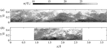
Example of instantaneous streamwise velocity fields. (a) Large field of view, (b) small field of view.

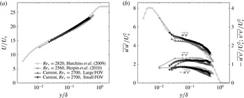
Boundary layer statistics. (a) Mean profile, (b) Reynolds stresses.

Two experiments were performed, one with a small FOV and one with a large FOV. Examples of velocity fields of both FOVs are shown in figure 1. To achieve the different magnifications the cameras were placed at about 40 cm and 90 cm from the measurement plane for the small FOV and large FOV, respectively. Each camera’s FOV was calibrated using a single calibration plate, which covered the complete combined FOV of all cameras and was aligned with the laser sheet.
Particle image pairs are captured and processed using LaVision software DaVis 7.2. Images were preprocessed using a min–max normalisation. Gaussian-weighted correlation started with an initial window size of
 $64\times 64$
pixels and finished at
 $16\times 16$
pixels with an overlap factor of 50 %. The resulting data of the large FOV covered an area of
 $37\times 4.6$
cm
 $^{2}$
(
 $3.7{\it\delta}\times 0.46{\it\delta}$
) with a spatial resolution of
 $h^{+}=22$
(
 $l^{+}=43$
) and a temporal resolution of
 ${\rm\Delta}t^{+}=1.5$
, and the small FOV covered an area of
 $17\times 4.5$
cm
 $^{2}$
(
 $1.7{\it\delta}\times 0.45{\it\delta}$
) with a spatial resolution of
 $h^{+}=10$
(
 $l^{+}=20$
) and a temporal resolution of
 ${\rm\Delta}t^{+}=0.7$
. A total of about 50 000 velocity fields were obtained for the small FOV – 10 runs of 5000 images over 5 s each – and 25 000 velocity fields for the large FOV – 5 runs of 5000 images over 10 s each – spanning a time interval of more than
 $300{\it\delta}/U$
.
The resulting boundary-layer mean velocity and Reynolds stresses agree with two previous studies at a comparable Reynolds number (figure 2: Hutchins et al. Reference Hutchins, Nickels, Marusic and Chong2009; Herpin, Stanislas & Soria Reference Herpin, Stanislas and Soria2010).
3. Frequency–wavenumber mapping
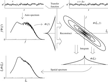
To map temporal spectra into spatial spectra, we move through the wavenumber–frequency plane, and the ideal mapping is the wavenumber–frequency spectrum itself. However, out of necessity, most approaches approximate this mapping function, and the shape of this plane depends on the approach taken. The complete mapping procedure consists of four steps. First, the temporal spectrum is determined; second, a transfer function – generally from two-point measurements – is obtained; third, the temporal spectrum is mapped onto the wavenumber–frequency plane using the transfer function; and last, the wavenumber–frequency spectrum is integrated across frequency to obtain the wavenumber spectrum. A schematic diagram of this process is depicted in figure 3.
Using a Taylor’s hypothesis mapping approach assumes the wavenumber–frequency spectrum to be a single line, creating unique wavenumber–frequency mapping pairs, which are related to one another by the phase velocity of each wave. In this case the process can be simplified into two steps: (1) determine the frequency spectrum and (2) map the frequencies to wavenumbers using the wave (convection) velocity. For wave velocities that are a function of frequency (and thus wavenumber), a non-uniform gain function has also to be applied in this second step. The main issue for Taylor’s hypothesis approaches is to find the correct convection velocity.
First we will look at what the wavenumber–frequency spectra should look like, and then we discuss the different convection (or wave) velocities.
Schematic of how to map a temporal spectrum into a spatial spectrum via the wavenumber–frequency plane for a single wall-normal location.

3.1. Wavenumber–frequency spectrum and wave velocities
Using our PIV data, we obtain spatial, temporal and wavenumber–frequency spectra (for a subdomain of the full range of scales) to see how they are related. The wavenumber–frequency spectrum at a given wall-normal location
 $y$
is the power spectral density
 ${\it\Phi}({\it\xi}_{x},f;y)$
as a function of wavenumber
 ${\it\xi}_{x}$
and frequency
 $f$
, where the wavenumber is the inverse of the wavelength
 ${\it\xi}_{x}=1/{\it\lambda}_{x}$
and the frequency the inverse of the waveperiod (time scale),
 $f=1/{\it\lambda}_{t}$
. The wavenumber and frequency are related to their angular counterparts by
 $k_{x}=2{\rm\pi}{\it\xi}_{x}$
and
 ${\it\omega}=2{\rm\pi}f$
.
Experimental data are limited in domain length and resolution. To minimise effects of truncation and account for differences in resolution, we determine the power spectral density by taking the following windowed and truncated two-dimensional Fourier transform of the velocity fluctuations:
 $$\begin{eqnarray}\hat{u} ({\it\xi}_{x},f;y)=\frac{1}{\displaystyle \sqrt{XT\int _{0}^{X}\int _{0}^{T}w(x,t)^{2}\,\text{d}t\,\text{d}x}}\int _{0}^{X}\int _{0}^{T}w(x,t)u^{\prime }(x,t;y)\text{e}^{-\text{i}2{\rm\pi}(ft+{\it\xi}_{x}x)}\,\text{d}t\,\text{d}x,\end{eqnarray}$$
where
 $X$
is the domain length,
 $T$
the sample time interval length and
 $w$
the weighting function (we used a Hamming window). Then the power spectral density is estimated as
 $$\begin{eqnarray}{\it\Phi}_{uu}({\it\xi}_{x},f;y)=\hat{u} ^{\ast }({\it\xi}_{x},f;y)\hat{u} ({\it\xi}_{x},f;y),\end{eqnarray}$$
where
 $\hat{u} ^{\ast }$
is the conjugate of
 $\hat{u}$
.
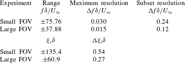
The frequency range and resolution as well as the wavenumber range and resolution that we can obtain from our PIV experiment are listed in table 1.
Nyquist range and resolution in the wavenumber–frequency plane based on time separation, sample length, interrogation window size and domain length.

3.1.1. Wavenumber–frequency spectrum
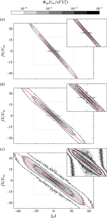
For each wall-normal location, the ideal mapping function is the wavenumber–frequency spectrum at that location, and this mapping function changes significantly with wall-normal location; see figure 4 for the frequency–wavenumber spectrum of the streamwise velocity at three different wall-normal locations. In our flow we have a positive velocity, which – due to the choice of transform – results in a negative slope (see figure 2 of Moin Reference Moin2009) of the distribution of the wavenumber–frequency spectrum. The main figure is the spectrum from the smaller FOV (and hence can reach higher frequencies and wavenumbers) while the data from the larger FOV are presented as an inset for all three locations. In the region where the two FOVs overlap, the results show good agreement, indicating that truncation effects do not significantly influence these results.
Wavenumber–frequency power spectral density of streamwise velocity fluctuations,
 ${\it\Phi}_{uu}$
, for three different wall-normal locations. The inset shows the same power spectral density obtained using the large FOV data. The diagonal red line (colour online, else grey line) indicates the local mean velocity. The extent (half the Nyquist range) of the spectral domain covered by the large FOV (inset) is indicated by the light grey box: (a)
 $y/{\it\delta}=0.46$
, (b)
 $y/{\it\delta}=0.010$
, (c)
 $y/{\it\delta}=0.026$
.

The width and symmetry of the spectra are a measure of the validity of Taylor’s hypothesis (McKeon & Sharma Reference McKeon and Sharma2010). The slope follows the local mean velocity and the spread of the contours decreases with increasing wall-normal location. This suggests that the range of convection velocities (and wave velocities) decreases with increasing wall-normal location (or decreasing turbulence intensities). Wall-normal velocity fluctuation spectra show similar behaviour and are not shown here for brevity.
3.1.2. Wave velocities
The main issue in Taylor’s hypothesis mapping approaches is to find the correct wave velocity. Wave velocities or phase velocities are velocities at which specific energy-containing waves,
 ${\it\Phi}({\it\xi}_{x},f;y)$
, travel and are given by
 $$\begin{eqnarray}u_{p}=-\frac{f}{{\it\xi}_{x}},\end{eqnarray}$$
where the minus sign is due to the choice of signs in the Fourier transform (3.1). Wave velocities differ from convection velocities (
 $u_{c}=-\langle \partial _{t}u\partial _{x}u\rangle /\langle (\partial _{x}u)^{2}\rangle$
, as defined by del Álamo & Jiménez Reference del Álamo and Jiménez2009) and they link a specific wavenumber to a specific frequency and can therefore be used to map the energy of a frequency to a wavenumber. However, due to the distribution of energy in the wavenumber–frequency plane, the energy of a single frequency will contribute to multiple wavenumbers. del Álamo & Jiménez (Reference del Álamo and Jiménez2009) show multiple ways to obtain – average – phase (wave) and convection velocities and state that the different velocities are not equivalent. The main reason for this is that wave velocity is only identical to the convection velocity if there is only one single wave or when all phase velocities are the same (Freegarde Reference Freegarde2013). When different waves have different phase velocities, their combined convection velocity will be different. It must be noted that use of Taylor’s hypothesis implies that all phase velocities are the same. Any deviation results in error, and therefore del Álamo & Jiménez (Reference del Álamo and Jiménez2009) introduce figures of merit for the frozen-turbulence assumption.
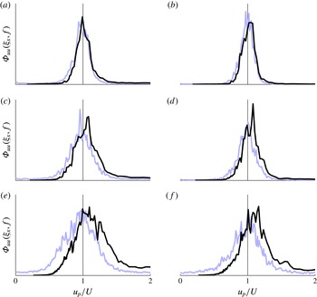
The difference between two ways of determining average wave velocities is the direction of integration (del Álamo & Jiménez Reference del Álamo and Jiménez2009). One can integrate over wavenumber direction – keeping frequency constant – or integrate over frequency direction – and keep wavenumber constant. For example, if we choose a constant frequency to examine wave velocities, we make cuts along wavenumber direction in the wavenumber–frequency spectra, and want to find the centre of gravity of the resulting distribution, but if we choose the wavenumber to be constant we take a cut in the frequency direction (see also Moin Reference Moin2009). Depending on the spread and shape of the wavenumber–frequency distribution, this results in different answers. To visualise this difference, figure 5 shows the two different cuts – expressed as a distribution of power spectral density with a wave velocity (using (3.3), see also Wills Reference Wills1964; Goldschmidt et al.
Reference Goldschmidt, Young and Ott1981) – for the same wall-normal locations as figure 4. A constant frequency is chosen for the small and large FOVs and constant wavenumbers are chosen such that the resulting cuts cross each other through the classic Taylor’s hypothesis point, i.e.
 ${\it\xi}_{x}=f/U\rightarrow u_{p}=U$
. The distributions differ significantly from each other near the wall, and with increasing wall-normal location they narrow and overlap more. This indicates that the spread of the wavenumber–frequency spectrum influences the difference between the two average wave velocities – each on one side of the local mean velocity.
Different ways of defining wave velocities can be applied to the power spectral energy distribution to obtain different wave velocities for each wall-normal location (similar to convection velocities from the correlation plane (see e.g. Wills Reference Wills1964; Goldschmidt et al.
Reference Goldschmidt, Young and Ott1981), velocities for which
 $\partial {\it\Phi}_{uu}/\partial {\it\xi}_{x}=0$
,
 $\partial {\it\Phi}_{uu}/\partial f=0$
or
 $\partial {\it\Phi}_{uu}/\partial u_{p}=0$
holds) and these definitions of wave velocity assume that a peak of the power (or energy) spectral density (in a direction) is the best representative of the overall phase velocity, in contrast with the weighted average of del Álamo & Jiménez (Reference del Álamo and Jiménez2009). For example, LeHew et al. (Reference LeHew, Guala and McKeon2011) trace the ridge of a premultiplied spectrum. However – as also observed in earlier studies – the actual spectra show a distribution around this peak or average (figure 5), which means that a single wave velocity will not capture the transfer function correctly. The main issue is that the power of one frequency contributes to the power of multiple wavenumbers and vice versa. Farther away from the wall (
 $y/{\it\delta}\approx 0.46$
), the two power distributions with wave velocity appears similar, symmetric and with a small spread, suggesting that the effect of the distribution on wave velocities will be small. In contrast, closer to the wall (
 $y/{\it\delta}=0.026$
), the distribution is wider and shows an asymmetry that will have an influence on mapping frequency to wavenumber and vice versa.
Power spectral density distributions with wave velocity,
 $u_{p}=-f/{\it\xi}_{x}$
. Spread of power spectral density along cuts – with constant frequency or wavenumber (black or blue line respectively, colour online, else black or grey line) – of the wavenumber–frequency spectra in figure 4. The cuts are chosen such that they each pass through the Taylor’s hypothesis mapping point,
 ${\it\xi}_{x}=f/U\rightarrow u_{p}=U$
, indicated by the vertical line. (a,c,e) Small FOV
 $f{\it\delta}/U_{\infty }=21$
(black line);
 ${\it\xi}_{x}{\it\delta}=23$
(a), 29 (c), 36 (e) (blue lines). (b,d,f) Large FOV
 $f{\it\delta}/U_{\infty }=10$
(black line);
 ${\it\xi}_{x}{\it\delta}=11$
(b), 14 (d), 16 (f) (blue lines). (a,b)
 $y/{\it\delta}=0.46$
; (c,d)
 $y/{\it\delta}=0.10$
; (e,f)
 $y/{\it\delta}=0.026$
.

del Álamo & Jiménez (Reference del Álamo and Jiménez2009) propose a semi-empirical approach that uses a convolution window that acts on the mean velocity and results in a wavenumber-dependent convection velocity and gain function, which acts as a reduced model of the full wavenumber–frequency spectrum. To account for the spread in wave velocities this convolution window depends on wavelength (in streamwise and spanwise directions) and wall-normal distance. This convolution window needs to be estimated from numerical or experimental data and ideally should cover a wide range of Reynolds numbers. This requires more than the commonly applied two-point measurements and is difficult to use – at least until a good (model) convolution window is determined. Moreover, as they state, this approach is valid only for channel flow (or perhaps even pipes) while its applicability in boundary layers or other types of shear flows remains unresolved.
3.2. Frequency–wavenumber mapping using a cross-spectral approach
To bypass the issues with finding an appropriate approximation of the wavenumber–frequency plane, we propose to reconstruct the wavenumber–frequency plane (the ideal mapping function) by using a two-point cross-spectral approach based on distributions of cross-spectral phase difference – equivalent to distributions of wave velocity. The resulting transfer function can differ from flow to flow and location to location and our approach will capture the transfer function for the flow and location to which it is applied. Therefore, it provides a data-driven methodology that can be applied to any turbulent flow at any location. Integrating the resulting wavenumber–frequency spectrum in the frequency direction leads to the wavenumber spectrum. So, to map temporal spectra into spatial spectra we move through the wavenumber–frequency plane, and rather than simplifying this plane to a single line (as is done by Taylor’s hypothesis and approaches based on it), our approach reconstructs the full wavenumber–frequency plane.
To map the frequency spectrum into a wavenumber spectrum (at a single wall-normal location), we follow four steps, as outlined in figure 3: (i) determine the auto-spectrum from single-point measurement, (ii) determine a transfer function using cross-spectra of two-point measurements, (iii) reconstruct the wavenumber–frequency spectrum by applying the transfer function to the auto-spectrum, and, finally, (iv) integrate the wavenumber–frequency spectrum to obtain the spatial spectrum.
First, we start with the one-dimensional truncated weighted Fourier transform (to avoid any influences of our limited PIV domain),
 $$\begin{eqnarray}\hat{u} _{x}(\,f;x,y)=\frac{1}{\displaystyle \sqrt{T\int _{0}^{T}w(t)^{2}\,\text{d}t}}\int _{0}^{T}w(t)u^{\prime }(t;x,y)\text{e}^{-\text{i}2{\rm\pi}ft}\,\text{d}t\end{eqnarray}$$
from which the auto-spectral power density,
 ${\it\Phi}_{x}$
, as a function of frequency can be determined:
 $$\begin{eqnarray}{\it\Phi}_{x}(f;x,y)=\hat{u} _{x}^{\ast }(f;x,y)\hat{u} _{x}(f;x,y).\end{eqnarray}$$
This gives us the frequency spectrum as a function of wall-normal (and streamwise) location. We take multiple spectra and average them to get a converged frequency spectrum, as is common in determining turbulence spectra.
Then, the cross-spectrum between two different spatial locations separated by
 ${\rm\Delta}x$
is determined:
 $$\begin{eqnarray}{\it\Psi}_{x}(f;x,{\rm\Delta}x,y)=\hat{u} _{x}^{\ast }(f;x,y)\hat{u} _{x}(f;x+{\rm\Delta}x,y),\end{eqnarray}$$
from which the cross-spectral power density,
 $|{\it\Psi}_{x}|$
, and the phase spectrum,
 ${\it\psi}_{x}$
, are obtained:
 $$\begin{eqnarray}{\it\psi}_{x}(f;x,{\rm\Delta}x,y)=\tan ^{-1}\frac{\text{Im}({\it\Psi}_{x})}{\text{Re}({\it\Psi}_{x})}.\end{eqnarray}$$
The resulting phase shift is used to estimate the corresponding wavenumber,
 $\tilde{{\it\xi}}_{x}$
,
 $$\begin{eqnarray}\tilde{{\it\xi}}_{x}(f;x,{\rm\Delta}x,y)=\frac{{\it\psi}_{x}(f;x,{\rm\Delta}x,y)}{2{\rm\pi}{\rm\Delta}x}.\end{eqnarray}$$
Each cross-spectrum is a unique frequency–wavenumber mapping, having a single phase velocity for each frequency (and, therefore, wavenumber).
Cenedese et al. (Reference Cenedese, Romano and Di Felice1991) and Romano (Reference Romano1995) used the average of these phase velocities to determine frequency-dependent convection velocities, similar to the (weighted) average phase velocity as given by del Álamo & Jiménez (Reference del Álamo and Jiménez2009). Averaging increases the accuracy of the (average) phase change, but it also removes the spread present in phase velocities and is susceptible to spectral folding. This spectral folding results in a decrease in coherence (modulus of transfer function in figure 10 of Cenedese et al. (Reference Cenedese, Romano and Di Felice1991)) and the wrong average phase velocity (possibly the explanation for the abrupt change in average phase velocity for the larger separation distances in figure 11 of Cenedese et al. (Reference Cenedese, Romano and Di Felice1991)). If the phase difference for a specific frequency is determined within a range from
 $-{\rm\pi}$
to
 ${\rm\pi}$
, then the energy present in phase differences just larger than
 ${\rm\pi}$
will be folded back into this range, just above
 $-{\rm\pi}$
, resulting in a wrong average phase difference.
To regain the distribution of phase velocities that is present in the wavenumber–frequency spectrum, we use multiple cross-spectra to create probability density functions of phase difference per frequency – weighted with cross-spectral energy – and with these form the basis of the transfer function
 $G(x,\tilde{{\it\xi}}_{x},{\rm\Delta}x,f,y)$
. To mitigate the effect of spectral folding we apply an unfolding technique (see Buxton et al.
Reference Buxton, de Kat and Ganapathisubramani2013), where we shift the range of phases to be around the average phase shift that the local mean velocity will give for that frequency. This resembles the way the wavenumber–frequency spectrum appears to be spread around the local mean velocity.
The wavenumber–frequency spectrum is then obtained by multiplying the transfer function by the auto-spectral power density,
 $$\begin{eqnarray}\tilde{{\it\Phi}}(\tilde{{\it\xi}}_{x},f;x,{\rm\Delta}x,y)={\it\Phi}(f;x,y)G(\tilde{{\it\xi}}_{x},f;x,{\rm\Delta}x,y),\end{eqnarray}$$
and, finally, integration over frequency direction results in the spatial spectrum:
 $$\begin{eqnarray}\tilde{{\it\Phi}}(\tilde{{\it\xi}}_{x};x,{\rm\Delta}x,y)=\int \tilde{{\it\Phi}}(\tilde{{\it\xi}}_{x},f;x,{\rm\Delta}x,y)\,\text{d}f.\end{eqnarray}$$
This approach can also be used to determine the mapping of the spatial spectrum into the temporal spectrum – to map direct numerical simulation (DNS) results into frequency spectra for comparison with experiments – by starting from two spatial signals at two different time instances and following the same procedure, replacing
 $x$
by
 $t$
,
 $f$
by
 ${\it\xi}_{x}$
and
 $\tilde{{\it\xi}}_{x}$
by
 $\tilde{f}$
.
3.3. Reconstructed wavenumber–frequency and mapped spectra
Using our turbulent boundary layer data, we reconstruct the wavenumber–frequency spectra over the same range of wavenumbers and frequencies for which we have the direct information, as in figure 4. We then integrate these to obtain spatial spectra, which we compare with direct spatial spectra and the spectrum obtained by using Taylor’s hypothesis.
3.3.1. Reconstructed wavenumber–frequency spectra
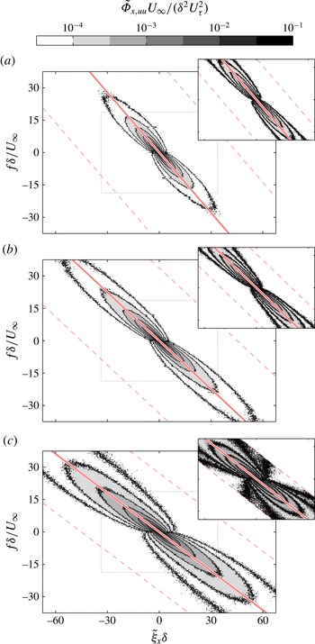
The resulting wavenumber–frequency spectra for the streamwise velocity fluctuations, figure 6, are largely similar to the direct wavenumber–frequency spectra, but with two main differences.
Reconstructed wavenumber–frequency power spectral density of streamwise velocity fluctuations,
 $\tilde{{\it\Phi}}_{x,uu}$
, for three different wall-normal locations. The diagonal red line (colour online, else grey line) indicates the local mean velocity, the diagonal dashed red lines (colour online, else dashed grey lines) indicate the area within
 $\pm {\rm\pi}$
from the local mean velocity that is used for the reconstruction, and the extent (half the Nyquist range) of the spectral domain covered by the large FOV (inset) is indicated by the light grey box. Measurement point separation is
 ${\rm\Delta}x/{\it\delta}=0.011$
and
 ${\rm\Delta}x/{\it\delta}=0.025$
for the small FOV and large FOV respectively: (a)
 $y/{\it\delta}=0.46$
, (b)
 $y/{\it\delta}=0.010$
, (c)
 $y/{\it\delta}=0.026$
.

First, near
 $f=0$
the distribution shows a kink, rather than a continuous behaviour as in figure 4. This is an effect of limited sample length, indicating insufficient frequency resolution. The results from the large FOV show this effect to a lesser extent, due to their longer sample length; see the inset in figure 4. This effect can be corrected (see Buxton et al.
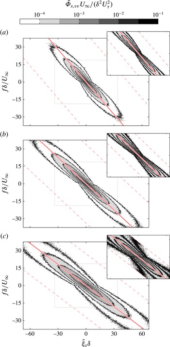
Reference Buxton, de Kat and Ganapathisubramani2013); however, it is best to obtain a longer time signal to overcome this problem. Performing the mapping for wall-normal velocity fluctuations, where most of the relevant temporal scales are captured, reduces the truncation effect, as shown in figure 7. This indicates that if one captures all flow scales, there are no issues due to truncation in reconstructing the wavenumber–frequency spectrum.
Second, the distribution in the reconstructed wavenumber–frequency spectra in figure 6 is more spread out than the direct spectra in figure 4, and wall-normal velocity fluctuations in figure 7 show a similar difference to their reference (the latter not shown for brevity). This additional spread is due to measurement noise (Buxton et al.
Reference Buxton, de Kat and Ganapathisubramani2013) and can be reduced if the spatial separation is increased. However, increasing
 ${\rm\Delta}x$
reduces the frequency range that can be captured – see the Appendix – and also increases the influence of shear (Davies & Fisher Reference Davies and Fisher1963). Therefore, the spatial separation
 ${\rm\Delta}x$
should be chosen to balance the effect of measurement noise with that of the desired frequency range. A comparison between the small FOV results and the large FOV results in figures 6 and 7 shows that the spread is indeed reduced for a larger separation distance, but the reconstruction range is reduced; see the Appendix.
Reconstructed wavenumber–frequency power spectral density of wall-normal velocity fluctuations,
 $\tilde{{\it\Phi}}_{x,vv}$
, for three different wall-normal locations. The diagonal red line (colour online, else grey line) indicates the local mean velocity, the diagonal dashed red lines (colour online, else dashed grey lines) indicate the area within
 $\pm {\rm\pi}$
from the local mean velocity that is used for the reconstruction, and the extent (half the Nyquist range) of the spectral domain covered by the large FOV (inset) is indicated by the light grey box. Measurement point separation is
 ${\rm\Delta}x/{\it\delta}=0.011$
and
 ${\rm\Delta}x/{\it\delta}=0.025$
for the small FOV and large FOV respectively: (a)
 $y/{\it\delta}=0.46$
, (b)
 $y/{\it\delta}=0.010$
, (c)
 $y/{\it\delta}=0.026$
.

It is important to stress that both above-mentioned differences are unique to PIV data (due to dynamic range issues) and are likely to reduce when applying the approach to two-point hot-wire data, since hot-wire measurements allow for longer time series and have lower measurement noise.
3.3.2. Temporal spectra mapped into spatial spectra
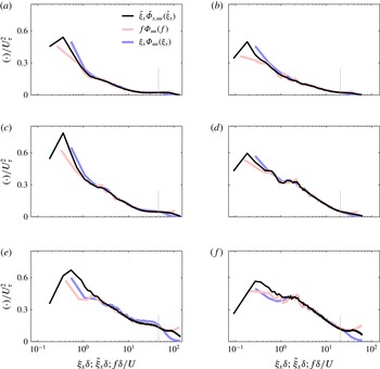
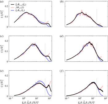
Now we can determine the wavenumber spectra using the reconstructed wavenumber–frequency spectra of figures 6 and 7 by integrating along the frequency axis and compare them to the direct spatial spectrum and classic Taylor’s hypothesis mapping.
Mapped and original streamwise velocity fluctuation spectra for three different wall-normal locations. Direct spatial spectrum (blue line, colour online, else dark grey line), Taylor’s hypothesis mapping (red line, colour online, else light grey line) and current mapping (black line). Vertical grey lines indicate the inverse of separation distance. Measurement point separation is
 ${\rm\Delta}x/{\it\delta}=0.011$
and
 ${\rm\Delta}x/{\it\delta}=0.025$
for the small FOV (a,c,e) and large FOV (b,d,f) respectively; (a,b)
 $y/{\it\delta}=0.46$
, (c,d)
 $y/{\it\delta}=0.010$
, (e,f)
 $y/{\it\delta}=0.026$
.

Mapped and original wall-normal velocity fluctuation spectra for three different wall-normal locations. Direct spatial spectrum (blue line, colour online, else dark grey line), Taylor’s hypothesis mapping (red line, colour online, else light grey line) and current mapping (black line). Vertical grey lines indicate the inverse of separation distance. Measurement point separation is
 ${\rm\Delta}x/{\it\delta}=0.011$
and
 ${\rm\Delta}x/{\it\delta}=0.025$
for the small FOV (a,c,e) and large FOV (b,d,f) respectively; (a,b)
 $y/{\it\delta}=0.46$
, (c,d)
 $y/{\it\delta}=0.010$
, (e,f)
 $y/{\it\delta}=0.026$
.

Comparison of all three spectra – direct, Taylor’s hypothesis mapped and current mapping approach spectra – for the streamwise velocity fluctuations at different wall-normal locations shows a remarkable agreement for the captured scales, see figure 8. Except for the truncated lower wavenumbers, both the Taylor’s hypothesis mapping and our cross-spectral approach mapping lie on top of the spatial spectrum. Compared with the effect that the spatial separation
 ${\rm\Delta}x$
has on the reconstructed wavenumber–frequency spectrum, its effect on the mapping is limited, see the Appendix. The spatial spectra for the wall-normal velocity fluctuations, in figure 9, show that the lower wavenumbers will also be mapped correctly if they are captured sufficiently in the temporal spectrum.
This agreement between our approach and the direct spatial spectra shows that our reconstruction of the wavenumber–frequency spectra works, and we can use it to map frequency spectra into wavenumber spectra, provided that we have sufficiently long temporal data to obtain the entire range of wavenumber spectra.
4. Discussion
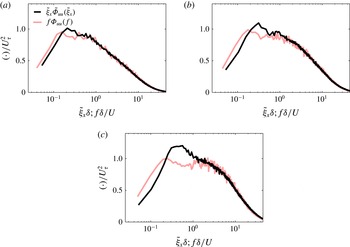
The comparison between three different wavenumber spectra (direct, our mapping and Taylor’s hypothesis) in the previous section shows that Taylor’s hypothesis is applicable for large wavenumbers (small scales), which agrees with Lin (Reference Lin1953), and the cross-spectral approach gives similar results. However, the more pertinent question is what happens at the smaller wavenumbers (large scales), where differences are expected (Lin Reference Lin1953; del Álamo & Jiménez Reference del Álamo and Jiménez2009). Our PIV data for a turbulent boundary layer are not sufficiently long (in time and space) to make this comparison directly. Therefore, we use the time series of our PIV data to obtain the transfer function for a range of wall-normal locations, apply this transfer function to frequency spectra from hot-wire data at a comparable Reynolds number, and use the resulting reconstructed wavenumber–frequency plane to map the hot-wire frequency spectra into wavenumber spectra.
We use the PIV data to determine the transfer function over the largest possible range of frequencies (see table 1) from our spatially best resolved measurement, the small FOV. We obtain transfer functions from our data for 36 wall-normal locations within our small FOV – spaced logarithmically in wall-normal direction to match the hot-wire spacing. This transfer function is then applied to hot-wire data at a comparable Reynolds number (data from Hutchins et al. Reference Hutchins, Nickels, Marusic and Chong2009). The transfer function closest to each hot-wire wall-normal location is used and is corrected for the (small) difference in local mean velocity. Integration of the resulting reconstructed wavenumber–frequency plane completes the mapping of the frequency spectra into wavenumber spectra.
Premultiplied mapped power density spectra of hot-wire data at a Reynolds number
 $Re_{{\it\tau}}=2820$
from Hutchins et al. (Reference Hutchins, Nickels, Marusic and Chong2009) using Taylor’s hypothesis (red line colour online, else grey line) and our mapping (black line) for three different wall-normal locations: (a)
 $y/{\it\delta}=0.111$
,
 $y^{+}=314$
; (b)
 $y/{\it\delta}=0.055$
,
 $y^{+}=154$
; (c)
 $y/{\it\delta}=0.027$
,
 $y^{+}=76$
.

Mapped spectra for three different wall-normal locations are shown in figure 10. As expected, Taylor’s hypothesis mapping and our proposed mapping give similar results for large wavenumbers (small scales). In contrast, the difference for lower wavenumbers (large scales) is significant and the double-peaked spread that is present for Taylor’s hypothesis (figure 10) is contracted in the cross-spectral approach. The resulting difference in the power density for
 $y^{+}=76$
is over
 $+30$
% for
 $0.45<{\it\xi}_{x}{\it\delta}<0.67$
and
 $-30$
% for
 ${\it\xi}_{x}{\it\delta}<0.1$
.
The (non-)existence of the double peak in the spectra is consistent with the result of del Álamo & Jiménez (Reference del Álamo and Jiménez2009), who noted that the double peak disappears when they applied their convection-velocity mapping to experimental data obtained in pipe flows. This suggests that the mapping proposed in the current study is as effective as the convolution window based mapping presented in del Álamo & Jiménez (Reference del Álamo and Jiménez2009). The difference between the two approaches is that our frequency–wavenumber mapping is a data-driven approach that relies on simultaneous two-point measurements that can be easily obtained via hot-wire experiments. In fact, most studies in the literature use two-point measurements to determine convection velocities (Harrison Reference Harrison1958; Davies & Fisher Reference Davies and Fisher1963; Davies et al. Reference Davies, Fisher and Barrat1963; Fisher & Davies Reference Fisher and Davies1964; Wills Reference Wills1964; Goldschmidt et al. Reference Goldschmidt, Young and Ott1981; Cenedese et al. Reference Cenedese, Romano and Di Felice1991; Romano Reference Romano1995; Krogstad et al. Reference Krogstad, Kaspersen and Rimestad1998).
The difference in spectra from Taylor’s hypothesis and from our mapping is consistent with recent findings based on instantaneous structure tracking. For example, Lee et al. (Reference Lee, Lee, Choi and Sung2014) found that regions of large positive streamwise velocity fluctuation move faster than the average velocity and regions of large negative streamwise velocity fluctuation move slower than the average velocity. We have made similar observations by tracking individual structures in space and time in our time-resolved PIV data (de Kat & Ganapathisubramani Reference de Kat and Ganapathisubramani2014). This means that positive and negative streamwise velocity fluctuation regions of the same size can give rise to different frequencies (de Kat & Ganapathisubramani Reference de Kat and Ganapathisubramani2013). This would explain the double peak in the frequency spectra, since this behaviour results in a bimodal distribution – similar to the probability function of a sinusoidal wave (with some added noise). However, mapping via the reconstructed wavenumber–frequency spectrum – including the spread of phase velocities – turns the double peak in the frequency spectrum back into a single peak in the wavenumber spectrum.
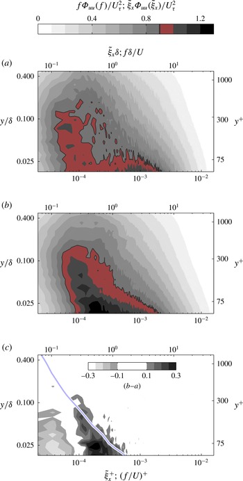
If we now take a global view and look at wavenumber spectra for a range of wall-normal locations at the same time in a spectrograph (contour plot) of power spectral density, shown in figure 11, we can see the differences between using Taylor’s hypothesis (figure 11
a) and our mapping approach (figure 11
b). For the Taylor’s hypothesis mapping, we can clearly see two regions: one small-wavenumber region (
 ${\it\xi}_{x}{\it\delta}\approx 0.16$
;
 ${\it\lambda}_{x}/{\it\delta}\approx 6$
) that corresponds to the outer region and has a clear presence below
 $y/{\it\delta}<0.1$
in figure 11(a), and the top of the inner region at
 ${\it\xi}_{x}^{+}\approx 10^{-3}$
(
 ${\it\lambda}_{x}^{+}\approx 1000$
) at the lowest wall-normal location that we can map.
In a theoretical exposition, Lin (Reference Lin1953) showed that Taylor’s hypothesis will only hold for wavenumbers that satisfy
 $kU\gg \text{d}U/\text{d}y$
, and if we look at the difference between the Taylor’s hypothesis and our current mapping, figure 11(c), we see that changes are primarily located in the range
 $kU<\text{d}U/\text{d}y$
, supporting Lin’s prediction on where Taylor’s hypothesis holds and where it fails. The range of wall-normal locations where we see a significant change is restricted to
 $y/{\it\delta}<0.1$
, where the ratio of fluctuating to local mean velocity ratio is significant as well (
 $\sqrt{u^{\prime 2}}/U$
above 10 %).
Premultiplied mapped power density spectra of hot-wire data at a Reynolds number
 $Re_{{\it\tau}}=2820$
from Hutchins et al. (Reference Hutchins, Nickels, Marusic and Chong2009) with wall-normal location,
 $y/{\it\delta}$
. (a) Classic Taylor’s hypothesis mapping using the local mean velocity. (b) Current mapping based on cross-spectra. (a,b) To facilitate comparison, one level is outlined and shaded red (colour online, else only outlined). (c) Difference between our current mapping and Taylor’s hypothesis mapping. The blue line (colour online, else grey line) demarcates the wavenumber limit predicted by Lin (Reference Lin1953),
 $kU=\text{d}U/\text{d}y$
.

The inner and outer regions present in spectra obtained by Taylor’s hypothesis mapping are clearly described by Hutchins & Marusic (Reference Hutchins and Marusic2007) and they are exploited by Mathis, Hutchins & Marusic (Reference Mathis, Hutchins and Marusic2011) to model the inner–outer relation of streamwise velocity fluctuations in wall-bounded flows. However, if we now look at our cross-spectral mapping result in figure 11(
 $b$
), we see that the distinction between these regions has disappeared. The low-wavenumber ridge (large wavelengths) has moved higher and tilted (i.e. moved more at lower wall-normal distances) and at the same time the top of the inner region has moved to lower wavenumber (larger wavelengths) and merged with the ridge of the low wavenumbers that moved to higher wavenumbers. Instead of two distinct regions, we now see a single ridge, which connects the top of the inner region with the outer region.
For a higher Reynolds number, Rosenberg et al. (Reference Rosenberg, Hultmark, Vallikivi, Bailey and Smits2013) find that the double peak in wavenumber space still exists in their data even when they use the mapping from del Álamo & Jiménez (Reference del Álamo and Jiménez2009), in contrast with what del Álamo & Jiménez (Reference del Álamo and Jiménez2009) find for their lower Reynolds number. In fact, Rosenberg et al. (Reference Rosenberg, Hultmark, Vallikivi, Bailey and Smits2013) obtained their wavenumber spectra by extrapolating the model from del Álamo & Jiménez (Reference del Álamo and Jiménez2009) to a Reynolds number that is over an order of magnitude larger. This is very interesting in light of other efforts aimed at locating a
 $k_{x}^{-1}$
-region in the spectra using hot-wire data and Taylor’s hypothesis.
Perry & Abell (Reference Perry and Abell1975) state there should exist an overlap region between the inner and outer regions and this overlap should manifest itself as a
 $k_{x}^{-1}$
-region in the premultiplied wavenumber spectrum. They show the existence of such a region in turbulent pipe flow data. Nickels et al. (Reference Nickels, Marusic, Hafez and Chong2005) hint at the existence of this
 $k_{x}^{-1}$
-region in turbulent boundary layers, but its extent is very limited. To our knowledge, there is very little experimental evidence for the existence of this region over a large wavenumber range. This could be due to a lack of scale separation in the measurements. However, even pipe and boundary layer data for very high Reynolds numbers from the Princeton superpipe and HRTF (Vallikivi, Ganapathisubramani & Smits Reference Vallikivi, Ganapathisubramani and Smits2015) do not conclusively show the presence of this
 $k_{x}^{-1}$
-region. Therefore, the lack of
 $k_{x}^{-1}$
-region could be due to our limitation in determining the appropriate transfer function for these flows.
For increasing Reynolds numbers, Perry & Abell (Reference Perry and Abell1975) hypothesise that the fractional spread of phase velocities could reduce. Even over the ‘low’-Reynolds-number range examined in del Álamo & Jiménez (Reference del Álamo and Jiménez2009), convection velocity does indeed depend on the Reynolds number. This dependence of phase velocities on Reynolds number can convert a premultiplied wavenumber spectrum with a plateau (a pure
 $k_{x}^{-1}$
-region) into a double-peaked frequency spectrum. In fact, the wavenumber spectrum could even retain the double peak – with a
 $k_{x}^{-1}$
-region in between. Very recent DNS of a channel at
 $Re_{{\it\tau}}\approx 5200$
by Lee & Moser (Reference Lee and Moser2015) appear to support the latter statement as their data show a double peak in the premultiplied wavenumber spectrum with a
 $k_{x}^{-1}$
-region between the peaks. However, as the authors say in their paper, the development of the double peak and the plateau region with increasing Reynolds number remains an open question. Our cross-spectral mapping approach on two-point measurements – which can be applied to any flow – lays the foundation to tackle this open question.
5. Conclusion
To aid the correct mapping of temporal turbulence spectra into spatial spectra, we have proposed a two-point cross-spectral approach that uses a distribution of cross-spectral phase differences – equivalent to a distribution of wave velocities – to reconstruct the entire wavenumber–frequency plane. This plane can then be integrated to obtain the spatial or temporal spectrum depending on the input data. Since the technique is a purely data-driven approach, it can be employed in other shear flows as well as in wall-bounded flows at higher Reynolds numbers in order to examine the energy content in spatial scales without invoking Taylor’s hypothesis.
The new technique was verified on time-resolved PIV data from a turbulent boundary layer. Transfer functions for a range of wall-normal locations were obtained from this data set and these transfer functions were applied to hot-wire data at a comparable Reynolds number. Comparison of the newly proposed technique with the classical Taylor’s hypothesis approach shows that Taylor’s hypothesis holds for larger wavenumbers (small spatial scales). However, for smaller wavenumbers (large spatial scales) there are significant differences, which have implications for potential double-peaked turbulence spectra and possible
 $k_{x}^{-1}$
-regions.
Acknowledgements
We gratefully acknowledge the support from UK Engineering and Physical Sciences Research Council (EPSRC) through Grant EP/I004785/1 and the European Research Council under the European Union’s Seventh Framework Programme (FP7/2007-2013)/ERC Grant agreement no 277472-WBT. The authors would like to thank Drs L. Gan and J. Dawson for their hospitality during the visit of R.deK. to Cambridge University Engineering Department. The authors also thank Dr N. Hutchins for making his hot-wire data available. The authors would like to thank the reviewers for their critical comments and supportive suggestions. Finally, the authors are grateful to Dr T. Nickels for the inspiration for this work and the use of his water tunnel. Unfortunately, he passed away before the work in this project started.
Influence of spatial separation distance
 ${\rm\Delta}x$
on reconstructed wavenumber–frequency power spectral density of streamwise velocity fluctuations,
 $\tilde{{\it\Phi}}_{x,uu}$
, for three different wall-normal locations. For comparison direct wavenumber–frequency spectra (from figure 4) are shown on top. The diagonal red line (colour online, else grey line) indicates the local mean velocity; the diagonal dashed red lines (colour online, else dashed grey lines) indicate the area within
 $\pm {\rm\pi}$
from the local mean velocity that is used for the reconstruction.

Influence of separation distance
 ${\rm\Delta}x$
on mapped and original streamwise velocity fluctuation spectra for three different wall-normal locations. Direct spatial spectrum (blue line, colour online, else dark grey line), Taylor’s hypothesis mapping (red line, colour online, else light grey line) and current mapping (black line). Vertical grey lines indicate the inverse of separation distance.

Influence of spatial separation distance
 ${\rm\Delta}x$
on mapped and original wall-normal velocity fluctuation spectra for three different wall-normal locations. Direct spatial spectrum (blue line, colour online, else dark grey line), Taylor’s hypothesis mapping (red line, colour online, else light grey line) and current mapping black line. Vertical grey lines indicate the inverse of separation distance.

Appendix. Influence of spatial separation distance – and measurement noise – on the reconstruction of wavenumber–frequency spectra and the quality of the frequency–wavenumber mapping
To test the influence of the separation distance, we reconstructed wavenumber–frequency spectra for five different separation distances, shown in figure 12, starting from the smallest
 ${\rm\Delta}x/{\it\delta}=0.004$
to five times larger
 ${\rm\Delta}x/{\it\delta}=0.018$
, at the same wall-normal locations as in figures 4 and 6. The spread decreases with increasing separation distance. This effect is expected, since for larger displacements the influence of the (fixed) noise in the measurement system has a smaller (relative) influence.
However, due to the reconstruction technique the range of frequencies and wavenumbers becomes more and more restricted. The larger the separation distance, the smaller the bandwidth of the reconstructed wavenumber–frequency spectrum.
The effect of the spatial separation distance on the frequency–wavenumber mapping is also considered, and figures 13 and 14 show the result of the frequency–wavenumber mapping for different separation distances compared with spectra using Taylor’s hypothesis and direct spatial spectra. For both streamwise velocity fluctuation spectra (figure 13) and the wall-normal velocity fluctuation spectra (figure 14) the frequency–wavenumber spectra using the current mapping show good agreement for
 ${\rm\Delta}x/{\it\delta}>0.01$
, but for
 ${\rm\Delta}x/{\it\delta}<0.01$
the spreading of the reconstructed wavenumber–frequency spectra appears to result in an upward shift of the wavenumber spectrum using the current approach.
The two effects that the separation distance has are a noise effect for small
 ${\rm\Delta}x$
and a too narrow bandwidth restricting deviations from the classic Taylor’s hypothesis for large
 ${\rm\Delta}x$
. To balance the influence of these effects, we chose to use
 ${\rm\Delta}x/{\it\delta}=0.011$
for the small field of view in our current study.