





Introduction
Wild blueberries (Vaccinium angustifolium Aiton) are rhizomatous woody perennials in the family Ericaceae that is native to eastern North America with commercial industries in eastern Canada and Maine, USA. These plants are “wild” because they are not bred or planted, with populations occurring naturally on mountain tops and forests (Jensen and Yarborough Reference Jensen and Yarborough2004). In Maine, the wild blueberry crop is one of the top three specialty crops of the state, having a 5-yr average production (2020–2024) of 4,409 kg ha−1 (USDA-NASS 2024). Commercial fields of wild blueberry in Maine consist of natural stands managed using modern farming practices for maximum production (Yarborough Reference Yarborough2012) with a total harvested hectarage of approximately 7,900 ha (USDA-NASS 2024). Wild blueberries follow a 2-yr production cycle; the prune year and the crop year. The prune year is when wild blueberry plants are pruned by flail mowing or burning to stimulate new vegetative growth and bud development, followed by a crop year when blueberry plants flower and produce fruit. This 2-yr production cycle reduces pest problems and encourages wild blueberries to grow vigorously and maintain their yield over the long term (Yarborough Reference Yarborough2015).
Broadleaf and grass weeds are a significant challenge in wild blueberry production, causing yield losses through competition for water, light, nutrients, and space (Jensen and Yarborough Reference Jensen and Yarborough2004). Their random distribution and perennial growth, including rhizomatic habits similar to wild blueberry, make them difficult to manage (Wu et al. Reference Wu, Boyd, Cutler and Olson2013). Current integrated weed management (IWM) practices include mechanical, cultural, biological, and chemical methods (Kudsk Reference Kudsk2022), but mechanical approaches can be ineffective or costly at large scales, while cultural practices alone provide insufficient control (Baccin and Moretti Reference Baccin and Moretti2025; Calderwood Reference Calderwood2023; Landefeld et al. Reference Landefeld, Penrose, McCutcheon and Wiseman2017; Yarborough and Calderwood Reference Yarborough and Calderwood2020). Herbicides remain the most reliable and cost-effective option but are typically applied uniformly across entire fields despite weeds occurring only in patches. Broadcast applications therefore increase unnecessary herbicide use and the risk of environmental contamination through drift, leaching, runoff, and erosion, while also increasing selection pressure for herbicide resistance (Cederlund Reference Cederlund2017; Upadhyay et al. Reference Upadhyay, Sunil, Yu, Koparan and Sun2024; White Reference White2019; Yarborough Reference Yarborough2002; Zaman et al. Reference Zaman, Schumann and Percival2010). Targeted herbicide application is thus needed to reduce chemical inputs while maintaining effective weed control. Drones, or uncrewed aerial vehicles (UAVs), can support site-specific weed management (SSWM) by enabling precise mapping and treatment of weed infestations, providing an additional tool within the IWM framework (Hunter et al. Reference Hunter, Gannon, Richardson, Yelverton and Leon2020).
Targeted weed control first requires accurate identification and spatial mapping of weed infestations within fields (Nobre et al. Reference Nobre, Santos, Herrera, Araújo, Johann, Gurgacz, Siqueira and Prior2023). Under SSWM, drones equipped with red–green–blue (RGB), multispectral, or hyperspectral sensors, are used to generate drone aerial images or orthomosaics (Esposito et al. Reference Esposito, Crimaldi, Cirillo, Sarghini and Maggio2021). These orthomosaics result in weed maps that differentiate between weeds and non-weeds (López-Granados et al. Reference López-Granados, Torres-Sánchez, Serrano-Pérez, De Castro, Mesas-Carrascosa and Peña-Barragán2016) or between and among weed species (Sandino and Gonzales Reference Sandino and Gonzalez2018; Tiwari et al. Reference Tiwari, Goyal, Kumar and Vij2019). Weed mapping in wild blueberry fields can easily be made due to the contrast of colors between weeds and wild blueberry plants (Bilodeau et al. Reference Bilodeau, Esau, MacEachern, Farooque, White and Zaman2023). During the early prune year, or the time before wild blueberry plants start to vegetate, wild blueberry plants are reddish brown while weeds are light brown/green in color. Early prune year weeds, often light brown in color, are dried remains from the previous year’s growth. With conditions favorable for germination, new leaves emerge from these dried remains or directly from the ground, creating a combination of colors contrasting with the reddish-brown colors of pruned wild blueberry plants (Figure 1). These color contrasts between weeds and wild blueberry plants during the early prune year enable their differentiation using RGB drone imagery, as RGB sensors capture reflectance within the visible portion of the electromagnetic spectrum.
Weed patches (white and green colors) and wild blueberry (dark brown and red) in mid-April (left) and late May (right) in Harrington, ME.

Recent studies on weed mapping in wild blueberry fields have conducted image analysis using ground and drone imagery. Hennessy et al. (Reference Hennessy, Esau, Farooque, Schumann, Zaman and Corscadden2021) explored deep learning convolutional neural networks to identify hair fescue (Festuca filiformis Pourr.) and sheep sorrel (Rumex acetosella L.) in wild blueberry fields using a handheld digital camera. Their study resulted in high weed detection F1 scores of 0.97 and 0.96 for F. filiformis and 0.90 and 0.95 for R. acetosella using the YOLOv3-Tiny and Darknet Reference convolutional neural networks, respectively. In a different approach, Bilodeau et al. (Reference Bilodeau, Esau, MacEachern, Farooque, White and Zaman2023) used multispectral drone aerial imagery and the maximum-likelihood classifier to distinguish wild blueberry plants from F. filiformis. Their classification, which was validated using image-based reference data, yielded overall accuracies of 95% to 97% and Kappa coefficients up to 0.94. Toombs et al. (Reference Toombs, Esau, Zaman, Jiang and Calderwood2025) also used drone aerial imagery to create a weed map for yellow hawkweed (Hieracium caespitosum Dumort.) in wild blueberry using YOLO11 segmentation models, which achieved up to 92.37% accuracy. While these studies have demonstrated the success of weed detection using image classification, a practical challenge exists in connecting these weed detection algorithms to precise spraying equipment such as tractors and spray drones (Rey et al. Reference Rey, Rodriguez, Costa and Oliver2021). Furthermore, significant challenges related to computational cost, required expertise, and the lack of drone-compatible software prevent weed-mapping algorithms from being adopted by growers and commercial spraying operators (Bian et al. Reference Bian, Li, Wang and Gao2023; Piovani et al. Reference Piovani, Monteiro-Neto, de Oliveira and Guimaraes2025).
PIX4Dfields is a drone-compatible software that produces variable rate spot-spraying maps. Mapping is done through tools such as the “Magic Tool” and the Index Tool. Vegetation indices can be generated in PIX4Dfields’ Index Tool by using built-in calculations or creating custom indices. This tool mainly utilize image transformations in the image analysis process to extract weed spectral differences for mapping (Montero et al. Reference Montero, Aybar, Mahecha, Martinuzzi, Söchting and Wieneke2023). Meanwhile, the “Magic Tool” is a grid-based image classification approach that distinguishes “wanted” cells, representing areas for herbicide treatment, from “unwanted” cells, which correspond to the crop (PIX4Dfields 2025). The “Magic Tool” uses artificial intelligence–driven human-in-the-loop binary classifications to quickly detect and select treatment areas in the orthomosaic (PIX4Dfields, personal communication, September 17, 2024). Human-in-the-loop machine learning (HITL-ML) enhances image classifications because humans are involved in the training and validation process of deep learning models such as convolutional neural networks (CNNs) (Mosqueira‑Rey et al. Reference Mosqueira-Rey, Hernández-Pereira, Alonso-Ríos, Bobes-Bascarán and Fernández-Leal2023). Deep learning models achieve high accuracy in detecting weeds in wild blueberry fields (Hennessy et al. Reference Hennessy, Esau, Farooque, Schumann, Zaman and Corscadden2021) but face challenges during ambiguous or edge-case scenarios. HITL-ML addresses these challenges by allowing humans to frequently correct model errors and decide on uncertain scenarios (Wu et al. Reference Wu, Zhu, Wu and Ding2022). Thus, HITL-ML is similar to supervised image classifications, but HITL-ML goes further by providing human direction in new or ambiguous images it was not initially trained on. It is also important to note that there are other providers (other than PIX4Dfields) that provide weed maps directly for precision spraying. However, these are currently offered as subscription-based services rather than downloadable software.
The adoption of weed maps for drone spraying in wild blueberry fields is constrained by both regulatory and technological factors. In Canada, drone spraying has not been adopted by wild blueberry farmers because it is not yet legal. This contrasts with the United States, where drone application is authorized for any pesticide with a label permitting aerial use. Even where regulations allow it, limited research and the current technology’s capacities define its optimal use. Spray drones perform “zone” spraying and not “spot” spraying with a minimum treatment area of around 405 m2, a size compatible with managing invasive weeds in conservation areas (Lew-Kowal et al. Reference Lew-Kowal, Robinson, Gilbert and Rooney2025; Takekawa et al. Reference Takekawa, Hagani, Edmunds, Collins, Chappell and Reynolds2023). This treatment area is coarser than that of ground sprayers with individual nozzle control, which can target areas greater than 0.25 m2 (Bilodeau et al. Reference Bilodeau, Esau, MacEachern, Farooque, White and Zaman2023), and with spray drones equipped with single nozzles, which can spray areas as small as 0.50 m2 (Gurjar et al. Reference Gurjar, Sapkota, Torres, Ceperkovic, Kutugata, Kumar, Zhou, Martin and Bagavathiannan2025). Panduangnat et al. (Reference Panduangnat, Posom, Saikaew, Phuphaphud, Wongpichet, Chinapas, Sukpancharoen and Saengprachatanarug2024) identified weed patches for drone spraying with a minimum patch size of around 9.3 m2. This minimum weed patch size was chosen to perform drone targeted spraying within optimal spray widths of agricultural spray drones. Although the study did not explicitly state what type of agricultural drone it pertains to, the weed patch size reflected 85% of the smallest maximum effective swath width reported on DJI Agras drone models (DJI 2025).
The contrast of colors between weeds and wild blueberry plants during the early prune year as well as the availability of compatible software for precise spraying (PIX4Dfields) may provide weed maps that address the need for targeted weed control in wild blueberry fields. Therefore, the overall objective of this paper is to evaluate new weed-mapping workflows in wild blueberry fields based on RGB drone imagery and PIX4Dfields software that can be readily imported into the navigation systems of tractors and spray drones. The specific objectives are to (1) evaluate the accuracy of the PIX4Dfields “Magic Tool” and Index Tool image classification workflows for ground spot-spraying applications using tractors; (2) assess the performance of maps having a minimum patch size of 9.3 m2 and 405 m2 for drone zone spraying; and (3) document and test weed species differences present in mapped wild blueberry fields.
Materials and Methods
Study Area and Datasets
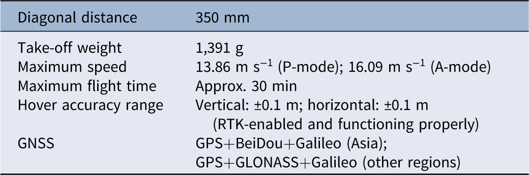
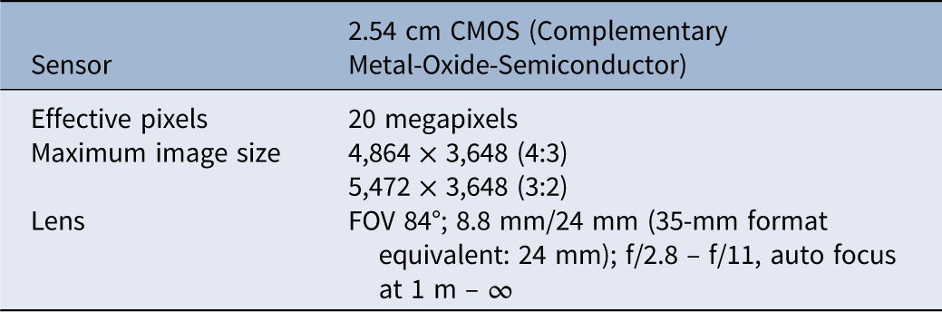
Two commercial wild blueberry fields were selected for this paper in 2025. Site A was located in Union, ME (44.19434°N, 69.31625°W) in the Maine Midcoast growing region. Site B was located in Addison, ME (44.62064°N, 67.70709°W) in the Maine Downeast growing region. Aerial images from each field were taken using a DJI Phantom 4 real-time kinematic (RTK) (DJI, SZ DJI Technology, Shenzhen, China) (Table 1) equipped with an RGB sensor (Table 2), capturing images of red (594 ± 32.5 nm), green (532 ± 58 nm), and blue (468 ± 47 nm) bands. An RGB sensor was used due to its cost-effectiveness (Panduangnat et al. Reference Panduangnat, Posom, Saikaew, Phuphaphud, Wongpichet, Chinapas, Sukpancharoen and Saengprachatanarug2024), similar usefulness with multispectral cameras (Bilodeau et al. Reference Bilodeau, Esau, MacEachern, Farooque, White and Zaman2023; Svensgaard et al. Reference Svensgaard, Jensen, Christensen and Rasmussen2021), and ability to capture the contrast of colors between weeds and non-weeds in early prune year fields. The camera was pointed at nadir (90°) and all flight paths were in a single grid with parallel flight lines, oriented to follow the longest dimension of each study site. The aerial images were taken on May 20, 2025, when emerged weeds were between 8- and 23-cm tall during the early prune year of the crop. The weeds captured were generalized and represented all weeds present at Sites A and B. Flights were taken at an altitude of 41.15 m above ground level (AGL) with an 80% forward and side overlap as modified from the study of Bilodeau et al. (Reference Bilodeau, Esau, MacEachern, Farooque, White and Zaman2023). The resulting ground sample distance (GSD) was 1 cm per pixel for Sites A and B. The terrain following was enabled for each flight. Three ground control points (GCPs) were placed at Site A and two were placed at Site B. These were used to fine-tune the RTK corrections of the DJI Phantom 4 RTK drone. The aerial images were processed using Agisoft Metashape Professional (Agisoft v. 2.1.0, St Petersburg, Russia) to create an orthomosaic of the study areas. Geometric corrections utilized the Maine Department of Transportation Continuously Operating Reference Station (DOT CORS) network: the MEWA station code for Site A and the MEMA station code for Site B. Control was placed using a Leica Zeno GG04 Smart Antenna (Leica Geosystems, Heerbrugg, Switzerland) connected in RTK mode for both sites.
Specifications of the DJI Phantom 4 RTK drone used for imaging.

Table 1. Long description
A table with six rows and two columns. The first column lists specifications and the second column lists corresponding values. Row 1: Diagonal distance, 350 millimeters. Row 2: Take-off weight, 1,391 grams. Row 3: Maximum speed, 13.86 meters per second in P-mode and 16.09 meters per second in A-mode. Row 4: Maximum flight time, approximately 30 minutes. Row 5: Hover accuracy range, vertical plus or minus 0.1 meters and horizontal plus or minus 0.1 meters with RTK-enabled and functioning properly. Row 6: GNSS, GPS plus BeiDou plus Galileo in Asia and GPS plus GLONASS plus Galileo in other regions.
Specifications of the Phantom 4 Pro RGB camera mounted on the DJI Phantom 4 RTK drone.

Table 2. Long description
A table with two rows and four columns detailing the specifications of a camera sensor and lens. The first row lists the sensor type as a 2.54 cm CMOS with 20 megapixels of effective pixels. The maximum image size is 4,864 x 3,648 (4:3) and 5,472 x 3,648 (3:2). The lens has a FOV of 84 degrees with an 8.8 mm focal length, equivalent to 24 mm in 35-mm format, and a range of f/2.8 to f/11 with auto focus from 1 meter to infinity.
Raster Histogram
Raster histograms were generated following a modified version of the methodology of Panduangnat et al. (Reference Panduangnat, Posom, Saikaew, Phuphaphud, Wongpichet, Chinapas, Sukpancharoen and Saengprachatanarug2024). In ArcGIS® Pro (ArcGIS® Pro v. 3.2.0, ESRI, Redlands, CA, USA), 20 representative rectangular polygons were assigned for each class: weed and non-weed. The Histogram tool was then applied to calculate the frequency distribution across all spectral bands for each class. The extracted data were subsequently exported as tables and visualized in RStudio (v. 2025.05.1, PBC, Boston, MA, USA).
Image Classification
Ground Spot Spraying
Image classification was conducted using PIX4Dfields (PIX4D S.A. v. 2.9.5, Prilly, Switzerland). The Boundary tool was first applied to define the sprayer’s operational area, and the Obstacle tool identified field obstacles to avoid during spot spraying. Two mapping workflows were used: the “Magic Tool” and the Index Tool workflow. In the “Magic Tool” workflow, pixels were assigned to the classes “wanted” (weed) and “unwanted” (non-weed). Grid-based classification was generated automatically by selecting a minimum of 50 training samples (representative pixels) per class (Congalton Reference Congalton1991; Figure 2), with grid cell sizes of 0.37 m2 and 0.84 m2 for Sites A and B, respectively. These were the minimum grid cell size allowed by the software for each site. The grid classification was refined using a cell size of 0.09 m2 without buffers, allowing manual addition or removal of pixels in each class during the cleanup process. Finally, the Operations tool converted the refined grid classification into generic tractor/sprayer GeoTIFF files compatible with John Deere and Agrifac tractor terminals.
The “Magic Tool” grid classification to classify weeds (blue highlighted squares) and non-weeds (not highlighted squares). Weed training samples (blue circles) and non-weed training samples (yellow circles).

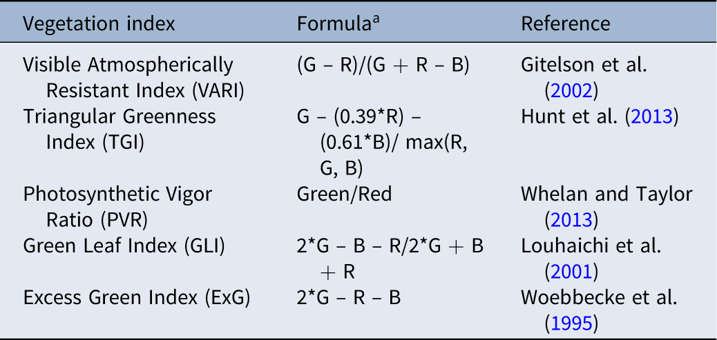
In the Index Tool workflow, five vegetation indices were calculated: Visible Atmospherically Resistant Index (VARI), Triangular Greenness Index (TGI), Photosynthetic Vigor Ratio (PVR), Green Leaf Index (GLI), and Excess Green Index (ExG) (Table 3). These indices were chosen and further studied for their ability to capture the green and white-to-brown color of weeds in the drone imagery. A histogram equalization was utilized due to its contrasting effect (Panduangnat et al. Reference Panduangnat, Posom, Saikaew, Phuphaphud, Wongpichet, Chinapas, Sukpancharoen and Saengprachatanarug2024) and availability in the workflow. Weed patches were highlighted by selecting a specific range of vegetation index values that represented all the weeds in the image. Afterward, the zonation workflow was used in the operations tool to pre-fill the index layer, with different pixel exclusion thresholds applied. Exclusion levels of 10%, 15%, 20%, 25%, and 30% were tested for both Sites A and B as modified from the study of López-Granados et al. (Reference López-Granados, Torres-Sánchez, Serrano-Pérez, De Castro, Mesas-Carrascosa and Peña-Barragán2016). After pixel exclusion, the zone detail was set to “fine,” and the resulting index layers were exported as generic tractor/sprayer GeoTIFF files compatible with John Deere and Agrifac tractor terminals (Figure 3).
List of vegetation indices under study.

Table 3. Long description
A table comparing five vegetation indices. The table has three columns: Vegetation index, Formula, and Reference. The Vegetation index column lists Visible Atmospherically Resistant Index (VARI), Triangular Greenness Index (TGI), Photosynthetic Vigor Ratio (PVR), Green Leaf Index (GLI), and Excess Green Index (ExG). The Formula column provides the mathematical expressions for each index. The Reference column cites the sources for each index. Row 1: Visible Atmospherically Resistant Index (VARI), (G - R)/(G + R - B), Gitelson et al. (2002). Row 2: Triangular Greenness Index (TGI), G - (0.39*R) - (0.61*B)/max(R, G, B), Hunt et al. (2013). Row 3: Photosynthetic Vigor Ratio (PVR), Green/Red, Whelan and Taylor (2013). Row 4: Green Leaf Index (GLI), 2*G - B - R/2*G + B + R, Louhaichi et al. (2001). Row 5: Excess Green Index (ExG), 2*G - R - B, Woebbecke et al. (1995).
a Green (G), red (R), and blue (B) are the values of each band.
Flowchart showing inputs, outputs, and processing steps in PIX4Dfields and ArcGIS Pro Software to make weed maps.

Drone Zone Spraying
Drone zone-spraying maps were generated using two classification methods in PIX4Dfields. A common preprocessing step for both methods involved defining the boundary and field obstacles. The first method utilized the “Magic Tool” to generate a grid classification. Training samples were at least 50 per class (Congalton Reference Congalton1991). The smallest allowable grid cell sizes, 0.37 m2 and 0.84 m2, were used for Sites A and B, respectively. After grid classification, all weed patches were manually digitized in the cleanup process to meet a minimum weed patch size of 405 m2, spaced at least 12 m apart. A 12-m distance between patches was chosen as observed from past drone targeted-spraying missions, and a minimum 405-m2 patch size was a modified version from the studies of Lew-Kowal et al. (Reference Lew-Kowal, Robinson, Gilbert and Rooney2025) and Takekawa et al. (Reference Takekawa, Hagani, Edmunds, Collins, Chappell and Reynolds2023). The second method followed the same procedure in creating the grid classification. However, instead of manually digitizing the weed patches to a minimum of 405 m2, the minimum weed patch size was 9.3 m2 following the methods of Panduangnat et al. (Reference Panduangnat, Posom, Saikaew, Phuphaphud, Wongpichet, Chinapas, Sukpancharoen and Saengprachatanarug2024) and the advice of licensed Maine drone operators at the time of weed map creation (Active Intelligence, personal communication, June 18, 2024). Finally, all resulting classifications were exported as GeoTIFF files compatible with the DJI Agras Mission drone (T-series) (Figure 3).
Accuracy Assessments
All maps generated were evaluated using both image-based and ground-based accuracy assessments in ArcGIS® Pro. One hundred accuracy assessment points were generated using the stratified random sampling technique and served as reference data. The sample size was determined based on sample size determination of Bilodeau et al. (Reference Bilodeau, Esau, MacEachern, Farooque, White and Zaman2023). The generated points were used to compare pixels from the original image and pixels from the classified map. Image-based accuracy assessments were based on reference data from the generated drone orthomosaic, while ground-based accuracy assessments were based on reference data on the actual field. Ground-based reference data were generated by importing the same 100 accuracy assessment points used in image-based accuracy assessments as Keyhole Markup Language (KML) files into the Trimble TDC600 handheld device downloaded with the Avenza Mobile Application (v. 5.3.3, Avenza Systems, Toronto, Canada). The device was connected to the Trimble R2 GNSS receiver (Trimble, Westminster, CO, USA), and both were used to geographically locate the points and generate ground-based reference data in the actual field. To achieve centimeter-level vertical and horizontal accuracy, the Trimble R2 GNSS Receiver was corrected using the Maine DOT CORS network using a hotspot. All maps and feature classes were projected to NAD 1983 (2011) UTM Zone 19 before conducting accuracy assessments (Figure 3).
Confusion Matrix Calculations
A confusion matrix was calculated to compare the classified map with the reference data. The following were calculated for the creation of the confusion matrix:
-
1. Producer’s and user’s accuracies. The user’s accuracy is the probability that a pixel classified on the map actually represents the category on the ground. It measures the reliability of the map and Type I error. Meanwhile, the producer’s accuracy is the probability of a reference pixel being correctly classified. It measures the completeness of the classification and Type II error. Two classes, weed and non-weed, were calculated with the user’s and producer’s accuracies. To calculate the user’s and producer’s accuracies, Equations 1–4 were used, where true positive is the total number of correctly classified weed pixels, true negative is the total number of correctly classified non-weed pixels, false positive is the total number of pixels that are classified as a weed when they should be a non-weed, and false negative is the total number of pixels that are classified as non-weed when they should be a weed.
([1]) ${\rm{User's\;accuracy\;of\;the\;weed\;class}}\;{\rm{\;}} \\\;\;\;= {{{{\rm{True\;Positive\;}}}}\over{{{\rm{True\;Positive}} + {\rm{False\;Positive}}}}} \times 100$
([2])
${\rm{Producer's\;accuracy\;of\;the\;weed\;class\;}} \\\;\;\;= {{{{\rm{True\;Positive}}}}\over{{{\rm{True\;Positive}} + {\rm{False\;Negative}}}}} \times 100$
([3])
${\rm{User's\;accuracy\;of\;the\;non - weed\;class\;\;}} \\\;\;\;= {{{{\rm{True\;Negative\;}}}}\over{{{\rm{True\;Negative}} + {\rm{False\;Negative}}}}} \times 100$
([4])
${\rm{\;Producer's}}\;{\rm{accuracy\;of\;the\;non - weed\;class\;}} \\\;\;\;= {{{{\rm{True\;Negative}}}}\over{{{\rm{True\;Negative}} + {\rm{False\;Positive}}}}} \times 100$
-
2. Overall accuracy. The overall accuracy represents the proportion of predictions that the model made correctly. To calculate the overall accuracy, Equation 5 was used, where true positive and true negative are the total number of correctly classified pixels, while false positive and false negative are the total number of incorrectly classified pixels.
([5])
$\begin{align}{\rm{Overall}}\;{\rm{accuracy}} = &\;{{{\rm{True}}\;{\rm{Positive}};+ {\rm{True}}\;{\rm{Negative}}} \over \matrix{ {\rm{True}}\;{\rm{Positive}}\;+ {\rm{True}}\;{\rm{Negative}} \hfill \cr + {\rm{False}}\;{\rm{Positive}}\;+ {\rm{False}}\;{\rm{Negative}} \hfill \cr} } \\&\times 100\end{align}$
-
3. Kappa coefficient. The kappa coefficient shows the overall assessment of the accuracy of the classification. It quantifies the level of agreement among the classified pixels and the reference data. The kappa coefficient can range from −1 to 1. A value of 0 indicates that the classification is no better than a random classification. McHugh (Reference McHugh2012) guidelines provide a framework for interpreting kappa coefficients based on Cohen’s kappa. These guidelines suggest the following interpretations: 0 to 0.20 means no agreement, 0.21 to 0.39 is minimal agreement, 0.40 to 0.59 is weak agreement, 0.60 to 0.79 is moderate agreement, 0.80 to 0.90 is strong agreement, and >0.90 is almost perfect agreement. For the kappa coefficient, Equation 6 was used, where K is the kappa coefficient, i is the class number, N is the total number of classified values compared with truth values,
${{\rm{m}}_{{\rm{i}},{\rm{i}}}}$
is the number of values belonging to the truth class i that have also been classified as class i (i.e., values found along the diagonal of the confusion matrix),
${{\rm{C}}_{\rm{i}}}$
is the total number of predicted values belonging to class i, and
${{\rm{G}}_{\rm{i}}}$
is the total number of truth values belonging to class i.([6])
$\;\;\;{\rm{K}} = \;{{{N\mathop \sum \nolimits_{i =1}^n {m_{i,i}} - \mathop \sum \nolimits_{i = 1}^n \left( {{G_i}{C_i}} \right)}}\over {{{N^2} - \;\mathop \sum \nolimits_{i = 1}^n \left( {{G_i}{C_i}} \right)}}}$


Weed Survey
The weed survey was conducted using the modified version of the simple random sampling using the random number technique from Nkoa et al. (Reference Nkoa, Owen and Swanton2015). Twenty 1 by 1 m quadrats were placed randomly across Sites A and B. The sample size was determined using the sample size equation from the study of Nkoa et al. (Reference Nkoa, Owen and Swanton2015) with a 10% margin of error. Each field was divided into 12 by 12 m grid cells using the Create Fishnet tool found in ArcGIS® Pro, with each grid cell labeled with a number. Twenty grid cells were randomly selected by generating random numbers from Microsoft Excel (v. 2511, Microsoft, Redmond, WA, USA). Those 20 grid cells served as the area where the quadrat was placed. Within the quadrat, weed species, weed count, and weed cover were recorded. Some weed species were too difficult to identify to the species level and were therefore identified to genus. The weed cover of the identified weeds was ranked using the following scale, 1 = 1% to 20%, 2 = 20% to 40%, 3 = 40% to 60%, 4 = 60% to 80%, and 5 = 80% to 100%. Moreover, analysis of similarity (ANOSIM) was carried out to test dissimilarity among existing weed species at Sites A and B using weed cover as an abundance measure.
The following quantitative analysis parameters in weed surveys were calculated:
-
1. Mean density. This refers to the number of weed species in each quadrat. Equation 7 shows the formula for calculating mean density, where
${D_i}$
is the density of the species i,
${\rm{\Sigma }}{Y_i}$
is the number of individual plants of species i contained in the quadrat, and
${S_a}$
is the surface area of the quadrat.([7])
$D_i = {{{{{\Sigma }{Y_i}}}}\over{{{S_a}}}}$
-
2. Frequency. This is the proportion of quadrats containing the weed species. Equation 8 shows the formula for calculating frequency, where
${{{F}}_{{i}}}$
is the frequency value of the species i,
${\rm{\Sigma }}{{{Z}}_{{i}}}$
is the number of quadrats with species i, and
${{n\;}}$
is the total number of quadrats.([8])
${F_i} = {{{{\rm{\Sigma }{\it Z_i}}}}\over{n}}$
-
3. Mean cover. This is the area of the ground covered by the weed species as viewed from above. Equation 9 shows the formula for calculating mean cover, where
${{{C}}_{{i}}}$
is the mean coverage of the species i,
${\rm{\Sigma }}{{\rm{C}}_{\rm{i}}}$
is the estimated percentage cover of species i per quadrat, and
${{n\;}}$
is the total number of quadrats.([9])
${C_i} = {{{{\rm{\Sigma }{\it C_i}}}}\over{n}}$


Results and Discussion
Raster Histogram of RGB Bands
Weed maps that differentiate between weeds and non-weeds in wild blueberry fields were successfully made using RGB drone aerial imagery taken during late May, the time when weeds just started to emerge. The weed maps were able to distinguish the green and white-to-brown color of weeds versus the reddish brown color of non-weeds. This was because the raster histograms of weeds and non-weeds showed differences in both pixel frequency and band overlap. As shown in Figure 4, weed pixels exhibited higher frequencies with an overlap in the red–green bands, whereas non-weed pixels displayed lower frequencies than the weed pixels with an overlap in the blue–green bands. The results supported the findings of Panduangnat et al. (Reference Panduangnat, Posom, Saikaew, Phuphaphud, Wongpichet, Chinapas, Sukpancharoen and Saengprachatanarug2024), in which divergence or overlap of red, green, and blue bands revealed the difference between weeds and non-weeds on the field. The difference in spectral signatures made it possible to generate weed maps at Sites A and B.
Raster histogram of red, green, and blue bands of weeds and non-weeds at Site A (A and B) and Site B (C and D).

Ground Spot-spraying Maps
Image-based accuracy assessments of ground spot-spraying maps produced high overall accuracies of 98% and 91% for Sites A and B, respectively. Meanwhile, ground-based accuracy assessments resulted in lower overall accuracies of 86% and 83% for Sites A and B, respectively. Kappa coefficients indicated strong to almost perfect agreement for image-based assessments and moderate agreement for ground-based assessments (McHugh Reference McHugh2012). For Site A, the confusion matrix from the image-based accuracy assessment showed similar rates of Type I and Type II errors. Under ground-based accuracy assessment, classification performance was higher for non-weed than weed classes, with user’s and producer’s accuracies of 87% and 84%, respectively. In contrast, the confusion matrix for Site B indicated greater misclassification during ground-based assessment, resulting in reduced user’s and producer’s accuracies for both classes (Table 4).
Accuracy assessment of ground spot-spraying weed maps using the PIX4Dfields Magic Tool workflow at Sites A and B.

Table 4. Long description
A table comparing accuracy assessments of ground spot-spraying weed maps at Sites A and B. The table has six rows and six columns. Column headers are Site, Type of accuracy assessment, Classes, User’s accuracy, Producer’s accuracy, Overall accuracy, and Kappa coefficient. Row labels are Site A Image-based, Site A Ground-based, Site B Image-based, and Site B Ground-based. For Site A, Image-based assessment shows 98 percent User’s accuracy and Producer’s accuracy for Weed and Non-weed classes, with 98 percent Overall accuracy and 0.96 Kappa coefficient. Ground-based assessment shows 84 percent User’s accuracy for Weed, 87 percent for Non-weed, 84 percent Producer’s accuracy for Weed, 87 percent for Non-weed, 86 percent Overall accuracy, and 0.72 Kappa coefficient. For Site B, Image-based assessment shows 89 percent User’s accuracy for Weed, 93 percent for Non-weed, 94 percent Producer’s accuracy for Weed, 88 percent for Non-weed, 91 percent Overall accuracy, and 0.82 Kappa coefficient. Ground-based assessment shows 84 percent User’s accuracy for Weed, 82 percent for Non-weed, 85 percent Producer’s accuracy for Weed, 80 percent for Non-weed, 83 percent Overall accuracy, and 0.66 Kappa coefficient.
Ground spot-spraying weed maps generated using the PIX4Dfields “Magic Tool” workflow demonstrated that the HITL-ML algorithm was able to distinguish weeds from non-weeds in Maine wild blueberry fields. The interactive machine learning component of HITL-ML, where humans are actively involved in correctly supplying information to the model, produced comparable overall weed map accuracies based on image-based accuracy assessment (≤98%) to those reported by Bilodeau et al. (Reference Bilodeau, Esau, MacEachern, Farooque, White and Zaman2023) (≤97%), who used supervised image classification workflows in the ArcGIS® Pro software and the same image-based accuracy assessment approach. In addition, overall accuracies from image-based assessments for Site A were consistent with Betitame et al. (Reference Betitame, Igathinathane, Howatt, Mettler, Koparan and Sun2025), López-Granados et al. (Reference López-Granados, Torres-Sánchez, Serrano-Pérez, De Castro, Mesas-Carrascosa and Peña-Barragán2016), and Seiche et al. (Reference Seiche, Wittstruck and Jarmer2024), who reported nearly 100% overall accuracies when discriminating weeds from crops using multispectral sensors. These findings suggest that the RGB sensors used in this study can generate weed maps comparable to those derived from multispectral imagery, supporting the conclusion of Bilodeau et al. (Reference Bilodeau, Esau, MacEachern, Farooque, White and Zaman2023) that RGB imagery is sufficient for weed–crop classification in wild blueberry fields.
Higher accuracies were achieved when the map was assessed using image-based reference data rather than ground-based reference data. This increase is likely due to observer bias during image-based ground truthing. When reference data were generated from the same aerial perspective as the model’s input, subtle features and obscured weeds might have been frequently overlooked. Thus, even though image-based reference data produced high overall accuracies and were mostly used for weed map assessments in previous studies, relying on ground-based reference data was more accurate, as they were collected in the actual field (Lu and Weng Reference Lu and Weng2007).
The decrease in overall accuracies and kappa coefficients of weed maps when using more accurate ground truth reference data revealed misclassification between weeds and non-weeds. This discrepancy was primarily attributable to the spatial resolution during image classification. When weed sizes are smaller than the cells used for grid classification (0.37 m2 and 0.84 m2), the spectral signature of the weed is averaged with the non-weed class (bare soil or crop). This results in “mixed pixels” that the model cannot reliably resolve (Ubben et al. Reference Ubben, Pukrop and Jarmer2024). Furthermore, site-specific noise, specifically the white-gray ash residues from burn pruning, introduced spectral confusion. The high reflectance of the ash mimics the brightness values of certain weed species, leading to false positives in the classification output (Lu and Weng Reference Lu and Weng2007) and lower map accuracy results. However, despite these lower values, the overall accuracies from ground-based reference data (83% to 86%) remained consistent with established research by Peña et al. (Reference Peña, Torres-Sánchez, de Castro, Kelly and López-Granados2013) and Sapkota et al. (Reference Sapkota, Singh, Cope, Valasek and Bagavathiannan2020), who reported similar accuracy thresholds when subjected to the same ground-based validation protocols. Thus, our findings suggest that even though ground-based accuracy assessments result in lower reported map accuracies, they are inherently more accurate in identifying the true presence of weeds.
Vegetation indices (VIs) tested using the Index Tool workflow to create weed maps for ground spot spraying resulted in lower overall accuracies and kappa coefficients than the “Magic Tool” workflow, except for TGI, which had similar overall accuracies (Figure 5). TGI was the most accurate index in all ground-based assessments, reaching accuracies up to 84% for Site A and 85% for Site B. For image-based accuracy assessments, the highest accuracies were achieved by TGI and GLI at Site A and ExG and GLI at Site B. TGI and GLI achieved 93% and 90% overall accuracies, respectively, for Site A, while ExG and GLI reached 88% and 89% overall accuracies, respectively, for Site B. Image-based accuracy assessments also resulted in higher overall accuracies than ground-based assessments, supporting previous results. At the same time, the peak accuracies of the vegetation indices tested were reached at different pixel exclusion levels. For most of the better-performing indices, overall accuracy tended to improve as the exclusion level increased from 10%, typically peaking or plateauing between 20% and 25% (Figure 5).
Overall accuracies by pixel exclusion level of weed maps using the index layer workflow at Sites A and B. ExG, Excess Green Index; GLI, Green Leaf Index; PVR, Photosynthetic Vigor Ratio; TGI, Triangular Greenness Index; VARI, Visible Atmospherically Resistant Index.

Focusing on ground-based accuracy assessments, the TGI had the highest overall accuracy (≤85%), because TGI focuses on chlorophyll and the physiological status of the vegetation (Hunt et al. Reference Hunt, Doraiswamy, McMurtrey, Daughtry, Perry and Akhmedov2013) and not on color alone (Starý et al. Reference Starý, Jelínek, Kumhálová, Chyba and Balážová2020). ExG emphasizes on “greenness” and differentiates green vegetation from soil (Woebbecke et al. Reference Woebbecke, Meyer, Von Bargen and Mortensen1995), while GLI is similar to ExG but has a normalization step to account for varying light conditions (Louhaichi et al. Reference Louhaichi, Borman and Johnson2001). PVR and VARI did not perform well compared with the other indices, perhaps because both focused their calculations on the green and red bands alone, with VARI using the blue band only for normalization. The blue band was essential to consider in the index calculation, as it was observed that a blue–green band overlap was present on non-weed pixels (Figure 4B and D). Overall, TGI was the most promising VI for overall weed detection in wild blueberry fields during late May.
The ground-based overall accuracies of the VIs tested were similar to the findings of Percival et al. (Reference Percival, Anku and Langdon2023), in which visible light indices reached 83% classification accuracy when mapping diseased wild blueberry plants using ground truth reference data. Meanwhile, higher overall accuracies achieved at 20% to 25% pixel exclusion suggested that removing a moderate percentage of pixels for all VIs tested enhances classification accuracy during zonation. This result supported López-Granados et al. (Reference López-Granados, Torres-Sánchez, Serrano-Pérez, De Castro, Mesas-Carrascosa and Peña-Barragán2016), who observed that increasing weed thresholds (higher pixel exclusion level) increased classification accuracy. However, classification accuracy decreased or plateaued after optimal thresholds were reached, indicating that removing too many weed pixels may lower map accuracy results.
Drone Zone-spraying Maps
As expected, drone zone-spraying maps having a 405-m2 weed patch size had lower overall accuracies and kappa coefficients when compared with high-performing maps made for ground spot spraying (Table 5). The resulting overall accuracies were 78% (image-based) and 77% (ground-based) for both Sites A and B. In contrast, reducing the minimum weed patch size to 9.3 m2 significantly improved performance at Site A, yielding overall accuracies of 88% (image-based) and 86% (ground-based), while Site B had overall accuracies of 75% (image-based) and 74% (ground-based) (Table 6). While the overall accuracies for Site A with a 9.3-m2 threshold were considered acceptable for wild blueberry research (Percival et al. Reference Percival, Anku and Langdon2023), they were slightly lower than those from the grid-based mapping by Panduangnat et al. (Reference Panduangnat, Posom, Saikaew, Phuphaphud, Wongpichet, Chinapas, Sukpancharoen and Saengprachatanarug2024), which also used an approximately 9.3-m2 weed patch size threshold. This discrepancy may be potentially due to Panduangnat et al.’s (Reference Panduangnat, Posom, Saikaew, Phuphaphud, Wongpichet, Chinapas, Sukpancharoen and Saengprachatanarug2024) hexagonal grid cells or a different number of assessment points used as reference data.
Accuracy assessment of drone zone-spraying weed maps developed in PIX4Dfields with a minimum 405-m2 weed patch size at Sites A and B.

Table 5. Long description
A table comparing accuracy assessments of drone zone-spraying weed maps at two sites. The table has six rows and six columns. Column headers are Site, Type of accuracy assessment, Classes, User’s accuracy, Producer’s accuracy, Overall accuracy, and Kappa coefficient. Row labels are Site A Image-based Weed, Site A Image-based Non-weed, Site A Ground-based Weed, Site A Ground-based Non-weed, Site B Image-based Weed, Site B Image-based Non-weed, Site B Ground-based Weed, and Site B Ground-based Non-weed. Row 1: Site A, Image-based, Weed, 69 percent, 91 percent, 78 percent, 0.57. Row 2: Site A, Image-based, Non-weed, 90 percent, 67 percent, 78 percent, 0.57. Row 3: Site A, Ground-based, Weed, 68 percent, 91 percent, 77 percent, 0.55. Row 4: Site A, Ground-based, Non-weed, 90 percent, 65 percent, 77 percent, 0.55. Row 5: Site B, Image-based, Weed, 74 percent, 88 percent, 78 percent, 0.56. Row 6: Site B, Image-based, Non-weed, 84 percent, 67 percent, 78 percent, 0.56. Row 7: Site B, Ground-based, Weed, 73 percent, 88 percent, 77 percent, 0.54. Row 8: Site B, Ground-based, Non-weed, 84 percent, 65 percent, 77 percent, 0.54.
Accuracy assessment of drone zone-spraying weed maps developed in PIX4Dfields with a minimum 9.3-m2 weed patch size at Sites A and B.

Table 6. Long description
A table comparing accuracy assessments of drone zone-spraying weed maps at two sites. The table has six rows and six columns. Column headers are Site, Type of accuracy assessment, Classes, User’s accuracy, Producer’s accuracy, Overall accuracy, and Kappa coefficient. Row labels are Site A Image-based Weed, Site A Image-based Non-weed, Site A Ground-based Weed, Site A Ground-based Non-weed, Site B Image-based Weed, Site B Image-based Non-weed, Site B Ground-based Weed, and Site B Ground-based Non-weed. Row 1: Site A, Image-based, Weed, 84 percent, 91 percent, 88 percent, 0.76. Row 2: Site A, Image-based, Non-weed, 92 percent, 85 percent, 88 percent, 0.76. Row 3: Site A, Ground-based, Weed, 82 percent, 89 percent, 86 percent, 0.72. Row 4: Site A, Ground-based, Non-weed, 90 percent, 84 percent, 86 percent, 0.72. Row 5: Site B, Image-based, Weed, 72 percent, 85 percent, 75 percent, 0.50. Row 6: Site B, Image-based, Non-weed, 79 percent, 65 percent, 75 percent, 0.50. Row 7: Site B, Ground-based, Weed, 70 percent, 84 percent, 74 percent, 0.48. Row 8: Site B, Ground-based, Non-weed, 79 percent, 63 percent, 74 percent, 0.48.
The generalization observed in drone zone-spraying maps was necessitated by the spray drone’s minimum weed patch size requirements. Unlike ground-based tractor sprayers, which can spray targets greater than the 0.25-m2 threshold (Bilodeau et al. Reference Bilodeau, Esau, MacEachern, Farooque, White and Zaman2023), agricultural spray drones, particularly DJI Agras drones, generally require larger patch sizes (ranging from 9.3 m2 to 405 m2) due to the spray drone’s wider spray width pattern (Byers et al. Reference Byers, Virk, Rains and Li2024; DJI 2025). Meanwhile, even though the 9.3-m2 threshold achieved similar ground-based accuracy assessments with ground spot-spraying maps, its success was highly dependent on site characteristics. Hunter et al. (Reference Hunter, Gannon, Richardson, Yelverton and Leon2020) found that drone weed detection increased with weed patch aggregation. The results support this, as the aggregated weeds present at Site A allowed for clear patch delineation, resulting in high map accuracies. Conversely, the uniform weed distribution found at Site B made generalization subjective, reducing accuracy of the 9.3-m2 threshold compared with the 405-m2 threshold (Tables 5 and 6).
Ultimately, the generalization inherent in zone spraying, which excludes weeds below a certain size, led to more generalized weed polygons than ground spot-spraying maps (Figures 6 and 7), and therefore achieved lower map accuracies. However, this generalization was needed to cover the spray drone’s optimal spray widths while allowing for spot-spraying applications to occur (Hunter et al. Reference Hunter, Gannon, Richardson, Yelverton and Leon2020; Panduangnat et al. Reference Panduangnat, Posom, Saikaew, Phuphaphud, Wongpichet, Chinapas, Sukpancharoen and Saengprachatanarug2024). The smaller weed patch size threshold of 9.3 m2 produced weed maps with comparable performance from ground spot-spraying maps, especially in fields with clustered weed populations. However, the results were site dependent, as Site B resulted in lower overall map accuracies than Site A. Thus, further research on weed patch size thresholds on different weed distributions is warranted.
Weed maps of Site A: (A) RGB color image, (B) ground spot-spraying map using the Magic Tool workflow, (C) drone zone-spraying map with a minimum 9.3-m2 weed patch size, and (D) drone zone-spraying map with a minimum of 405-m2 weed patch size.

Weed maps of Site B: (A) RGB color image, (B) ground spot-spraying map using the Magic Tool workflow, (C) drone zone-spraying map with a minimum 9.3-m2 weed patch size, and (D) drone zone-spraying map with a minimum of 405-m2 weed patch size.

Weed Survey
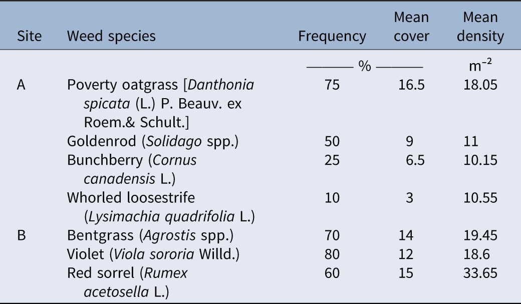
Higher overall accuracies and kappa coefficients were observed at Site A than at Site B in all weed maps tested in this paper. This showed that there was more misclassification of grid pixels at Site B than at Site A. One factor that may have contributed to misclassification was the weed species composition and abundance. At Site A, the total weed coverage was 1.08 and 1.46 ha, while Site B had a weed coverage of 1.88 and 2.00 ha from representative ground and drone zone-spraying maps, respectively. These resulted in ground and drone zone-spraying map weed percentages of 39.00% and 58.00% for Site A and 52.17% and 61.29% for Site B, respectively (Supplementary Material 1). The weed survey revealed that poverty oatgrass [Danthonia spicata (L.) Beauv. ex Roem. & Schult.] was the most dominant species at Site A, with the highest frequency (75%), mean density (18 plants m−2), and mean cover (16.5%). Goldenrod (Solidago spp.) followed with a frequency of 50%, mean density of 11 plants m⁻2, and mean cover of 9%. Following Solidago spp., whorled loosestrife (Lysimachia quadrifolia L.) had the next highest mean density of 10.55 plants m−2, while bunchberry (Cornus canadensis L.) ranked next in terms of frequency (25%) and mean cover (6.5%). At Site B, red sorrel (R. acetosella L.), bentgrass (Agrostis spp.), and violet (Viola sororia Willd.) had the highest mean densities (33.65, 19.45, and 18.60 plants m⁻², respectively). In terms of frequency, V. sororia (80%), Agrostis spp. (70%), and R. acetosella (60%) were the most widespread. R. acetosella also had the highest mean cover, followed by Agrostis spp. and V. sororia (Table 7). In total, 12 weed species were recorded at Site A. Site B, having 26 observed weed species, exhibited greater weed species diversity than Site A. ANOSIM revealed a significant difference in species composition between Sites A and B (R = 0.555, P = 0.001). The separation between groups was moderate to strong, with between-group dissimilarities consistently exceeding within-group variation.
List of weed species representing the three highest values of frequency, mean density, and mean cover at each study site.

Table 7. Long description
A table comparing weed species frequency, mean cover, and mean density at two study sites. The table has two rows labeled A and B, representing the two sites. Each row contains data for three weed species with the highest values of frequency, mean cover, and mean density. Column headers are Site, Weed species, Frequency (percent), Mean cover (percent), and Mean density (plants per square meter). Row A: Poverty oatgrass [Danthonia spicata (L.) P. Beauv. ex Roem. & Schult.], Frequency 75, Mean cover 16.5, Mean density 18.05. Goldenrod (Solidago spp.), Frequency 50, Mean cover 9, Mean density 11. Bunchberry (Cornus canadensis L.), Frequency 25, Mean cover 6.5, Mean density 10.15. Whorled loosestrife (Lysimachia quadrifolia L.), Frequency 10, Mean cover 3, Mean density 10.55. Row B: Bentgrass (Agrostis spp.), Frequency 70, Mean cover 14, Mean density 19.45. Violet (Viola sororia Willd.), Frequency 80, Mean cover 12, Mean density 18.6. Red sorrel (Rumex acetosella L.), Frequency 60, Mean cover 15, Mean density 33.65.
Because Site A had significantly fewer weed species observed than Site B, this created an environment where weed training samples were more visually uniform, which made it easier for the software to learn and classify. Meanwhile, Site B had more weed species composition, which resulted in more weed pixels having different colors and textures. The results supported the studies of Lu and He (Reference Lu and He2017) and Ronay et al. (Reference Ronay, Lati and Kizel2024), which discussed how color variation and growth progress of the weed species can complicate classification. Heterogeneity of weed pixels made the software more prone to misclassification, while homogeneity of weed pixels increased accuracy. In addition, the weed species present also explained why Site A had more weed aggregation than Site B. D. spicata occurs in clumps through tillering (Navarrete-Tindall and Van Sambeek Reference Navarrete-Tindall and Van Sambeek2010), while Solidago spp. dominantly reproduce through seeds and creeping rhizomes that form large patches and colonies (Neal et al. Reference Neal, Uva, DiTomaso and DiTommaso2023). L. quadrifolia also reproduces via seeds and rhizomes, but the seeds lack a dispersal mechanism and typically fall to the ground near the parent plant (Minnesota Department of Natural Resources 2024). This localized dispersal of propagules may have contributed to the aggregated pattern of Site A. Meanwhile, V. sororia utilizes a ballistic dispersal, forcefully ejecting seeds away from the mother plant (Ohkawara and Higashi Reference Ohkawara and Higashi1994), while R. acetosella produces rhizomes and seeds that can be dispersed by wind, water, and animals, increasing chances for weed seed distribution across greater distances (Löve Reference Löve1983). Unlike D. spicata, which initially occurs in clumps, Agrostis spp. primarily spread by seed (Boyd et al. Reference Boyd, White and Rao2014), leading to the germination of individual seedlings in the field. This may have contributed to less aggregation of weed patches at Site B and thus a more uniform weed spatial distribution leading to less accurate weed maps.
It is also important to recognize that the weed maps generated in this paper distinguished only between weeds and non-weeds, with “weed” broadly defined as any unwanted plant within the crop system. However, in wild blueberry fields, not all non-crop plants are necessarily detrimental. Certain weed species may provide ecological benefits, such as attracting beneficial organisms, supporting biodiversity, and reducing soil erosion (Bagavathiannan and von Redwitz Reference Bagavathiannan and von Redwitz2025). Therefore, the binary classification used in this study generalized all non-crop vegetation as weeds and did not account for differences among individual plant species or their potential ecological functions. Future research should investigate methods for distinguishing potentially beneficial or “neutral” weeds (Esposito et al. Reference Esposito, Westbrook, Maggio, Cirillo and DiTommaso2023) from problematic weeds in wild blueberry fields and evaluate how their presence influences crop production and overall agroecosystem health.
Implications for Growers and Drone Operators
For drone operators planning to use weed maps, RGB drone images processed in PIX4Dfields can successfully map weeds in Maine wild blueberry fields with an overall accuracy of ≤86% based on ground-based reference data and ≤98% based on image-based reference data. The grid classification of the software has insufficient resolution to classify weeds smaller than the smallest allowable grid cell but has compatibility benefits for commercially available sprayers for target weed control. The “Magic Tool” workflow is recommended for creating ground spot-spraying weed maps in PIX4Dfields, due to increased overall accuracies through human intervention in the machine learning process. The TGI Index Tool workflow with the pixel exclusion level of 20% to 25% can be an alternative if time is limited. The site is an important factor to consider, as high weed compositions and uniform weed distribution can lower map accuracies. There is no established minimum weed patch yet for drone zone spraying, but it is recommended to make weed maps with a minimum weed patch size of 9.3 m2 or as wide as the selected drone’s minimum spray width.
Weed coverage for both ground and drone zone-spraying maps reveals that the weeds are ≤61% of the total field area, which suggests herbicide savings up to approximately 40% for all these sites. Growers can purchase their own mapping and spray drones, or they can hire drone services. Drone operators in Maine charged US$350 for each field image flight using either an RGB or multispectral sensor. To apply pesticide, fertilizer or seed, they charged an additional US$61.78 ha−1 (Active Intelligence, personal communication, 2024). Therefore, potential savings from targeted spraying must be weighed against costs from drone mapping and spraying to be considered a valuable weed management tool.
Supplementary material
To view supplementary material for this article, please visit https://doi.org/10.1017/wsc.2026.10154.
Acknowledgments
We thank Paul Sweetland and Courtney Hammond for their support and access to their wild blueberry farms. We also thank David Sandilands from the School of Forest and Natural Resources, University of Maine, for providing the drone aerial imagery for this research. We would also like to thank Active Intelligence, David Handley, and Travis Esau with his graduate student, Chloe Toombs, for providing guidance in this research. Language and graph editing of this manuscript was assisted by ChatGPT 5.2 (OpenAI). The authors reviewed the manuscript and take full responsibility for all content and interpretations.
Funding statement
This research is funded and supported by the University of Maine Cooperative Extension and the Northeast IPM Center (grant no. 2022-70006-38004).
Competing interests
No conflicts of interest have been declared.












 Open access

