2.1 Flow cell and magnetic field

We create a highly turbulent flow in a cylindrical container driven by two counter-rotating discs. The container has an inner radius of $R=5~\text{cm}$ and is mounted vertically. The discs are spaced 10 cm apart and are fitted with 8 straight blades (figure 1). This flow topology, known as von Kármán flow, is widely used in experiments on turbulent flows (Douady, Couder & Brachet Reference Douady, Couder and Brachet1991; Maurer, Tabeling & Zocchi Reference Maurer, Tabeling and Zocchi1994; Voth et al. Reference Voth, La Porta, Crawford, Alexander and Bodenschatz2002; Ravelet et al. Reference Ravelet, Marié, Chiffaudel and Daviaud2004). The flow is globally non-isotropic, and homogeneity applies only in the centre of the flow cell. Due to topological symmetry there is isotropy in the transverse directions, the plane in which we apply the uniform magnetic field. The coordinate system in the flow cell is defined such that the $x_{1}$ – $x_{2}$ plane is in the transverse direction and $x_{3}$ defines the axial direction.

The magnetic field is applied in the direction of $x_{1}$ . It is very homogeneous over the volume of the flow cell (figure 2). We modelled the field using the formulas of Conway (Reference Conway2006) and compared it with the measured values. As the results compare well with the measured magnetic field, the model can be used to estimate the field homogeneity over the whole flow cell, and the field is found to be uniform to within ${\rm\Delta}B/B_{centre}=1500~\text{ppm}$ .

Figure 2.

Axial magnetic field component generated by three coils, (a) along the axis, (b) transverse at mid-height. The solid line shows the modelled magnetic field. Vertical dashed lines indicate the boundaries of the test cell.

Table 1.

Properties of ferrofluid composed of spherical magnetic silica particles.

2.2 Magnetic fluid

The experiments were conducted with an aqueous ferrofluid whose properties are summarised in table 1.

Under zero magnetic field, the fluid behaves as purely Newtonian with density ${\it\rho}_{f}=1.0144~\text{g}~\text{cm}^{-3}$ and viscosity ${\it\eta}_{0}=3~\text{mPa}~\text{s}$ , values that are similar to those of water. Under the influence of an external magnetic field, the particles in the fluid form short linear chains which are preferentially aligned in the field direction. The resulting anisotropic response to shearing motions and its impact on the flow can be conceptualised by a direction dependent viscosity (Ericksen Reference Ericksen1960; Leslie Reference Leslie1966; Ilg & Kröger Reference Ilg and Kröger2002).

We measured the viscosity using a parallel-plate rheometer with the magnetic field perpendicular to the shearing motion. The fluid viscosity is a function of shear rate (figure 3 a) and magnetic field (figure 3 b). The increase in viscosity with magnetic field has been investigated thoroughly (Odenbach Reference Odenbach2004). In figure 3(b) we show this increase for a shear rate of $100~\text{s}^{-1}$ , which is considerably lower than in the actual experiments. According to simulations (Sreekumari & Ilg Reference Sreekumari and Ilg2015) and experiments (Linke & Odenbach Reference Linke and Odenbach2015) of similar chain-forming fluids this viscosity effect is truly anisotropic. The viscosity decrease with increasing shear rate, known as shear thinning, is caused by shear forces that limit the chain length.

Figure 3.

(a) Dynamic viscosity of the ferrofluid as a function of shear rate at different external magnetic field magnitudes and (b) as a function of external magnetic field magnitude for a shear rate $\dot{{\it\gamma}}=100~\text{s}^{-1}$ .

The observed shear thinning has an influence on the achievable viscosity anisotropy. Since the time scales of the turbulent flow are much shorter than the relaxation time scale of chain formation (Borin et al. Reference Borin, Zubarev, Chirikov, Müller and Odenbach2011), the chain length is ultimately determined by the maximum shear rate in the flow cell which is reached near the rotating discs rather than the local shear rate values.

As the fluid is non-conducting there is no magnetic induction and hence no additional bulk force acting on the fluid. A similar rheological anisotropy can be created in some types of liquid crystals, whose flow behaviour is well understood. However, for viscosity-induced effects in liquid crystals, much higher magnetic fields are required as compared to ferrofluids and the higher viscosity makes the creation of a turbulent flow more difficult.

2.3 Flow velocimetry

Since ferrofluids are opaque at optical wavelengths, the flow velocities were measured using ultrasound velocimetry techniques.

As we are primarily interested in the influence of anisotropic small scales on the turbulence cascade, we have to use a measurement technique capable of fully resolving all scales of turbulent motion. Standard ultrasound Doppler velocity profiling (UVP) based on a pulse-echo technique is not suitable because of the highly transient nature of the turbulent flow that has to be sampled with sufficient temporal resolution. The flow fluctuates on time scales down to the Kolmogorov time ${\it\tau}_{{\it\eta}}=4.2~\text{ms}$ .

In addition to UVP we thus use a technique based on continuous ultrasound recording, similar to the one developed by Mordant et al. (Reference Mordant, Metz, Pinton and Michel2005). This is a time resolved measurement technique that tracks the continuous Doppler-shifted scattering signals of tracers moving in the observation volume. Since single tracer particles are being followed in the flow, the technique belongs to the class of Lagrangian particle tracking methods.

The fluid is seeded with a small number of spherical polystyrene particles with a diameter of $d=250~{\rm\mu}\text{m}$ and a density of ${\it\rho}_{p}=1.04~\text{g}~\text{cm}^{-3}$ . As the particle size is not much larger than the Kolmogorov microscale ( $d/{\it\eta}=2.2$ ), tracer-like behaviour can be expected (Brown, Warhaft & Voth Reference Brown, Warhaft and Voth2009). Magnetophoretic forces on the tracer particles are negligible due to the very small magnetic field gradients in the flow cell.

Even though not universally applicable for resolved turbulence measurements, UVP can still provide valuable information about the flow in the test cell. Profiles of the velocity component along different observation directions were recorded with such a system, providing data on the ‘slow’ spatial modes developing in the flow cell and changing under the action of the magnetic field.

3.1 Velocity probability distribution

Figure 4 shows the probability density function of the 3 Lagrangian velocity components in the field-free case. The transverse components exhibit similar statistics as expected from symmetry. The transverse components show a larger standard deviation than the axial component. The probability density functions are close to Gaussian with a kurtosis of 2.7 for the transverse components and 3.7 for the axial component. The kurtosis of the transverse components is in agreement with Voth et al. (Reference Voth, La Porta, Crawford, Alexander and Bodenschatz2002), while for the axial component the kurtosis is slightly larger.

Figure 4.

The velocity PDF at zero field. $u_{1}$ and $u_{2}$ are two orthogonal transverse velocity components and $u_{3}$ is the axial velocity component.

3.2 Second-order structure function

The Lagrangian second-order structure function is defined as the variance of the Lagrangian velocity increments:

(3.1) $$\begin{eqnarray}D_{2}({\it\tau})\equiv \langle [u_{i}(t+{\it\tau})-u_{i}(t)]^{2}\rangle ,\end{eqnarray}$$

where $u_{i}(t)$ is one Lagrangian velocity component. The structure function of a transverse velocity component for the field-free case is shown in figure 5(a). It varies with ${\it\tau}^{2}$ in the dissipation range and approaches a constant value for long time lags. When scaled by ${\it\varepsilon}{\it\tau}$ , this should show a plateau in the inertial subrange. Very high Reynolds numbers are required to see this plateau so we can only see a peak. Nevertheless we can take the maximum value $C_{0}^{\ast }=\max \{D_{2}({\it\tau})/{\it\tau}{\it\varepsilon}\}$ and compare it with published values for comparable Reynolds numbers. Our value is $C_{0}^{\ast }=3.5\pm 0.3$ , which is somewhat smaller than reported values from numerical simulations with $C_{0}^{\ast }=4.4$ at $R_{{\it\lambda}}=140$ (Yeung, Pope & Sawford Reference Yeung, Pope and Sawford2006).

Figure 5.

(a) Compensated Lagrangian second-order structure function as a function of normalised time and (b) Scaling of relative scaling exponents ${\it\zeta}_{p}^{L}/{\it\zeta}_{2}^{L}$ of the structure functions with structure function order $p$ . For comparison we show the data of Mordant, Lévêque & Pinton (Reference Mordant, Lévêque and Pinton2004b ) at $R_{{\it\lambda}}=810$ . The solid line shows the Kolmogorov (Reference Kolmogorov1941) prediction.

Higher-order moments of Lagrangian velocity increments are studied within the scope of Lagrangian intermittency. As the scaling range in Lagrangian structure functions is not established, the scaling of these structure functions is usually investigated by plotting them against the second-order structure function (extended self-similarity (Benzi et al. Reference Benzi, Ciliberto, Tripiccione, Baudet, Massaioli and Succi1993)). To measure relative scaling exponents we fit power laws to the structure functions in the range where the second-order structure function shows a developing inertial range, in our case between $3{\it\tau}_{{\it\eta}}$ and $6{\it\tau}_{{\it\eta}}$ . Our structure functions show scaling similar to the findings of Mordant et al. (Reference Mordant, Lévêque and Pinton2004b ) (figure 5 b).

For a statistically stationary process the velocity autocorrelation function $R({\it\tau})$ is given through the second-order structure function $D_{2}({\it\tau})$ by

(3.2) $$\begin{eqnarray}\displaystyle R({\it\tau}) & \equiv & \displaystyle \langle u(t+{\it\tau})u(t)\rangle /\langle u^{2}\rangle\end{eqnarray}$$

(3.3) $$\begin{eqnarray}\displaystyle & = & \displaystyle 1-\frac{D_{2}({\it\tau})}{2\langle u^{2}\rangle }.\end{eqnarray}$$

The Lagrangian velocity autocorrelation function exhibits an exponential decay with a finite curvature at the origin. This function can be modelled with a second-order model (Sawford Reference Sawford1991) where $T_{L}$ is the Lagrangian integral time scale and $T_{2}$ is a time scale related to dissipation:

(3.4) $$\begin{eqnarray}R({\it\tau})=\frac{T_{L}\exp (-{\it\tau}/T_{L})-T_{2}\exp (-{\it\tau}/T_{2})}{T_{L}-T_{2}}.\end{eqnarray}$$

We fit this model between 0 and ${\it\tau}=10{\it\tau}_{{\it\eta}}$ and obtain the estimates for $T_{L}$ and $T_{2}$ given in table 2. The velocity autocorrelation function is biased for large times as a consequence of the finite measurement volume.

3.3 Accelerations

Accelerations are computed by convolving the velocity trajectories with a differentiated and truncated Gaussian kernel (Mordant, Crawford & Bodenschatz Reference Mordant, Crawford and Bodenschatz2004a ). The kernel width, which corresponds to the standard deviation of the Gaussian, is chosen as ${\it\tau}_{w}=0.25{\it\tau}_{{\it\eta}}$ . This is a compromise between achievable noise reduction and preserved signal bandwidth.

Figure 6.

Lagrangian velocity autocorrelation function against normalised time. The marks show every 10th data point and the solid line is a fit of Sawford’s second-order model.

Figure 7.

(a) The PDF of one transverse acceleration component normalised by its standard deviation. Accelerations are computed by convolving the velocity with a differentiated Gaussian with standard deviation $0.25{\it\tau}_{{\it\eta}}$ . For comparison the PDF of pressure gradients measured in a DNS at $R_{{\it\lambda}}=140$ (Vedula & Yeung Reference Vedula and Yeung1999) is shown. (b) The autocorrelation function of one acceleration component at zero field. The time lag is normalised by the Kolmogorov time ${\it\tau}_{{\it\eta}}$ and the correlation drops below zero around $2.2{\it\tau}_{{\it\eta}}$ .

Figure 7(a) shows the probability density function of one transverse acceleration component. It displays the well-known long tails. For comparison we show the pressure gradient PDF measured in a DNS of Vedula & Yeung (Reference Vedula and Yeung1999) for a similar Reynolds number. Our data follows their results very well.

The Heisenberg–Yaglom relation states

(3.5) $$\begin{eqnarray}\langle a^{2}\rangle =a_{0}{\it\varepsilon}^{3/2}{\it\nu}^{-1/2},\end{eqnarray}$$

with scaling constant $a_{0}$ . Using DNS and experimental data Sawford et al. (Reference Sawford, Yeung, Borgas, Vedula, La Porta, Crawford and Bodenschatz2003) parametrised the constant $a_{0}$ as $a_{0}=1.9R_{{\it\lambda}}^{0.135}/(1+85/R_{{\it\lambda}}^{1.135})$ . From our data we obtain $a_{0}=2.7\pm 0.2$ for one transverse acceleration component while the parametrisation gives a value of 2.64 for the given value of $R_{{\it\lambda}}$ .

Figure 7(b) shows the autocorrelation function of one transverse acceleration component. It has the typical shape with rapid decrease and negative values for long time lags. The zero-crossing time ${\it\tau}_{a}$ is $2.2{\it\tau}_{{\it\eta}}$ , consistent with Yeung & Pope (Reference Yeung and Pope1989).

Estimating energy dissipation is difficult using only single-particle statistics. Commonly one measures spatial second- or third-order velocity structure functions. These show a clear scaling in the inertial range from which ${\it\varepsilon}$ can be estimated. Relying on the acceleration of the trajectories we can instead use the trace of the acceleration–velocity covariance tensor of the fluid particle trajectories:

(3.6) $$\begin{eqnarray}{\it\varepsilon}=-\langle u_{i}a_{i}\rangle ,\end{eqnarray}$$

which is valid for decaying, homogeneous turbulence (Ott & Mann Reference Ott and Mann2005).

3.4 Spectra

The Lagrangian velocity spectrum $E^{L}({\it\omega})$ and acceleration spectrum $A^{L}({\it\omega})$ are given by the cosine transform of the respective autocovariance function (Sawford & Yeung Reference Sawford and Yeung2011).

(3.7) $$\begin{eqnarray}\displaystyle & \displaystyle E^{L}({\it\omega})=\frac{2}{{\rm\pi}}\int _{0}^{\infty }\langle u(t+{\it\tau})u(t)\rangle \cos ({\it\omega}{\it\tau})\,\text{d}{\it\tau} & \displaystyle\end{eqnarray}$$

(3.8) $$\begin{eqnarray}\displaystyle & \displaystyle A^{L}({\it\omega})=\frac{2}{{\rm\pi}}\int _{0}^{\infty }\langle a(t+{\it\tau})a(t)\rangle \cos ({\it\omega}{\it\tau})\,\text{d}{\it\tau}. & \displaystyle\end{eqnarray}$$

One may look at the frequency spectra to see if the scales are sufficiently separated (figure 8). As it is a log–linear plot, we multiply the spectra by ${\it\omega}$ to depict the energy at each scale. The acceleration spectrum peaks around the Lagrangian time microscale ${\it\tau}_{{\it\lambda}}$ while the most energetic eddies are found at the turbulence time scale $T_{K}$ . From the plot we conclude that there is a moderate overlap, representing neither a perfect separation of scales nor a significant coupling.

Figure 8.

Lagrangian velocity and acceleration spectra normalised for unit area at $R_{{\it\lambda}}=120$ . The frequency is normalised by the Kolmogorov scale ${\it\omega}_{{\it\eta}}$ and ${\it\tau}_{{\it\lambda}}=\sqrt{2\langle u^{2}\rangle /\langle a^{2}\rangle }$ is the Lagrangian time microscale (Tennekes Reference Tennekes1975).

4.1 Mean flow

Transverse mean velocity profiles in directions parallel and perpendicular to the field are shown in figure 9. At zero magnetic field, the profiles appear similar with only a small anisotropy. While the flow should be isotropic, this appears not to be unusual (Chang et al. Reference Chang, Bewley and Bodenschatz2012). The anisotropy arises most probably from small asymmetries in the flow cell.

The profiles show the typical inward directed radial flow due to the poloidal pumping mode of the large-scale motion in the cell. With increasing magnetic field, this inflow is enhanced in the field-parallel direction but leads to a flow reversal in the perpendicular direction.

More detailed insights can be gained from an analysis of the data based on the presumed existence of competing flow modes (Ravelet et al. Reference Ravelet, Marié, Chiffaudel and Daviaud2004; de la Torre & Burguete Reference de la Torre and Burguete2007). Using a k-means clustering approach, two distinct velocity patterns can be identified for both the field parallel and perpendicular transverse velocity profiles (figure 10 a,b). The mode shapes appear quite similar in both directions, but their occurrence is complementary. This is visualised in figure 10(c,d), where the probability of each mode occurring is plotted against the magnetic field magnitude. The probabilities were obtained by assigning each instantaneous profile to one of the two modes and counting the occurrences. For each magnetic field magnitude, two ensembles of 30 000 profiles were evaluated. In the field-free case these modes occur with near equal probabilities. The field-induced mode selection is quite apparent while the reason for the complementary behaviour requires a more detailed study. The effect may be a direct consequence of bulk turbulence modification by anisotropy, but other causes, e.g. changing wall boundary layers, cannot be excluded at present.

Figure 10.

Mode selection in transverse velocity profiles. (a) Space–time diagram of velocity at zero field, (b) velocity modes, (c) mode probability parallel to magnetic field, and (d) mode probability perpendicular to magnetic field.

Figure 11.

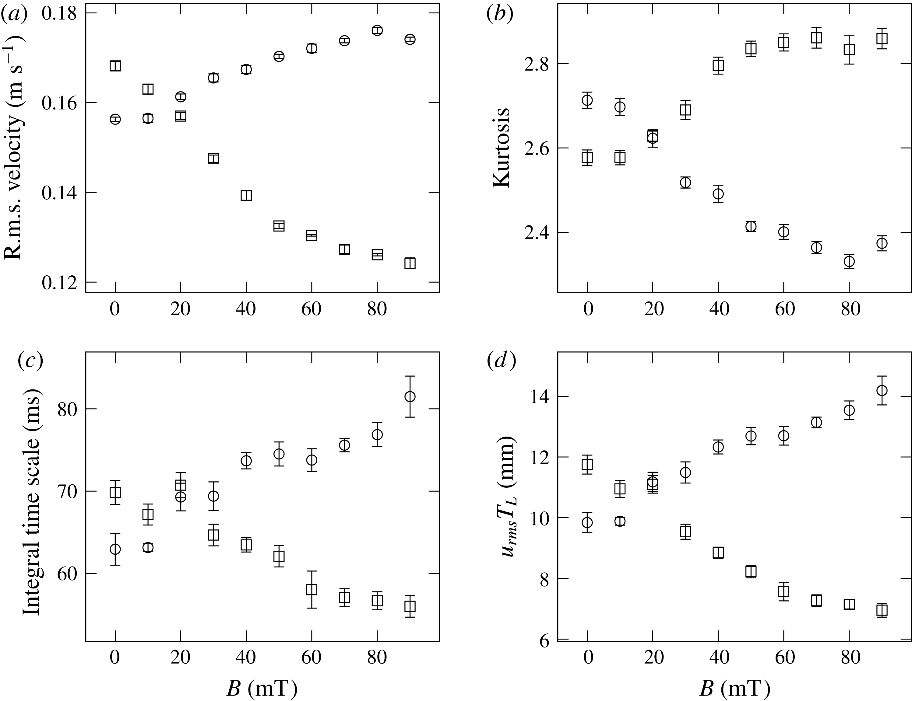
Statistics of transverse velocity components parallel (circles) and perpendicular (squares) to the magnetic field. (a) R.m.s. velocity, (b) velocity kurtosis, (c) integral time scale, and (d) product of r.m.s. velocity and integral time scale.

4.2 Large scales: velocity statistics

To begin the analysis of the Lagrangian time series data we look at the influence of the magnetic field on various large-scale quantities. Figure 11(a) shows the transverse velocity fluctuations in dependence on the magnetic field magnitude. Clearly there is an anisotropy in the r.m.s. velocities evolving with the magnetic field. The velocity kurtosis changes as well (figure 11 b) and confirms the change in the large-scale structure of the flow.

With increasing magnetic field, the flow in the field direction is much longer correlated than in the perpendicular to it (figure 11 c). Similar behaviour was reported by Shen & Yeung (Reference Shen and Yeung1997) in shear turbulence of fluid particles. The shape of the underlying autocorrelation remains similar – when normalised by the integral time scale all curves collapse for long time lags (not shown).

The product of r.m.s. velocity and integral time scale $u_{rms}T_{L}$ has the dimension of a length and can be considered as an integral length scale of the flow. For the isotropic case we found this length scale to be of order 10 mm independent of Reynolds number. With applied magnetic field it appears that eddies are compressed in the direction of the magnetic field (figure 11 d).

From the stochastic approach of Sawford (Reference Sawford1991) it follows that the Lagrangian time microscale ${\it\tau}_{{\it\lambda}}$ is given as

(4.1) $$\begin{eqnarray}{\it\tau}_{{\it\lambda}}\sim (T_{L}T_{2})^{1/2}.\end{eqnarray}$$

We test if this also holds for the anisotropic case. Figure 12 shows the ratio of ${\it\tau}_{{\it\lambda}}$ and $(T_{L}T_{2})^{1/2}$ as a function of the applied magnetic field. Taking into account the measurement uncertainty no clear trend is observable.

Figure 12.

Taylor time scale ${\it\tau}_{{\it\lambda}}$ normalised by $(T_{L}T_{2})^{1/2}$ against magnetic field for directions parallel (circles) and perpendicular (squares).

4.3 Inertial range: velocity differences

We may also evaluate the second-order structure functions of velocity components in the direction of the magnetic field $D_{2}({\it\tau})^{\Vert }$ and perpendicular to it $D_{2}({\it\tau})^{\bot }$ . Figure 13 shows the ratio $D_{2}({\it\tau})^{\Vert }/D_{2}({\it\tau})^{\bot }$ as a measure for anisotropy with time lag ${\it\tau}$ for several magnetic field magnitudes. At zero field there is the already mentioned small residual anisotropy that reduces at smaller scales. From the plot we conclude that (i) the anisotropy is greater at larger scales, and (ii) more pronounced at higher magnetic fields.

Figure 13.

Ratio of Lagrangian second-order structure functions against time lag. $T_{vis}$ is an estimate of the Kolmogorov microscale time scale for an external magnetic field magnitude of 70 mT.

Figure 14.

Velocity–acceleration covariance against magnetic field magnitude, (a) diagonal components and (b) off-diagonal components.

4.4 Velocity–acceleration covariance

We conclude our analysis by looking at the diagonal components of the velocity–acceleration covariance tensor, whose sum we use as an estimate of the energy dissipation rate in the flow (figure 14). While the axial component remains independent of magnetic field, the transverse components diverge symmetrically with increasing anisotropy. The transverse component perpendicular to the field $\langle u_{2}a_{2}\rangle$ also approaches the value of the axial component. This behaviour reflects the change of the flow topology which was seen in the Eulerian mean flow measurements.

The off-diagonal components in axial direction vanish (figure 14 b) while the off-diagonal components in the central plane are non-zero. They peak at a field around 20–30 mT and then return to the zero magnetic field values.