1 Introduction
The flow visualization of turbulent boundary layers realized by Kline et al. (Reference Kline, Reynolds, Schraub and Runstadler1967) revealed intermittent structures in the layers closest to the wall. The near-wall region is composed of alternating spanwise streaks of lower- and higher-speed fluid, with fairly regular spanwise spacing of approximately 100 wall units and amplitudes amounting to
 $\pm 50\,\%$
of the mean velocity. Streaks are closely related to the existence of streamwise counter-rotating vortices which alternately transport high-speed fluid towards the wall and low-speed fluid away from it. Wallace, Eckelmann & Brodkey (Reference Wallace, Eckelmann and Brodkey1972) introduced the quadrant classification of the plane of streamwise (
 $u$
) and wall-normal (
 $v$
) velocity fluctuations. The instantaneous product
 $uv$
was classified according to the sign of its components into four categories. They associated an upstream upwards motion (
 $u<0$
,
 $v>0$
, Q2 event) with the ejection process and attributed the opposite combination (
 $u>0$
,
 $v<0$
, Q4 event) to a sweep-type motion. The two other types of motion, with positive product
 $uv$
, were found to account for the ‘excess’ stress produced by the first two categories, which gives contributions of opposite sign. These sweep and ejection events result in the transfer of wall-normal momentum and the production of turbulent kinetic energy. Moreover, the low-speed streaks do not stay at the wall but migrate outward as they move downstream and then suddenly burst into intense, small-scale fluctuations. Kim, Kline & Reynolds (Reference Kim, Kline and Reynolds1971) shown that a very high fraction of the total turbulence production occurs during these relatively short bursting times.
These pioneering works aimed at describing turbulence through coherent structures have fundamentally changed our understanding of wall turbulence. While statistical descriptions and models for wall turbulence fail to describe repeating patterns of organized motion, structural approaches (i.e. devoted to the study of their geometries, characteristic length, temporal scales and convection velocities) offered a promising route for exploring their dynamics (Robinson Reference Robinson1991; Jiménez Reference Jiménez2018). In particular, since these coherent motions are seen to be responsible for the maintenance of turbulence in wall-bounded flows, their study has motivated a number of researches based on dynamical systems theory in the past couple of decades.
The fact that near-wall structures almost scale in inner units, namely with the kinematic viscosity and wall shear stress, indicates that they are universal features of wall-bounded flows. Jiménez & Moin (Reference Jiménez and Moin1991) used the possibilities of numerical simulations to investigate the origin of streaks. By reducing the streamwise and spanwise dimensions of the periodic domain, they could identify the dimensions of a minimal flow unit (MFU) below which turbulence could not be sustained. In addition, Jiménez & Pinelli (Reference Jiménez and Pinelli1999) further demonstrated that the dynamics at the MFU is autonomous, the self-sustaining mechanism being independent of the peculiar outer flow. In this vein, Hamilton, Kim & Waleffe (Reference Hamilton, Kim and Waleffe1995) developed the self-sustaining process (SSP) at play in wall-bounded turbulent flows (see Panton (Reference Panton2001) for a review). The authors established three fundamental elements: (i) rolls distribute streamwise velocity through the linear non-modal lift-up effect (Landhal Reference Landhal1980) to generate streaks; (ii) fluctuations will in turn become amplified due to the secondary instability of streaks; and (iii) nonlinear quadratic interactions of instability waves regenerate rolls. Waleffe (Reference Waleffe1998, Reference Waleffe2003) further confirmed the validity of the SSP theory by computing three-dimensional invariant states (steady or travelling waves) in plane Couette and channel flows using a continuation method. Since then, this theory has been applied with success to describe equilibrium states where streamwise vortices, streaks and neutral eigenmodes combine to reach a sustained travelling wave equilibrium (Kawahara, Uhlmann & Veen Reference Kawahara, Uhlmann and Veen2012). For wall-bounded flow, these equilibria produce a state space representation that shows the role of coherent states and their unstable manifolds in guiding turbulent dynamics (Gibson, Halcrow & Cvitanovic Reference Gibson, Halcrow and Cvitanovic2008). Continuation revealed that these equilibrium states arise from a saddle-node bifurcation for various wall-bounded flows (Couette and channel flows, for instance) at some Reynolds number for a given computational box. Two solutions are found to emerge at the critical Reynolds number: one associated with a lower-branch solution that is characterized by a low skin friction drag, and an upper-branch solution that has a high drag. Waleffe (Reference Waleffe2003) and many others since then have shown that, while the lower-branch solution is associated with a separatrix between the laminar and turbulent attractors (where one unstable direction is identified), the upper-branch solutions are shown to match reasonably well with wall turbulence at low Reynolds numbers (in terms of both statistics and coherent structures). This result gave strong support that states lying on the upper branch represent saddle points in the phase space of the turbulent attractor. Such invariant structures are thus referenced as exact coherent states (ECSs) by previous authors. These analyses were recently extended to high Reynolds numbers using the filtered Navier–Stokes equations by Cossu and co-workers (see Cossu & Hwang (Reference Cossu and Hwang2017) for a review).
Recent studies have supported that wall turbulence exhibits different states in its dynamics. While strong turbulence activity dominates for long periods of time, weak turbulence, as evidenced by a drag reduction, occurs for short time intervals. During recent decades, new numerical tools have been dedicated to the computation of rare events by selecting trajectories (see Tailleur & Kurchan (Reference Tailleur and Kurchan2007) and Ragone, Wouters & Bouchet (Reference Ragone, Wouters and Bouchet2017), among others). Given the complexity of turbulence, direct application of these methods to Navier–Stokes equations is impracticable; therefore, it appears necessary to consider some simplified models.
In that respect, Park & Graham (Reference Park and Graham2015) found a new family of travelling wave solutions that emerge through a saddle-node bifurcation for the case of channel flow. In particular, the authors have shown that, while statistics carried out on the upper-branch solution (i.e. associated with the higher friction velocity) strongly match with turbulent channel flow profiles, the lower-branch solution (i.e. associated with the lower friction velocity) exhibits a mean flow profile that approaches the Virk log law (Virk, Mickley & Smith Reference Virk, Mickley and Smith1970). It is widely accepted that mean velocity profiles most closely approach this law in the log region of a channel flow with homogeneous additive polymer; it has only recently been shown that this state defines a universal limit for Newtonian turbulence, the so-called maximum drag reduction (MDR) asymptote (see Xi & Bai (Reference Xi and Bai2016) for a recent review).
More recently, Kushwaha, Park & Graham (Reference Kushwaha, Park and Graham2017) have shown that, for low Reynolds numbers, turbulence in channel flow exhibits intermittency that is closely tied to chaotic movement of turbulence trajectories between the lower- and upper-branch solutions found by Park & Graham (Reference Park and Graham2015). By using a shooting method, Itano & Toh (Reference Itano and Toh2001) and Toh & Itano (Reference Toh and Itano2003) have tracked ECSs for a channel flow within a minimal flow framework. This solution consists of a periodic-like solution localized on one side of the channel in the wall-normal direction. One cycle of the ECS is characterized by two different motions. While, for a very long quiescent phase, the flow state exhibits a single streak, the latter is shifted in the spanwise direction after each bursting event where the flow structure is dominated by a double-streak motion. Because previous authors only succeeded to track the solution for one-and-a-half periods, no definitive statement has been made whether the solution converges on a heteroclinic cycle or a periodic orbit. Recently, Zammert & Eckhardt (Reference Zammert and Eckhardt2014) and Rinaldi, Schlatter & Bagheri (Reference Rinaldi, Schlatter and Bagheri2018) revisited this previous solution. Using the same shooting method, they were able to track the ECS on several cycles alternating between burst and long quiet intervals. On the one hand, the latter analysis gave thus a strong indication that the finite-amplitude solution is attracted to a period orbit. On the other hand, they show that, for wider domains, the attracting state is localized in the spanwise direction. Similarly, in the asymptotic suction flat-plate boundary layer, Kreilos et al. (Reference Kreilos, Veble, Schneider and Eckhardt2013) also found an ECS that exhibits the same dynamical activity, providing further evidence that such a periodic state is a universal feature of wall-bounded flow. Hence, it may also be suggested that such periodic solutions can be representative of turbulent trajectories between low- and high-drag events.
In order to reduce the complexity of the dynamics, important expectations emerged from the linear analysis. The only mathematical justification for the linear assumption of non-infinitesimal fluctuations is provided by the rapid distortion theory (RDT). This theory goes back to a paper of Taylor (Reference Taylor1935), who analysed the damping of turbulent fluctuations in flow through a contraction in a wind tunnel. If the straining is sufficiently rapid, then its effect on the turbulence may be treated in a first approximation by a linearized analysis. The nonlinear interaction of the turbulence with itself is neglected. The distinction between the terms ‘rapid’ (linear) and ‘slow’ (nonlinear) is derived from the fact that only the rapid part responds immediately to a change imposed on the mean field, and the slow part will feel the change through nonlinear interactions. For further details and the various applications, see the overview by Hunt & Carruthers (Reference Hunt and Carruthers1990). By solving the instantaneous linear equations of the RDT, Lee & Moin (Reference Lee and Moin1990) have shown that a high shear rate produces structures in homogeneous turbulence similar to the streaks observed in the sublayer of wall-bounded turbulent shear flows. That numerical result has been experimentally confirmed by Diwan & Morrison (Reference Diwan and Morrison2017).
A heuristic argument for the linear dynamics of fluctuations around a nonlinear mean flow was proposed by Malkus (Reference Malkus1956). He conjectured that the turbulent mean state is in equilibrium with the turbulent perturbations responsible for the Reynolds stresses, the perturbations being in the subspace of the neutral modes of the linearized Navier–Stokes equations. Malkus tested this promising idea with a time-averaged flow but failed to obtain a neutral mode. Renewed interest followed the new findings about subcritical transition to turbulence of linearly stable wall flows. Butler & Farrell (Reference Butler and Farrell1993) applied an optimization method to compute the most amplified streaks over an appropriate turbulent eddy turnover time, and the streak spacing was found to be in good agreement with the expected value, approximately 100 wall units. Similarly, linear models based on the resolvent analysis technique proposed by Hwang & Cossu (Reference Hwang and Cossu2010) and McKeon & Sharma (Reference McKeon and Sharma2010) and further explored by Sharma & McKeon (Reference Sharma and McKeon2013) and Sharma, Moarref & McKeon (Reference Sharma, Moarref and McKeon2017) have also clearly enlightened the relevance of the linear mechanism to build a modelling framework for wall-turbulent coherent motions. Nevertheless, these linear studies failed to describe the SSP and intermittency or bursts.
All these studies used a time-averaged mean flow, extracted from direct numerical simulation (DNS), for example, so the mean flow is decoupled from the fluctuations. In fact, the time averaging is too restrictive and Farrell & Ioannou (Reference Farrell and Ioannou1996) argued that non-stationarity is a fundamental ingredient in turning transient growth into sustained growth. The growth of short scales forces the temporal oscillation of long scales, and the non-stationarity of the latter continuously restarts the transient growth. Equilibrium is more a cycle rather than a permanent balance between energy production and dissipation.
An attractive variation is the division of the flow into infinitely long streaks and vortices and the corresponding fluctuation. The streaks are nonlinear and driven by vortices which are generated by nonlinear Reynolds stresses created by small scales. These scales evolve within the non-uniform flow field of the streak, but all nonlinear interactions among themselves are neglected. That restricted nonlinear (RNL) model is two-dimensional in the cross-flow plane with three velocity components; it permits a reduction of the numerical cost and a simplification of the dynamics. Despite its simplicity, that reduction is able to reproduce the essential features of transitional and turbulent flows.
Biau & Bottaro (Reference Biau and Bottaro2009) used the RNL system associated with an optimization method to follow an optimal path to transition in a linearly stable duct flow. The model was able to reach a sustained turbulence. A parametric study on the single streamwise wavelength of the fluctuation shows a cut-off of approximately 300 wall units, below which no transition can be observed, which corresponds to the minimal flow unit obtained with DNS. Moreover, the optimal solution from the RNL system is close to the nonlinear solution sited on the laminar–turbulent separatrix, sometimes called the edge state.
Farrell & Ioannou (Reference Farrell and Ioannou2012) used the RNL system with a stochastic forcing (see also the overview in Farrell, Gayme & Ioannou (Reference Farrell, Gayme and Ioannou2017)). Their results confirmed that this RNL system supports a realistic SSP. At small forcing amplitudes, the only stable equilibrium of the model system is laminar, but, as the forcing increases, there is first a bifurcation from laminar state to steady streaks and rolls, and later another one to an unsteady ‘bursting’ state. Bretheim, Meneveau & Gayme (Reference Bretheim, Meneveau and Gayme2015) have shown that simulations using the RNL system with appropriately chosen streamwise modes, namely the band-limited RNL model, exhibit the main characteristics of wall turbulence, similar coherent motions and statistics even if only a few streamwise Fourier wavenumbers are retained. In particular, mean velocity profiles obtained with such a band-limited RNL model follow the standard logarithmic law. An RNL model was also introduced by Willis & Kerswell (Reference Willis and Kerswell2009) for localized turbulence in pipe flow. For this purpose, the mean flow is axisymmetric with one Fourier mode in azimuth which is able to reproduce the observed behaviour such as localized ‘puff’ structures and ‘slug’ turbulence.
While previous studies have proven fruitful in gaining a better understanding of RNL systems applied to sustained turbulence, the scope of this paper is to extend these approaches by capturing invariant solutions that aim to describe the closed path along turbulent saddle points and intermittency within an RNL framework. For that purpose, the present study is devoted to investigate the exact coherent periodic state initially found by Toh & Itano (Reference Toh and Itano2003) using DNS with RNL simulations where only a single Fourier mode in the streamwise direction is retained. In particular, we will investigate whether or not this minimal representation of flow dynamics is able to capture the essential features of the cycle, such as bursting events, spanwise shifts, long quiescent phases or high- and low-drag events. For that purpose, both flow structures and statistics will be investigated. The paper will be organized as follows. After having presented governing equations and numerical methods in § 2, the tracked solution computed using an RNL system is discussed in the light of previous studies and statistics provided by DNS database in § 3. In particular, the connection between bursting events and near-wall turbulence will be investigated. The influence of spanwise width, Reynolds number and streamwise wavenumber onto the edge-tracked solution will be discussed in § 4. Finally, § 5 will be devoted to draw some conclusions and prospects.
2 Method
2.1 Governing equations
We consider the pressure-driven incompressible flow of a Newtonian fluid in a plane channel maintained at constant mass flux. The usual set of Cartesian coordinates
 $(x,y,z)$
and velocity components
 $\boldsymbol{u}=(u,v,w)$
are adopted in the streamwise, wall-normal and spanwise directions, respectively. The half-channel height
 $h$
is chosen as the characteristic length scale, and velocities are scaled with the laminar centreline velocity
 $U_{c}$
for the given mass flux. The corresponding Reynolds number is defined as
 $Re=U_{c}h/\unicode[STIX]{x1D708}$
, with
 $\unicode[STIX]{x1D708}$
the kinematic viscosity. In the following, the selected value is
 $Re=U_{c}h/\unicode[STIX]{x1D708}=3000$
, as used in Itano & Toh (Reference Itano and Toh2001) and Toh & Itano (Reference Toh and Itano2003), and corresponds to a value
 $Re_{b}=2000$
based on the bulk velocity.
The non-dimensional Navier–Stokes equations are then given by
 $$\begin{eqnarray}\left.\begin{array}{@{}c@{}}\displaystyle \frac{\unicode[STIX]{x2202}\boldsymbol{u}}{\unicode[STIX]{x2202}t}+\boldsymbol{u}\boldsymbol{\cdot }\unicode[STIX]{x1D735}\boldsymbol{u}=-G(t)\boldsymbol{e}_{\boldsymbol{x}}-\unicode[STIX]{x1D735}p+\frac{1}{Re}\unicode[STIX]{x1D6FB}^{2}\boldsymbol{u},\\ \displaystyle \unicode[STIX]{x1D735}\boldsymbol{\cdot }\boldsymbol{u}=0,\end{array}\!\right\}\end{eqnarray}$$
where
 $\boldsymbol{e}_{\boldsymbol{x}}=(1,0,0)$
. The uniform pressure gradient,
 $G(t)$
, that drives the flow is adjusted dynamically to maintain a constant mass flux. No-slip boundary conditions are applied on the two walls
 $y=\pm 1$
and periodic boundary conditions are adopted in the homogeneous streamwise and spanwise directions. Hereafter, we denote
 $u_{\unicode[STIX]{x1D70F}}$
the friction velocity and quantities in inner scaling are referenced with the
 $+$
superscript. The friction Reynolds number is denoted
 $Re_{\unicode[STIX]{x1D70F}}=u_{\unicode[STIX]{x1D70F}}h/\unicode[STIX]{x1D708}$
.
In the present work, the quasi-linear restriction of the dynamics to roll–streak interactions, namely the so-called RNL system (Farrell et al.
Reference Farrell, Ioannou, Jiménez, Constantinou, Lozano-Durán and Nikolaidis2016), is used to study finite-amplitude solutions of plane channel flow. In this context, the velocity
 $\boldsymbol{u}$
is decomposed into mean and perturbation components:
 $$\begin{eqnarray}\boldsymbol{u}=\boldsymbol{U}+\boldsymbol{u}^{\prime }.\end{eqnarray}$$
The mean velocity is
 $\boldsymbol{U}(y,z,t)=\langle \boldsymbol{u}\rangle$
with
 $\langle ~\rangle$
the averaging operator in the streamwise direction. An overbar over any quantities will denote averaging along the spanwise direction. The pressure is similarly split into
 $p(x,y,z,t)=G(t)x+P(y,z,t)+p^{\prime }(x,y,z,t)$
.
The fluctuation can be decomposed into a Fourier expansion. Hereafter, we will consider a minimal RNL system where only a single streamwise component is retained. The fluctuations are thus expressed as
 $$\begin{eqnarray}\boldsymbol{u}^{\prime }=\hat{\boldsymbol{u}}\text{e}^{\text{i}\unicode[STIX]{x1D6FC}x}+\hat{\boldsymbol{u}}^{\ast }\text{e}^{-\text{i}\unicode[STIX]{x1D6FC}x},\end{eqnarray}$$
with
 $\unicode[STIX]{x1D6FC}$
the streamwise wavenumber. As a consequence, the nonlinear terms in the fluctuation equation
 $\boldsymbol{u}^{\prime }\boldsymbol{\cdot }\unicode[STIX]{x1D735}\boldsymbol{u}^{\prime }-\langle \boldsymbol{u}^{\prime }\boldsymbol{\cdot }\unicode[STIX]{x1D735}\boldsymbol{u}^{\prime }\rangle$
only contain first harmonics, namely modes with wavenumbers
 $\pm 2\unicode[STIX]{x1D6FC}$
; hence they are neglected with the single-mode restriction. The RNL model is thus derived from the Navier–Stokes equations through a Galerkin truncation procedure similar to that used to derive the Lorenz model of Rayleigh–Bénard convection. Attention must be paid to this severe truncation; indeed Curry et al. (Reference Curry, Herring, Loncaric and Orszag1984) found that the chaos observed in the Lorenz system is in fact a product of inadequate spatial resolution. The RNL model is minimal in the sense that it assumes a separation of scales that does not exist in reality, so the model does not really represent multiscale turbulence. Another issue concerns the dependence of the nonlinear mean flow with respect to the streamwise length of the computational domain. On the other hand, the model is deterministic and rigorously derived from the Navier–Stokes equations.
As stated by Waleffe & Kim (Reference Waleffe, Kim and Panton1997) and Biau & Bottaro (Reference Biau and Bottaro2009), the model may be further simplified by considering that
 $\boldsymbol{u}^{\prime }$
is of order
 $O(\unicode[STIX]{x1D700})$
. The roll vortices
 $V$
and
 $W$
are of order
 $O(\unicode[STIX]{x1D700}^{2})$
and the streak component of the streamwise mean flow
 $U$
is of order
 $O(\unicode[STIX]{x1D700}^{2}Re)$
as a consequence of the lift-up mechanism (Schmid & Henningson Reference Schmid and Henningson2001). This approximation is consistent with the results given by Wang, Gibson & Waleffe (Reference Wang, Gibson and Waleffe2007), who have shown that the travelling wave solution, associated with the lower branch, scales with Reynolds number
 $Re$
such that streaks are of order one but rolls are
 $O(Re^{-1})$
, the fundamental fluctuating mode scales with
 $O(Re^{-1})$
while the harmonics are
 $o(Re^{-1})$
. Hence, at the order
 $O(Re^{-1})$
, the dynamics of ECS lying on the lower branch is consistent with the RNL system. More recently, Hall & Sherwin (Reference Hall and Sherwin2010) and Blackburn, Hall & Sherwin (Reference Blackburn, Hall and Sherwin2013) have developed a similar analysis to compute three-dimensional rolls–perturbation interaction equilibria of laminar plane Couette flow for high-Reynolds-number flow cases.
Nonetheless, the issue of capturing travelling wave characteristics of the upper branch and more complex solutions such as periodic states suffer from a lack of rigorous justification. However, for low Reynolds numbers, Pausch et al. (Reference Pausch, Yang, Hwang and Eckhardt2018) have recently shown that travelling wave states associated with the upper-branch solution for both plane channel flows and Couette flows are still well approximated using assumptions that hold for lower-branch solutions.
The equations governing the mean, streamwise-averaged flow read
 $$\begin{eqnarray}\left.\begin{array}{@{}c@{}}\displaystyle V_{y}+W_{z}=0,\\ \displaystyle U_{t}+VU_{y}+WU_{z}=-G(t)+Re^{-1}(U_{yy}+U_{zz})-\unicode[STIX]{x2202}_{y}(\hat{v}^{\ast }\hat{u} +\hat{v}\hat{u} ^{\ast })-\unicode[STIX]{x2202}_{z}({\hat{w}}^{\ast }\hat{u} +{\hat{w}}\hat{u} ^{\ast }),\\ \displaystyle V_{t}=-P_{y}+Re^{-1}(V_{yy}+V_{zz})-\unicode[STIX]{x2202}_{y}(2\hat{v}\hat{v}^{\ast })-\unicode[STIX]{x2202}_{z}({\hat{w}}^{\ast }\hat{v}+{\hat{w}}\hat{v}^{\ast }),\\ \displaystyle W_{t}=-P_{z}+Re^{-1}(W_{yy}+W_{zz})-\unicode[STIX]{x2202}_{y}(\hat{v}^{\ast }{\hat{w}}+\hat{v}{\hat{w}}^{\ast })-\unicode[STIX]{x2202}_{z}(2{\hat{w}}^{\ast }w),\end{array}\right\}\end{eqnarray}$$
associated with homogeneous boundary conditions
 $U=V=W=0$
on the walls. The streamwise pressure gradient
 $G(t)$
is adjusted to fix the mass flow rate. The Navier–Stokes equations, linearized around the streaky flow, are
 $$\begin{eqnarray}\left.\begin{array}{@{}c@{}}\displaystyle \text{i}\unicode[STIX]{x1D6FC}\hat{u} +\hat{v}_{y}+{\hat{w}}_{z}=0,\\ \displaystyle \hat{u} _{t}+\text{i}\unicode[STIX]{x1D6FC}U\hat{u} +\hat{v}U_{y}+{\hat{w}}U_{z}=-\text{i}\unicode[STIX]{x1D6FC}\hat{p}+Re^{-1}(-\unicode[STIX]{x1D6FC}^{2}\hat{u} +\hat{u} _{yy}+\hat{u} _{zz}),\\ \displaystyle \hat{v}_{t}+\text{i}\unicode[STIX]{x1D6FC}U\hat{v}=-\hat{p}_{y}+Re^{-1}(-\unicode[STIX]{x1D6FC}^{2}\hat{v}+\hat{v}_{yy}+\hat{v}_{zz}),\\ \displaystyle {\hat{w}}_{t}+\text{i}\unicode[STIX]{x1D6FC}U{\hat{w}}=-\hat{p}_{z}+Re^{-1}(-\unicode[STIX]{x1D6FC}^{2}{\hat{w}}+{\hat{w}}_{yy}+{\hat{w}}_{zz}),\end{array}\right\}\end{eqnarray}$$
together with
 $\hat{u} =\hat{v}={\hat{w}}=0$
on the walls.
In the present configuration, the system (2.4) and (2.5) is capable of yielding a self-sustained state based on linear growth of
 $\boldsymbol{u}^{\prime }$
, generation of streamwise vortices due to the fluctuation Reynolds stress forcing, production of streaks by lift-up effect and regeneration of
 $U$
.
2.2 Exact coherent state trajectory
There is typically a parameter in front of the stresses that feed back into the streaks and vortices, equivalent to the amplitude of the fluctuations, that has to be adjusted to prevent secular terms. To constrain a phase-space trajectory to stay on the edge surface, a shooting method as first described by Itano & Toh (Reference Itano and Toh2001) and Toh & Itano (Reference Toh and Itano2003) is used by considering the coupled system of equations (2.4) and (2.5). To obtain a finite-amplitude solution, Toh & Itano (Reference Toh and Itano2003) suggest the introduction of a similar decomposition to the one associated with the RNL system: a quasi-two-dimensional state and three-dimensional fluctuation. By using DNS, the latter authors search for a solution lying on the edge by adjusting the shooting parameter at an initial time. The procedure is then repeated for adjacent time intervals. This shooting method is well suited to track a dynamical trajectory that exhibits heteroclinic connections (Duguet, Willis & Kerswell Reference Duguet, Willis and Kerswell2008; Schneider et al.
Reference Schneider, Gisbon, Lagha, Lillo and Eckhardt2008). It further indicates the ability of this approach to deal with the periodic solution found by Toh & Itano (Reference Toh and Itano2003). When considering an RNL system, the shooting method is straightforward. Let us introduce a shooting parameter
 $f_{i}$
such that
 $$\begin{eqnarray}\boldsymbol{u}_{i}=\boldsymbol{U}_{i}+f_{i}\boldsymbol{u}_{i}^{\prime },\end{eqnarray}$$
where the subscript
 $i$
denotes the time interval. The fitting parameter
 $f_{i}$
is adjusted such that the amplitude of the fluctuation
 $\boldsymbol{u}^{\prime }$
is kept finite in the time interval
 $i$
. Unlike previous studies based on DNS, both the mean flow and fluctuation are already provided by the RNL system. The inherent difficulty to track the edge for a long time interval due to double-precision limitation is overcome by computing a distinct shooting parameter for each time substep. Hereafter, using a bisection method,
 $f_{i}$
is refined up to
 $14$
significant digits in double precision for a given dimensionless time interval
 $t_{i}+\unicode[STIX]{x1D6FF}t$
, where
 $t_{i}$
is fixed at
 ${\approx}350$
and
 $\unicode[STIX]{x1D6FF}t\approx 2t_{i}$
.
2.3 Numerical methods
The numerical method is based on a spectral approximation of the velocity fields using Fourier expansions in both the streamwise and spanwise directions and Chebyshev polynomials in the wall-normal direction. The divergence-free condition is achieved by using the Uzawa method (Peyret Reference Peyret2002). The discrete system attached to (2.4) and (2.5) is solved at each time step using a semi-implicit second-order extrapolation/backward differentiation scheme as described by Peyret (Reference Peyret2002). In particular, convective terms are treated explicitly while an implicit scheme is used for viscous terms. For dealiasing, the
 $3/2$
rule is adopted for Fourier expansions. The numerical method is further detailed in Alizard (Reference Alizard2015) and a validation of the code is carried out in Alizard (Reference Alizard2017). For the RNL model, the domain sizes are first identical to those used by Toh & Itano (Reference Toh and Itano2003):
 $\unicode[STIX]{x03C0}$
, 2 and
 $0.4\unicode[STIX]{x03C0}$
with
 $1\times 80\times 32$
grid points. This gives a streamwise wavenumber
 $\unicode[STIX]{x1D6FC}=2$
. For the DNS, a similar spectral method is used; and the domain sizes are six times larger,
 $6\unicode[STIX]{x03C0}$
, 2 and
 $2.4\unicode[STIX]{x03C0}$
with
 $256\times 151\times 256$
grid points, respectively, in streamwise, wall-normal and spanwise directions. The grid spacings in the streamwise and spanwise directions are respectively
 $\unicode[STIX]{x0394}x^{+}=9.8$
and
 $\unicode[STIX]{x0394}z^{+}=3.9$
in wall units.
3 Results
3.1 Direct numerical simulation
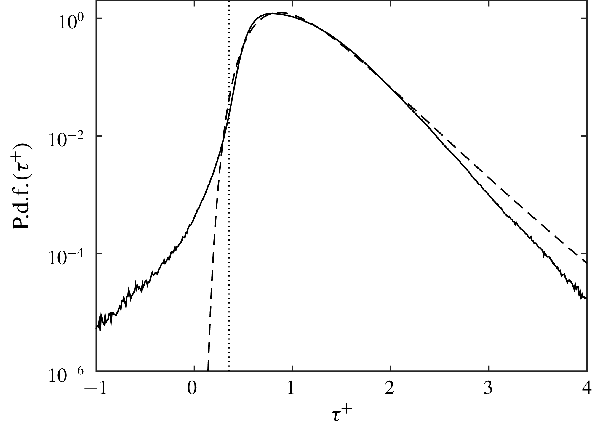
As a preliminary result, figure 1 shows the probability distribution (density) function (p.d.f.) of the wall shear stress fluctuations
 $\unicode[STIX]{x1D70F}$
normalized with its mean value
 $2\times 10^{-3}$
. The viscous scaling provides a good collapse, except for the tails (Örlü & Schlatter Reference Örlü and Schlatter2011). The p.d.f. is well described by a log-normal distribution, as first shown by Alfredsson, Örlü & Schlatter (Reference Alfredsson, Örlü and Schlatter2011), given by
 $$\begin{eqnarray}f(\unicode[STIX]{x1D70F})=\frac{1}{\unicode[STIX]{x1D70E}\sqrt{2\unicode[STIX]{x03C0}}}\text{e}^{-(\ln \unicode[STIX]{x1D70F}-\unicode[STIX]{x1D707})^{2}/(2\unicode[STIX]{x1D70E}^{2})},\end{eqnarray}$$
with
 $\unicode[STIX]{x1D707}=-0.0278$
and
 $\unicode[STIX]{x1D70E}=0.3447$
, respectively, the mean and root-mean-square (r.m.s.) values of
 $\ln \unicode[STIX]{x1D70F}$
. Log-normal variability is basically based on a variety of forces acting independently with multiplicative effects which are encountered in many fields of physics (Limpert, Stahel & Abbt Reference Limpert, Stahel and Abbt2001). Log-normal distributions have also been found to describe various phenomena in near-wall turbulence, e.g. the average inner normalized streak spacing (Smith & Metzler Reference Smith and Metzler1983), and the time interval between burst events (Rao, Narasimha & Narayanan Reference Rao, Narasimha and Narayanan1971).
Probability distribution function of the streamwise wall shear stress normalized with the mean value. The p.d.f. is compared to a log-normal distribution (dashed line). The laminar value is indicated with the vertical dotted line.

The p.d.f. of the wall shear stress (figure 1) shows the existence of high- and low-drag events; interestingly, the probability to observe a sublaminar drag is approximately 0.17 %.
3.2 Periodic solution of minimal restricted nonlinear model
In this section, the periodic solution studied by Toh & Itano (Reference Toh and Itano2003) and Zammert & Eckhardt (Reference Zammert and Eckhardt2014) is revisited using the minimal RNL system. The same initial conditions as given by Toh & Itano (Reference Toh and Itano2003) are used for the system (2.4) and (2.5):
 $$\begin{eqnarray}\boldsymbol{U}=\left(1-y^{2},-\frac{\unicode[STIX]{x2202}\unicode[STIX]{x1D6F9}}{\unicode[STIX]{x2202}z},\frac{\unicode[STIX]{x2202}\unicode[STIX]{x1D6F9}}{\unicode[STIX]{x2202}y}\right),\quad \displaystyle \boldsymbol{u}^{\prime }=\left(0,0,-\frac{\unicode[STIX]{x2202}\unicode[STIX]{x1D6F7}}{\unicode[STIX]{x2202}y}\right),\end{eqnarray}$$
where
 $\unicode[STIX]{x1D6F9}(y,z)=F(y)\sin (2\unicode[STIX]{x03C0}z/L_{z})$
,
 $\unicode[STIX]{x1D6F7}(x,y)=F(y)\sin (2\unicode[STIX]{x03C0}x/L_{x})$
and
 $F(y)=A(\exp (c_{m}(-y-1))-1)^{2}(\exp (c_{p}(y-1))-1)^{2}$
, with
 $A=1\times 10^{-10}$
,
 $c_{m}=1$
and
 $c_{p}=-6$
. It consists of a pair of streamwise vortices located near the lower wall superimposed onto the Poiseuille flow solution. For a sufficiently high perturbation amplitude, a secondary instability occurs.
To describe the solution lying on the edge, we introduce the kinetic energy norm of the fluctuation:
 $$\begin{eqnarray}E=\int _{-1}^{1}\int _{-L_{z}/2}^{L_{z}/2}\hat{\boldsymbol{u}}\boldsymbol{\cdot }\hat{\boldsymbol{u}}^{\ast }\,\text{d}y\,\text{d}z.\end{eqnarray}$$
To characterize the number of streaks associated with the solution, we also define the kinetic energy norms for the fluctuation restricted to the fundamental and its first harmonic spanwise Fourier mode as
 $E_{1}$
and
 $E_{2}$
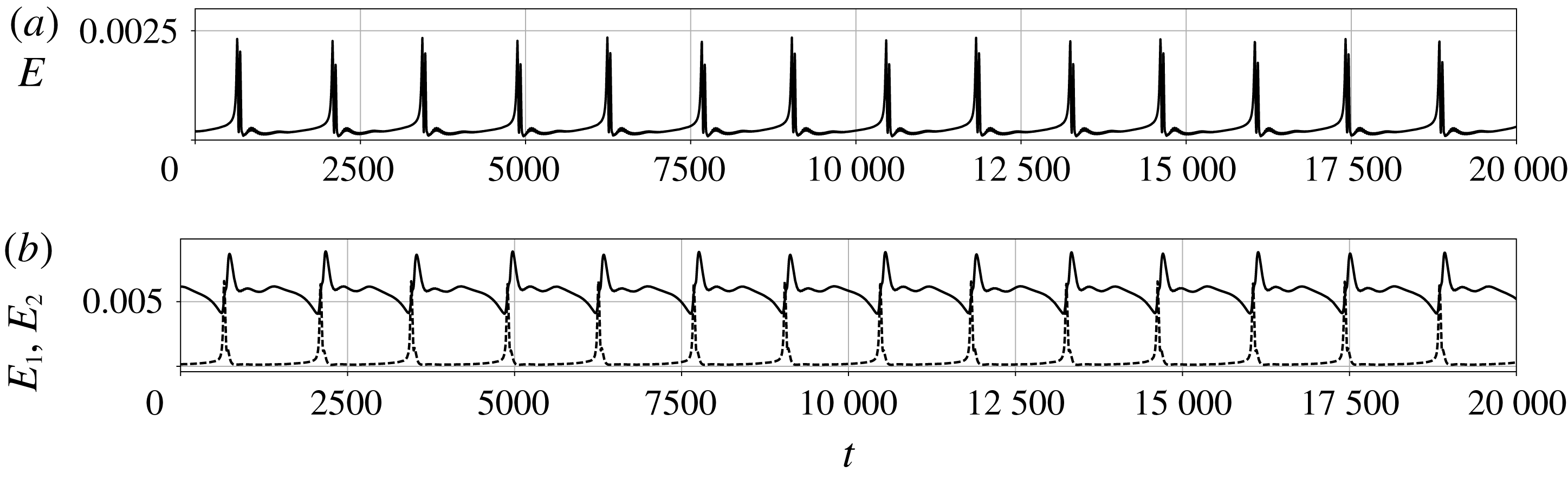
. In figure 2(a),
 $E(t)$
is shown. After a transient behaviour, the shooting parameter
 $f_{i}$
is found to oscillate between
 $0.992$
and
 $0.998$
. The fact that
 $f_{i}$
is close to one suggests that the solution obtained by connecting each time substep approximates reasonably well the exact solution. The trajectory resulting from the shooting method exhibits a convergence towards a simple state. The latter is characterized by long quiescent intervals separated by quick bursting events that repeat periodically, as shown in figure 2(a). Figure 2(b) displays the time evolution of
 $E_{1}$
and
 $E_{2}$
. The figure shows that, while the flow is dominated by one pattern along the spanwise direction during quiet phases, the bursting event is characterized by competition between the fundamental and its first harmonic spanwise Fourier mode.
Time evolution of (a) kinetic energy of the fluctuation and (b) kinetic energy of fluctuation restricted to the fundamental mode (full line) and the first harmonic (dashed line). The transient phase before convergence to the edge state is discarded.

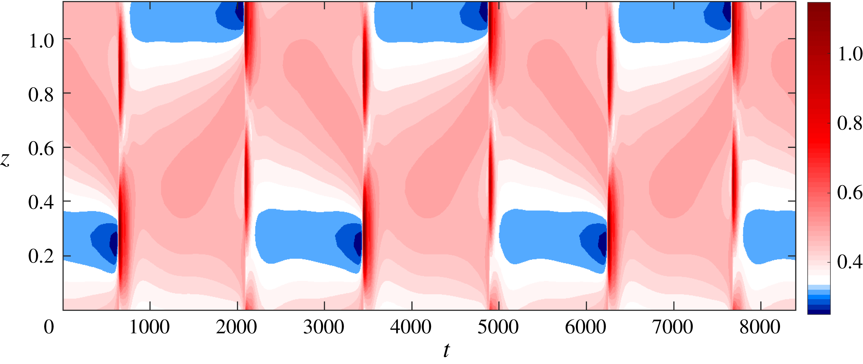
In figure 3, the wall shear stress distribution normalized with the turbulent value is shown in the plane
 $(t,z)$
for a time interval that includes several bursts. The figure shows that the burst is accompanied by a strong increase of wall skin friction where the latter reaches a level close to the turbulent one. It is also interesting to note that, while the wall shear stress has a slightly higher level than its laminar counterpart (i.e.
 ${\approx}0.35$
) during the major part of the quiescent phase, it also exhibits sublaminar drag events. This suggests that the minimal representation of this periodic solution is connected to close passes along the turbulent attractor which shares similarities with statistics shown in figure 1. The results are also consistent with Toh & Itano (Reference Toh and Itano2003), Zammert & Eckhardt (Reference Zammert and Eckhardt2014) and Rinaldi et al. (Reference Rinaldi, Schlatter and Bagheri2018).
Spanwise and time evolution of the wall shear stress, normalized with the turbulent value, associated with the periodic edge.

3.3 Equilibrium states and bursts
To further characterize the solution provided by the RNL restriction, we examine the evolution of the kinetic energy input rate
 ${\mathcal{I}}$
and the dissipation
 $\unicode[STIX]{x1D716}$
of the system
 $$\begin{eqnarray}\frac{\text{d}{\mathcal{E}}}{\text{d}t}={\mathcal{I}}-\unicode[STIX]{x1D716},\end{eqnarray}$$
with
 $$\begin{eqnarray}{\mathcal{I}}=-\int _{D}\frac{\text{d}p}{\text{d}x}\,\boldsymbol{u}\boldsymbol{\cdot }\boldsymbol{e}_{\boldsymbol{x}}\,\text{d}D\quad \text{and}\quad \unicode[STIX]{x1D716}=\frac{1}{Re}\int _{D}\unicode[STIX]{x1D735}\boldsymbol{u}\mathbf{: }\unicode[STIX]{x1D735}\boldsymbol{u}\,\text{d}D.\end{eqnarray}$$
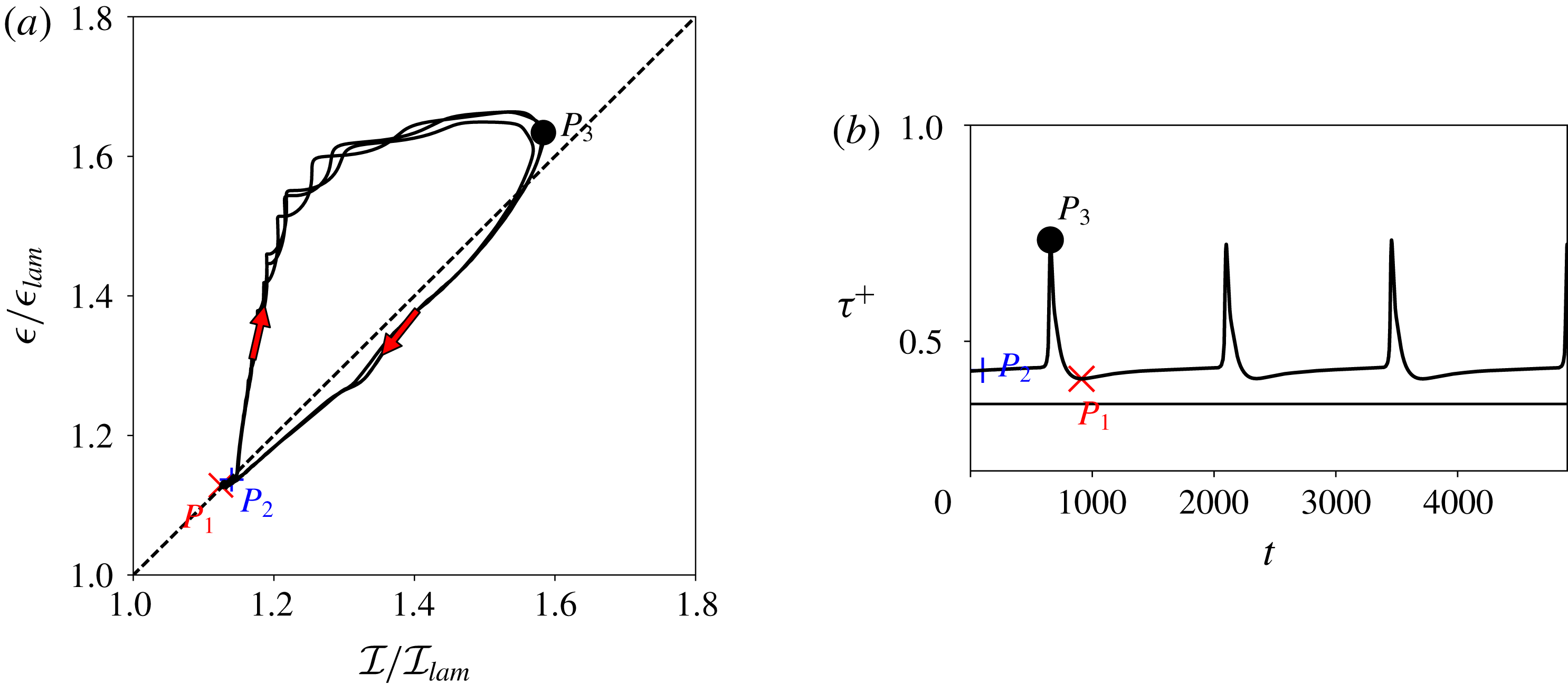
In figure 4(a,b), the energy input–dissipation rate trajectory and the corresponding time evolution of the wall shear stress for
 $\overline{U}$
(i.e. spanwise-averaged
 $U$
) are shown for the minimal RNL solution. Three characteristic points, referenced as
 $P_{1},~P_{2}$
and
 $P_{3}$
, are also depicted in figure 4(a,b). While the solution spends a relatively long time near
 $P_{1}$
and
 $P_{2}$
, it orbits only briefly along
 $P_{3}$
where the dissipation and
 $\unicode[STIX]{x1D70F}^{+}$
are maximum. One may note that
 $P_{1},~P_{2}$
and
 $P_{3}$
exhibit almost an equilibrium state where the production is balanced by the dissipation. The periodic solution trajectory obtained using the minimal RNL system bears a close resemblance to the one described by Toh & Itano (Reference Toh and Itano2003), in both amplitudes and excursions to saddle points. Nevertheless, while Toh & Itano (Reference Toh and Itano2003) pointed out that the phase portrait exhibits an almost equilibrium state for
 ${\mathcal{P}}/{\mathcal{P}}_{lam}\approx 1.25$
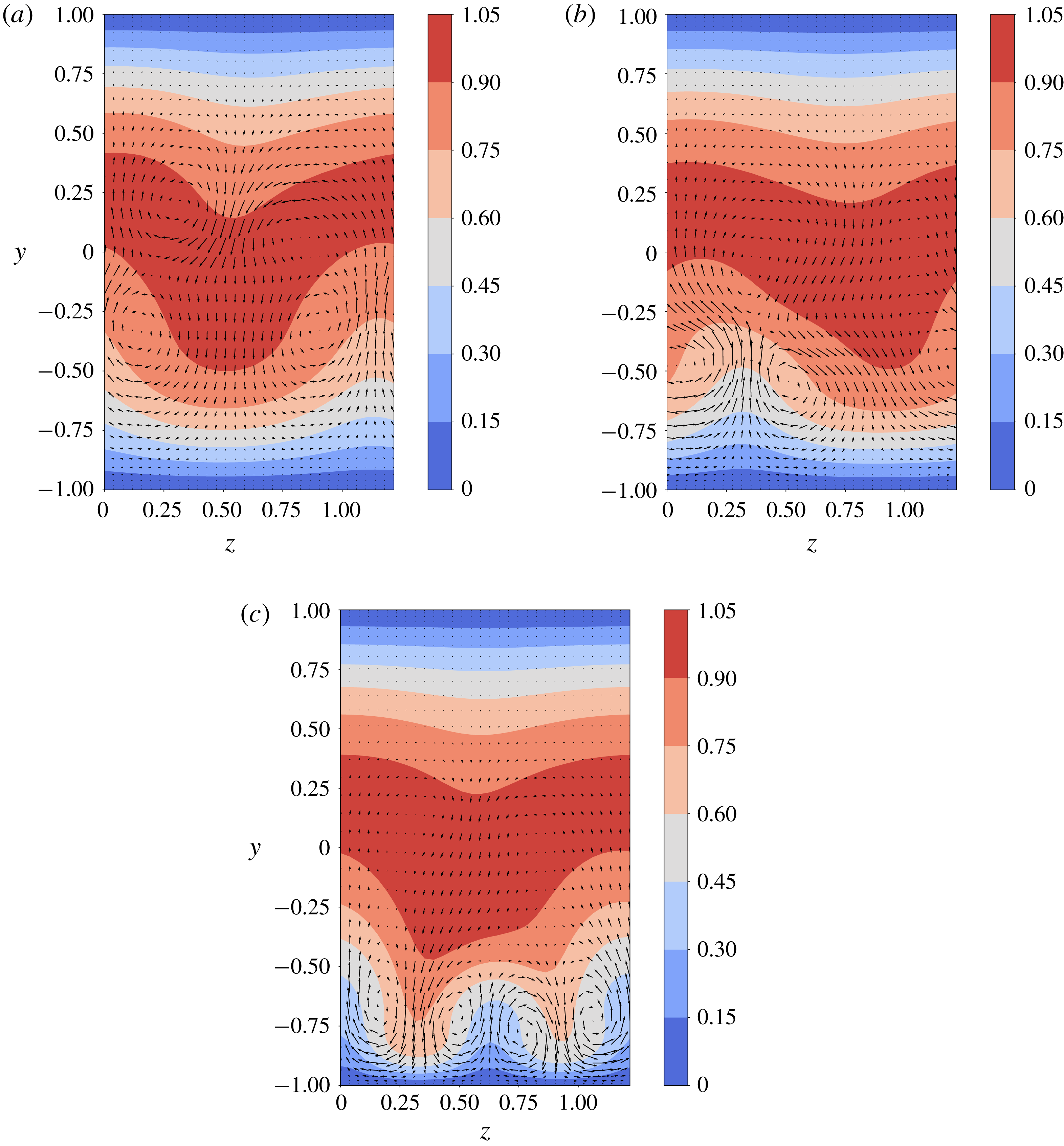
, at which the authors argue that the solution corresponds to the two-streaks mode, here we found that the latter case coincides with the solution that orbits close to the maximum of dissipation (i.e. when the wall shear stress peaks). For instance, a visual representation of the mean flow
 $U$
in the cross-section plane
 $(y,z)$
is provided in figure 5(c) for
 $P_{3}$
. The figure shows that, for this specific point, the streamwise-averaged flow consists of a pair of low-speed streaks generated by quasi-streamwise vortices.
(a) Energy input–dissipation rate for the periodic solution. Values are scaled by their laminar Poiseuille flow solution counterparts (
 $\unicode[STIX]{x1D716}_{lam}$
and
 ${\mathcal{I}}_{lam}$
, respectively). Dashed line corresponds to
 ${\mathcal{I}}/{\mathcal{I}}_{lam}=\unicode[STIX]{x1D716}/\unicode[STIX]{x1D716}_{lam}$
with
 ${\mathcal{I}}_{lam}=\unicode[STIX]{x1D716}_{lam}=8/3Re^{-1}$
. The direction of time is indicated by the arrows. (b) Time evolution of the wall shear stress associated with the streamwise- and spanwise-averaged quantity normalized with the turbulent value,
 $\unicode[STIX]{x1D70F}^{+}$
. The laminar value is indicated with the horizontal line. Time intervals are identical in (a) and (b).

Streamwise-averaged flow
 $\boldsymbol{U}$
. Mean streamwise velocity contours with superposed mean cross-stream vectors for (a)
 $P_{1}$
, (b)
 $P_{2}$
and (c)
 $P_{3}$
(see figure 4).

As shown in figure 5(a,b), although the streak/vortex pattern does not really change for
 $P_{1}$
and
 $P_{2}$
(i.e. both are mainly associated with a single low-speed streak flanked by a pair of streamwise vortices), it appears that the wall-normal position of the eddies slightly changes. In particular, the vortex centres are seen to be displaced away from the lower wall for the
 $P_{1}$
case in comparison to the
 $P_{2}$
case. This has the consequence that the low-speed streak is displaced away from the wall and then the friction exerted along the lower wall is reduced. For comparison, the vortex/streak pattern shown in figure 5(c), where the dissipation rate peaks, is pushed towards the lower wall.
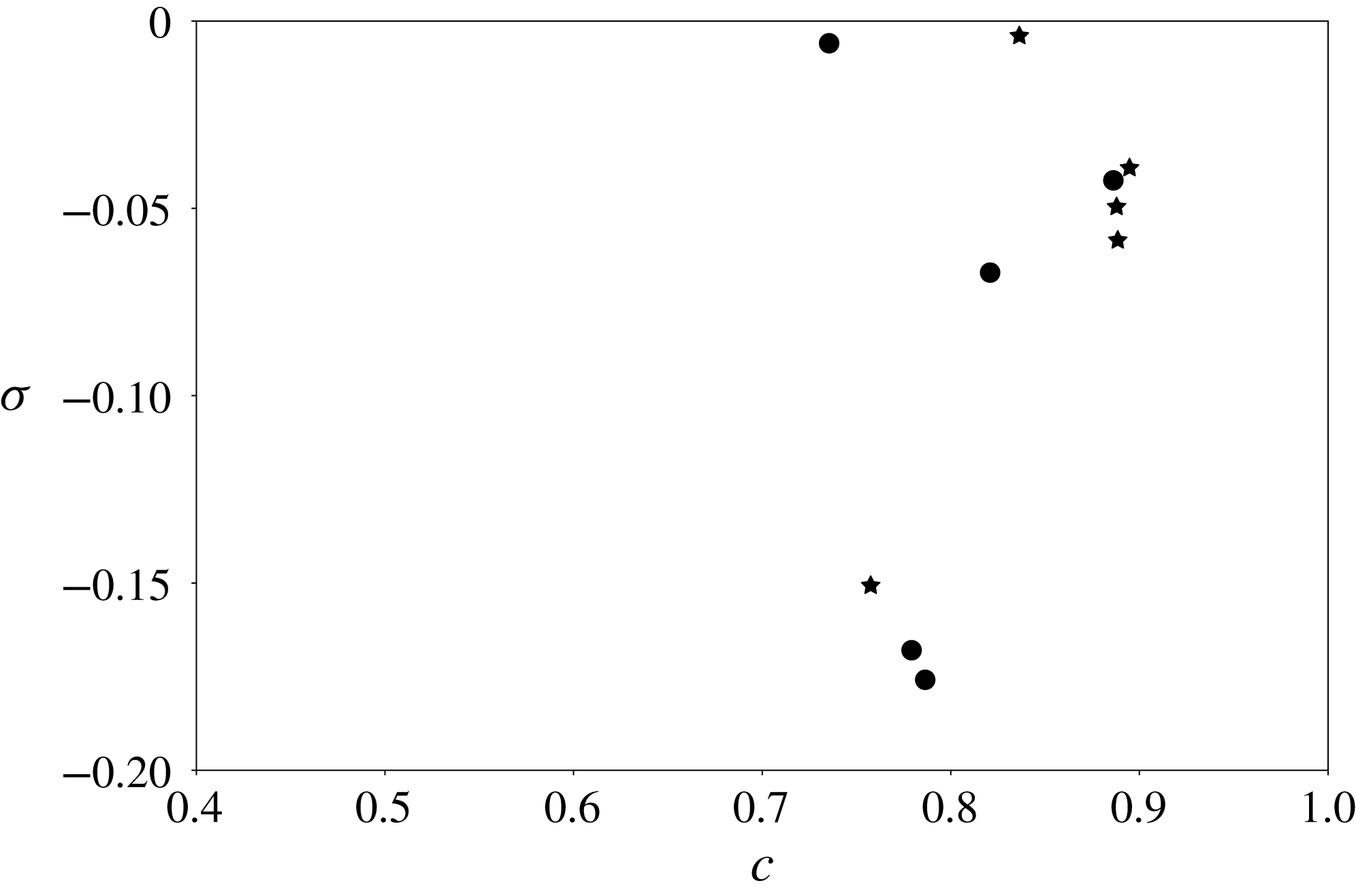
Spectra of the linear stability problem based on the mean flow velocity at
 $P_{1}$
(stars) and
 $P_{2}$
(full circles). The phase velocity is
 $c$
and the temporal growth rate is
 $\unicode[STIX]{x1D70E}$
.

3.4 Two exact coherent states?
In the phase plane,
 $P_{1}$
and
 $P_{2}$
exhibit characteristics of equilibrium states driven by a self-sustained mechanism (Waleffe & Kim Reference Waleffe, Kim and Panton1997). A linear temporal stability analysis is carried out for streamwise-averaged flows
 $\boldsymbol{U}$
that orbit close to
 $P_{1}$
and
 $P_{2}$
, assuming a steady solution (the code is detailed in Alizard (Reference Alizard2015)). In figure 6, we show the spectra for
 $P_{1}$
and
 $P_{2}$
flow cases in the
 $(c,\unicode[STIX]{x1D70E})$
plane, where
 $c$
is the phase velocity and
 $\unicode[STIX]{x1D70E}$
is the temporal amplification rate. The figure shows that the spectra exhibit a quasi-neutral mode for
 $c\approx 0.72$
and
 $c\approx 0.83$
for
 $P_{2}$
and
 $P_{1}$
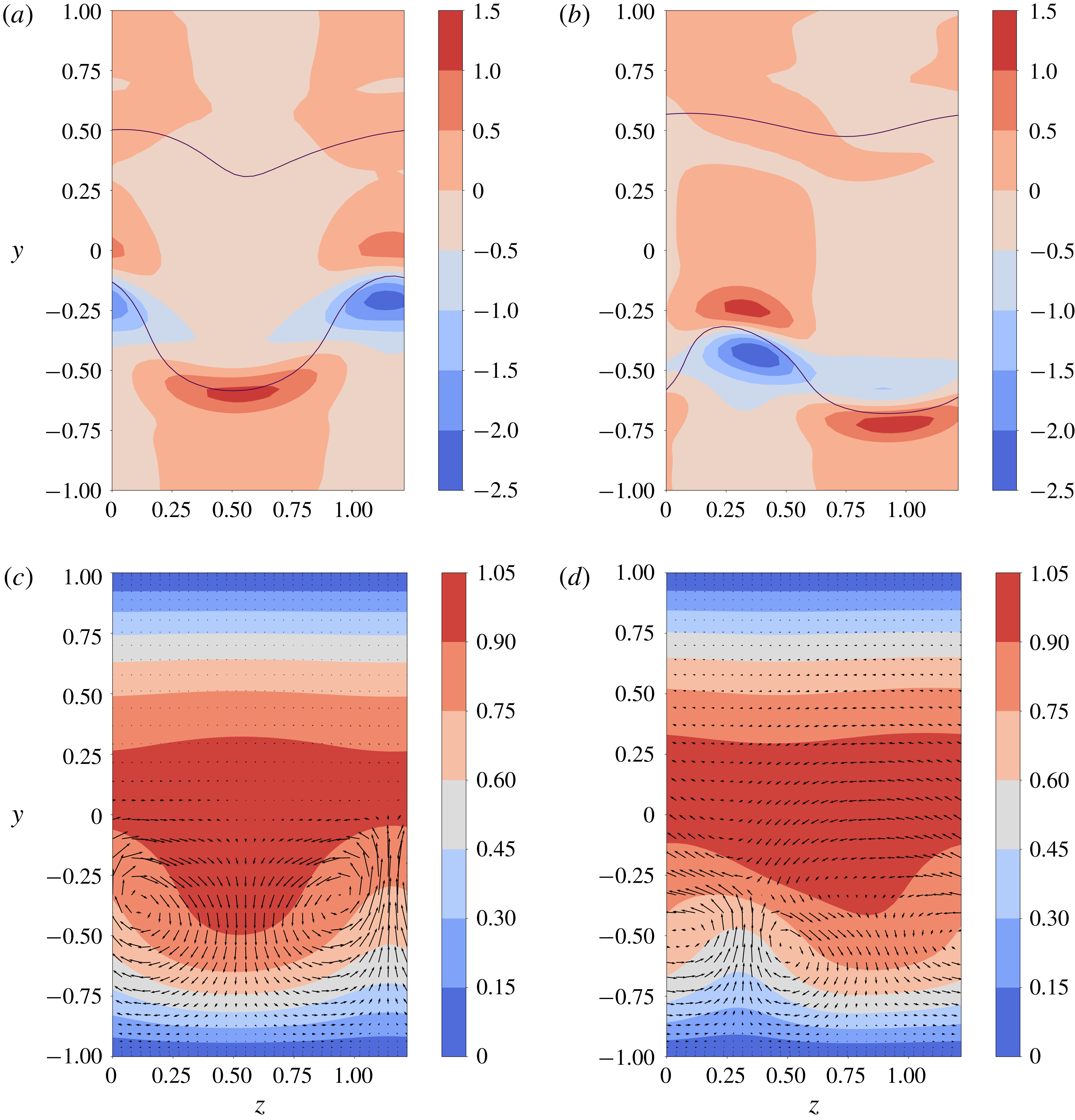
, respectively. We investigate now the regeneration of rolls/streaks by the nonlinear self-interaction of that neutral instability mode and the lift-up effect for both solutions. The spanwise components of the neutral modes are shown in figures 7(a) and 7(b), for
 $P_{1}$
and
 $P_{2}$
, respectively. Both modes exhibit a characteristic sinuous pattern with the energy mainly concentrated near the critical layer, similarly to the lower-branch states found by Wang et al. (Reference Wang, Gibson and Waleffe2007) and Hall & Sherwin (Reference Hall and Sherwin2010) in Couette flow. Rolls are given by
 $$\begin{eqnarray}\left.\begin{array}{@{}c@{}}V_{y}+W_{z}=0,\\ Re^{-1}(V_{yy}+V_{zz})=-P_{y}-\unicode[STIX]{x2202}_{y}(2\hat{v}\hat{v}^{\ast })-\unicode[STIX]{x2202}_{z}({\hat{w}}^{\ast }\hat{v}+{\hat{w}}\hat{v}^{\ast }),\\ Re^{-1}(W_{yy}+W_{zz})=-P_{z}-\unicode[STIX]{x2202}_{y}(\hat{v}^{\ast }{\hat{w}}+\hat{v}{\hat{w}}^{\ast })-\unicode[STIX]{x2202}_{z}(2{\hat{w}}^{\ast }w).\end{array}\right\}\end{eqnarray}$$
For the streak component, we solve iteratively the following equations:
 $$\begin{eqnarray}\left.\begin{array}{@{}c@{}}Re^{-1}(U_{yy}^{c}+U_{zz}^{c})=G^{n}-VU_{y}^{n}-WU_{z}^{n}-\unicode[STIX]{x2202}_{y}(\hat{v}^{\ast }\hat{u} +\hat{v}\hat{u} ^{\ast })-\unicode[STIX]{x2202}_{z}({\hat{w}}^{\ast }\hat{u} +{\hat{w}}\hat{u} ^{\ast }),\\ U^{n+1}=\unicode[STIX]{x1D6FE}U^{c}+(1-\unicode[STIX]{x1D6FE})U^{n},\end{array}\right\}\end{eqnarray}$$
with
 $\unicode[STIX]{x1D6FE}$
a relaxation parameter (
 $0\leqslant \unicode[STIX]{x1D6FE}\leqslant 1$
) and
 $G$
a pressure gradient coefficient that is adjusted to fix the mass flow rate. The amplitude of the Reynolds stress part is provided by the RNL simulation for either
 $P_{1}$
or
 $P_{2}$
events. The numerical implementation of the system (3.5) and (3.6) requires only minor modifications of the RNL solver.
The solutions obtained by solving (3.5) and (3.6) are illustrated in figure 7(c,d). Interestingly, the forcing terms in (3.5) create streamwise vortices that exhibit strong similarities with rolls provided by the unsteady RNL system shown in figure 4(a,b). In addition, under the action of the lift-up effect, the streaky motion derived from the system (3.6) closely resembles the time-dependent solution for both
 $P_{1}$
and
 $P_{2}$
events. Hence, near
 $P_{1}$
and
 $P_{2}$
, the finite-amplitude solution orbits near quasi-equilibrium states where the roll, low-speed streak and streak instability mode have the right pattern and amplitude to almost stay in a mutually self-sustained travelling wave state (Waleffe Reference Waleffe2003). Finally, one may point out that the point
 $P_{1}$
is not identified by Toh & Itano (Reference Toh and Itano2003). However, this discrepancy may well be due to the relatively limited time integration carried out by the previous authors.
Spanwise component of the quasi-neutral mode for
 $P_{1}$
(a) and
 $P_{2}$
(b). The critical layer is reported in full line. Mean streamwise velocity contours with superimposed cross-stream vectors for
 $P_{1}$
(c) and
 $P_{2}$
(d) when assuming a self-sustained equilibrium state.

With the aim to connect turbulent coherent structures near the wall with close passes along the orbit
 $P_{3}$
, statistics obtained by averaging the instantaneous flow (i.e.
 $\boldsymbol{U}+\boldsymbol{u}^{\prime }$
) with respect to the spanwise and the streamwise directions are evaluated at
 $P_{3}$
. For comparison purposes, the state
 $P_{1}$
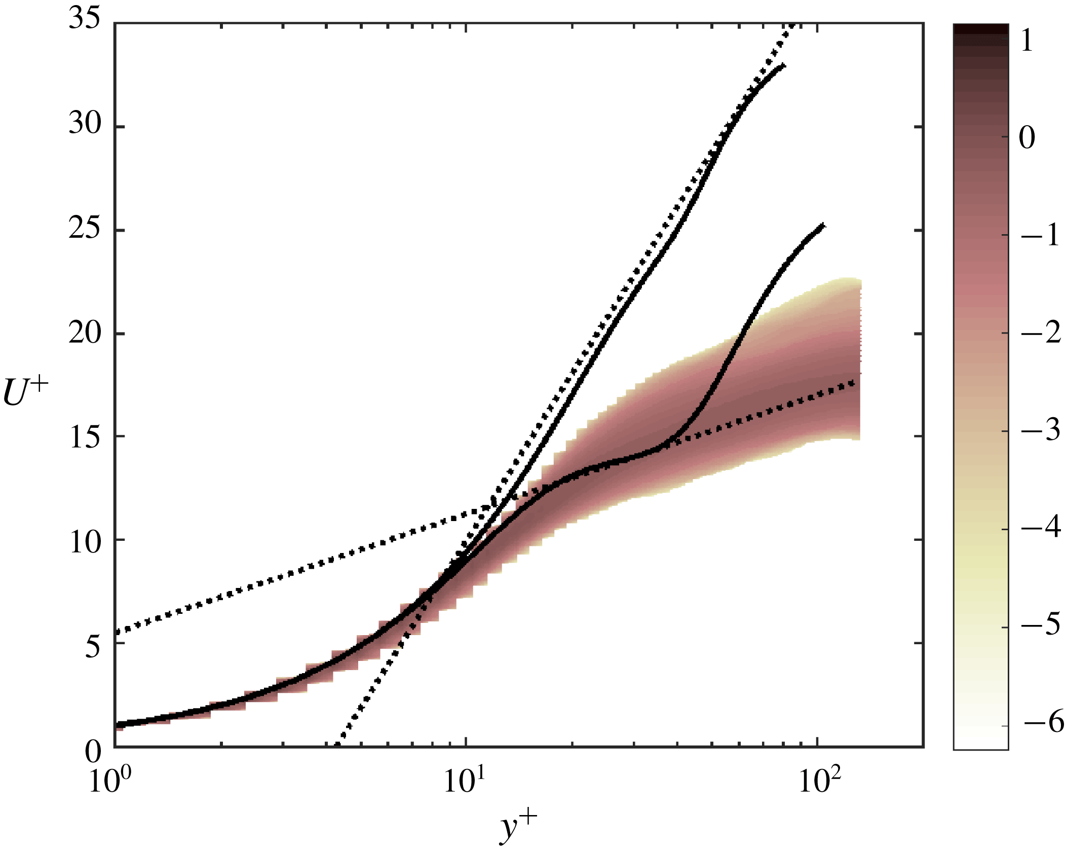
is also considered. In figure 8, we show
 $\overline{U}$
in inner units for
 $P_{1}$
and
 $P_{3}$
events. The standard law of the wall, compounding
 $\overline{U}^{+}=y$
with
 $\overline{U}^{+}=1/\unicode[STIX]{x1D705}\ln y^{+}+C$
, where
 $\unicode[STIX]{x1D705}=0.41$
and
 $C=5.2$
, and the mean velocity associated with an asymptotic state called MDR, the so-called Virk log law,
 $\overline{U}^{+}=11.7\ln y^{+}-17.0$
(Virk et al.
Reference Virk, Mickley and Smith1970; Xi & Graham Reference Xi and Graham2012), are also represented. Figure 8 also shows the p.d.f. obtained from a DNS database, plotted on a logarithmic scale, for locally averaged velocity profiles carried out at each wall-normal position.
Streamwise- and spanwise-averaged flow (full lines):
 $\overline{U}$
as a function of the distance from the lower wall in inner units
 $y^{+}$
for solutions
 $P_{1}$
(low drag) and
 $P_{3}$
(high drag) (see figure 5). The Virk log law and the standard wall turbulence laws are represented in black dashed lines. P.d.f.s from the DNS are presented in log scale. To be consistent with the RNL model, the instantaneous DNS profiles used for the p.d.f.s are averaged over an area of streamwise to spanwise lengths:
 $\unicode[STIX]{x03C0}\times 0.4\unicode[STIX]{x03C0}$
.

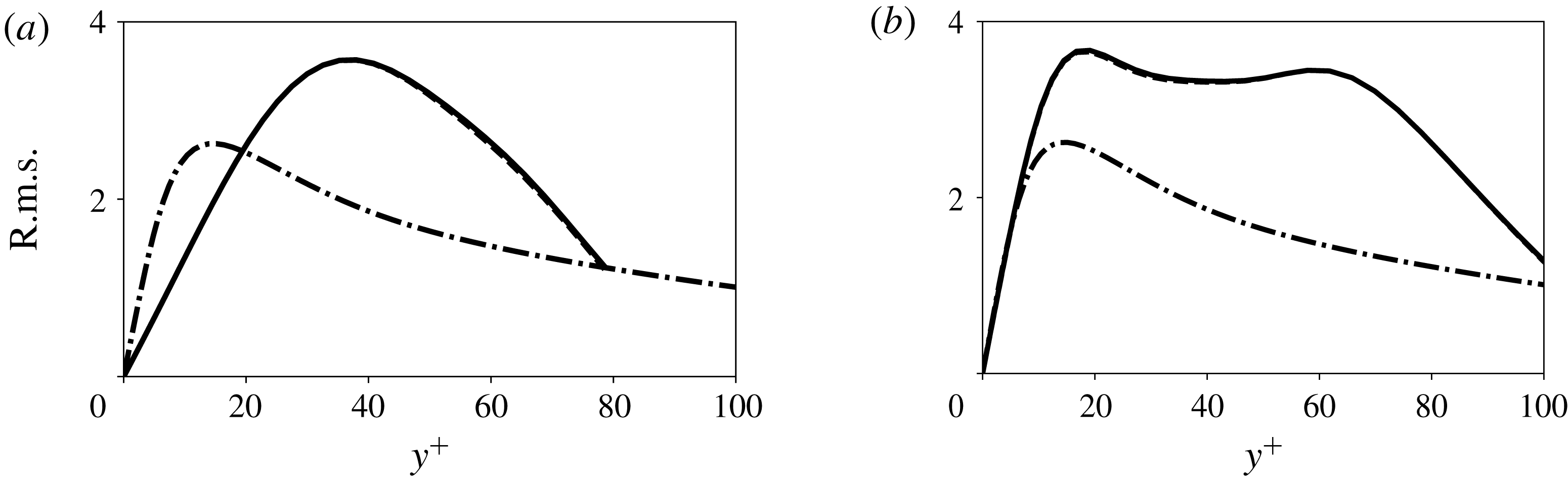
In figure 9, the streamwise r.m.s. velocity profiles as a function of the wall distance are shown in inner units.
Streamwise r.m.s. velocities normalized by
 $u_{\unicode[STIX]{x1D70F}}$
as a function of the distance from the lower wall in inner units
 $y^{+}$
for solutions (a)
 $P_{1}$
and (b)
 $P_{3}$
(see figure 5). The total contribution for the RNL system (i.e.
 $U+u^{\prime }$
) is shown in full line. The contribution of
 $U$
is depicted in dashed lines. Statistics for the turbulent regime obtained by DNS are represented in dotted lines.

Figures 8 and 9 show that the periodic solution displays distinct phases in its dynamics. During the bursting (
 $P_{3}$
event), its trajectory exhibits active turbulence on rare occasions where the friction velocity peaks. In this case, the mean flow profile exhibits a small intermediate region (considering the low value of the friction Reynolds number) where it approaches a logarithmic law with a constant close to the von Kármán value. In addition, at this specific time, the friction Reynolds number
 $Re_{\unicode[STIX]{x1D70F}}\approx 112$
, which is close to the value provided by the full DNS (
 ${\approx}133$
). During
 $P_{1}$
events (i.e. where friction velocity reaches a minimum), the mean flow profile seems to tend to the Virk log-law profile. Nonetheless, although it seems clear from figure 1 that turbulent trajectories experience low-drag events, as shown in figure 8 it appears difficult to compare these states as close excursions through the vicinity of the
 $P_{1}$
(low-drag) solution.
While
 $u_{rms}$
exhibits one peak for
 $P_{1}$
(figure 9
a), a second peak near the wall appears for
 $P_{3}$
events at a wall-normal position
 $y^{+}\approx 15$
(figure 9
b). One may note that the latter peak closely matches the one corresponding to the innermost layer distribution found in DNS. In addition, near the wall, a close match is observed between the minimal RNL system and full DNS. It is also interesting to remark that the contribution of the fluctuating part is negligible for
 $P_{1}$
and
 $P_{3}$
for r.m.s. By recalling that the contribution of the streamwise component due to
 $U$
is associated with the streak, it further indicates the strong correlation between the near-wall peak of the streamwise velocity fluctuations observed in experiments and DNS with streaks. Hence, the periodic edge found by Toh & Itano (Reference Toh and Itano2003) and computed here using a minimal RNL model also exhibits strong similarities with the travelling wave solutions given recently by Park & Graham (Reference Park and Graham2015). The latter authors found ECSs where travelling waves arising from a saddle-node bifurcation induce either a mean velocity profile that resemble the Virk log law (the lower-branch solution) or turbulent mean flow profile (the upper-branch solution). However, a clear connection between this bifurcation and the periodic edge is still missing. Finally, we may remark that the streak spacing during the burst is
 ${\approx}70$
in inner units, which is lower than the near-wall streak spacing observed usually in DNS
 $({\approx}80{-}120)$
. This may explain why the roll/streak inner-layer dynamics observed here appears only during a short time.
4 Discussion
Previously, the Reynolds number, streamwise and spanwise lengths match values given by Toh & Itano (Reference Toh and Itano2003). In the present section, the structural sensitivity of the solution with respect to these three parameters is discussed.
4.1 Effect of the Reynolds number
The increase of the Reynolds number will increase the distance, in phase space, between the turbulent attractor
 $P_{3}$
and the travelling wave solutions
 $P_{1}$
and
 $P_{2}$
. As a consequence, the period of the trajectory on the edge is expected to strongly increase with the Reynolds number. Moreover, the solution
 $P_{3}$
, which captures the key statistics of turbulent shear, is inconsistent with the RNL model for large Reynolds numbers. On the other hand, the two travelling wave solutions (
 $P_{1}$
and
 $P_{2}$
) are lower-branch coherent states. As shown by Wang et al. (Reference Wang, Gibson and Waleffe2007), for large Reynolds number, their asymptotic structure consists of
 $O(1)$
streaks,
 $O(Re^{-1})$
streamwise rolls and a weak streamwise wave that develops on the critical layer, and higher harmonics become negligible. Thus, for these equilibrium states, the RNL model is expected to be consistent with higher values of the Reynolds number.
For large Reynolds numbers, a feasible solution is to extend the RNL equations with the turbulent model. Recently, Rawat, Cossu & Rincon (Reference Rawat, Cossu and Rincon2014, Reference Rawat, Cossu and Rincon2016) and Hwang, Willis & Cossu (Reference Hwang, Willis and Cossu2016) have computed invariant solutions using an overdamped large-eddy simulation (LES) at
 $Re_{\unicode[STIX]{x1D70F}}>10^{3}$
that closely matches with very-large- and large-scale coherent structures observed in turbulent channel flows. In particular, by increasing artificially the Smagorinsky constant to account for the dissipation of surrounding small-scale motions, they were able to isolate a self-sustained exact coherent state in the outer region. Bretheim, Meneveau & Gayme (Reference Bretheim, Meneveau and Gayme2018) extended the RNL model to high Reynolds numbers by using an RNL-LES framework where appropriate streamwise wavenumbers are identified: the ‘band-limited RNL-LES’. The authors showed that such a simulation reproduces successfully some of the most important statistical properties (i.e. the mean velocity and second-order moment profiles). Hence, the use of an RNL system where an additional term modelling dissipative effects of surrounding small scales is included constitutes a promising route to push forward the present analysis to high-Reynolds-number wall-bounded turbulent flows. In this context, invariant states at various scales (i.e. different distances from the wall) could be investigated using this RNL model to identify the dynamical trajectory embedded in the chaotic turbulent attractor.
4.2 Effect of the spanwise length
While edge states (i.e. structures that guide the transition towards a turbulent state) have been widely studied in minimal periodic domains (i.e. MFU), the resulting constrained dynamics may prevent a direct connection with experimental observations of an incipient turbulent spot generated by localized initial perturbation. In this context, some authors (Schneider, Marinc & Eckhardt Reference Schneider, Marinc and Eckhardt2010; Khapko et al. Reference Khapko, Kreilos, Schlatter, Duguet, Eckardt and Henningson2013; Eckhardt Reference Eckhardt2014) have recently computed spanwise and/or spanwise–streamwise localized edge states in sufficiently extended computational domains for Couette and asymptotic suction boundary layer (ASBL) flows.
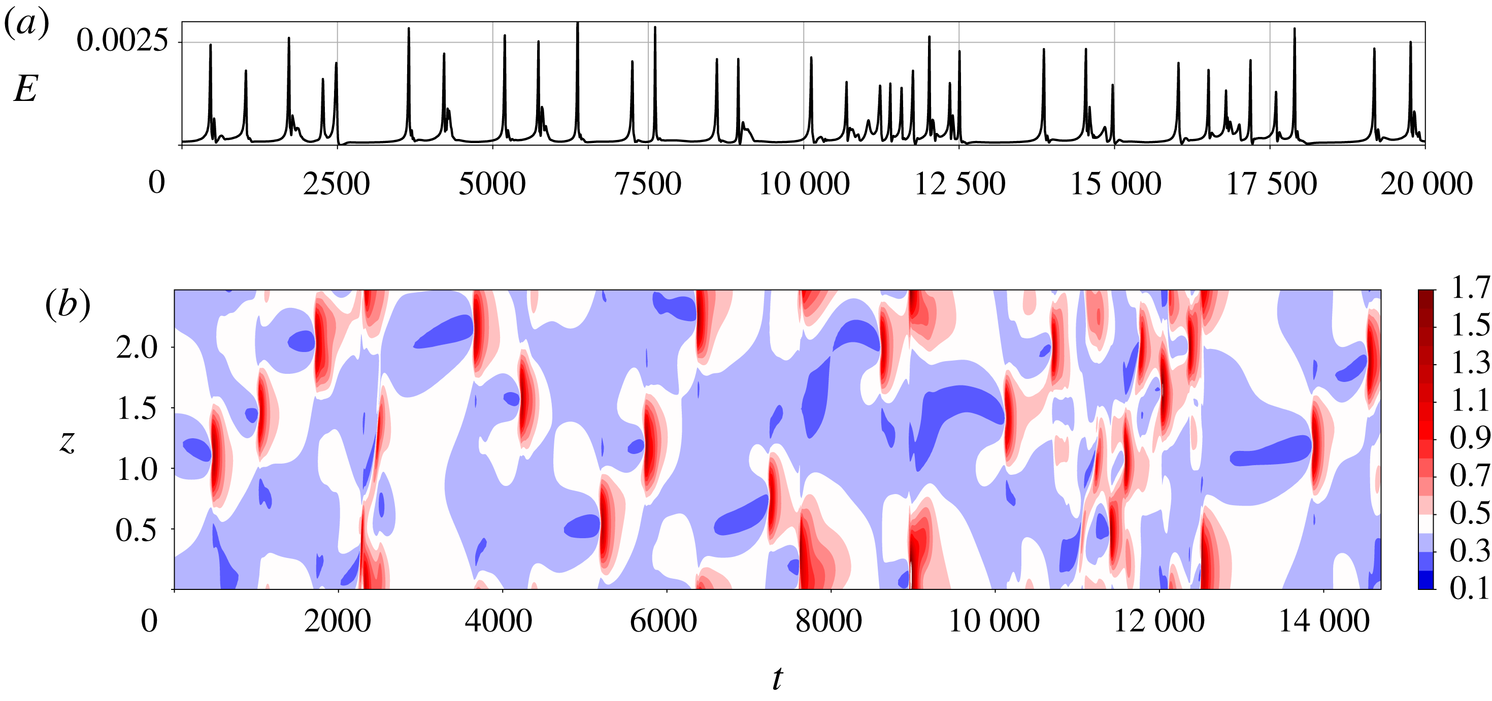
RNL simulation. Edge solution for
 $Re=3000$
,
 $L_{z}=0.8\unicode[STIX]{x03C0}$
and
 $L_{x}=\unicode[STIX]{x03C0}$
: (a) time evolution of kinetic energy of the fluctuation; and (b) spanwise and time evolution of the wall shear stress, normalized with the turbulent value.

In this section, we investigate the evolution of the periodic solution obtained at the MFU when doubling both the spanwise extent and number of spanwise Fourier modes. For that purpose, we construct a spanwise localized solution by windowing the periodic solution obtained at the MFU (Gibson & Brand Reference Gibson and Brand2014). In figure 10(a,b), we report RNL results given by the edge-tracking algorithm for
 $L_{z}=0.8\unicode[STIX]{x03C0}$
. Figure 10(b) shows that the solution is mostly localized in the spanwise direction, in contrast with the previous case (
 $L_{z}=0.4\unicode[STIX]{x03C0}$
) for which the domain is almost entirely filled. Similar behaviour was recently observed by Xi & Bai (Reference Xi and Bai2016) using DNS. In particular, we observe the alternation of calm phases and bursting events before being shifted in the spanwise direction. However, the solution is not periodic any more, and low-speed streaks are shifted towards either the right or the left direction, similarly to what is observed for the ASBL case (Khapko et al.
Reference Khapko, Kreilos, Schlatter, Duguet, Eckardt and Henningson2013). In addition, the skin friction reaches a higher peak than its minimal box counterpart (see figure 3). Nevertheless, we cannot draw definite conclusions on a chaotic behaviour or if a periodic state exists because the transient regime appears to be extremely long for such a case.
4.3 Effect of the streamwise length
The streamwise length
 $L_{x}=\unicode[STIX]{x03C0}$
, or
 $L_{x}^{+}=410$
, is close to a minimal streamwise unit. Under this restriction, large-scale motions are exactly two-dimensional, infinitely long structures, prevented from evolving spatially in the flow direction, but can evolve in the cross-stream plane; hence, the dynamics is thus basically temporal rather than spatio-temporal. DNS of channel flow with a minimal streamwise flow unit were performed by Toh & Itano (Reference Toh and Itano2005) for relatively low Reynolds numbers (
 $Re_{\unicode[STIX]{x1D70F}}=$
137 and 349), and extended by Abe, Antonia & Toh (Reference Abe, Antonia and Toh2018) up to
 $Re_{\unicode[STIX]{x1D70F}}=1020$
. Large-scale structures observed in large computational domains are shown to exist, even in a minimal streamwise flow unit. Moreover, the authors observed a co-supporting cycle where large-scale structures are generated by the collective behaviour of near-wall structures, and the generation of the latter is in turn enhanced by the large-scale structures.
The extension of the present results, based on an RNL model, to very large streamwise domains is not just a numerical challenge; it mainly raises the issue of the decomposition between a (streamwise-averaged) base flow and fluctuations (travelling wave).
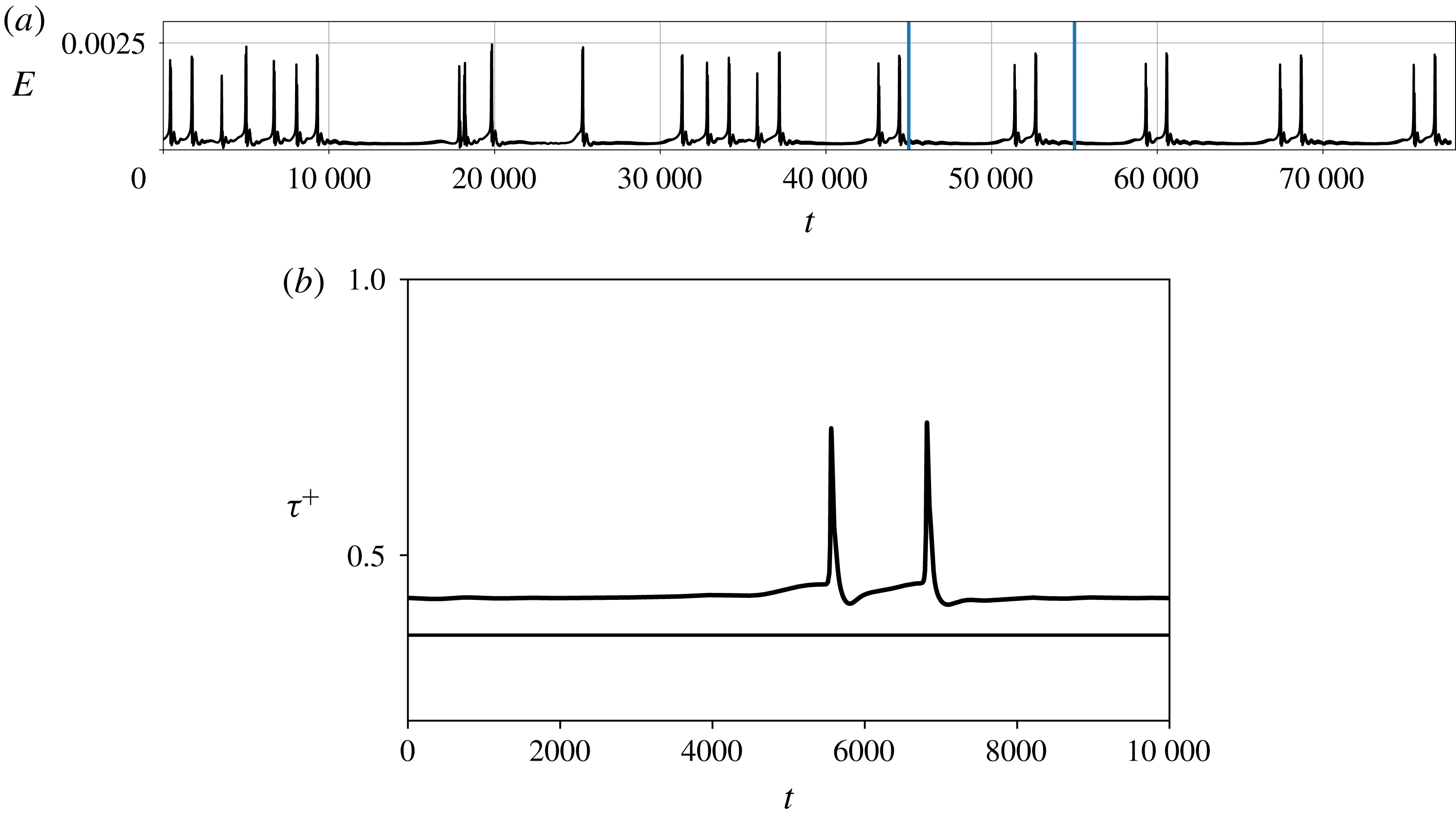
Nonetheless, the effect of small variation of streamwise length has been investigated. In figure 11, we report a minimal RNL simulation for the same Reynolds number and spanwise extent but with a slightly smaller length in the streamwise direction:
 $L_{x}=0.9\unicode[STIX]{x03C0}$
. After a long transient regime, the solution reaches a periodic state where a pair of bursting events are separated by very long quiescent intervals
 $({\approx}6000)$
. Figure 11 shows that the solution exhibits similar behaviour to that observed previously, for
 $L_{x}=\unicode[STIX]{x03C0}$
. In particular, for bursting events, the flow pattern also exhibits a competition between the fundamental and its first harmonic spanwise Fourier mode, i.e.
 $E_{1}$
and
 $E_{2}$
(not shown here for the sake of conciseness). However, such an event appears to happen within a periodic process that has strongly extended in time. The latter remark is also consistent with the minimal box for self-sustained turbulence, which was close to the one used by Toh & Itano (Reference Toh and Itano2003).
RNL simulation. Edge solution for
 $Re=3000$
,
 $L_{z}=0.4\unicode[STIX]{x03C0}$
and
 $L_{x}=0.9\unicode[STIX]{x03C0}$
: (a) time evolution of kinetic energy of the fluctuation; and (b) time evolution of the streamwise wall shear stress normalized with the turbulent value for a time interval represented by the vertical lines in panel (a). The laminar value is indicated with the horizontal line.

5 Conclusion
In this paper, we show that the nonlinear periodic solution computed by Toh & Itano (Reference Toh and Itano2003) and Zammert & Eckhardt (Reference Zammert and Eckhardt2014) and more recently by Rinaldi et al. (Reference Rinaldi, Schlatter and Bagheri2018) using DNS can be tracked with a restricted nonlinear (RNL) system where only a single streamwise Fourier mode is retained for the fluctuation. In particular, similar characteristics are found for both simulations such as long quiet states, shifted states along the spanwise direction and bursting events where flow patterns exhibit either a single streak or two streaks that compete with each other. Interestingly, the mean flow and r.m.s. profiles provided by the RNL system exhibit strong similarities with wall-bounded turbulent statistics obtained both in experiments and in DNS for data extracted when the mean friction velocity (i.e. averaged in streamwise and spanwise directions) peaks. The friction Reynolds number computed by collecting data at the burst almost matches the one derived from a DNS database. The present results are then consistent with those of Bretheim et al. (Reference Bretheim, Meneveau and Gayme2015) and Farrell et al. (Reference Farrell, Ioannou, Jiménez, Constantinou, Lozano-Durán and Nikolaidis2016), who have found that a realistic turbulence state can be maintained with an RNL system with low streamwise Fourier components for the fluctuation. Furthermore, the contributions of the streamwise-averaged quantities and streamwise-varying fluctuations about that mean onto the r.m.s. extracted at the maximum drag indicate that its peak is mainly due to the mean flow variables. This further supports that near-wall streaks are ‘active’ scales in the sense that they are mainly responsible for the turbulent energy production and momentum transfer in comparison with the fluctuating part. Interestingly, the present analysis also shows that the trajectory of the periodic solution initially found by Toh & Itano (Reference Toh and Itano2003) exhibits close excursions near an asymptotic state with MDR. Hence, the solution seems to be closely tied to intermittent behaviour found in near-wall turbulence for low-Reynolds-number flows where chaotic movement of turbulence is seen to spend some time around high- and low-drag events. In particular, our study shows that the periodic solution seems to be intimately connected to the lower- and upper-branch states found by Park & Graham (Reference Park and Graham2015) in plane channel flows. However, the link between this periodic solution and the upper- and/or lower-branch solutions of Park & Graham (Reference Park and Graham2015) remains unclear. It needs to be pointed out that, in comparison to the work of Park & Graham (Reference Park and Graham2015), no symmetry conditions are imposed here, in neither time nor space, which allows the solution to travel around different fixed points. Nevertheless, the results obtained using the RNL system agree with the edge-tracked solution recently found by Xi & Bai (Reference Xi and Bai2016) using the full Navier–Stokes equations for a similar flow case (i.e. trajectories closely approaching an MDR state are also found).
In addition, while it seems clear from statistics provided by the DNS database that some turbulent trajectories pass through low-drag events, the present results seem also to indicate a connection in the phase space between the turbulent attractor, associated high-drag events, and travelling wave equilibrium states, associated with low drag. A projection of the dynamical trajectory onto a more appropriate two-dimensional plane seems to be necessary to draw a definite conclusion.
Our analysis also gives a strong indication that more complex nonlinear finite-amplitude solutions than travelling wave solution may be well approximated by a minimal RNL system. In that respect, it extends the recent study carried out by Pausch et al. (Reference Pausch, Yang, Hwang and Eckhardt2018), focusing on travelling wave states associated with upper-branch solutions in both Couette and plane channel flow. From this discussion, it appears that investigations of invariant solutions using the RNL system can provide an efficient tool to select appropriate streamwise wavenumbers for RNL simulation aiming to reproduce turbulence in wall-bounded flows. It also further confirms the important role of the mean flow in shaping invariant states for wall-bounded flows. This is consistent with other models relying on mean flow analysis, such as the resolvent operator technique (Sharma & McKeon Reference Sharma and McKeon2013). In particular, Sharma et al. (Reference Sharma, Moarref, McKeon, Park, Graham and Willis2016) have recently shown that exact invariant solutions lying on the edge for channel geometries are well approximated using a projection onto a limited number of resolvent modes.
In the present study, it is observed that a long transient time is necessary to reach an invariant state. Hence, the use of an RNL system may be useful to provide an initial condition for tracking a periodic edge having long quiescent phases with DNS.
Finally, to better characterize similarities between observations at the MFU and states lying on extended domains, a spanwise localized state has been investigated by doubling the width of the computational box and windowing the periodic solution obtained at the MFU. We show that the solution bears a strong resemblance to the one obtained in a minimal box (i.e. alternation of calm phases and bursting events, spanwise shifted pattern) with the exception of periodicity. In this case, the edge dynamics is erratic. In a future work, the spanwise extent should be further increased to prevent any influence of periodicity. The RNL system may thus provide an efficient model to characterize complex spanwise localized states that may constitute nuclei for the transition of turbulence.
Acknowledgements
This work was granted access to the HPC resources of the FLMSN, ‘Fédération Lyonnaise de Modélisation et Sciences Numériques’, partner of EQUIPEX EQUIP@MESO.