


1. Introduction
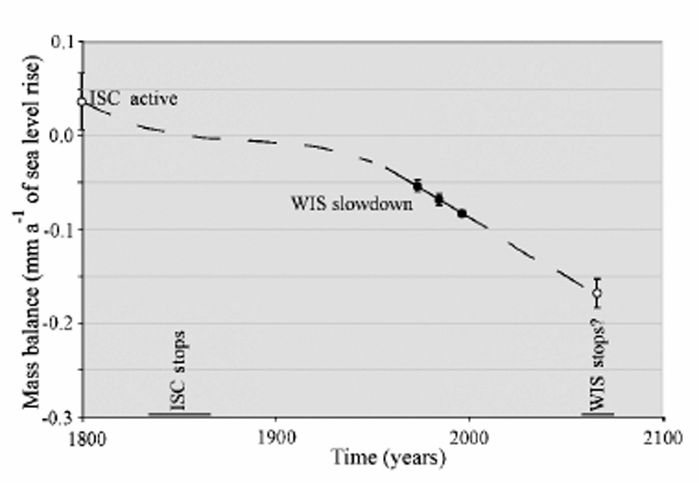
The modern volume of the West Antarctic ice sheet (WAIS) is equivalent to a sea-level rise of up to 6 m. This represents only a fraction of the Late-glacial volume of the ice sheet, most of which was lost during the last ∼10 000 years when the WAIS experienced grounding-line retreat at rates averaging ∼100 m a–1 (Reference Conway, Hall, Denton, Gades and WaddingtonConway and others, 1999). The behavior of the WAIS in recent centuries and decades has been highly unstable and is at present inconsistent in some regions with the postglacial trend of retreat and shrinkage (Reference Fahnestock, Abdalati, Joughin, Brozena and GogineniFahnestock and others, 2001; Reference Joughin, Tulaczyk, Bindschadler and PriceJoughin and Tulaczyk,2002). The instability in WAIS behaviorcanbe attributed to changes in flow of fast-moving ice streams and outlet glaciers that carry almost all of the ice discharging from the ice sheet. At the present time, while Pine Island Glacier experiences rapid thinning (Reference RignotRignot, 2001; Reference Shepherd, Wingham, Mansley and CorrShepherd and others, 2001), the drainage basins of the Ross ice streams have, on average, a strongly positive imbalance (Joughin and Tulaczyk, 2002). The main reason for the thickening in this region is the shut-down of Ice Stream C (ISC) ∼150 years ago combined with a marked slow-down of Whillans Ice Stream (WIS) averaging about 5 m a–2 between 1974 and 1997 (Fig. 1). If this deceleration continues at its current rate, the outflow of ice from WIS will cease in ~ 70 years. This event would increase the contribution of this section of the WAIS to global sea-level change to nearly –0.2mm a–1 (negative sign denotes sea-level fall) (Fig. 2). The stoppage of WIS would also constitute a large perturbation to the mass balance of the Ross Ice Shelf, which would receive from the Ross ice streams only ~ 40 km3 of ice per year, down from ∼70 km3 a–1 at present and ∼100km3 a–1 before the stoppage of ISC. This perturbation, particularly if combined with a possible near-future increase in bottom melting rates (Rignot and Jacobs, 2002), could help destabilize the ice shelf, causing its retreat or even a complete break-up.
Location map showing ice-velocity distribution (color scale) overlain on top of a satellite image of ice-sheet (Reference JoughinJoughin and others, 1999). The area is focused on WIS (formerly Ice Stream B) and ISC.

Evolution of ice fluxes out of the Ross Sea sector of the WAIS over three centuries, based on data from Reference Joughin, Tulaczyk, Bindschadler and PriceJoughin and Tulaczyk (2002) and Reference Joughin, Tulaczyk and EngelhardtJoughin and others (2003). Ice fluxes are expressed in mm a–1of sea-level change. The three filled circles show the effects of the slow-down of the lower part of WIS as captured by data collected in 1974, –1985 and 1997. Error bars reflect only the 2σ uncertainty in velocity measurements.The two open circles show our estimates of ice fluxes out of the region before the stoppage of ISC and after the possible near-future stoppage of WIS. In this case, error bars are based on estimates only.
Previous analytical modeling indicates that the slowdown of WIS is most likely due to either freeze-on-driven strengthening of the ice-stream bed or a decrease in driving stress (Reference Joughin, Tulaczyk, Bindschadler and PriceJoughin and others, 2002). In the latter case, the slow-down could be unsustainable, because with time a decrease in ice discharge should act against the initial tendency of the driving stress to decrease. Bed strengthening, on the other hand, can be a runaway process, which is capable of bringing an ice stream to a complete stoppage (Reference S.M., Kamb and EngelhardtTulaczyk and others, 2000b). One of the serious limitations of our previous analytical modeling was its inability to examine the possible influence of basal water import from upstream on bed strengthening (Reference Joughin, Tulaczyk, Bindschadler and PriceJoughin and others, 2002). Yet calculations of melting and freezing rates beneath WIS do suggest that while the lower part of the ice stream may be experiencing basal freeze-on (and bed strengthening), its upstream regions are likely to experience basal melting (Reference Joughin, Tulaczyk and EngelhardtJoughin and others, 2003). Similar conclusions have been drawn by Parizek and others (2002) for Ice Stream D, based on their model calculations of basal melting and freezing. If the basal meltwater can be imported into the regions experiencing freezing at sufficiently high rates, excessive bed strengthening and complete ice-stream stoppage could be averted.
We have recently constructed a new model of an ice stream with an evolving till bed, which can be used to investigate the observed slow-down of WIS. The model includes a simple parameterization of basal water transport to investigate how much water, if any, would have to be supplied to the bed of WIS to prevent its complete stoppage. Previously, we have used the same numerical code to simulate the stoppage of ISC. This experience indicated that relatively small changes in the width of this ice stream could switch it between steady (no shut-down) and unsteady (shut-down) modes. Hence, we have also tested the sensitivity of the WIS model to variations in width.
2. Model Description
2.1. Equations
In simulations of the slow-down of WIS, we have used a numerical ice-stream model that was developed to investigate whether the shut-down of ISC may have been caused by freeze-on-driven strengthening of till (Reference S.M., Kamb and EngelhardtTulaczyk and others, 2000b; Reference Bougamont, Tulaczyk and JoughinBougamont and others, 2003). This numerical model explicitly couples a module describing ice thermodynamics with an evolving till bed. This model is easily adapted to WIS, since only the prescribed geometry (bed topography, ice-stream width) has to be adjusted. The model domain includes the main trunk of the ice stream (275km long), and two ice-stream tributaries (160 km long).
The center-line velocity equation is modified from Reference RaymondRaymond (1996; see also Reference S.M., Kamb and EngelhardtTulaczyk and others, 2000b), and assumes that the driving stress is balanced by a combination of basal resistance and marginal stress. All other forces are ignored.

where W is the width of the ice stream (m), H is the ice thickness (m) and τd is the driving stress (Pa) (τd =
PigHα, where A is the ice density (kg m–3), τb is the basal stress (Pa), g is the constant of acceleration due to gravity (ms–2) and α is the surface slope). The surface velocity Us, includes a basal sliding component and an internal deformation component  In the latter, B is the stiffness parameter (Paa1/3), and we use the Arrhenius relationship (with activation energies as given in Reference Jackson and KambJackson and Kamb (1997)) to compute a column-averaged value of B from vertical ice-temperature profiles calculated in the model. Integration of equation 39 from Reference RaymondRaymond (1996) gives the average ice velocity in the along-flow direction, u =
0.8Us
(assuming n = 3).
Knowing the geometry and the velocity field for the ice stream, we can impose ice conservation using a flow-band equation (Reference PatersonPaterson,1994, p. 256–257):
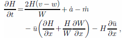
where t denotes the time (years), the first righthand-side term is the influx of ice across lateral ice-stream boundaries (expressed per unit area, just like the accumulation rate; m a–1), v is the transverse ice velocity (m a–1) across the ice-stream margin (positive inward and negative outward), w is the velocity of margin migration (sign convention as for v), ȧ is the accumulation rate (parameterized by varying it with elevation from 0.08ma–1 at the grounding zone to 0.15 ma–1 at the onset to reflect existing data (Reference Giovinetto, Waters and BentleyGiovinetto and others, 1990; Reference Vaughan, Bamber, Giovinetto, Russell and CooperVaughan and others, 1999)), and ṁ is the basal melting/freezing rate (m a–1). Ice flow from Ice Stream A (ISA) into WIS is accommodated by adding a constant ice flux across the lateral boundary of the lower part of the trunk (at ~ 8 km3 a–1; Reference Joughin, Tulaczyk, Bindschadler and PriceJoughin and Tulaczyk, 2002).
The basal stress τb in our model is dependent on the till void ratio, e, and the relation between the two quantities is based on laboratory experiments (Reference Tulaczyk, Kamb and EngelhardtTulaczyk and others, 2000a, equation 3d; Reference Kamb, Alley and BindschadlerKamb, 2001):

where a and b are empirical constants. According According to this equation, basal resistance increases exponentially as the void ratio decreases.
To calculate basal melting/freezing rates, the basal temperature gradient must be determined. We compute the temperature field in the ice stream, using a two-dimensional equation including vertical diffusion as well as vertical and horizontal advection (Reference Hooke and LeHooke, 1998, p. 79–80):

where κ is the thermal diffusivity in the ice (m2 a–1), T is the ice temperature (°C), and ws and wb are respectively the vertical velocity at the surface and the base of the ice column (ma–1). As is customary, the horizontal diffusion term has been omitted (Reference Hooke and LeHooke, 1998, p. 79). The linear parameterization of vertical ice velocity used in Equation (4) is a fair assumption for West Antarctic ice streams, whose internal ice deformation contributes little to their forward motion (Reference Kamb, Alley and BindschadlerKamb, 2001).
For thermal boundary conditions, we took basal temperature equal to the pressure-melting-point temperature everywhere (Reference HughesHughes, 1998, p. 294–295) and prescribed temporally constant surface temperatures. We used a small atmospheric lapse rate of 0.004 "Cm–1 to calculate the surface temperature distribution by assuming linear dependence on surface elevation. This lapse rate is lower than the typical range of atmospheric lapse rates (0.006–0010 ˚Cm–1). It has long been recognized that there is a regional anomaly in the vertical distribution of temperature in the study area (Reference Giovinetto, Waters and BentleyGiovinetto and others, 1990). The value used here was calculated by fitting 10 m temperatures at Byrd Station, as well as from several locations on WIS, Siple Dome and ISC (Reference Kamb, Alley and BindschadlerKamb, 2001; personal communication from H. Engelhardt, 2001).
The melting/freezing rate ṁ affects the bed strength and ice velocity by adding water to, or subtracting it from, the till layer, thereby increasing or reducing the till void ratio (Equation (3)). The rate is computed from the energy-balance equation (Reference Anandakrishnan and AlleyTulaczyk and others, 2000b):

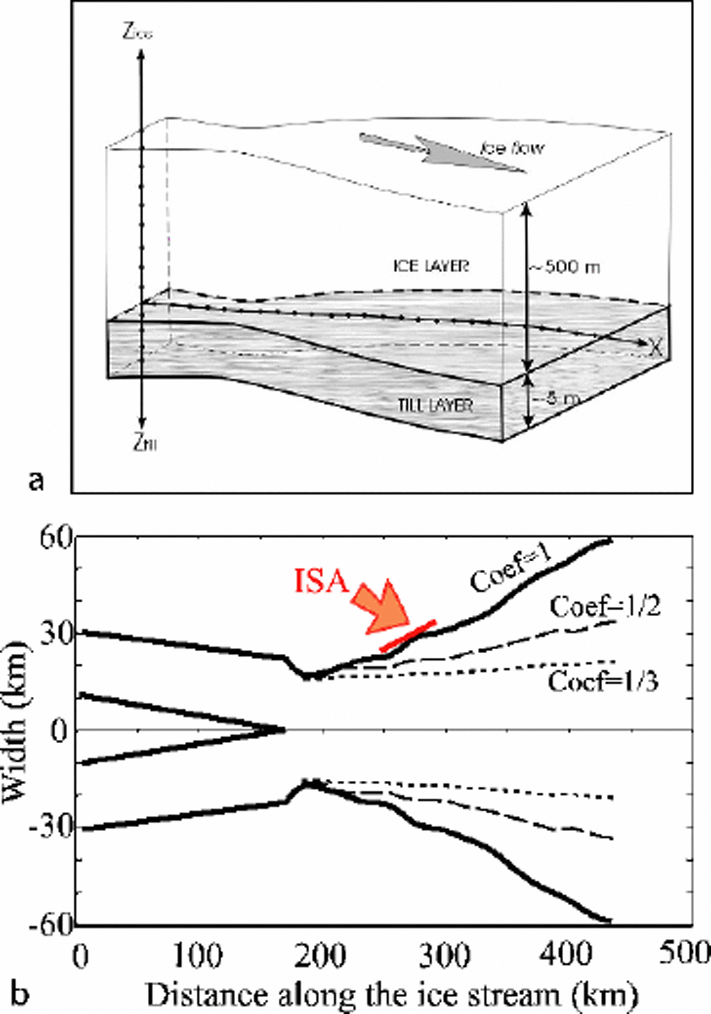
where G is the geothermal flux (Wm–2) , Ki is the thermal conductivity of ice (J m–1s–1 K–1), θ b is the basal temperature gradient (°C m–1) (negative quantity in our coordinate system; Fig. 3a), L is the latent heat (J kg–1) and P i is the ice density (kg m–3).
(a) Sketch illustrating the arrangement of horizontal (ice) nodes and vertical (temperature) nodes in our flowline model. (b) Distribution of width along ice-stream axis. The bold line labeled Coef= 1 represents the modern distribution, and the two dashed lines show the narrower width distribution assumed in some of our numerical experiments. The red arrow labeled ISA shows the place in the model where we input the ice discharging from ISA.
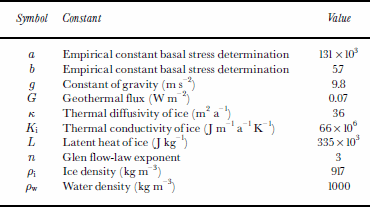
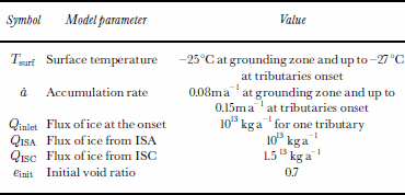
Values of constants and constant parameters used in the model are summarized in Tables 1 and 2.
Values of constants used in the model
Values of constant parameters used in the model
2.2. Numerical methods
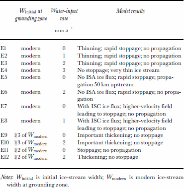
At the beginning of each experiment, the model is initialized by prescribing boundary conditions emulating the modern state of WIS, and the model is run in a “spin-up” mode. In this mode, no changes in boundary conditions are imposed and no feedback between the ice module and the till–bed module is allowed. Consequently the model converges toward a steady state. Our arbitrary condition for deciding when this steady state is achieved states that the year-to-year variation in the velocity field must become small everywhere (typically < 1 m a –1) . Once the velocity field converges to this criterion, we turn on the feedback between the ice and the till modules by allowing the till strength to respond to the calculated basal melting/freezing rates (Equations (3) and (5)). The horizontal spatial resolution is 5 km for an ice-stream length of 435km (160 km of tributaries, 275 km of main trunk). We solve the mass-balance and thermal equations (Equations (2) and (4)) using a finite-difference method with a semi-implicit scheme (both central and upward (for horizontal advection in Equation (4)) scheme), which allow us to run the model with a larger time-step than with the explicit method previously used (up to 20 times faster). We have not observed significant differences in output of the initial runs performed with the explicit integration scheme and similar later runs done using the semi-implicit scheme. Out of the several dozens of numerical experiments that we have performed as part of this work, we discuss here 12 representative experiments (summarized in Table 3) and referred to in the text as E1–E12. These experiments have been selected because they are relevant to our goal of assessing whether the current slow-down of WIS will result in a near-future stoppage.
Description of the 12 experiments discussed here
3. Experimental Design
3.1. Influence of basal drainage
In several experiments, we introduced a water system that allowed flow of water to take place between the ice and the till layer (E1–E4). The presence/absence of water drainage is still controversial as far as its control over ice-stream behavior is concerned (Reference Alley, Anandakrishnan, Bentley and LordAlley and others, 1994; Reference Anandakrishnan and AlleyAnandakrishnan and Alley, 1997; Reference Anandakrishnan and AlleyTulaczyk and others, 2000b; Parizek and others, 2002). We propose here a simple way to examine the potential role which the basal water system may play in the near-future evolution of the observed slow-down of WIS.
Notes: Winitial is initial ice-stream width; Wmodern is modern ice-stream width at grounding zone.
The assumed basal water system is present everywhere beneath the ice base. We drive it by prescribing a constant realistic amount of water that enters the system at its upstream end (onset of the tributaries). The maximum amount of water that we force into the system is 1305 m3 a–1 per meter width of the onset, equivalent to the addition of ∼3mm a–1 of water to each meter squared of the ice-stream bed. Previous estimates of basal melting rates within the drainage basin of WIS and neighboring ice streams indicate that water-influx rates into the part of WIS simulated here may be of the order of 10–1000m3 a–1 per meter width (equivalent to a melting rate of ∼0.01 to ∼1mm a–1 per unit area of ice-stream bed) (Reference Alley, Blankenship, Bentley and RooneyAlley and others, 1986; Reference Tulaczyk, Hunke, Joughin, Bougamont and VogelTulaczyk and others, 2001; Parizek and others, 2002). Once the set water volume is added at the tributary onsets, it is tracked through each node. At each time-step, if at a given node the basal melting/freezing rate is positive (melting), water in the basal system is assumed to simply pass the node without gaining or losing any volume. If the basal melting/freezing rate is negative (freezing), then water from the basal system is used first to satisfy the freezing rate. Only once all of the basal water is depleted upstream of (and at) a given node, will the basal freezing be satisfied through withdrawal of pore water from till.
The basal water is never used in the model to decrease the basal resistance to ice-stream motion. Rather, we assume that basal resistance is still set by local exchange of water between the ice base and the till. We just make it harder for freeze-on-driven bed strengthening to occur by providing a large reservoir of latent heat in the form of the basal water system. If we were to assume that all or some of the added basal water acts to decrease the basal shear stress, the calculated shear heating would be lower. This would either decrease basal melting rates or even switch the basal energy balance to freezing, necessitating that some of the water from the basal system be used to satisfy the freeze-on. Hence, our treatment of the basal water system as a simple reservoir of latent heat represents a conservative assumption, from the point of view of checking how much basal water is needed to prevent ice-stream stoppage.
3.2. Ice influx from ISA and ISC
ISA supplies to the lower part of WIS avolume of ice equivalent to almost one third of the total surface accumulation of WIS. We have completely “turned off” the influx from ISA in two experiments (E5 and E6) and explored the model sensitivity to this perturbation.
Since the main trunk of ISC stopped ∼150 years ago, the upstream ISC has thickened, while the fast-flowing WIS has thinned (Reference Alley, Anandakrishnan, Bentley and LordAlley and others, 1994; Reference JoughinJoughin and others, 1999; Reference Price, Bindschadler, Hulbe and JoughinPrice and others, 2001). The increasing elevation difference may trigger an increasing deviation of ice from the upper reaches of the ISC catchment to WIS, possibly adding an ice flux of up to 15 km3 a–1 (Reference Conway, Catania, Raymond, Scambos, Engelhardt and GadesConway and others, 2002; Reference Joughin, Tulaczyk, Bindschadler and PriceJoughin and Tulaczyk, 2002). We tested the effect of ice diversion by adding this much ice influx directly into the onsets of WIS tributaries (E7 and E8).This approach is aimed at exploring the maximum possible contribution of ISC ice to WIS because, at present, ice is being stored in ISC through the fast growth of a bulge located at the transition from active ISC tributaries to its inactive trunk (Reference Price, Bindschadler, Hulbe and JoughinPrice and others, 2001).
3.3. Variability of ice stream width
A number of ground-based measurements and satellite observations indicate that ice-stream boundaries migrate laterally at rates at least of the order of 10 ma–1 and over distances of kilometers to dozens of kilometers (Reference Clarke and BentleyClarke and Bentley, 1995; Reference Echelmeyer and HarrisonEchelmeyer and Harrison, 1999; Reference Clarke, Liu, Lord and BentleyClarke and others, 2000; Reference Fahnestock, Scambos, Bindschadler and KvaranFahnestock and others, 2000; Reference Joughin, Tulaczyk and EngelhardtJacobel and others, 2000; Reference Whillans, Bentley, van der Veen, Alley and BindschadlerWhillans and others, 2001). Results of our previous modeling effort indicate that ice-stream width is the key parameter which determines whether a simulated ice stream will shut down or not.
Because width is raised to fourth (n+1) power in the velocity equation (Equation (1)), even relatively small widening or narrowing of an ice stream may have significant impact on ice-stream evolution. Totest the sensitivity of WIS behavior to ice-stream width as a control parameter, we ran experiments with a range of initial widths (see Fig. 3b) and tested how the ice stream behaves strictly under narrower fixed-width conditions (E9–E12). The experiments described in this section are also run with and without basal water input.
4. Results
4.1. Sensitivity to water-input rates
In the numerical experiments described in this section, the main objective is to evaluate the amount of water that would be necessary to keep the ice stream flowing (see section 3.1). Figure 4 shows the influence of water input on ice-stream velocity and on basal melting at two different locations in the model (tributaries and grounding zone).
Ice-stream velocity (m a–1) (a) and basal melting rate (mm a–1) (b), as a function of the water-input rate at the onset (expressed in mm a–1 per m2 of the bed). For (a), values represent the maximum and minimum evaluated at two different locations: at x = 60 km (labeled “tributaries”) and at x = 435 km (labeled “grounding zone”). Arrows indicate the direction of velocity changes through time. For (b), we show the range of averaged basal melting (positive) and freezing (negative) rates computed beneath the ice stream obtained at each time-step.
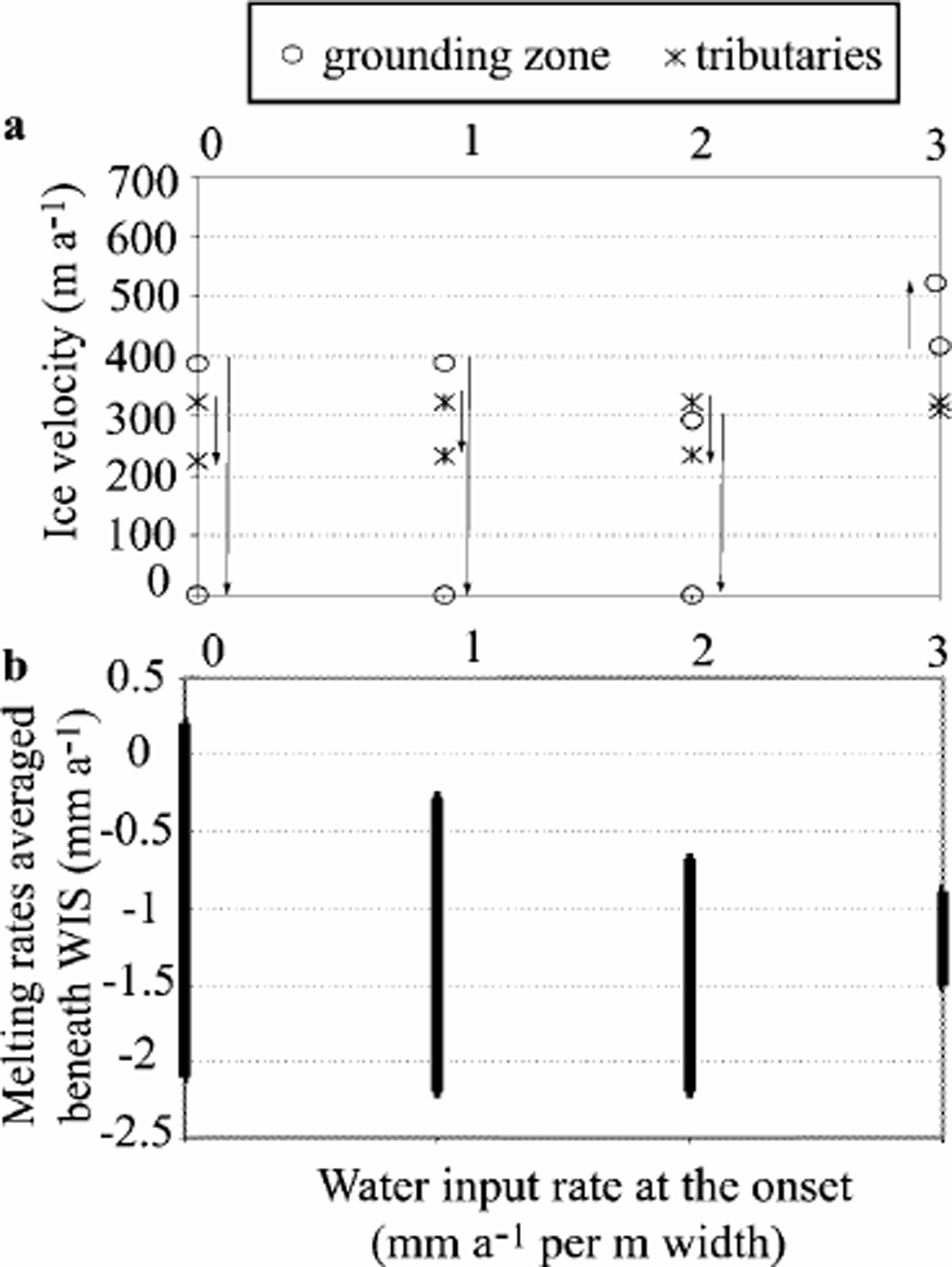
When water-input rates were set to no more than 2 mma–1 per unit bed area (E1–E3), the simulated ice stream experienced a rapid slow-down (within 50 years) followed by a complete shut-down in the grounding-zone area of WIS (Fig. 4a). The stoppage is confined to the lowermost part of the ice stream and does not propagate up to the junction with the tributaries. After WIS stopped, it quickly thickened, particularly at the transition between stagnant and moving ice (Fig. 5). This resulted from the combined effect of accumulation rate, advection of ice from upstream, and transverse influx of ice from ISA and across the lateral shear margins.
Ice thickness along the simulated ice stream 100 years after stoppage, shown here for experiments E1–E3 (modern width, basal water input rate equivalent to 0 mm a–1(dashed line), 1mm a–1(red line) and 2 mm a–1(green line). The initial profile (based on present-day surface map) is plotted in thick solid black, as is the assumed bed topography. This graph illustrates the geometry and position of the ice bump that forms after stoppage. The more drainage, the closer is the grounding line to the ice-bump position, and the less pronounced its shape.

Calculated basal melting/freezing rates were positive beneath the tributaries, where as they remained negative beneath the main trunk (∼–2mma–1 on average in the undrained case; Fig. 4b). Because of the assumed relationship between basal freezing and bed strengthening (Reference S.M., Kamb and EngelhardtTulaczyk and others, 2000b), the computed mean value of ṁ beneath the ice stream is a good predictor of ice-stream stoppage. Indeed, in experiments E1–E3 the spatially averaged basal/freezing rate was below–2mma–1 and it was always able to completely consume the added basal water (Fig. 4b). Hence, freeze-on-driven strengthening commences and then increases with time because of the positive feedback between freezing, shear heating and sliding velocity encapsulated in the bed treatment proposed by Reference S.M., Kamb and EngelhardtTulaczyk and others (2000b).
In experiment E4, the water-input rate equivalent to 3 mm a–1 of melting per unit area of the bed was sufficient to prevent till strengthening and ice-stream slow-down. This rate is high but not unreasonably so, indicating that direct observational constraints on the amount of basal water available beneath WIS may be necessary to reliably predict the near-future evolution of this ice stream. Experiment E4 with the highest basal water input is also the only one in which the predicted velocity never dropped. Perhaps the most important observation is that in all these model runs a velocity slow-down is always a sign of a coming ice-stream stoppage. The ice-stream system, as represented by equations contained in the model, retains the binary nature of the analytical model presented previously by Reference S.M., Kamb and EngelhardtTulaczyk and others (2000b). The simulated ice stream is either able to maintain a non-freezing and non-strengthening bed or it switches to freezing, which triggers a runaway bed strengthening that brings the ice stream to a halt.
4.2. Influence of ice influx from ISA and ISC
In Figure 6a (E5), we show results ofa numerical experiment in which all of the parameters and boundary conditions were kept the same as in the baseline case E1 but the input of ice from ISA was turned off completely. This perturbation allowed propagation of the stoppage somewhat further upstream, by about 50 km. Elimination of ice input from ISA had less impact on the propagation of stoppage if basal water input was included (E6,Table 3).
A time–distance diagram showing the comparison of center-line velocity fields calculated in experiments E5 (a), E1 (b) and E7 (c). The coordinate x = 0 km corresponds to the assumed onset of tributaries, and x = 435 km corresponds to the assumed grounding-line position. The junction between tributaries and main trunk is at x =185 km. Time is displayed on the vertical axis. Contour lines represent ice-flow velocity values (in m a–1). For these experiments, the ice-stream width corresponds to the modern WIS width, and no basal water input is assumed. There is no influx of ice from ISA or ISC in (a). ISA flux is added in (b), and both are added in (c).
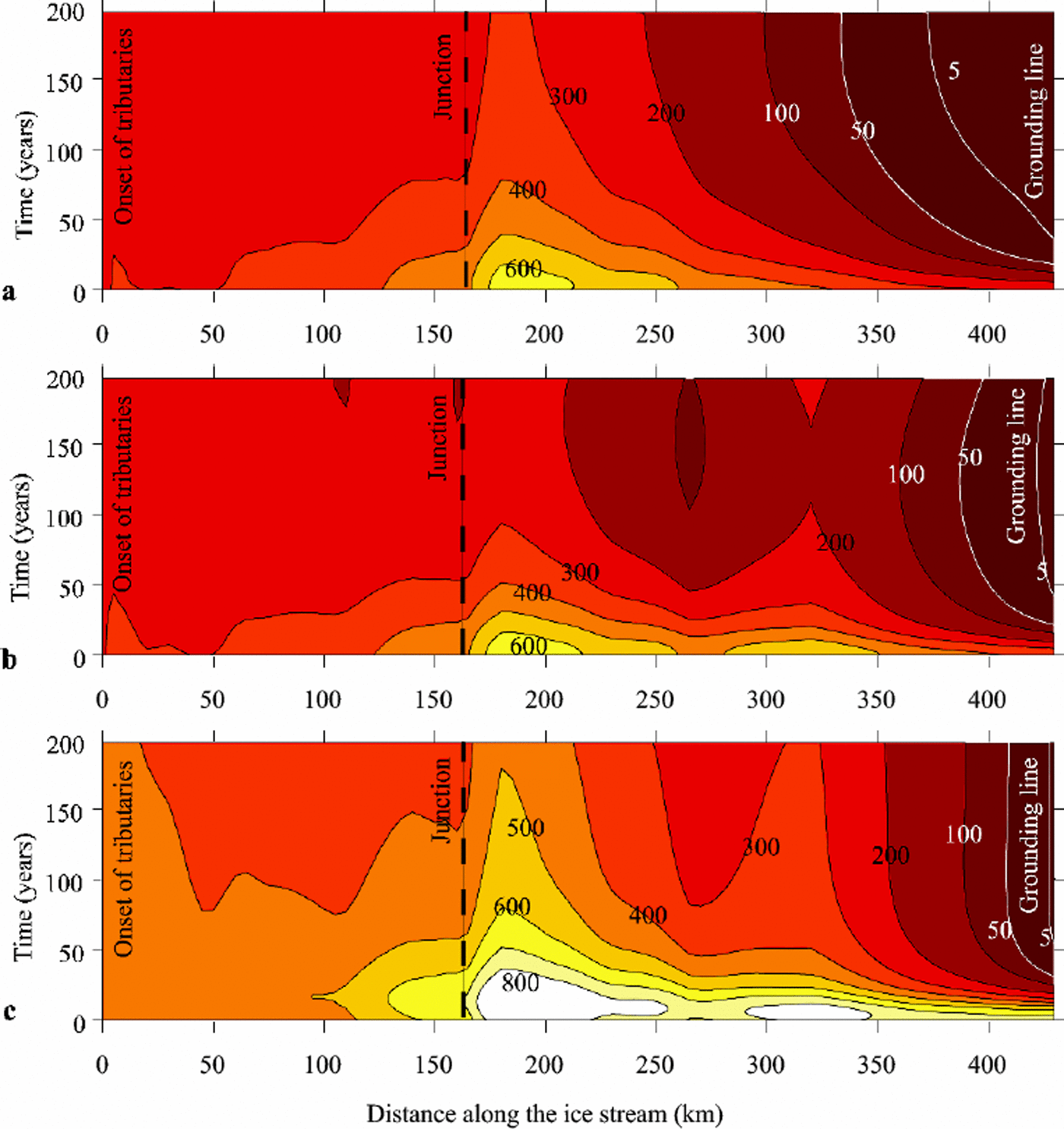
In a separate set of experiments, the impact of possible complete ice diversion from ISC tributaries to WIS was explored (E7, Table 3). This change increased simulated ice velocity by about 30–100% along the whole flowline (Fig. 6c), without preventing slow-down at the grounding zone (basal water input rates rose to 1mm a–1).
4.3. Width changes
Experiments were run with ice-stream width distribution set to be significantly narrower than the modern configuration. Everything else was similar to the experiments described above.
We began by setting the ice-stream maximum width to is be one-third of its actual value (Fig.3b). In this set of experiments, results are similar for cases with and without water velocity input (Fig. 7) because basal freezing never becomes large cases enough to initiate bed strengthening even when no extra basal rate water is added. Consequently, no ice-stream slowdowns or stoppages were observed. With such a narrow ice stream, the ice thickness was greater than the modern one at the end of the model spin-up period and increased further during the actual model run. The large ice thickness induces low basal temperature gradients and hinders basal freezing.
Ice-stream velocity (m a–1) as a function of the assumed ice-stream width for experiments E9–E12. The latter expressed as a fraction of the modern width at the grounding zone. Values represent the maximum and minimum evaluated at x = 435 km (grounding zone). We show two in which we have assumed an equivalent basal water-input of 2mm a–1 (labeled with “*”) and 0 mm a–1 (labeled with “o”). Arrows indicate how the velocity is changing through time.

We also ran a second set of fixed-width experiments, where the maximum ice-stream width was set to be half of the modern value (Fig 3b). Again, thebasalwater-input rate was assumed to be 0 mm a–1 in the first experiment, compared to 2 mm a–1 in the second one. The applied reduction of ice-stream width allows the ice stream to flow continuously with a lower water-input rate than in the modern, wide-ice-stream case (2mm a–1 vs 3 mm a–1).
5. Discussion and Conclusions
Results of our modeling of WIS support the conjecture that the observed recent slow-down of this ice stream may lead to a complete shut-down of the lowermost portion of WIS within the next few decades. We make this statement because all slow-downs produced in our simulations resulted in a complete ice-stream stoppage. We were able to prescribe boundary conditions (e.g. sufficient amount of basal water input) that averted ice-stream stoppage, but in these cases the model did not produce any slow-downs either. Since we obtain a steady velocity field when the sub-ice-stream bed is not strengthening, we do not favor the explanation that the observed slow-down of WIS results from a decrease in driving stress (Reference Joughin, Tulaczyk, Bindschadler and PriceJoughin and others, 2002). One realistic outcome of our model is its ability to produce constant slow-down rates. This feature is consistent with available observations, which indicate that the lower part of WIS was slowing down between 1974 and 1997 at a relatively steady rate of ∼5ma– 2 (Reference Joughin, Tulaczyk and EngelhardtJoughin and others, 2003). Although the simulated linearity of slow-down is realistic, our model does consistently over-predict the rate of slow-down, at ∼15ma–2(Fig. 8). Within the physical framework contained in our model, this unsatisfactory outcome maybe due to either too high calculated basal freezing rates or too sensitive assumed dependence of bed strength on freezing rates. Alternatively, the model may be missing some important physical process/es, which in reality make/s ice streams slow down less rapidly than predicted here.
Changes in center-line velocity at the grounding line over the first 200 model years after the end of the spin-up phase (at 0 years). Several experiments which resulted in a simulated WIS shut-down are shown, plus one experiment (E4) in which shut-down is averted by an injection of basal water at the rate of 3 mm a–1per unit area of the bed.

The model predicts that a relatively large amount of basal water (2 and 3 mm a–1 per unit area of the ice-stream bed) would have to be imported from upstream to avert WIS slow-down and stoppage. Although large, this volume could, however, be delivered by long-distance water drainage from beneath central parts of the ice sheet. This result underscores the need for much better observational constraints on the efficiency and physical nature of sub-ice-stream water drainage.
Based on the model results, we conjecture that neither admissible changes in the overall mass balance of WIS nor any reasonable narrowing of this ice stream can avert its continuing slow-down. Only a transient injection of extra basal water could produce in our model a situation in which the ice stream slows down but never stops.
Acknowledgements
The authors acknowledge financial support from the U.S. National Science Foundation (OPP 9873593 and 0096302) and NASA.We also appreciate reviews of an earlier version of the manuscript by R. C.A. Hindmarsh, K. Hutter and J. Fastook.



