1. Introduction
Rehabilitation therapy aims to restore and regain motor function of the limb after stroke or some other cases like accidents. The hope is that through physical exercises, the patient can recover the lost or weakened function. However, these types of exercises are long-term processes, and conventional rehabilitation is not only time consuming, tedious, and exhausting for the physiotherapist but also imposes a great economic onus on the patient. Rehabilitation robots are presented to overcome these drawbacks of traditional rehabilitation and perform the therapy training more intelligently, accurately, and comfortably. These robots allow intensifying the therapy process by increasing the number of repetitions and the exercise duration without any further physical effort by the expert nor losing the accuracy of the training. Moreover, these robotic systems can acquire and save data during the exercise, like the position, velocity, and interaction torques, for online monitoring and further analysis. Such facilities may not be available in conventional rehabilitation, easily.
Over the last two decades, many lower-limb rehabilitation robotic systems have been developed to aid stroke survivors in performing various styles of rehabilitation exercises, to recover mobility of the limb. These systems can be divided, according to the exercise posture, into two main categories [Reference Wang, Hou, Tong, Zhang, Chen and Tan1]. The first category involves the robots for training in sitting/lying positions. These robots are used in the early stage of therapy where patients cannot stand or walk safely due to high muscle weakness [Reference Farjadian, Nabian, Mavroidis and Holden2, Reference Wang, Feng, Zhang, Chen, Du, Yan and Vladareanu3]. Robots in this category assist the patient in strengthening muscles, developing endurance, and increasing joint mobility and movement coordination. The second category includes the robots for training in walking/standing position, either overground or treadmill [Reference Hussain, Xie and Jamwal4]. The main aim of these robots is to drive the patient’s lower limb, who can stand and has adequate endurance, on a gait trajectory.
The main task of the rehabilitation robotic systems is to move the joints of the injured limb along specific trajectories. To perform this task precisely, various controller approaches have been developed. Proportional integral derivative (PID) controller and its types, PD and PI, are also used in rehabilitation robotic systems. In ref. [Reference Naghavi and Mahjoob5], Naghavi et al. implement a PID control loop to perform trajectory tracking control for a knee rehabilitation robot. A neuromuscular electrical stimulation device is controlled by an adaptive PID controller with an online tuning parameter to perform exercises for the upper limb [Reference Paz, Oliveira, Pino and Fontana6, Reference Roux-Oliveira, Costa, Pino and Paz7]. In ref. [Reference Han, Wang and Tian8], researchers propose an intelligent Proportional-Derivative (PD) controller with a sigmoid function-based tracking differentiator to achieve motion control of a 12-Degree-Of-Freedom (12-DOF) lower-limb exoskeleton robot. Yousefi et al. develop a sliding-backstepping control for a knee rehabilitation robot [Reference Yousefi, Alipour, Tarvirdizadeh and Hadi9]. Riani et al. develop a robust adaptive integral terminal sliding mode control approach, designed to control an upper-limb rehabilitation exoskeleton [Reference Riani, Madani, Benallegue and Djouani10]. Oliviera et al. introduce a robust sliding mode control and implemented it to a neuromuscular electrical stimulation device to achieve a predetermined angular trajectory for the upper limb [Reference Oliveira, Costa, Catunda, Pino, Barbosa and de Souza11]. Neural networks (NNs) models have powerful approximation performance and self-learning ability, which can compensate for the uncertainty of the mathematical model of the robotic systems and handle any external disturbances. Radial basis function (RBF), compared to other types of NNs, for example, Markovian NNs [Reference Li, Li, Zhang, Yang and Gui12], has the best approximation, simple training, fast learning convergence speed, and avoids falling into a local minimum. Moreover, it can improve the real-time tracking performance of the controller [Reference Beyhan and Alcı13, Reference Poultangari, Shahnazi and Sheikhan14]. Thus, it has been widely used in rehabilitation robotic systems controllers. In ref. [Reference Zhang, Zhang and Zhang15], researchers propose an adaptive sliding mode control (ASMC) based on RBF NNs for a lower-limb rehabilitation robot for active therapy sessions. The RBF block is introduced to compensate for external disturbances and uncertainties. Shi et al. [Reference Shi, Xu, Cheng, Xu, Chen and Liang16] develop an RBF-based PID control to achieve the trajectory tracking task of a lower-limb rehabilitation robot.
The safety of the patient during the therapy is a crucial criterion in designing rehabilitation robotic systems. Many studies cover hazards caused by issues such as misalignment when an exoskeleton robot does not align with the human limb properly and exceeds the normal range of motion [Reference Akiyama, Yamada, Ito, Oda, Okamoto and Hara17–Reference Mallat, Khalil, Venture, Bonnet and Mohammed19]. On the contrary, investigation about the safety of rehabilitation robots to handle involuntary movements is limited. Involuntary movements, such as myoclonusFootnote 1 , are common after stroke, due to muscle disorders [Reference Bansil, Prakash, Kaye, Wrigley, Manata, Stevens-Haas and Kurlan20, Reference Alarcón, Zijlmans, Dueñas and Cevallos21]. During the training exercise, these movements may occur and exert interaction torques that lead to substantial injuries or damage to the patient’s limb. Thus, a safe interaction between the patient and the robot is vital [Reference Bessler, Prange-Lasonder, Schaake, Saenz, Bidard, Fassi, Valori, Lassen and Buurke22]. This criterion requires having a compliant behavior of the robot to avoid harming the human (patient). Admittance control is widely implemented in the literature to ensure safe interactions between humans and robots in many applications (medical, industrial, etc.) [Reference Sharkawy, Koustoumpardis and Aspragathos23, Reference Yu and Perrusquía24]. It maps interaction forces/torques into position/velocities, and thus it makes the robot complies with any external forces applied by a human and changes its behavior. In rehabilitation robots, admittance control has been implemented to enable the participation of the patient during the exercise. This participation is mainly required for therapy stages, where the patient can control their limb, but they are still weak to move independently [Reference Ochoa Luna, Rahman, Saad, Archambault and Ferrer25, Reference Taherifar, Vossoughi and Ghafari26].
This research presents a stationary knee rehabilitation robotic system (KRRS), to be used in clinical therapy. KRRS has a new innovative mechanism to measure the interaction torques by load cells. The robot is controlled by the therapist using a user interface (UI), where he/she can monitor the session in real time and save the results for further analysis. A novel admittance proportional-derivative controller augmented by a radial basis function (PD-RBF) control approach is developed for KRRS. This proposed controller consists of two loops, an outer loop and an inner loop. The former has an admittance control algorithm to handle the undesirable interaction torques between the patient’s limb and the robot. The latter achieves the trajectory tracking task. We suggest an RBF NN to augment the conventional PD controller as a feedforward loop. This RBF compensates for the nonlinear characteristics of the system and improves the performance of the PD controller with no need for prior knowledge of the dynamic model of the system. To validate the efficiency of this PD-RBF controller, we consider two controllers, a nonlinear model-based controller, ASMC, and a linear model-free one, PD. Then, we evaluate the proposed PD-RBF by a comparative study among these controllers. The integral absolute error (IAE) and the control effort (CE) are defined as performance indices and analyzed for the mentioned controllers. The main contributions of this paper are:
-
1. Design a new mechanism to measure the interaction torques exerted by the patient’s involuntary movements during the therapy session.
-
2. Propose a new model-free controller to handle these measured torques smoothly and safely.
The remainder of this paper is structured in the following manner. In the next section, the parts of the robot prototype (mechanical components, driver, sensors, etc.) are described. In Section 3, the dynamic model of the robot is extracted. Section 4 includes the design of various control strategies. The experiment results are presented in Section 5. Section 6 includes the results discussion and the comparative study. Finally, the conclusion of this research is abstracted in Section 7.
2. System description
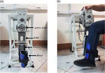
Although determinants of successful lower-limb rehabilitation training robots are unknown, the following properties seem to be important: safety, comfort, accuracy, and ability to perform various types of exercises with desired intensity and number of repetitions. Taking into account the aforementioned properties along with the ease of use by the therapist and low cost, a prototype of KRRS was designed to assist the patient in exercising the knee joint in the sagittal plane. KRRS is designed for the early stages of rehabilitation therapy. It trains the patient’s limb in a sitting position, which is suitable for long-period training sessions, especially for patients not able to stand without assistance/support. Figure 1(a) represents the fabricated prototype of the mentioned robotic system in the ASR Laboratory at the University of Tehran and (b) illustrates how the patient’s leg is attached to the robot.
(a) Prototype of the KRRS; (b) the shank connected to the KRRS.

2.1. System design
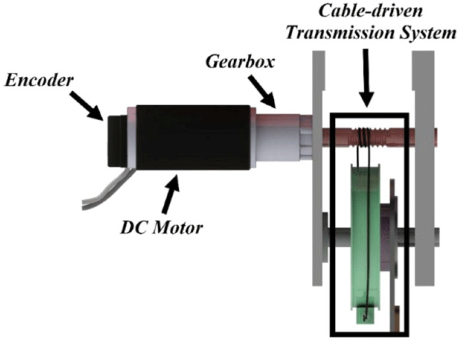
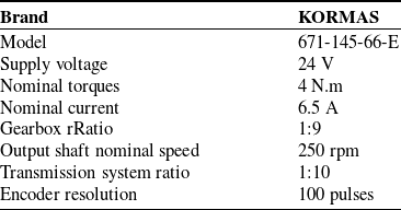
The KRRS mainly consists of a link with a pivot joint that simulates the knee movement. The joint is actuated by a geared DC motor through a cable-driven transmission system. An optical encoder is mounted on the motor shaft to measure the joint position. The motor, transmission system, and encoder are shown in Fig. 2, and their specifications are illustrated in Table 1.
DC motor with transmission system.

The patient’s shank is attached to the link in parallel by a brace, as shown in Fig. 1(b). The length of the link can be adjusted in a range between 45 and 63 cm, with an adjustment step of 1.5 cm. This feature permits the KRRS to fit the various lengths of the patient’s shank.
2.1.1. Involuntary movements measurements mechanism
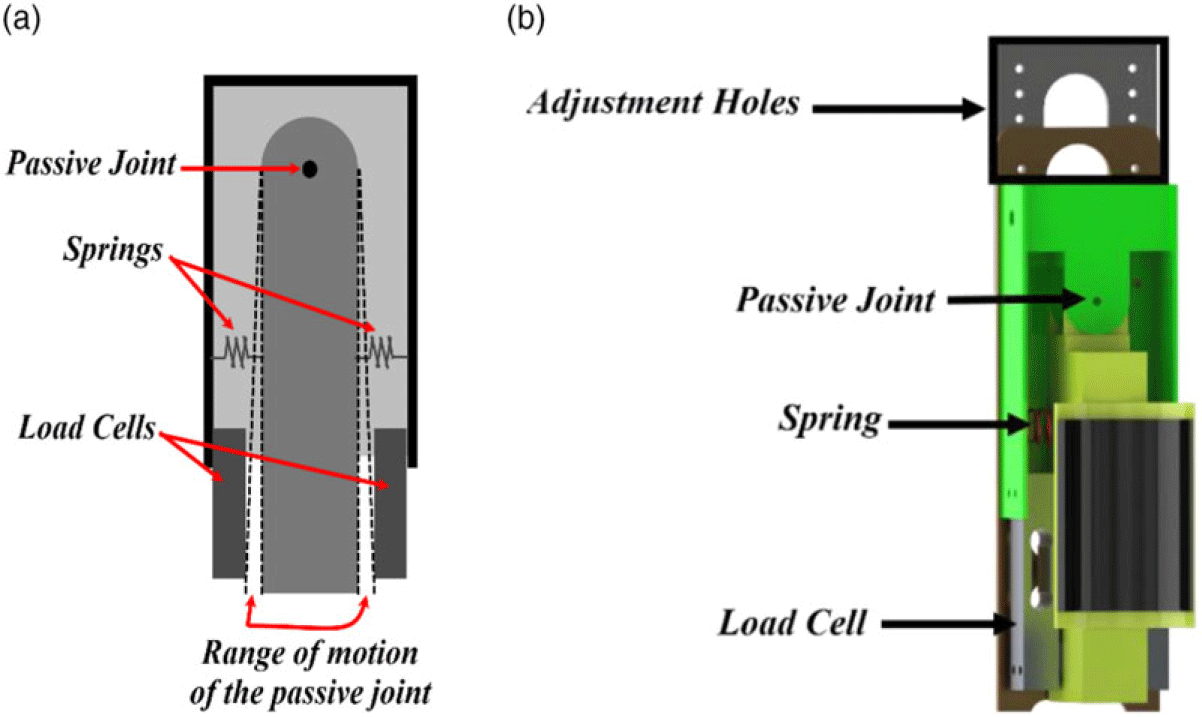
To measure potential involuntary movements of the knee, we developed a new mechanism based on the bar load cells. We used two straight bar load cells, mounted on the link sides. The brace is connected to the KRRS link via a passive joint. Once the knee moves involuntarily, this passive joint allows the brace to move and hit one of the load cells. The motion range of the passive joint is limited, and it is restricted by two high-stiffness springs at each side. Figure 3 represents (a) the schematic and (b) the CAD model of the load cells positions along with the brace, springs, and passive joint.
(a) The schematic and (b) CAD model of the passive joint, brace, springs, and load cells.

2.2. Control unit
Since the proposed KRRS works in direct contact with a human, any delay in the control loop may endanger the patient’s safety. For instance, the delay in acquiring the measured interaction force will lead to mishandle this excessive force and the robot may exceed the predefined limits if there is a delay in reading the actual angular position. Such cases can cause serious harm to the patient’s leg. Thus, it is essential that the control unit should work in real time and avoid any delay in both receiving commands from the physiotherapist and acquiring data from the sensors.
Even PCs provide the ability to design control software easily using high-level programming language environments such as MATLAB and LabVIEW. However, they are not designed to achieve uninterrupted real-time control [Reference Gupta and Sharma27]. They share their resources between the control software and other system activities. Some of these activities are under user control, while some others are not. This affects the speed and repeatability of the operation of the robot and is out of user’s control. Moreover, when a PC freezes or undergoes hard drive failure, due to some of these activities, the I/O unit controlling the robot will not be often neither controllable nor monitored.
Specification of actuating system.

To provide a real-time system, an ARM Cortex-M4-based STM32 microcontroller (model number: STM32F407ZGT6) is utilized as the control unit of KRRS. This microcontroller is programmed by C programming language, and it works on frequency 168 MHz. All control procedures of the robot are implemented by this microcontroller. On the other hand, a host PC is connected to the control unit. Using a UI on this host PC, the therapist can observe the therapy session, as well as command the control unit. Another AVR Atmega328-based board is used for safety, which controls a relay that shuts down the whole system immediately when the emergency pushbutton is pressed.
2.3. User interface
Based on C# programming language, an appropriate and user-friendly UI has been developed. This UI is available as an executable file (*.exe). Thus, it can be installed on any Windows-based PC. By this UI, a physiotherapist can perform the following functions:
-
Send the main commands to the control unit: start, stop, pause, and resume.
-
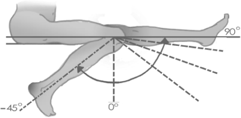
Select the suitable range of motion for the patient within the range of motion of the knee. Figure 4 shows the range of motion of the tibia with respect to the vertical axis according to ref. [Reference Akdoğan, Taçgın and Adli28].
-
Set the exercise mode: passive or active. In both modes, the robot drives the patient’s limb on a reference trajectory. Patients’ interaction forces are not considered in the passive mode. While in the active mode, these interaction forces are measured and considered during the session.
-
Monitor data of the therapy session in real time: these data are divided into two sets:
Range of motion of the knee joint.

The first set of data is for evaluating the therapy progress of the patient: position and interaction torques. The other set is for evaluating the performance of the robot: tracking error, control output, and CE. Moreover, these data can be saved to an Excel file for further analysis.
3. Dynamic model
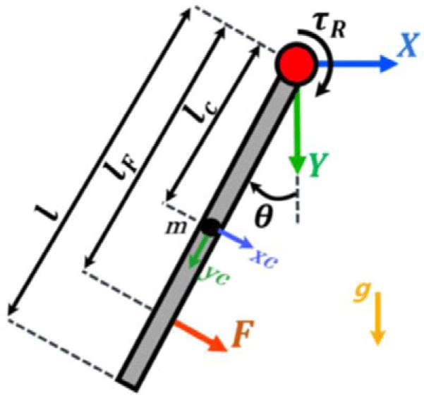
To extract the dynamic model of the system, the schematic of the robot is illustrated in Fig. 5. In this schematic, we did not consider the passive joint as part of the dynamic model due to its significantly low range of motion and low motion frequency; hence, it does not have dynamic behavior. The dynamic model of the robot is obtained using the Euler–Lagrange method as follows:
The schematic of the robot.

The Lagrangian of the KRRS is given by [Reference Morin29]
 \begin{equation}\mathcal{L}=\mathcal{K}-\mathcal{P}\end{equation}
where
 $\mathcal{K}$
and
 $\mathcal{P}$
are the kinetic and potential energies, respectively, given as follows:
 \begin{equation}\mathcal{K}=\frac{1}{2}\left(m\dot{x}_{c}^{2}+m\dot{y}_{c}^{2}+I_{1}\dot{\theta }^{2}\right)\end{equation}
 \begin{equation}\mathcal{P}=-mgy_{c}\end{equation}
where
 $m$
is the mass of the robot arm and
 $g$
is the gravitational acceleration.
 $x_{c}$
and
 $y_{c }$
represent the position of the centroid of the link with respect to the origin of the coordinates system at its joint, which can be obtained as follows:
 \begin{equation}x_{c}=-l_{c}sin\theta\end{equation}
 \begin{equation}y_{c}=l_{c}cos\theta\end{equation}
where
 $l_{c}$
is the distance between the center of mass of the robot arm and the joint and
 $\theta$
and
 $\dot{\theta }$
are the angular position and velocity of the robot joint, respectively.
 $\dot{x}_{c}$
and
 $\dot{y}_{c }$
are velocity of the center of mass of the arm and given as
 \begin{equation}\dot{x}_{c}=-l_{c}\dot{\theta }cos\theta\end{equation}
 \begin{equation}\dot{y}_{c}=-l_{c}\dot{\theta }sin\theta\end{equation}
 $I_{1}$
is the moment of inertia of the robot arm at the joint and given by the parallel axis theorem:
 \begin{equation}I_{1}=I_{c}+ml_{c}^{2}\end{equation}
where
 $I_{c}$
is the moment of inertia of the robot at the center of mass.
Then, the dynamic model is given as follows:
 \begin{equation*}\tau =\frac{d}{dt}\left(\frac{\partial L}{\partial \dot{\theta }}\right)-\left(\frac{\partial L}{\partial \theta }\right)\end{equation*}
 \begin{equation*}=(I_{c}+2ml_{c}^{2})\ddot{\theta }+mgl_{c}sin\theta\end{equation*}
 \begin{equation}=M_{R}\ddot{\theta }+G_{R}\left(\theta \right)\end{equation}
where
 $\ddot{\theta }$
is the angular acceleration of the robot joint.
 $M_{R}$
and
 $G_{R}\left(\theta \right)$
are the nominal inertia and gravity terms, respectively, which are expressed as
 \begin{equation}M_{R}=I_{c}+ml_{c}^{2}\end{equation}
 \begin{equation}G_{R}\left(\theta \right)=mgl_{c}cos\theta\end{equation}
 $\tau$
is the external torque applied on the robot arm, and it is obtained as follows:
 \begin{equation}\tau =\tau _{R}-\tau _{int}\end{equation}
where
 $\tau _{R}$
is the actuator torque and
 $\tau _{int}$
is the interaction torque between the robot and the patient’s leg which can be derived as follows:
 \begin{equation}\tau _{int}=Fl_{F}\end{equation}
where
 $F$
denotes the interaction force between the robot and the patient, excluding the weight, inertia, and other elastic/viscoelastic torques in the knee joint, which is the force exerted by the leg and measured by the load cells.
 $l_{F}$
is the distance between the load cell and the robot joint, as shown in Fig. 6.
Block diagram of the ASMC.

In practice, the nominal values of the dynamic model of the robot do not represent the real dynamic behavior of the system, due to many factors. These factors are either unknown, like system uncertainties and external disturbances, or difficult to compute accurately, like patient’s leg. A new term,
 $D(t)$
, is defined that includes all unknown factors, where
 $D\left(t\right)$
is assumed to be unknown, but bounded. Thus, the dynamic model of the KRRS is given as follows:
 \begin{equation}\tau -\tau _{int}=M_{R}\ddot{\theta }+G_{R}\left(\theta \right)+D(t)\end{equation}
Then the angular acceleration of the robot joint will be as follows:
 \begin{equation}\ddot{\theta }=M_{R}^{-1}\left\{\tau -\tau _{int}-G\left(\theta \right)-D(t)\right\}\end{equation}
4. Control design
In the KRRS, we develop the control algorithm to fulfill the following objectives: (a) perform an accurate trajectory tracking task and (b) handle the measured interaction torques exerted by the patient safely and appropriately.
To realize these objectives, a control algorithm consists of two loops: the outer control loop and the inner control loop. Both of these loops are implemented in the control unit (STM32 board). The functionality of these loops is explained as follows.
4.1. The outer control loop
During the exercise session by the KRRS, the patient’s limb may move either voluntarily by the patient or involuntary because of a neurological disorder. This movement generates an interaction torque. This torque is undesirable and may cause pain or injury for the patient. To reduce the effects of these interaction torques and avoid secondary injury, we implement an admittance (reverse impedance) control strategy. The undesirable interaction torques are measured by load cells. Then, they are applied to the input of admittance control. The admittance control attains the flexibility of the robot by changing its trajectory suitably according to the measured torques.
Using a mass-damper-spring impedance model [Reference Song, Yu and Zhang30], the interaction torque can be given as follows:
 \begin{equation}M_{i}\ddot{\tilde{\theta }}+C_{i}\dot{\tilde{\theta }}+K_{i}\tilde{\theta }=\tau _{int}\end{equation}
 \begin{equation}\tilde{\theta }=\theta _{des}-\theta _{r}\end{equation}
where
 $M_{i}, C_{i}, K_{i}$
are the inertia, damping, and stiffness impedance terms, respectively. These terms should be chosen in a way that ensures a smooth and safe change in the reference trajectory.
 $\theta _{des}$
is the predefined trajectory and
 $\theta _{r}$
is the reference trajectory, which is the input of the inner control loop.
 $\tilde{\theta }$
is the robot trajectory deviation from the predefined trajectory.
 $\tau _{int}$
is the undesirable interaction torque. When
 $\tau _{int}=0$
, we have
 $\tilde{\theta }=0$
and
 $\theta _{r}=\theta _{des}$
, and when the interaction torque is exerted, the reference trajectory changes and deviates from the predefined trajectory. Substituting Eq. (17) in (16), the reference trajectory, which is proper to the exerted interaction torques, can be obtained as follows:
 \begin{equation}M_{i}\left(\ddot{\theta }_{des}-\ddot{\theta }_{r}\right)+C_{i}\left(\dot{\theta }_{des}-\dot{\theta }_{r}\right)+K_{i}\left(\theta _{des}-\theta _{r}\right)=\tau _{int}\end{equation}
 \begin{equation}\ddot{\theta }_{r}=\ddot{\theta }_{des}-M_{i}^{-1}\left\{C_{i}\left(\dot{\theta }_{des}-\dot{\theta }_{r}\right)+K_{i}\left(\theta _{des}-\theta _{r}\right)-\tau _{int}\right\}\end{equation}
4.2. The inner control loop
This loop achieves the trajectory tracking task, where the robot guides the leg to move along a reference trajectory with the highest possible accuracy. The tracking error, which is the difference between the reference angular position
 $(\theta _{r})$
and the robot actual angular position
 $(\theta )$
, and its first derivative are given as follows:
 \begin{equation}e=\theta _{r}-\theta\end{equation}
 \begin{equation}\dot{e}=\dot{\theta }_{r}-\dot{\theta }\end{equation}
A PD-RBF NN is proposed to be applied in this loop. However, before discussing the aforementioned proposed approach, two other controllers are introduced for a comparative study purpose: an ASMC, as a representation of the model-based controller, and a conventional PD controller, as a model-free controller. The results of these controllers are used in a comparative study to prove the efficiency of the PD-RBF controller. The reasons behind choosing these two controllers, PD and ASMC, are
-
PD, as a variation of PID, is the most basic and simplest controller for any system and one of the most widely used controllers for robots in trajectory tracking tasks. However, its performance is subject to the nonlinearity level of the system [Reference Feng, Yin, Weng, Ma, Zhou, Jia and Zhang31]. Therefore, since our system is nonlinear, we start from PD and seek to improve its performance for our system. Then validate the improved PD (PD-RBF) by comparing its performance with the conventional PD.
-
Sliding mode control (SMC) has a robust property and a complex structure, which is commonly used to control nonlinear systems with known uncertain bounds [Reference Shtessel, Edwards, Fridman and Levant32]. ASMC is an improved version of SMC to control nonlinear systems when the boundaries of the uncertainty are unknown, which is more practical [Reference Roy, Baldi and Fridman33]. Thus, since the proposed PD-RBF is an advanced control, it is reasonable to examine its performance with a controller more complex than PD, such as ASMC, to have fair comparison.
4.2.1. Adaptive sliding mode control
In rehabilitation robots, many control methodologies based on SMC have been developed [Reference Yousefi, Alipour, Tarvirdizadeh and Hadi9, Reference Babaiasl34–Reference Torabi, Sharifi and Vossoughi36]. In this research, an ASMC with PID surface has been introduced to perform trajectory tracking control.
The sliding surface can be defined as follows [Reference Eker37]:
 \begin{equation}s=\dot{e}+\beta _{1}e+\beta _{2}\int edt\end{equation}
where
 $\beta _{1}$
and
 $\beta _{2}$
are positive gains.
The aim of the SMC is to force the error to approach the sliding surface and then move the error along the sliding surface toward the zero.
To achieve this aim, the control law of SMC should be designed in a way that the following expression is maintained:
 \begin{equation}\dot{s}=0\end{equation}
This condition is necessary to ensure that the error stays on the sliding surface.
where
 $\dot{s}$
is the time derivative of the sliding surface and derived as follows:
 \begin{align}\dot{s}&=\ddot{e}+\beta _{1}\dot{e}+\beta _{2}e\\[5pt] & =\left(\ddot{\theta }_{r}-\ddot{\theta }\right)+\beta _{1}\dot{e}+\beta _{2}e \nonumber \end{align}
Substituting (15) in (24) yields:
 \begin{equation}\dot{s}=\left(\ddot{\theta }_{r}-M_{R}^{-1}\left\{\tau -\tau _{int}-G\left(\theta \right)-D(t)\right\}\right)+\beta _{1}\dot{e}+\beta _{2}e\end{equation}
Equation (25) has known (nominal and measurable) and unknown, but bounded, terms. Herein, we introduce a control law that consists of two terms, an equivalent and auxiliary, the former considers the known term while the latter tries to vanish the impact of the unknown term. The control law is
 \begin{equation}\tau =\tau _{eq}+\tau _{aux }\end{equation}
making
 $\dot{s}=0$
, and neglecting the unknown term
 $D(t)$
, the equivalent control law
 $\tau _{eq}$
is obtained as
 \begin{equation}\tau _{eq}=M_{R}\left(\ddot{\theta }_{r}+\beta _{1}\dot{e}+\beta _{2}e\right)+G_{R}\left(\theta \right)+\tau _{int}\end{equation}
The term of system uncertainties and disturbance (
 $D(t)$
) leads the tracking error to drift away from the sliding surface. In order to overcome this issue, an auxiliary control law is defined. This auxiliary control law has a switching discontinuous function which forces the tracking error to lie on the sliding surface. The auxiliary control law
 $\tau _{aux}$
is given as:
 \begin{equation}\tau _{aux}=M_{R}\left(K_{1}s+K_{2}sign\left(s\right)\right)\end{equation}
where
 $K_{1}$
and
 $K_{2}$
are positive gains. The sign function,
 $sign(\blacksquare )$
, is the ideal discontinuous function, which guarantees an infinitely fast switching. However, in practice, it is impossible to achieve infinitely fast switching control because of the finite time delays for the control computation and limitations of the physical actuators. This imperfect switching in practice raises the oscillation problem, known as chattering. Chattering is a harmful phenomenon because it leads to low control accuracy, may damage the physical parts of the system, and requires lots of energy for good efficiency. A common method to reduce chattering is to define a boundary layer near the sliding surface and then use a saturation function instead of the sign function. When the system is within the boundary layer, a continuous control will be achieved and the chattering will be alleviated. The saturation function
 $sat(\blacksquare )$
is defined as follows:
 \begin{equation}sat\left(s\right)=\begin{cases} \varphi & s\geq \varphi \\ -\varphi & s\leq \varphi \\ s & -\varphi \lt s\lt \varphi \end{cases}\end{equation}
where
 $\varphi$
is the boundary layer thickness.
Thus,
 $\tau _{aux}$
will be
 \begin{equation}\tau _{aux}=M_{R}\left(K_{1}s+K_{2}sat\left(s\right)\right)\end{equation}
Further, in order to improve the robustness of the SMC law, an adaptive term has been introduced.
Assumption 1:
The term
 $D(t)$
is unknown but bounded, that is,
 $\Lambda \gt \left| D(t)\right|$
, where
 $\Lambda$
is unknown positive number. Thus,
 $\hat{\Lambda}$
is the estimated value of
 $\Lambda$
and obtained from the adaptation law:
 \begin{equation}\dot{\hat{\Lambda }}=\kappa \left| s\right|\end{equation}
where
 $\kappa$
is a positive number.
 $\hat{\Lambda }$
is added to
 $\tau _{aux}$
as follows:
 \begin{equation}\tau _{aux}=K_{1}s+K_{2}sat\left(s\right)+\hat{\Lambda }sat\left(s\right)\end{equation}
Finally, by substituting (27) and (32) in (26), the ASMC law,
 $\tau _{ASMC}$
, is given as
 \begin{equation}\tau _{ASMC}=M_{R}\left(\ddot{\theta }_{r}+\beta _{1}\dot{e}+\beta _{2}e\right)+G_{R}\left(\theta \right)+\tau _{int}+K_{1}s+K_{2}\mathrm{sat}\left(s\right)+\hat{\Lambda }sat\left(s\right)\end{equation}
Figure 6 presents the block diagram of the admittance ASMC approach.
Stability analysis
To ensure the stability of the designed controller, a candidate Lyapunov positive definite function
 $V$
is defined as follows:
 \begin{equation}V=\frac{1}{2}\kappa M_{R}s^{2}+\tilde{\Lambda }^{2}\end{equation}
where
 \begin{equation}\tilde{\Lambda }=\Lambda -\hat{\Lambda }\end{equation}
Assumption 2:
Assigning the initial value of
 $\hat{\Lambda }$
as
 $\hat{\Lambda }_{\textbf{0}}\ll \Lambda$
, where
 $\hat{\Lambda }_{\textbf{0}}$
is the value of
 $\hat{\Lambda }$
at t = 0, and for a relatively small value of
 $\kappa$
in Eq. (31),
 $\hat{\Lambda }$
will increase slowly. Moreover, as much as the sliding surface
 $s$
converges to zero,
 $\dot{\hat{\Lambda }}$
converges to zero. This will ensure that
 $\hat{\Lambda }$
will flatten quickly and will not exceed
 $\Lambda$
. Thus, the value of
 $\tilde{\Lambda }$
will be
 $\geq 0$
. Generally, it is guaranteed that
 $\tilde{\Lambda }$
is positive, always.
The derivative of Lyapunov function is given as follows:
 \begin{equation}\dot{V}=\kappa M_{R}s\dot{s}-2(\Lambda -\hat{\Lambda })\dot{\hat{\Lambda }}\end{equation}
Substituting (33), in (25), and, substituting the obtained formula and (31) in (36) lead to:
 \begin{align} \dot{V}& =\kappa s\left(-K_{1}s-K_{2}sat\left(s\right)-\hat{\Lambda }sat\left(s\right)+(D(t)\right)-2(\Lambda -\hat{\Lambda })\kappa \left| s\right| \nonumber \\ & =-\kappa K_{1}s^{2}-\kappa sK_{2}sat\left(s\right)-\kappa s\hat{\Lambda }sat\left(s\right)+\kappa s(D(t)-2(\hat{\Lambda }-\Lambda )\kappa \left| s\right| \nonumber \\ & \quad \leq -\hat{\Lambda }\kappa \left| s\right| +\left| (D(t)\right| \kappa \left| s\right| -2\left(\Lambda -\hat{\Lambda }\right)\kappa \left| s\right| +\Lambda \left| s\right| -\Lambda \left| s\right|\end{align}
Thus, the first derivative of Lyapunov function
 $\dot{V}$
can be written as follows:
 \begin{equation}\dot{V}\leq -\left(\Lambda -\left| (D(t)\right| \right)\kappa \left| s\right| -\left(\Lambda -\hat{\Lambda }\right)\kappa \left| s\right|\end{equation}
Since
 $\left| D(t)\right| \lt \Lambda$
, according to the assumption 1, and by choosing
 $\hat{\Lambda }_{0}$
and
 $\kappa$
properly (based on assumption 2), that provide the condition
 $\tilde{\Lambda }\geq 0$
,
 $\dot{V}$
is negative definite, and according to the global stability theorem of Lyapunov, the stability of the system is guaranteed.
4.2.2. PD controller:
PID controller and its other types, PD and PI, are model-free controller where they do not require any knowledge about the dynamic system. These controllers are widely used for controlling both linear and nonlinear systems due to their simple structure, robustness, ease of implementation, low cost, and high performance [Reference Feng, Yin, Weng, Ma, Zhou, Jia and Zhang31, Reference Kara and Mary38, Reference Sharkawy and Koustoumpardis39]. The PD equation used in this research is described as follows:
 \begin{equation}\tau _{pd}=K_{p}e+K_{d}\dot{e}\end{equation}
The total torque to be applied on the robot is
 \begin{equation}\tau =\tau _{pd}+\tau _{int}\end{equation}
where
 $K_{p}$
and
 $K_{d}$
are the positive proportional and derivative gains, respectively.
 $\tau _{pd }$
is the PD controller output. Figure 7 shows the block diagram of PD controller.
Block diagram of the PD controller.

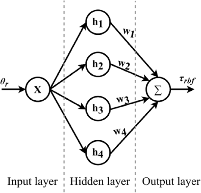
The architecture of the RBF neural network.

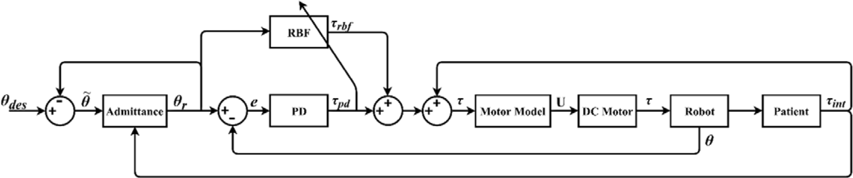
Block diagram of the PD-RBF controller.

4.2.3. PD augmented by RBF
Since the patient’s limb is connected directly to the robot in parallel and the physical characteristics of the leg differ from one patient to another, the nonlinear characteristics of the robot vary dramatically for each patient. This change in the characteristics makes obtaining the accurate dynamic model difficult and affects the performance of the tracking control due to the high nonlinearity. To overcome this problem and provide the KRRS with highly precise tracking performance, we propose a PD controller augmented by an RBF NN block as feedforward loop. The aim of this feedforward loop is to compensate for the nonlinearity terms in the system and improve the tracking accuracy of the model-free controller (PD). RBF is widely implemented to approximate the nonlinearity due to its simplicity and fast convergence [Reference Nguyen, Lin, Su and Tran40, Reference Li and Tian41]. Figure 8 shows the architecture of the proposed RBF NN, which consists of an input layer, hidden layer, and output layer. Gaussian functions are used as an RBF in the hidden layer. Then, the output of RBF,
 $\tau _{rbf }$
, is obtained as follows:
 \begin{equation}h_{i}=\exp \left(-\frac{\left\| X-c_{i}\right\| ^{2}}{2b_{i}^{2}}\right)\end{equation}
where
 $i=1,\ldots,4$
is the number of the neuron and
 $h_{i}$
,
 $c_{i}$
,
 $b_{i}$
are the Gaussian function, center value, and the width values of the neuron
 $i$
, respectively.
 $X$
is the reference trajectory
 $\theta _{r}$
.
And the output of the RBF NN is given as follows:
 \begin{equation}\tau _{rbf}=\boldsymbol{{w}}^{\mathrm{T}}\boldsymbol{{h}}\boldsymbol{{sat}}\left(\tau _{pd}\right)\end{equation}
where
 $\boldsymbol{{w}}\in \mathcal{R}^{4\times 1}$
is the weights vector.
Defining the weights adaptive law as follows:
 \begin{equation}\dot{\boldsymbol{{w}}}=\frac{1}{2}\textbf{P}\,\boldsymbol{{h}}\left| \tau _{pd}\right|\end{equation}
where
 $\textbf{P}\in \mathcal{R}^{4\times 4}$
is a positive diagonal matrix.
Thus, the proposed control output, shown in Fig. 9, is given as follows:
 \begin{equation}\tau =\tau _{rbf}+\tau _{pd}+\tau _{int}\end{equation}
Stability analysis
To analyze the stability of the proposed control strategy, the following assumptions are considered, without any lake of generality:
Assumptions 3:
Define a new term includes the nonlinear and unknown terms of Eq. (15), this new term is unknown but bounded.
 \begin{equation}\Pi(\theta,t)=G\left(\theta \right)+D(t)\end{equation}
The ideal approximation of the NN output
 ${\boldsymbol{{w}}^{*}}^{\mathrm{T}}\boldsymbol{{h}}$
, that is,
 ${\boldsymbol{{w}}^{*}}^{\mathrm{T}}\boldsymbol{{h}}\gt \left| \Pi (\theta,t)\right|$
where
 $\boldsymbol{{w}}^{\boldsymbol{*}}$
denotes the best approximation of the NN weights.
Assumptions 4:
 $K_{p}$
and
 $K_{d}$
are chosen to ensure that the following inequalities are true:
 \begin{equation}2K_{p}K_{d}\gt M_{R}K_{d}^{-1}K_{p}^{2}\end{equation}
 \begin{equation}K_{d}^{2}\gt M_{R}K_{p}\end{equation}
Rewriting the dynamic Eq. (15) as function of error and substituting Eqs. (45), (44), (42), and (39) in it as follows:
 \begin{equation}M_{R}\ddot{e}+K_{d}\dot{e}+K_{p}\mathrm{e}+\boldsymbol{{w}}^{\mathrm{T}}\boldsymbol{{h}}\mathrm{sat}\left(\tau _{pd}\right)-\Pi \left(t\right)=0\end{equation}
Defining the Lyapunov candidate as follows:
 \begin{equation}V=\frac{1}{2}M_{R}K_{d}^{-1}\left(K_{p}e+K_{d}\dot{e}\right)^{2}+\frac{1}{2}\left(2K_{p}K_{d}-M_{R}K_{d}^{-1}K_{p}^{2}\right)e^{2}+2\tilde{\boldsymbol{{w}}}^{\mathrm{T}}\tilde{\boldsymbol{{w}}}\end{equation}
where
 \begin{equation}\tilde{\boldsymbol{{w}}}=\boldsymbol{{w}}^{\boldsymbol{*}}-\boldsymbol{{w}}\end{equation}
Assumption 5:
Assigning the initial value of
 $\boldsymbol{{w}}$
as
 $\boldsymbol{{w}}_{\textbf{0}}\ll \boldsymbol{{w}}^{\boldsymbol{*}}$
, where
 $\boldsymbol{{w}}_{\textbf{0}}$
is the value of
 $\boldsymbol{{w}}$
at t = 0, and for a relatively small values of
 $\textbf{P }$
in Eq. (43),
 $\boldsymbol{{w}}$
will increase slowly. Moreover, as much as the error converges to zero,
 $\dot{\boldsymbol{{w}}}$
converges to zero. This will ensure that
 $\boldsymbol{{w}}$
will be flatten quickly and will not exceed
 $\boldsymbol{{w}}^{\boldsymbol{*}}$
. Thus, the value of
 $\tilde{\boldsymbol{{w}}}$
will be
 $\geq \textbf{0}$
. Generally, it is guaranteed that
 $\tilde{\boldsymbol{{w}}}$
is positive, always.
Differentiating (49), we obtain the following relation for
 $\dot{V}$
.
 \begin{align}\dot{V}&=\left(K_{p}e+K_{d}\dot{e}\right)\left(M_{R}K_{d}^{-1}K_{p}\dot{e}+M_{R}\ddot{e}\right)+\left(2K_{p}K_{d}-M_{R}K_{d}^{-1}K_{p}^{2}\right)e\dot{e}-4\tilde{\boldsymbol{{w}}}^{\mathrm{T}}\dot{\boldsymbol{{w}}}\\[5pt] & = M_{R}K_{d}^{-1}K_{p}^{2}e\dot{e}+M_{R}K_{p}e\ddot{e}+M_{R}K_{p}\dot{e}^{2}+M_{R}K_{d}\dot{e}\ddot{e}+\left(2K_{p}K_{d}-M_{R}K_{d}^{-1}K_{p}^{2}\right)e\dot{e}-2\tilde{\boldsymbol{{w}}}\textbf{P}\boldsymbol{{h}}\left| \tau _{pd}\right| \nonumber \end{align}
Substituting (48) and (43) in (51):
 \begin{align}\dot{V}&=M_{R}K_{d}^{-1}K_{p}^{2}e\dot{e}+\left(K_{p}e+K_{d}\dot{e}\right)\left(-K_{p}e-K_{d}\dot{e}-\boldsymbol{{w}}^{\mathrm{T}}\boldsymbol{{h}}\mathrm{sat}\left(\tau _{pd}\right)+\Pi \left(t\right)\right)+M_{R}K_{p}\dot{e}^{2} \\ &\quad +\left(2K_{p}K_{d}-M_{R}K_{d}^{-1}K_{p}^{2}\right)e\dot{e}-2\tilde{\boldsymbol{{w}}}^{\mathrm{T}}\textbf{P }\boldsymbol{{h}}\left| \tau _{pd}\right| \nonumber \end{align}
Then, the derivative of the Lyapunov function can be written as follows:
 \begin{align} \dot{V}& =-K_{p}^{2}e^{2}-\left(K_{d}^{2}-M_{R}K_{p}\right)\dot{e}^{2}-\boldsymbol{{w}}^{\mathrm{T}}\boldsymbol{{h}}\mathrm{sat}\left(\tau _{pd}\right)\tau _{pd}+\Pi \left(t\right)\tau _{pd}-2\tilde{\boldsymbol{{w}}}^{\mathrm{T}}\textbf{P }\boldsymbol{{h}}\left| \tau _{pd}\right| \nonumber \\[5pt] & =-K_{p}^{2}e^{2}-\left(K_{d}^{2}-M_{R}K_{p}\right)\dot{e}^{2}-\boldsymbol{{w}}^{\mathrm{T}}\boldsymbol{{h}}\left| \tau _{pd}\right| +\Pi \left(t\right)\tau _{pd}-2\tilde{\boldsymbol{{w}}}^{\mathrm{T}}\textbf{P }\boldsymbol{{h}}\left| \tau _{pd}\right| +{\boldsymbol{{w}}^{\boldsymbol{*}}}^{\mathrm{T}}\textbf{P}\boldsymbol{{h}}\left| \tau _{pd}\right| -{\boldsymbol{{w}}^{\boldsymbol{*}}}^{\mathrm{T}}\textbf{P}\boldsymbol{{h}}\left| \tau _{pd}\right| \nonumber \\[5pt] & =-K_{p}^{2}e^{2}-\left(K_{d}^{2}-M_{R}K_{p}\right)\dot{e}^{2}-\left({\boldsymbol{{w}}^{\boldsymbol{*}}}^{\mathrm{T}}\textbf{P}\boldsymbol{{h}}-\left| \Pi \left(t\right)\right| \right)\left| \tau _{pd}\right| -\tilde{\boldsymbol{{w}}}^{\mathrm{T}}\textbf{P }\boldsymbol{{h}}\left| \tau _{pd}\right|\end{align}
 \begin{equation}\dot{V}\leq -\left(K_{d}^{2}-M_{R}K_{p}\right)\dot{e}^{2}-\left({\boldsymbol{{w}}^{\boldsymbol{*}}}^{\mathrm{T}}\textbf{P}\boldsymbol{{h}}-\left| \Pi \left(t\right)\right| \right)\left| \tau _{pd}\right| -\tilde{\boldsymbol{{w}}}^{\mathrm{T}}\textbf{P }\boldsymbol{{h}}\left| \tau _{pd}\right|\end{equation}
Considering assumptions 3, 4, and 5 stated earlier, it can be seen that
 $\dot{V}$
is negative definite, and the system is stable.
5. Experiment results
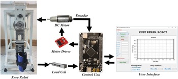
To evaluate the designed controllers, several experiments and tests were performed in the passive mode, where the robot drives the patient’s leg without consideration to any interaction torques, and in the active mode, where the undesirable interaction torques are taken into account. Figure 10 shows a diagram of all parts of the proposed KRRS. The controller program in the experimental environment is written in ARM-based STM32 board in C. The control loop sample time is 20 ms. The 100-pulse encoder is mounted at the motor shaft; the transmission system ratio is 1:90 (1:9 head gearbox, 1:10 cable-driven system); thus, the control resolution is 0.04 degree/pulse (
 $\frac{360}{\text{encoder pulses }(100)}\times \text{transmission system ratio }(1\colon 90)$
). Table 2 shows the characteristics of the equipped load cells. Two 50 kg straight bar load cells are utilized in the system. The safety precautions have been implemented in the KRRS on three levels of mechanical, electrical, and software. Mechanical constraints are added to restrict the robot arm exceeding the range of motion of the knee joint. An emergency button immediately shuts the system down, once it is pressed by the observer or the patient. Joint limits conditions are also considered in the software design to keep the robot arm in the appropriate range of motion. Besides, the observer can stop the robot instantly from the UI.
Diagram of the various parts of the KRRS.

In this section, the results of three experiments, passive with no load, passive loaded, and active loaded, are discussed. The IAE and the CE are defined as the performance indices to analyze the performance of the designed controllers. IAE and CE are given by:
 \begin{equation}IAE=\int \left| e\right| dt\end{equation}
 \begin{equation}CE=\int \left| \tau \right| dt\end{equation}
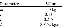
Table 3 shows the admittance parameters and the gains of the ASMC, PD, and PD-RBF. The KRRS parameters used are illustrated in Table 4.
The load cell specifications.

The various controllers parameters.

KRRS parameters.

Remark: The admittance control parameters were experimentally tuned to have a smooth change in the trajectory. The gains of ASMC, PD, and RBF-PD controllers are also experimentally selected considering the IAE and CE indices, where the chosen gains of each controller are the ones that offer a low IAE for an appropriate CE value. It is worth to mention that various tests have conducted to choose the appropriate parameters of the mentioned controllers. For each controller, the best parameters have selected and the related results have reported.
The supply source used for the KRRS is DC voltage source; thus, using the motor dynamic, the obtained torque
 $\tau$
from the controllers is converted to voltage and applied to the DC motor by the control unit to the motor driver as PWM signals.
The motor equations are
 \begin{equation}\tau _{m}=\frac{\tau }{k_{g}}\end{equation}
 \begin{equation}i=\frac{\tau _{m}}{k_{m}}\end{equation}
 \begin{equation}\mathrm{U}=Ri+L\frac{di}{dt}+k_{v}\omega ~\end{equation}
where
 $\tau _{m}$
is the motor torque,
 $k_{g}=1\colon 90$
is the transmission system ratio,
 $k_{m}$
and
 $k_{v}$
are the motor torque and velocity constants, respectively.
 $i$
and
 $U$
are the motor current and voltage, respectively.
 $R$
is the motor resistance,
 $L$
is the inductance, and
 $\omega$
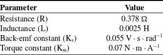
is the motor speed. The physical parameters of the utilized DC motor in the KRRS are obtained using the system identification algorithms. Initially, a persistently exciting pseudo-random binary sequence is applied to the DC motor as input signal, and the shaft speed is measured. These input and output sequences are saved. Then, an appropriate structure of model is considered as the motor model. Finally, the system identification algorithms are utilized to estimate the parameters of the considered model using acquired input/output data [Reference Ljung42, Reference Nelles43]. Several estimation processes are carried out to obtain the most accurate values of these parameters. Table 5 illustrates the estimated values of motor parameters.
DC motor parameters.

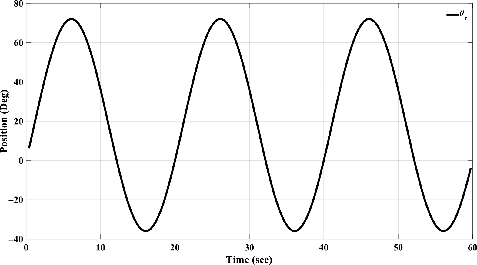
The predefined trajectory.

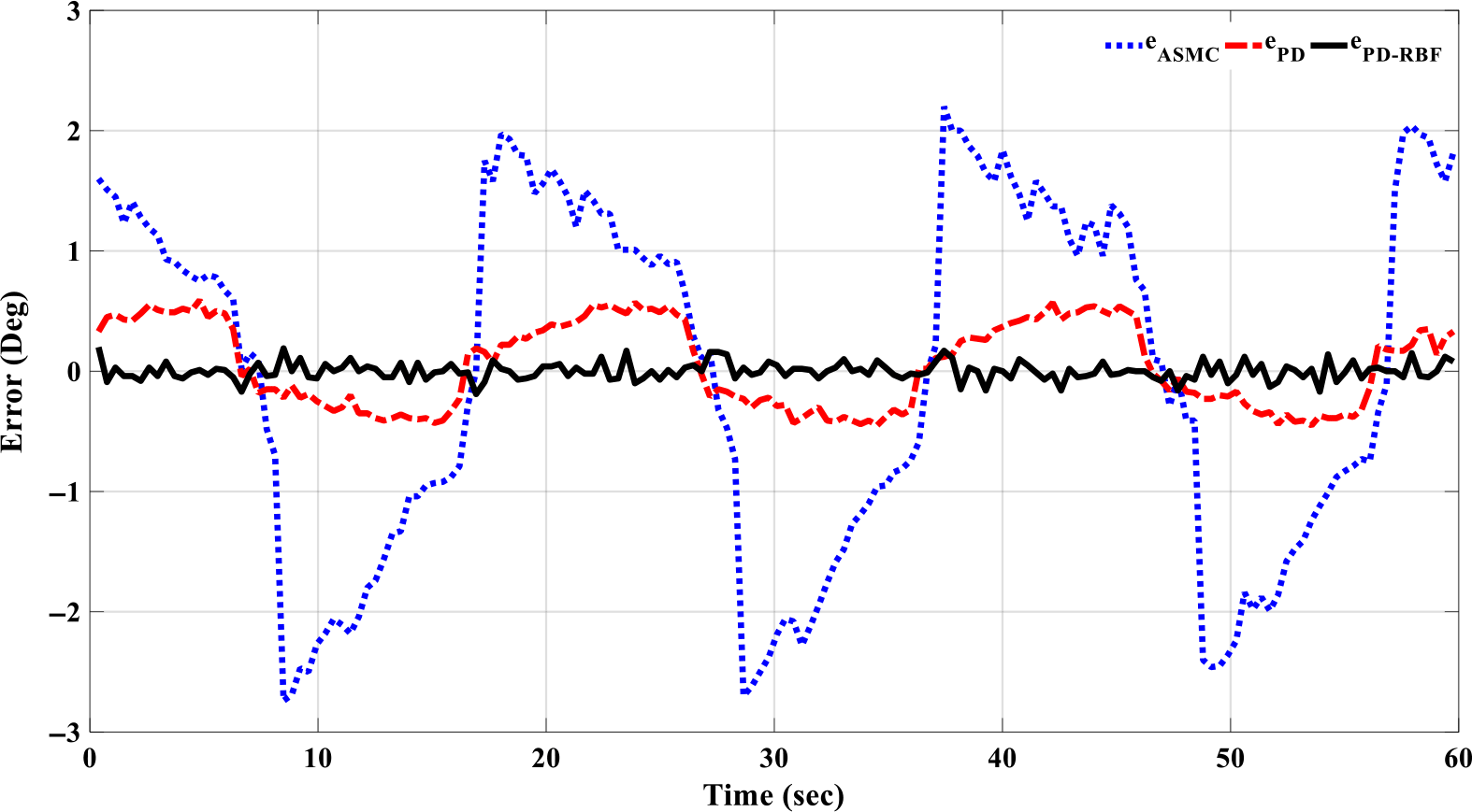
Tracking error in the passive no-load mode.

5.1. Passive mode
In this mode, the admittance control loop is disabled and the interaction torques between the KRRS and the leg are not considered. The robot follows the predefined trajectory without any changes. Figure 11 represents the predefined trajectory. First, the robot is tested, for each controller, without any load (the leg is not connected to the robot). Figure 12 shows the tracking error for the controllers in the passive no-load mode.
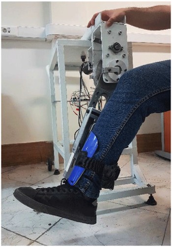
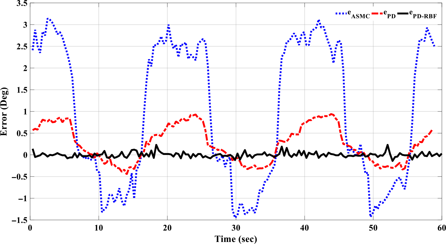
Then, the patient’s leg is connected, and the KRRS moves it along the predefined trajectory. Figure 13 shows a leg connected to the robot. Figure 14 represents the tracking error for the controllers in the passive with-load mode.
The robot with a connected leg.

Tracking error in the passive with-load mode.

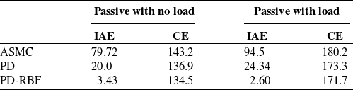
Performance indices, IAE and CE, results of each controller in this mode are reported in Table 6.
IAE and CE of the controllers in the passive mode.

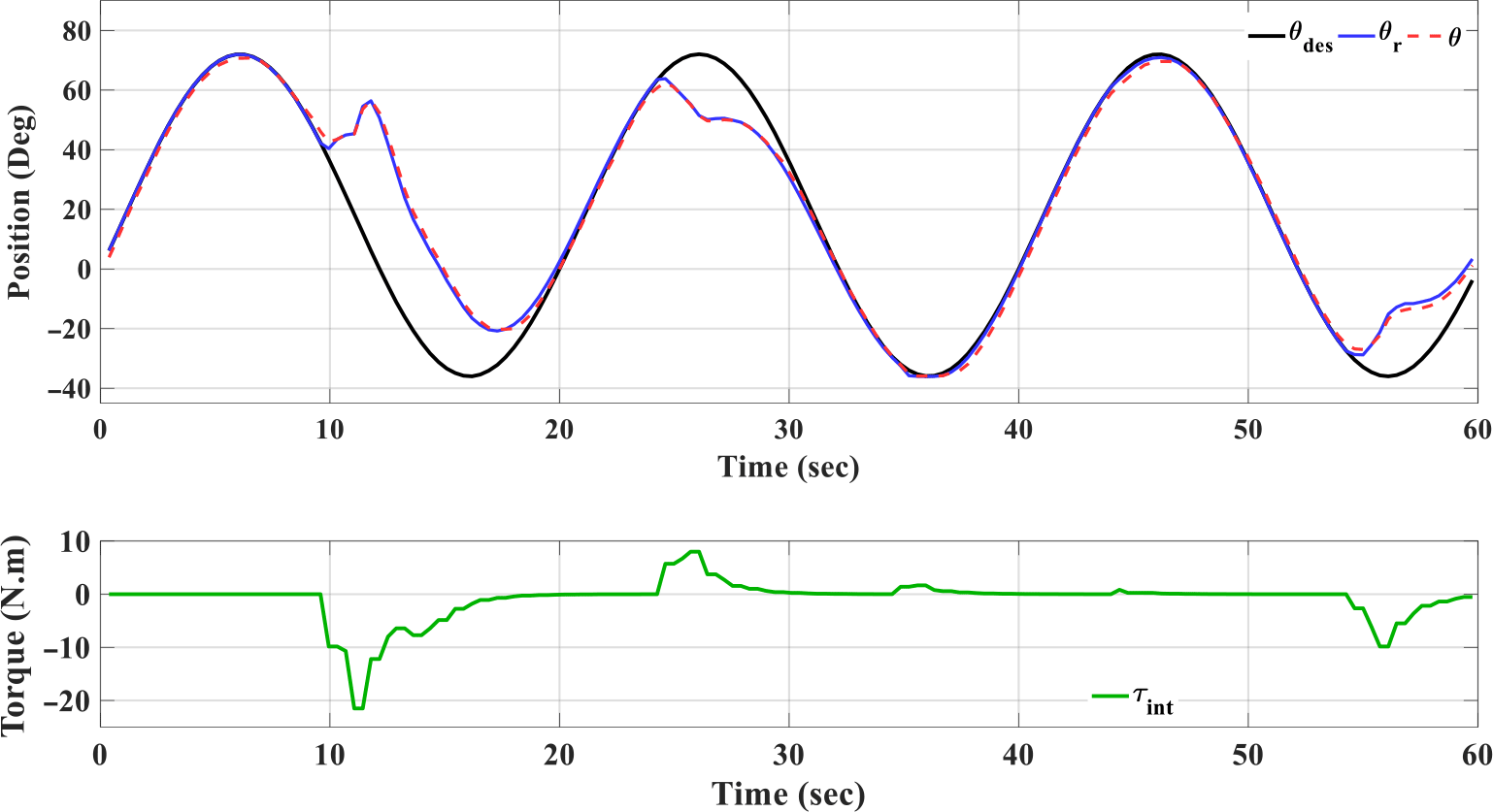
Trajectory changes in the presence of the interaction torque
 $\tau _{int}$
and tracking performance of ASMC controller.

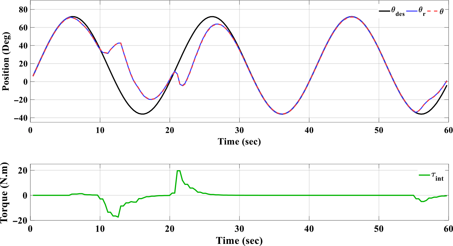
Trajectory changes in the presence of the interaction torque
 $\tau _{int}$
and tracking performance of PD controller.

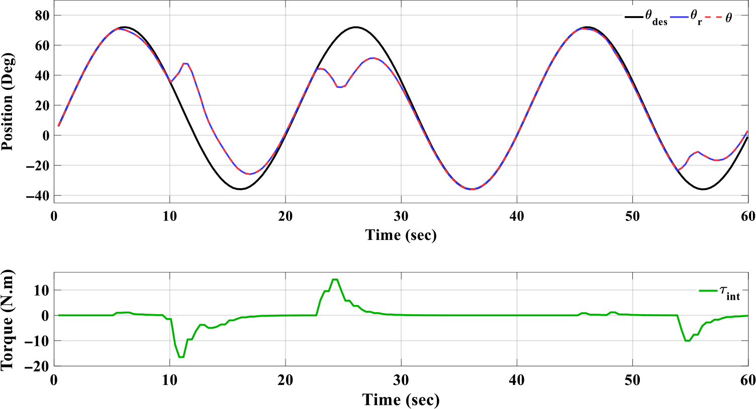
Trajectory changes in the presence of the interaction torque
 $\tau _{int}$
and tracking performance of PD-RBF controller.

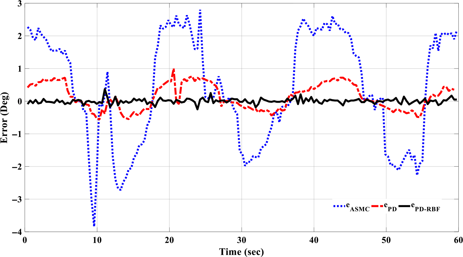
Tracking error of the ASMC, PD, and PD-RBF controllers.

5.2. Active mode
The admittance control loop is enabled in this mode, and the exerted interaction forces are measured by load cells and filtered to consider only forces of the sudden undesirable movements. Then these forces are fed back into the admittance equation, where the predefined trajectory is modified accordingly to reduce the effects of these interaction forces and ensure safe and smooth movements. Figures 15, 16, and 17 show the tracking performance of the ASMC, PD, and PD-RBF, respectively. These figures also represent how the trajectory is modified when interaction torque is applied. The tracking error of these controllers is illustrated in Fig. 18.
The CE of the robot in the active mode is subject to the interaction torques. Thus, to have a reasonable comparison between the controllers in their CE, the applied interaction torques on each of them should be similar. Since such a condition cannot be realized in practical experiment, a new ratio between the control output and the applied interaction torque is defined as follows:
 \begin{equation}\eta =\frac{\int \left| \tau \right| dt}{\int \left| \tau _{int}\right| dt}\end{equation}
 $\eta$
ratio represents the CE with respect to the interaction torques exerted by the patient.
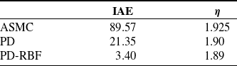
Table 7 demonstrates the IAE and the ratio
 $\eta$
for each controller in the active mode.
6. Results and discussion
In this section, the obtained results from experimental tests are analyzed, discussed, and compared. Graphical results indicate that all three controllers showed robustness in their performance, where there is no significant change in the performance for each controller in the three testing modes (passive no-load, passive with-load, and active with-load). Figures 15, 16, and 17 show that the modification in the trajectory path due to the applied interaction torques is smooth enough, with no sharp or tough changes, to provide safe movement and prohibit any injuries.
The IAE and
 $\eta$
of the controllers in the active mode.

Figures 12, 14, and 18 show the tracking error of the three controllers in the passive no-load, passive with-load, and active modes, respectively. The performance of the ASMC is highly dependent on the dynamic model, which is difficult to be computed accurately and dramatically varies according to the patient’s limb specifications. ASMC had a steady-state error ranging approximately between (−3°, 3°) in the passive mode and (−4°, 3°) in the active one. The PD performed better than the ASMC since it is a model-free control with a steady-state error less than 1° in the all modes. However, it suffers to compensate the high nonlinearity in the system. In the PD-RBF algorithm, the PD achieves the tracking task of the system, while the RBF is fed forward to compensate for the high nonlinearity terms. Thus, the controller is independent of the dynamic model of the system and able to compensate for the system’s high nonlinearity. The RBF-PD has a tracking precision higher than both PD and ASMC with a steady-state error not exceeding a peak of 0.2°. According to Tables 6 and 7, the performance indices indicate that the proposed PD-RBF has the best performance compared to the others. These outcomes prove the superiority of the PD-RBF approach over the conventional PD and ASMC.
In ref. [Reference Naghavi and Mahjoob5], a similar work is introduced. A PID controller is used in controlling 1-DOF mechanism for knee rehabilitation, and the results of that research show an error more than 2° in the passive and the active modes. In comparing the results of ref. [Reference Naghavi and Mahjoob5] with the proposed admittance PD-RBF algorithm, the admittance PD-RBF shows more accurate performance.
7. Conclusion
In this paper, a KRRS is developed. An admittance control is introduced to reduce the effects of the excessive forces between the patient’s leg and the robot. For trajectory tracking control, a PD-RBF approach is introduced, and its stability is analyzed. The performance of this developed approach, in the current paper, is compared with two linear and nonlinear control approaches. One of them is ASMC, which represents a nonlinear model-based control method, and the other one is conventional proportional-derivative control, which represents the model-free linear control technique. The ASMC is dependent on the dynamic model of the robot. In practice, the dynamic model is difficult to obtain correctly. Furthermore, the chattering phenomenon is reduced at the expense of performance accuracy. Thus, the ASMC has a high steady-state error compared with the other controllers. PD is a model-free controller, easy to be tuned compared to ASMC, has a simple structure, and does not need complicated calculation that makes it faster to force the error to converge to zero. PD has a small steady-state error due to the complex nonlinearity terms of the system. In the proposed PD-RBF, the RBF acts as a compensator for the complex nonlinearity of the system, which improves the performance of the PD controller significantly. The controller parameters are tuned experimentally for the best performance based on the considered metrics. Future works can include an improvement of the controller for online tuning of the parameters; introduce the admittance with variable parameters to possibly achieve smoother modification of the trajectory; and extend the robotic system to train the ankle joint in addition to the knee.
Funding
The authors have not received support from any organization for the submitted work.
Conflicts of interest
The authors declare that they have no conflict of interest.
Code or data availability
Data and material available on request from the authors.
Authors’ contributions
All authors contributed to all parts of the research. Design and analysis of the model were performed mainly by Bahram Tarvidizadeh and Alireza Hadi. Design and analysis of the control system were held mainly by Khalil Alipour and Karam Almaghout. All authors participated in the experiments. The first draft of the manuscript was written by Karam Almaghout, and all authors commented on the previous versions of the manuscript. All authors read and approved the final manuscript.
Ethics approval
This study was held without involving any patient and without using any patient’s data. The experiments were held in the lab by the authors themselves to evaluate the efficiency of the design and the control of the system. Thus, ethics approval was not required for this study.
Consent to participate
The authors were the only participants in this study. They were all well aware of the nature of the research, and their participation in the experiments was to benefit the system evaluation.
Consent for publication
The authors affirm that the images in Figures 1(b) and 13 belong to one of the authors who consents to publish to the benefit of the research.