1 Introduction
It is well known that a jet spreading, either radially or in two dimensions, over a plate surface may be described by a similarity solution of the laminar boundary layer equations when the Reynolds number is sufficiently high (Glauert Reference Glauert1956). If the temperature of the horizontal plate is different from the ambient temperature, and also from the temperature of the emerging jet, buoyancy forces may be relevant, coupling the temperature and the velocity fields of the flow over the plate. Mixed-convection problems over a horizontal plate have been widely studied in the past due to their engineering, as well as theoretical, interest. For instance, for a constant external velocity above the plate, the problem has a similarity solution for specific power-law temperature distributions on the horizontal plate (Sparrow, Eichhorn & Gregg Reference Sparrow, Eichhorn and Gregg1959; Gill & del Casal Reference Gill and del Casal1962; Leal Reference Leal1973; Schneider Reference Schneider1979; Afzal & Hussain Reference Afzal and Hussain1984; Denier, Duck & Li Reference Denier, Duck and Li2005; Deswita et al. Reference Deswita, Nazar, Ishak, Ahmad and Pop2010), but not for the case of a constant temperature plate. The solutions for the cases of an insulated and of a cooled horizontal plate present some interesting features, such as singularity and non-uniqueness (Schneider & Wasel Reference Schneider and Wasel1985; Daniels Reference Daniels1992; Daniels & Gargaro Reference Daniels and Gargaro1993; Steinrück Reference Steinrück1994, Reference Steinrück1995; Higuera Reference Higuera1997; Denier et al. Reference Denier, Duck and Li2005), which are not found for the case of the flow over a heated horizontal plate at constant temperature (Fernandez-Feria, del Pino & Fernandez-Gutierrez Reference Fernandez-Feria, del Pino and Fernandez-Gutierrez2014). In particular, for an insulated plate, a similarity solution exists provided that the local Froude number, measuring the importance of inertia relative to buoyancy, is above a threshold value. Below this value the boundary layer approximation fails either by the onset of reverse flow or more generally by the occurrence of a terminal singularity associated with a sudden rise in skin friction (Daniels Reference Daniels1992; Daniels & Gargaro Reference Daniels and Gargaro1993). On the other hand, flow separation from the wall occurs for sufficiently small Froude numbers in the case of a two-dimensional jet over a cooled plate (Higuera Reference Higuera1997), or in the case of a radial flow above a heated plate when the Grashof number based on the radius of the issued external velocity is sufficiently small (Fernandez-Feria et al. Reference Fernandez-Feria, del Pino and Fernandez-Gutierrez2014).
We consider here the case of a vanishing external velocity far above the plate, i.e. the case of a wall jet spreading radially or in two dimensions, but taking into account the coupling of the temperature and velocity fields by buoyancy when the plate temperature remains constant and higher than the ambient temperature. We show that this problem, when governed by a boundary layer approximation for a sufficiently high Reynolds number, has a far-field similarity solution valid for both the radial flow and the two-dimensional flow. The wall jet structure described by this similarity solution is radically different from Glauert’s (Reference Glauert1956) similarity solution without buoyancy forces, and qualitatively different (although mathematically equivalent in the two-dimensional case) from Stewartson’s (Reference Stewartson1958) similarity solution for the purely free convection problem over a horizontal surface. To the best of our knowledge, the solution has not been described in the literature.
The similarity solution is obtained in § 3, where it is demonstrated that it exists only for a heated plate for any value of the Froude number (whose inverse is named
 ${\it\Lambda}$
), but not for a cooled plate. To check numerically the existence of the similarity solution, and to define the different non-dimensional parameters governing the problem, we present first in § 2 a particular problem where a uniform jet with constant velocity and temperature emerges from a slot of height
 ${\it\delta}$
and radius
 $r_{0}$
(in the radially spreading case). Both the radial (or axisymmetric) and the two-dimensional problems are formulated together, just differing in the value of an index, to facilitate the comparison of their results. The wall jet in absence of buoyancy forces is also included as the case
 ${\it\Lambda}=0$
. To start the numerical integration of the resulting parabolic, integro-differential equations, we use an approximate similarity solution valid near the jet exit that contains the first-order effect due to the buoyancy forces on the jet (described in appendix A). This solution is also used to validate the numerical method, which is described in § 4. The main numerical results are described and discussed also in § 4, while some conclusions are drawn in § 5.
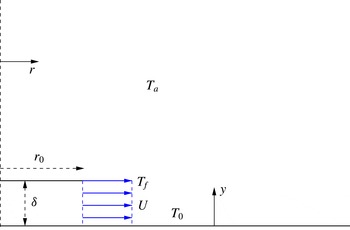
Schematic of the problem (with dimensional variables and parameters).

2 Formulation of the problem
We consider in this section a planar jet flow spreading over a horizontal plate, which is set at a constant temperature
 $T_{0}$
higher than the ambient temperature
 $T_{a}$
, of a fluid emerging radially with uniform velocity
 $U$
and temperature
 $T_{f}\leqslant T_{0}$
from a circular slot of radius
 $r_{0}$
and height
 ${\it\delta}$
(see figure 1; in the two-dimensional case, the uniform jet emerges from
 $r=0$
). Assuming that the Reynolds number based on
 $U$
and
 ${\it\delta}$
is sufficiently large,
 $$\begin{eqnarray}Re=\frac{U{\it\delta}}{{\it\nu}}\gg 1,\end{eqnarray}$$
where
 ${\it\nu}$
is the kinematic viscosity of the fluid at the reference temperature
 $T_{a}$
, a boundary layer approximation can be used. Assuming also axisymmetry of the flow, scaling the horizontal coordinate
 $r$
with
 $L\equiv {\it\delta}^{2}U/{\it\nu}$
, the vertical coordinate
 $y$
with
 ${\it\delta}$
, the horizontal velocity component
 $u$
with
 $U$
, the vertical velocity component
 $v$
with
 $U\,Re^{-1}=U{\it\delta}/L$
, and using the Boussinesq approximation to model the buoyancy effects induced by the temperature difference, with non-dimensional temperature defined as
 ${\it\theta}=(T-T_{a})/(T_{0}-T_{a})$
, the governing non-dimensional (continuity, momentum and energy) equations can be written as (Fernandez-Feria et al.
Reference Fernandez-Feria, del Pino and Fernandez-Gutierrez2014)
 $$\begin{eqnarray}\frac{1}{r^{\,j}}\frac{\partial }{\partial r}(r^{\,j}u)+\frac{\partial v}{\partial y}=0,\end{eqnarray}$$
 $$\begin{eqnarray}u\frac{\partial u}{\partial r}+v\frac{\partial u}{\partial y}-\frac{\partial ^{2}u}{\partial y^{2}}={\it\Lambda}\frac{\partial }{\partial r}\int _{y}^{\infty }{\it\theta}\,\text{d}y,\end{eqnarray}$$
 $$\begin{eqnarray}u\frac{\partial {\it\theta}}{\partial r}+v\frac{\partial {\it\theta}}{\partial y}=\frac{1}{Pr}\frac{\partial ^{2}{\it\theta}}{\partial y^{2}},\end{eqnarray}$$
where
 $$\begin{eqnarray}Pr=\frac{{\it\nu}}{{\it\alpha}}\quad \text{and}\quad {\it\Lambda}=\frac{{\it\beta}g{\it\delta}(T_{0}-T_{a})}{U^{2}}=\frac{Gr}{Re^{2}}\end{eqnarray}$$
are the Prandtl number and a non-dimensional parameter related to the Grashof (
 $Gr$
) and Reynolds numbers, respectively, with
 ${\it\alpha}$
and
 ${\it\beta}$
the thermal diffusivity and thermal expansivity of the fluid at the reference temperature
 $T_{a}$
, respectively, and
 $g$
the acceleration due to gravity (
 ${\it\beta}=1/T_{a}$
for an ideal gas). An index
 $j$
has been used in (2.2) to include in the same formulation the axisymmetric radial flow, corresponding to
 $j=1$
, and the two-dimensional (2D) flow, corresponding to
 $j=0$
, so that one may easily compare the results from both configurations. Note that the last term in the horizontal momentum equation (2.3) represents the pressure gradient due to buoyancy forces induced by the temperature difference when the Boussinesq approximation is used. It is written here as an integro-differential term once the horizontal pressure gradient is transformed by using the vertical momentum equation,
 $$\begin{eqnarray}0=-\frac{\partial p}{\partial y}+{\it\Lambda}{\it\theta},\end{eqnarray}$$
where the relative pressure
 $p$
is scaled with
 ${\it\rho}_{a}U^{2}$
, with
 ${\it\rho}_{a}$
the fluid density at ambient temperature, after eliminating the pressure by cross-differentiation of the horizontal and the vertical momentum equations, and integrating the resulting equation across the boundary layer:
 $$\begin{eqnarray}u\frac{\partial u}{\partial r}+v\frac{\partial u}{\partial y}=\frac{\partial ^{2}u}{\partial y^{2}}-\left.\frac{\partial ^{2}u}{\partial y^{2}}\right|_{y=0}-{\it\Lambda}\frac{\partial }{\partial r}\int _{0}^{y}{\it\theta}\,\text{d}y,\end{eqnarray}$$
 $$\begin{eqnarray}\left.\frac{\partial ^{2}u}{\partial y^{2}}\right|_{y=0}=\left.\frac{\partial p}{\partial r}\right|_{y=0}=-{\it\Lambda}\frac{\partial }{\partial r}\int _{0}^{\infty }{\it\theta}\,\text{d}y.\end{eqnarray}$$
This coupling of the temperature and velocity fields by buoyancy is characterized by the non-dimensional parameter
 ${\it\Lambda}$
, which is akin to the inverse of a Froude number (Daniels Reference Daniels1992; Higuera Reference Higuera1997).
The boundary conditions can be written as
 $$\begin{eqnarray}u=v=0,\quad {\it\theta}=1\quad \text{at }y=0,\end{eqnarray}$$
 $$\begin{eqnarray}u={\it\theta}=0\quad \text{as }y\rightarrow \infty ,\end{eqnarray}$$
 $$\begin{eqnarray}u=\left\{\begin{array}{@{}lr@{}}1, & y\leqslant 1\\ 0, & y>1,\end{array}\right.\quad {\it\theta}=\left\{\begin{array}{@{}lr@{}}{\it\theta}_{f}, & y\leqslant 1\\ 0, & y>1\end{array}\right.\text{ at }r=j\,R_{0},\end{eqnarray}$$
where
 $$\begin{eqnarray}{\it\theta}_{f}=\frac{T_{f}-T_{a}}{T_{0}-T_{a}},\quad R_{0}=\frac{r_{0}}{L}=\frac{1}{Re}\frac{r_{0}}{{\it\delta}}.\end{eqnarray}$$
The problem is thus governed by four non-dimensional parameters:
 $Pr$
,
 ${\it\Lambda}$
,
 ${\it\theta}_{f}$
and
 $R_{0}$
. In the 2D flow (
 $j=0$
), the last one disappears.
 ${\it\theta}_{f}$
also vanishes in the particular case in which the fluid enters at the ambient temperature (
 $T_{f}=T_{a}$
). Finally,
 ${\it\Lambda}=0$
corresponds to the case without thermal or natural convection effects, i.e. the classical wall jet considered by Glauert (Reference Glauert1956).
3 Similarity solution far from the jet exit
To integrate numerically (2.2)–(2.11) one may start from a self-similar solution valid near the jet exit, i.e. for
 ${\it\zeta}\equiv r-j\,R_{0}\ll 1$
, given in appendix A. This will be done in § 4 for several significant values of the non-dimensional parameters. But, before that, it is of interest to search for a more general similarity solution of the problem valid in the opposite limit far from the jet exit,
 $r\gg \max (1,jR_{0})$
. Then we shall compare its structure, if such solution exists, with the numerical solution.
Defining the non-dimensional stream function
 ${\it\psi}$
as
 $$\begin{eqnarray}u=\frac{1}{r^{\,j}}\frac{\partial {\it\psi}}{\partial y},\quad v=-\frac{1}{r^{\,j}}\frac{\partial {\it\psi}}{\partial r},\end{eqnarray}$$
in terms of which the continuity equation (2.2) is identically satisfied, we look for solutions of (2.3)–(2.4) in the form
 $$\begin{eqnarray}{\it\psi}=Ar^{a}f({\it\tau}),\quad {\it\theta}=Cr^{c}g({\it\tau}),\quad {\it\tau}=B\frac{y}{r^{b}},\end{eqnarray}$$
where
 $a$
,
 $b$
and
 $c$
are constants, compatible with the boundary conditions (2.9)–(2.10), but disregarding the ‘initial’ condition (2.11a,b
). Constants
 $A$
,
 $B$
and
 $C$
are selected to eliminate from the resulting similarity problem as many parameters as possible. Clearly,
 $$\begin{eqnarray}c=0\quad \text{and}\quad C=1\end{eqnarray}$$
to satisfy the temperature boundary condition at the wall
 $g\,({\it\tau}=0)=1$
. From (3.1) and (3.2),
 $$\begin{eqnarray}u=ABr^{a-b-j}f^{\prime },\quad v=-Ar^{a-1-j}(af-b{\it\tau}f^{\prime }),\end{eqnarray}$$
where the primes denote differentiation with respect to
 ${\it\tau}$
. Substituting into (2.3)–(2.10) one gets
 $$\begin{eqnarray}\frac{1}{5}\,f^{\prime 2}-\left(j+\frac{3}{5}\right)ff^{\prime \prime }-f^{\prime \prime \prime }={\it\tau}g+\int _{{\it\tau}}^{\infty }g\,\text{d}{\it\tau},\end{eqnarray}$$
 $$\begin{eqnarray}g^{\prime \prime }+Pr(j+{\textstyle \frac{3}{5}})fg^{\prime }=0,\end{eqnarray}$$
 $$\begin{eqnarray}f(0)=f^{\prime }(0)=f^{\prime }(\infty )=g(\infty )=0,\quad g(0)=1,\end{eqnarray}$$
with
 $$\begin{eqnarray}a=j+\frac{3}{5},\quad b=\frac{2}{5},\quad A=B=\left(\frac{2{\it\Lambda}}{5}\right)^{1/5}.\end{eqnarray}$$
This selection of
 $A$
and
 $B$
eliminates the non-dimensional parameter
 ${\it\Lambda}$
from the problem (3.5)–(3.7), which thus only depends on
 $Pr$
and
 $j$
, so that the similarity solutions contains explicitly its dependence on
 ${\it\Lambda}$
(see below). Curiously, the similarity variable
 ${\it\tau}$
is the same in both the 2D and the axisymmetric cases (
 $j=0$
and
 $1$
),
 $$\begin{eqnarray}{\it\tau}=\left(\frac{2{\it\Lambda}}{5}\right)^{1/5}\frac{y}{r^{2/5}},\end{eqnarray}$$
and so is the horizontal or radial dependence of
 $u$
,
 $$\begin{eqnarray}u=\left(\frac{2{\it\Lambda}}{5}\right)^{2/5}r^{1/5}f^{\prime }({\it\tau}).\end{eqnarray}$$
This contrasts Glauert’s (Reference Glauert1956) similarity solution for the case without buoyancy forces, whose horizontal variation depends on
 $j$
: in our notation,
 $u\sim r^{-(j+1/2)}f_{G}^{\prime }({\it\tau}_{G})$
, where
 ${\it\tau}_{G}\sim y/r^{(j+3/2)/2}$
(see § 4.2 below for more details) and
 $f_{G}$
satisfies equation (4.1) in Glauert (Reference Glauert1956),
 $$\begin{eqnarray}2f_{G}^{\prime 2}+f_{G}f_{G}^{\prime }+f_{G}^{\prime \prime \prime }=0,\quad f_{G}(0)=f_{G}^{\prime }(0)=f_{G}^{\prime }(\infty )=0.\end{eqnarray}$$
In the present similarity solution, only the vertical velocity
 $v$
depends explicitly on the radial divergence of the flow,
 $$\begin{eqnarray}v=-\left(\frac{2{\it\Lambda}}{5}\right)^{1/5}r^{-2/5}\left[\left(j+\frac{3}{5}\right)f-\frac{2}{5}{\it\tau}f^{\prime }\right],\end{eqnarray}$$
although both functions
 $f$
and
 $g$
depend on
 $j$
through (3.5)–(3.6), in terms of which the non-dimensional stream function and temperature can be written as
 $$\begin{eqnarray}{\it\psi}=\left(\frac{2{\it\Lambda}}{5}\right)^{1/5}r^{j+3/5}f({\it\tau}),\quad {\it\theta}=g({\it\tau}).\end{eqnarray}$$
Note that, according to (3.10), the maximum of
 $u$
grows slowly with
 $r$
, while in Glauert’s solution the maximum of
 $u$
decays with
 $r$
for both
 $j=0$
and
 $j=1$
(see also § 4). The temperature field corresponding to Glauert’s solution behaves, for the case of a 2D flow (
 $j=0$
), as
 ${\it\theta}\sim r^{-1/4}g_{G}({\it\tau}_{G})$
(Daniels & Gargaro Reference Daniels and Gargaro1992), whose downstream evolution is also qualitatively very different from that given by (3.13).
It is also worth noticing here that, for
 $j=0$
, the problem (3.5)–(3.7) is mathematically quite similar to the purely free convection problem analysed by Stewartson (Reference Stewartson1958) (see also Schlichting & Gersten Reference Schlichting and Gersten2000, § 10.6). However, the similarity variables (3.9)–(3.10) and (3.13) are qualitatively different from those of Stewartson because here we have a mixed-convection problem governed by
 ${\it\Lambda}$
, the inverse of a Froude number, that contains a characteristic horizontal speed
 $U$
. In addition, only the two-dimensional (
 $j=0$
) flow was considered, while
 $r$
stands here for the streamwise coordinate in both the 2D flow and the radially spreading flow.
The problem (3.5)–(3.7) has a solution for any value of
 $Pr$
, for
 $j=0$
and
 $j=1$
, which can be easily obtained numerically by standard numerical methods. This means that, according to the above similarity variables, a similarity solution far from the jet exit exists for any
 ${\it\Lambda}>0$
, but no solution exists for
 ${\it\Lambda}\leqslant 0$
. In fact, for
 ${\it\Lambda}=0$
, the structure of the flow, which corresponds to Glauert’s similarity solution, is quite different, as indicated above, while for
 ${\it\Lambda}<0$
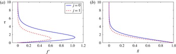
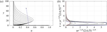
, i.e. for a cooled plate, no similarity solution exists at all, in agreement with some previous works referred to in § 1. Figure 2 shows the scaled vertical profiles of the radial velocity,
 $f^{\prime }({\it\tau})=r^{-1/5}(2{\it\Lambda}/5)^{-2/5}\,u$
, and the temperature,
 $g\,({\it\tau})={\it\theta}$
, for
 $Pr=0.7$
(e.g. air) in the 2D flow and in the axisymmetric case. The structure of the solutions for other values of
 $Pr$
is quite similar, with different slopes at the wall
 $y=0$
. In § 4 we shall check that the numerical solution of (2.2)–(2.11a,b
) tends to this similarity solution far from the exit provided that
 ${\it\Lambda}>0$
, for any value of
 $j$
,
 $Pr$
and
 ${\it\theta}_{f}$
. For
 ${\it\Lambda}=0$
, we shall show that the numerical solution tends to Glauert’s similarity solution, which is radically different, as already commented on, while for
 ${\it\Lambda}<0$
no similarity solution will be reached at all.


Of particular interest are the local skin friction coefficient at the wall and the local Nusselt number (or non-dimensional heat transfer at the wall), whose radial variations and their dependence on
 ${\it\Lambda}$
are given explicitly from the similarity variables:
 $$\begin{eqnarray}c_{f}\equiv \left.\frac{\partial u}{\partial y}\right|_{y=0}=f^{\prime \prime }(0)\left(\frac{2{\it\Lambda}}{5}\right)^{3/5}r^{-1/5},\end{eqnarray}$$
 $$\begin{eqnarray}Nu\equiv -\!\left.\frac{\partial {\it\theta}}{\partial y}\right|_{y=0}=-g^{\prime }(0)\left(\frac{2{\it\Lambda}}{5}\right)^{1/5}r^{-2/5}.\end{eqnarray}$$
Also of physical interest is the radial or horizontal pressure gradient, which depends on
 $y$
due to the buoyancy forces. At the wall, the non-dimensional radial pressure gradient can be written as
 $$\begin{eqnarray}\left.\frac{\partial p}{\partial r}\right|_{y=0}=-{\it\Lambda}\frac{\partial }{\partial r}\int _{0}^{\infty }{\it\theta}\,\text{d}y=-G(0)\left(\frac{2{\it\Lambda}}{5}\right)^{4/5}r^{-3/5},\end{eqnarray}$$
where
 $$\begin{eqnarray}G({\it\tau})\equiv \int _{{\it\tau}}^{\infty }g({\it\tau})\,\text{d}{\it\tau}\geqslant 0.\end{eqnarray}$$
Note that the similarity solution is valid only far from the jet exit, so that the singularities as
 $r\rightarrow 0$
in (3.14)–(3.16) are not physically relevant. It is clear that the horizontal pressure gradient at the wall is always negative, i.e. if the present self-similar solution is reached, no adverse pressure gradient is generated in the boundary layer flow, vanishing as
 $r\rightarrow \infty$
. The absolute value of the radial pressure gradient at any other height
 $y$
is always smaller than that at the wall, since the maximum of
 $G({\it\tau})$
is reached at
 ${\it\tau}=0$
.
The dependencies on
 $j$
and on
 $Pr$
of
 $f^{\prime \prime }(0)$
,
 $g^{\prime }(0)$
and
 $G(0)$
, and, therefore, the variation with
 $j$
and
 $Pr$
of
 $c_{f}$
,
 $Nu$
and the pressure gradient, have to be obtained numerically. Actually, the variation with
 $Pr$
obtained numerically can be fitted to simple power laws very accurately, valid for any
 $Pr$
in the case of
 $c_{f}$
, and for
 $Pr\lesssim 1$
or
 $Pr\gtrsim 3$
in the case of
 $Nu$
and the pressure gradient:
 $$\begin{eqnarray}f^{\prime \prime }(0)\simeq \left\{\begin{array}{@{}lr@{}}1.48\,Pr^{-0.38}, & j=0,\\ 1.04\,Pr^{-0.38}, & j=1,\end{array}\right.\quad \text{for any }Pr,\end{eqnarray}$$
 $$\begin{eqnarray}g^{\prime }(0)\simeq \left\{\begin{array}{@{}lr@{}}-0.47\,Pr^{1/3}, & j=0,\\ -0.62\,Pr^{1/3}, & j=1,\end{array}\right.\quad \text{for }Pr\lesssim 1,\end{eqnarray}$$
 $$\begin{eqnarray}g^{\prime }(0)\simeq \left\{\begin{array}{@{}lr@{}}-0.49\,Pr^{0.22}, & j=0,\\ -0.60\,Pr^{0.22}, & j=1,\end{array}\right.\quad \text{for }Pr\gtrsim 3,\end{eqnarray}$$
 $$\begin{eqnarray}G(0)\simeq \left\{\begin{array}{@{}lr@{}}1.25\,Pr^{-0.36}, & j=0,\\ 1.00\,Pr^{-0.36}, & j=1,\end{array}\right.\quad \text{for }Pr\lesssim 1,\end{eqnarray}$$
 $$\begin{eqnarray}G(0)\simeq \left\{\begin{array}{@{}lr@{}}1.23\,Pr^{-0.23}, & j=0,\\ 1.00\,Pr^{-0.23}, & j=1,\end{array}\right.\quad \text{for }Pr\gtrsim 3.\end{eqnarray}$$
Some of these approximations can be refined using the formal integration of (3.6) that provides a general expression for
 $g$
in terms of
 $f$
:
 $$\begin{eqnarray}g=1+g^{\prime }(0)\int _{0}^{{\it\tau}}\exp \left[-\left(j+\frac{3}{5}\right)Pr\int _{0}^{{\it\tau}}f\,\text{d}{\it\tau}\right]\text{d}{\it\tau},\end{eqnarray}$$
where the boundary condition
 $g\,(0)=1$
has been used. On using the other boundary condition for
 $g$
,
 $$\begin{eqnarray}g^{\prime }(0)=-\left\{\int _{0}^{\infty }\exp \left[-\left(j+\frac{3}{5}\right)Pr\int _{0}^{{\it\tau}}f\,\text{d}{\it\tau}\right]\,\text{d}{\it\tau}\right\}^{-1}.\end{eqnarray}$$
These expressions can be used to obtain the dependencies of
 $g^{\prime }(0)$
and
 $G(0)$
with
 $Pr$
in the limits
 $Pr\ll 1$
and
 $Pr\gg 1$
. But, since they depend on
 $f({\it\tau})$
, which has to be obtained numerically, the procedure has no real advantage from the purely numerical one used above.
It is also of practical interest to write (3.14) and (3.15) in terms of the Grashof number (
 $Gr={\it\beta}g{\it\delta}^{3}(T_{0}-T_{a})/{\it\nu}^{2}$
) explicitly:
 $$\begin{eqnarray}c_{f}=f^{\prime \prime }(0)\left(\frac{2}{5}\right)^{3/5}\frac{Gr^{3/5}}{Re}\bar{r}^{-1/5},\end{eqnarray}$$
 $$\begin{eqnarray}Nu=-g^{\prime }(0)\left(\frac{2}{5}\right)^{1/5}Gr^{1/5}\bar{r}^{-2/5},\end{eqnarray}$$
where
 $\bar{r}$
is the non-dimensional radial distance scaled with
 ${\it\delta}$
instead of
 $L$
(i.e.
 $\bar{r}=Re\,r$
). Thus,
 $Nu\propto Pr^{1/3}Gr^{1/5}\bar{r}^{-2/5}$
for
 $Pr\lesssim 1$
and
 $Nu\propto Pr^{0.22}Gr^{1/5}\bar{r}^{-2/5}$
for
 $Pr\gtrsim 3$
, and it does not depend on
 $Re$
.
4 Numerical results and discussion
4.1 Numerical method and validation
To integrate numerically the problem (2.2)–(2.11a,b
) we use a pseudospectral-based method of lines, as described in Fernandez-Feria & Ortega-Casanova (Reference Fernandez-Feria and Ortega-Casanova2014). The vertical velocity
 $v$
is written in terms of
 $u$
from (2.2) and substituted into (2.3)–(2.4). The resulting integro-differential equations for
 $u$
and
 ${\it\theta}$
are discretized in the vertical direction using a Chebyshev pseudospectral collocation method. Then, the set of ordinary differential equations on the collocation points is integrated in the radial direction using an accurate method of lines, starting from the approximate similarity solution described in appendix A at a given
 $r_{in}={\it\zeta}_{in}+jR_{0}$
, with
 ${\it\zeta}_{in}\ll 1$
and
 ${\it\zeta}_{in}\ll R_{0}$
(if
 $j=1$
).
To discretize the equations along the vertical direction we concentrate the collocation nodes near the plate
 $y=0$
and near
 $y=1$
, where the velocity gradients are very large close to the jet exit. To that end we use the following transformations to map the Chebyshev collocation points
 $s_{i}=\cos (\text{i}{\rm\pi}/N)$
,
 $i=0,1,\ldots ,N$
, defined in the interval [
 $-1,1$
], into the computational nodes
 $y_{i}$
in the domain [
 $0,\infty$
):
 $$\begin{eqnarray}t_{i}=\frac{a(1+s_{i})}{2a/t_{M}+1-s_{i}},\quad y_{i}=a_{0}\frac{1-\text{e}^{-mt_{i}}}{b_{0}+\text{e}^{-mt_{i}}}\,+c_{0}t_{i}\text{e}^{t_{i}/t_{M}-1},\quad i=0,1,\ldots ,N.\end{eqnarray}$$
The first transformation maps the interval [
 $-1,1$
] onto [
 $0,t_{M}$
], where
 $t_{M}\gg 1$
is related to the point
 $y_{M}\gg 1$
(see below) at which the boundary conditions as
 $y\rightarrow \infty$
are imposed. Approximately half the nodes are in
 $0\leqslant t\leqslant a$
, thus concentrating the nodes near the plate (we choose
 $a=2$
and
 $t_{M}=1000$
in all the reported computations). The second transformation, mapping
 $0\leqslant t_{i}\leqslant t_{M}$
onto
 $0\leqslant y_{i}\leqslant y_{M}$
, concentrates the computational nodes near
 $y=1$
, maintaining their high concentration close to the plate and their sparseness far from the plate. Note that
 $y_{M}\approx c_{0}t_{M}$
if
 $a_{0}/b_{0}$
is order unity (
 $y_{M}\simeq 500$
in all the reported computations). The values of the parameters used in all the computations reported below are
 $a_{0}=0.04$
,
 $b_{0}=0.0548$
,
 $c_{0}=0.5$
,
 $m=6$
, and
 $N$
between
 $80$
and
 $200$
. Note that
 $i=N$
corresponds to the plate (
 $y_{N}=0$
) and
 $i=0$
to the point at infinity (
 $y_{0}=y_{M}$
).
In addition to the Chebyshev collocation points with the above transformations we also tried a Laguerre pseudospectral collocation method, since Laguerre collocation points are already distributed in [
 $0,\infty$
) (Boyd Reference Boyd2000). But, after using the second transformation (4.1) on Laguerre’s points to concentrate the nodes near
 $y=1$
, the method yielded poorer results. The reason was that Laguerre collocation points are not sufficiently packed near
 $y=0$
for the same
 $y_{M}$
, so that one has to use a much higher number of nodes
 $N$
than with the above transformations of Cbebyshev’s collocation points to obtain the same accuracy near the plate.
Another numerical difficulty, apart from the required node concentration at
 $y=0$
and
 $y=1$
to start the numerical integration, is the boundary condition of
 $u$
as
 $y\rightarrow \infty$
(implemented at
 $y_{M}$
). Since
 $u$
tends to zero there, the mass matrix
 $\unicode[STIX]{x1D648}$
in the method of lines (Fernandez-Feria & Ortega-Casanova Reference Fernandez-Feria and Ortega-Casanova2014) becomes very ill conditioned or close to singular, depending on
 $y_{M}$
and on the number of nodes
 $N$
. To circumvent this difficulty, we replaced that boundary condition in (2.10) by
 $u(r,y_{M})={\it\epsilon}\ll 1$
. In most reported computations we choose
 ${\it\epsilon}=4\times 10^{-3}$
.
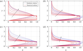
To validate the numerical integration, checking its agreement with the approximate self-similar solution for small
 ${\it\zeta}$
given in appendix A, figure 3 shows the vertical profiles of
 $u$
for the 2D case (
 $j=0$
) and for the radial case (
 $j=1$
) with
 $R_{0}=0.1$
, for
 ${\it\Lambda}=0$
and
 ${\it\Lambda}=1$
. The numerical solutions are obtained starting at
 ${\it\zeta}_{i}=3\times 10^{-4}$
from the self-similar approximation for
 ${\it\zeta}\ll 1$
using
 $N=160$
pseudospectral nodes in the vertical direction from
 $y=0$
to
 $y=y_{M}\simeq 500$
, where the boundary conditions as
 $y\rightarrow \infty$
are set, and Matlab’s ode23t code (with default error tolerance values) to advance in the horizontal direction solving the ordinary differential equations resulting from the method of lines. It is observed that the accuracy of the numerical solutions is quite satisfactory with these numerical parameters, since they practically coincide with the self-similar ones at least up to
 ${\it\zeta}=0.0048$
in all cases. Actually, the self-similar solution becomes poorer faster as
 ${\it\zeta}$
increases in the axisymmetric case due to the radial divergence of the flow, particularly for
 ${\it\Lambda}\neq 0$
, an effect that is more important as
 $R_{0}$
decreases. In the 2D case (
 $j=0$
) with
 ${\it\Lambda}=0$
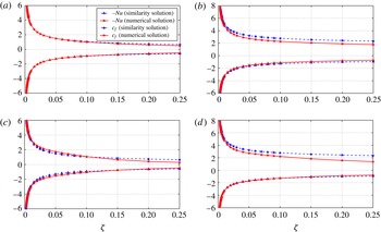
, the approximate self-similar solution with the two terms given in appendix A remains quite accurate up to
 ${\it\zeta}\sim 0.1$
, as is more clearly observed in figure 4(a), while for
 ${\it\Lambda}=1$
and
 $j=1$
with
 $R_{0}=0.1$
(figure 4
d) the self-similar solution is already quite poor for
 ${\it\zeta}\sim 0.025$
. These figures show the horizontal evolutions of the non-dimensional skin friction at the wall (
 $c_{f}$
) and heat flux at the wall (
 $-Nu$
, the minus sign is just to separate the curves in the same plot) computed both numerically and with the similarity solution valid for
 ${\it\zeta}=r-jR_{0}\ll 1$
.
Comparison of the vertical profiles of the radial velocity computed numerically with those from the similarity solution valid for
 ${\it\zeta}\ll 1$
for several values of
 ${\it\zeta}$
: 0.0003, 0.0014, 0.0028, 0.0048, 0.01, 0.025, 0.05, 0.08, 0.1, increasing in the direction of the arrow. 2D case (a,b) and axisymmetric case with
 $R_{0}=0.1$
(c,d) for
 ${\it\Lambda}=0$
(a,c) and
 ${\it\Lambda}=1$
(b,d).
 $Pr=0.7$
,
 ${\it\theta}_{f}=0$
: (a,b)
 $j=0$
, (c,d)
 $j=1$
.

Comparison of the radial variation of
 $-Nu$
and
 $c_{f}$
computed numerically with those from the similarity solution valid for
 ${\it\zeta}\ll 1$
,
 $j=0$
for the 2D case (a,b) and for the axisymmetric case (
 $j=1$
) with
 $R_{0}=0.1$
(c,d), with
 ${\it\Lambda}=0$
(a,c) and
 ${\it\Lambda}=1$
(b,d).
 $Pr=0.7$
,
 ${\it\theta}_{f}=0$
.

The vertical gradients of the fluid magnitudes (particularly of
 $u$
and
 $v$
) are very strong near
 $y=0$
and
 $y=1$
only close to the jet exit (small
 ${\it\zeta}$
). As the flow moves forward the vertical gradients around these points decay very fast, becoming more uniformly distributed along the vertical direction. Therefore, it is not necessary to keep the high node concentrations near these points. For this reason, after the initial numerical difficulties are circumvented with the above-defined transformations, we restarted the numerical integration along
 $r$
at
 ${\it\zeta}=5$
using a more uniform node distribution, with just the first transformation in (4.1) with
 $a=30$
for
 ${\it\Lambda}\neq 0$
and
 $a=50$
for
 ${\it\Lambda}=0$
. All the numerical solutions reported below are computed following this scheme: with a high concentration of nodes both near
 $y=0$
and near
 $y=1$
up to
 ${\it\zeta}=5$
, and then using a more uniform node distribution from
 ${\it\zeta}=5$
onwards.
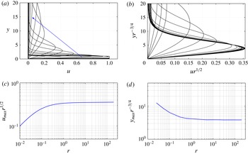
(a) Vertical profiles of the horizontal velocity
 $u$
at different values of
 ${\it\zeta}$
, as indicated below, for
 $j=0$
,
 ${\it\Lambda}=0$
,
 $Pr=0.7$
and
 ${\it\theta}_{f}=0$
. (b) The same profiles scaled with Glauert’s similarity variables (4.2). (c,d) Maximum of
 $u$
scaled with (4.2), and the scaled vertical location of this maximum, as functions of
 $r$
. (a)
 ${\it\zeta}=0.0003$
, 0.0014, 0.0028, 0.005, 0.025, 0.05, 0.1, 0.3, 0.6, 1, 3, 5, 10, 20, 30, 50, 70, 100, 130, 160, 200, increasing in the direction of the arrow.

4.2 Results for
 ${\it\Lambda}=0$

As already commented on, for
 ${\it\Lambda}=0$
with
 ${\it\theta}_{f}=0$
the solution must tend, far from the jet exit, to the similarity solution for the velocity field found by Glauert (Reference Glauert1956). This is checked here both for the 2D case and the axisymmetric case when
 $Pr=0.7$
. In our notation, the radial velocity field given by Glauert’s similarity solution can be written as
 $$\begin{eqnarray}u=A_{G}r^{-(j+1/2)}f_{G}^{\prime }({\it\tau}_{G}),\quad {\it\tau}_{G}=B_{G}\frac{y}{r^{(j+3/2)/2}},\end{eqnarray}$$
where
 $f_{G}$
satisfies equation (2.7) in (Glauert Reference Glauert1956) and
 $$\begin{eqnarray}A_{G}=\left\{\begin{array}{@{}lr@{}}{\displaystyle \frac{1}{4Re}}, & j=0\\ {\displaystyle \frac{3}{4Re^{3}}}, & j=1,\end{array}\right.\quad B_{G}=\left\{\begin{array}{@{}lr@{}}{\displaystyle \frac{1}{4Re^{1/2}}}, & j=0\\ {\displaystyle \frac{3}{4Re^{3/2}}}, & j=1.\end{array}\right.\end{eqnarray}$$
The corresponding non-dimensional skin friction at the wall is
 $$\begin{eqnarray}c_{f}=A_{G}B_{G}f_{G}^{\prime \prime }(0)r^{-(3j+5/2)/2}.\end{eqnarray}$$
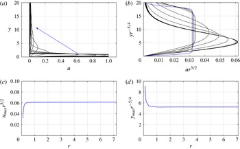
Figures 5(a) and 6(a) show some vertical profiles of the radial velocity as
 ${\it\zeta}$
increases for
 $j=0$
and
 $j=1$
with
 $R_{0}=0.1$
, respectively. Also shown (5
b and 6
b) are these velocity profiles scaled with the self-similar variables in (4.2), showing that they collapse into a single profile as
 $r$
increases. To better appreciate that the numerical solutions tend to Glauert’s similarity solution far away from the jet exit, we also plot in figures 5(c,d) and 6(c,d) the maximum radial velocity and its location conveniently scaled,
 $u_{max}r^{(j+1/2)}$
and
 $y_{max}r^{(j+3/2)/2}$
, as functions of
 $r$
. Note that the similarity solution is reached faster as
 $r$
increases in the axisymmetric case (
 $j=1$
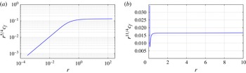
, figure 6), obviously due to the radial divergence of the flow. Finally, figure 7 shows the scaled skin friction
 $c_{f}r^{(3j+5/2)/2}$
as a function of
 $r$
for the same cases. All these quantities tend to constant values as
 $r$
increases, corroborating that Glauert’s self-similar solution is reached. The same happens for other values of
 $Pr$
and
 ${\it\theta}_{f}\neq 0$
.
As in figure 5, but for
 $j=1$
with
 $R_{0}=0.1$
: (a)
 ${\it\zeta}=0.0003$
, 0.0014, 0.0028, 0.005, 0.025, 0.05, 0.1, 0.3, 0.6, 1, 1.4, 1.6, 2.1, 2.3, 2.5, 2.9, 3.6, 4.8, 6, 7, increasing in the direction of the arrow.


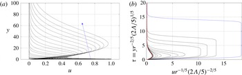
(a) Vertical profiles of
 $u$
at different values of
 ${\it\zeta}$
, as indicated below, for
 $j=0$
,
 ${\it\Lambda}=0.1$
,
 $Pr=0.7$
and
 ${\it\theta}_{f}=0$
. (b) The same profiles scaled with the similarity variables (3.9)–(3.10). Also included in (b) with a dashed (red) line is
 $f^{\prime }({\it\tau})$
for
 $j=0$
and
 $Pr=0.7$
from figure 2. (a)
 ${\it\zeta}=0.0003$
, 0.0014, 0.0028, 0.005, 0.025, 0.05, 0.1, 0.3, 0.6, 1, 3, 5, 10, 20, 30, 50, 80, 120, 170, 230, 300, 400, increasing in the direction of the arrow.

As in figure 8, but for the axisymmetric case (
 $j=1$
) with
 $R_{0}=0.1$
: (a)
 ${\it\zeta}=0.0003$
, 0.0014, 0.0028, 0.005, 0.025, 0.05, 0.1, 0.3, 0.6, 1, 3, 5, 10, 20, 30, 50, 80, 120, 170, 230, 300, 400, increasing in the direction of the arrow.

Evolution with
 $r$
of the friction coefficient at the wall
 $c_{f}$
scaled according to (3.14) for several values of the parameters, as indicated, all with
 $Pr=0.7$
.

4.3 Results for
${\it\Lambda}>0$

Figures 8 and 9 shows some vertical profiles of the horizontal velocity when
 ${\it\Lambda}=0.1$
(with
 $Pr=0.7$
and
 ${\it\theta}_{f}=0$
) for both the 2D case and the axisymmetric flow (with
 $R_{0}=0.1$
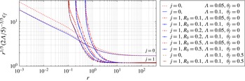
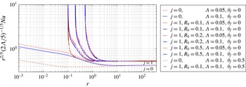
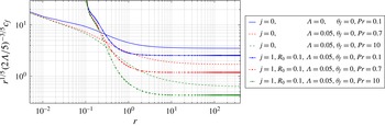
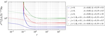
), respectively. It is observed that the velocity profiles collapse far from the jet exit to the similarity solution described in § 3 (when scaled appropriately). The same happens for the temperature profiles. But it is more instructive to show the local friction coefficient and Nusselt number written in the similarity variable (3.14), (3.15). This is done in figures 10 and 11, respectively, for
 $Pr=0.7$
, not only for the cases of figures 8 and 9, but for some other values of
 ${\it\Lambda}$
,
 ${\it\theta}_{f}$
, and
 $R_{0}$
. As predicted in § 3, the curves tend to asymptotic values as
 $r$
increases which are independent of
 ${\it\Lambda}$
,
 ${\it\theta}_{f}$
and
 $R_{0}$
(in the axisymmetric case), depending only on
 $j$
(when
 $Pr$
is fixed). Note that these asymptotes are reached much faster in the axisymmetric case than in the 2D flow. These figures include two cases with an inlet jet temperature different from the ambient temperature,
 ${\it\theta}_{f}=0.5$
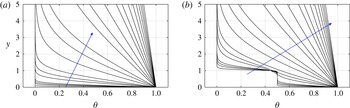
, one case for a 2D flow and the other one for a radial flow. In spite of the fact that the inlet conditions are very different, particularly for the temperature (see, for instance, figure 12, where we compare the temperature profiles for
 ${\it\theta}_{f}=0$
and
 ${\it\theta}_{f}=0.5$
in the 2D flow), both flows tend to the same corresponding similarity solution as
 $r$
increases, that only depends on
 $j$
when
 $Pr$
is fixed. Note that
 $c_{f}(r)$
is hardly modified by the different inlet temperatures, especially for
 $j=1$
(figure 10), but
 $Nu(r)$
for
 ${\it\theta}_{f}=0$
and
 ${\it\theta}_{f}=0.5$
are quite different (figure 11) due to the very different initial temperature profiles (see figure 12), until reaching the common asymptote. Similar behaviours are found for inlet temperatures higher than the ambient temperature,
 ${\it\theta}_{f}>1$
, not shown.
Evolution with
 $r$
of the local Nusselt number scaled according to (3.15) for several values of the parameters, as indicated, all with
 $Pr=0.7$
.

Vertical profiles of
 ${\it\theta}$
at different values of
 ${\it\zeta}$
, as indicated below, for
 $j=0$
,
 ${\it\Lambda}=0.1$
,
 $Pr=0.7$
,
 ${\it\theta}_{f}=0$
(a) and
 ${\it\theta}_{f}=0.5$
(b): (a,b)
 ${\it\zeta}=0.0003$
, 0.0014, 0.0028, 0.005, 0.025, 0.05, 0.1, 0.3, 0.6, 1, 3, 5, 10, 20, 30, 50, 80, 120, 170, 230, 300, 400, increasing in the direction of the arrow.

Evolution with
 $r$
of the friction coefficient at the wall
 $c_{f}$
scaled according to (3.14) for several values of
 $Pr$
at selected values of the remaining parameters, as indicated.

Evolution with
 $r$
of the local Nusselt number scaled according to (3.15) for several values of
 $Pr$
at selected values of the other parameters, as indicated.

Figures 13–14 show
 $c_{f}$
and
 $Nu$
for different values of
 $Pr$
at selected values of the other parameters. In agreement with the analytical results in § 3, the asymptotic value of the friction coefficient for
 $r\gg 1$
decreases with increasing
 $Pr$
, all the remaining parameters the same, being larger for the 2D flow (
 $j=0$
) than for the radial flow (
 $j=1$
). In contrast, the Nusselt number increases with
 $Pr$
, being larger for the axisymmetric case than for the 2D flow.
5 Summary and conclusion
A similarity solution for the wall jet over a heated horizontal plate at constant temperature that takes into account the coupling of temperature and velocity fields through buoyancy has been described. For a given temperature difference between the plate and the ambient,
 $T_{0}-T_{a}$
, a vertical scale length
 ${\it\delta}$
, and a characteristic horizontal velocity
 $U$
, this coupling is quantified by the dimensionless parameter
 ${\it\Lambda}={\it\beta}g{\it\delta}(T_{0}-T_{a})/U^{2}=Gr/Re^{2}$
, where
 $Re$
and
 $Gr$
are the corresponding Reynolds and Grashof numbers, respectively.
 ${\it\Lambda}$
is also equivalent to the inverse of a Froude number. For
 ${\it\Lambda}=0$
one has the well-known Glauert’s (Reference Glauert1956) similarity solution for a wall jet without buoyancy. But this solution is qualitatively very different from the one found here for
 ${\it\Lambda}>0$
in two main aspects. First, Glauert’s similarity variable is
 ${\it\tau}_{G}\propto y/r^{(j+3/2)/2}$
, while for
 ${\it\Lambda}\neq 0$
we find
 ${\it\tau}\propto y/r^{2/5}$
, both for the 2D flow (
 $j=0$
) and for the axisymmetric, or radially spreading, flow (
 $j=1$
). Thus, the basic structure of the similarity flow is the same for the planar and the radial flow, and very different from the two distinct flow structures in Glauert’s similarity solution. Second, the radial or horizontal velocity increases with
 $r$
as
 $u\propto r^{1/5}$
, both for the 2D flow and for the axisymmetric flow, while in Glauert’s solution it decays as
 $u_{G}\propto r^{-(j+1/2)}$
. In addition, the radial dependence of the temperature field differs from the one associated to Glauert’s flow. The similarity solution described here is also qualitatively different from the one found by Stewartson (Reference Stewartson1958) for the purely free convection flow over a horizontal plate because no characteristic velocity exists in this last problem, so that no equivalent to the parameter
 ${\it\Lambda}$
, or to a Froude number, exists. Also, only the two-dimensional (
 $j=0$
) flow was considered by Stewartson.
Parameter
 ${\it\Lambda}$
is embedded into the similarity solution, so that the dependence with
 ${\it\Lambda}$
of the velocity and temperature fields and, consequently, of the skin friction and heat flux at the wall, are given explicitly. In particular, the friction coefficient and Nusselt number behave as
 $$\begin{eqnarray}c_{f}\propto {\it\Lambda}^{3/5}r^{-1/5},\quad Nu\propto {\it\Lambda}^{1/5}r^{-2/5},\end{eqnarray}$$
both for the 2D flow and for the axisymmetric flow. Simple correlations for the proportionality constants in (5.1) as functions of the Prandtl number
 $Pr$
are given for
 $j=0$
and
 $j=1$
.
To check the validity of this similarity solution we have solved numerically the boundary layer flow emerging radially with uniform velocity
 $U$
and temperature
 $T_{f}$
from a circular slot of radius
 $r_{0}$
and height
 ${\it\delta}$
over a plate at constant temperature
 $T_{0}$
and into an ambient fluid at rest with temperature
 $T_{a}$
. In addition to
 ${\it\Lambda}$
, the problem is governed by the dimensionless parameters
 $Pr$
,
 ${\it\theta}_{f}$
(
 $\neq 0$
if
 $T_{f}\neq T_{a}$
), and, in the axisymmetric case,
 $R_{0}$
, related to
 $r_{0}$
. A self-similar solution valid near the jet exit is also provided in this work, which in addition serves to initiate the numerical integration of the boundary layer equations towards the far-field solution. We have checked that the similarity solution is reached far from the jet exit for all the values of
 $j$
,
 $Pr$
,
 ${\it\theta}_{f}$
and
 $R_{0}$
investigated, provided that
 ${\it\Lambda}>0$
, i.e.
 $T_{0}>T_{a}$
. For
 ${\it\Lambda}<0$
(cooled plate), the far-field similarity solution does not exist, as is clear from its structure (e.g. (5.1)), and as previously reported in related mixed-convection flows over a cooled plate at constant temperature (Schneider & Wasel Reference Schneider and Wasel1985; Steinrück Reference Steinrück1994, Reference Steinrück1995; Higuera Reference Higuera1997). We find numerically that the boundary layer solution for
 ${\it\Lambda}<0$
always breaks down at a finite streamwise distance from the jet exit because reverse flow is originated within the boundary layer due to the adverse pressure gradient induced by buoyancy when
 ${\it\Lambda}<0$
, and a similarity solution is never attained. In all the cases with
 ${\it\Lambda}<0$
that we have explored numerically, reverse flow inside the boundary layer is first originated at some distance from the wall, so that the skin friction
 $c_{f}$
does not vanish at, or just before, the failure of the numerical scheme. On the other hand, no terminal singularity of the skin friction like that described by Daniels (Reference Daniels1992) and Daniels & Gargaro (Reference Daniels and Gargaro1993) for a horizontal insulated surface has been found in the present problem. We suspect that in the axisymmetric case (
 $j=1$
), and for sufficiently small
 $R_{0}$
, the boundary layer solution also breaks down as
 $r$
increases above a threshold value of
 ${\it\Lambda}>0$
, and the similarity solution is not reached, but we have not explored this possibility in the present work. For
 ${\it\Lambda}=0$
Glauert’s similarity solution is recovered for any set of values of the remaining parameters investigated.
Appendix A. Approximate solution near the jet exit
An approximate solution for small
 ${\it\zeta}\equiv r-j\,R_{0}$
which is of interest not only from a theoretical point of view, but also to start the numerical integration of the parabolic equations (2.2)–(2.4), is obtained here. At its lowest order in powers of
 ${\it\zeta}$
this solution is composed by the self-similar Blasius solution near
 $y=0$
plus the self-similar solution for a plane half-jet near
 $y=1$
(see, e.g. Schlichting & Gersten Reference Schlichting and Gersten2000). In particular, for
 ${\it\zeta}\ll 1$
and
 ${\it\zeta}\ll R_{0}$
(in the axisymmetric case), one may write (3.1), in first approximation, as
 $$\begin{eqnarray}u\simeq \left(1-j\frac{{\it\zeta}}{R_{0}}\right)\frac{\partial {\it\psi}}{\partial y},\quad v\simeq -\left(1-j\frac{{\it\zeta}}{R_{0}}\right)\frac{\partial {\it\psi}}{\partial {\it\zeta}},\end{eqnarray}$$
where the constant
 $R_{0}^{-j}$
has been absorbed into
 ${\it\psi}$
. As
 ${\it\zeta}\rightarrow 0$
,
 $\sqrt{{\it\zeta}}\,{\it\psi}$
and
 ${\it\theta}$
are functions of Blasius’ similarity variable
 $$\begin{eqnarray}{\it\tau}_{0}=\frac{y}{\sqrt{{\it\zeta}}},\end{eqnarray}$$
for
 $y\ll 1$
, while they are functions of
 $$\begin{eqnarray}{\it\tau}_{1}=\frac{y-1}{\sqrt{{\it\zeta}}},\end{eqnarray}$$
for
 $|y-1|\ll 1$
(Lessen Reference Lessen1949). Thus, close to
 $y=0$
and
 $y=1$
one may use the following expansions for
 ${\it\zeta}\ll 1$
:
 $$\begin{eqnarray}{\it\psi}_{i}={\it\zeta}^{1/2}f_{i0}({\it\tau}_{i})+{\it\zeta}f_{i1}({\it\tau}_{i})+\cdots \,,\end{eqnarray}$$
 $$\begin{eqnarray}{\it\theta}_{i}={\it\theta}_{i0}({\it\tau}_{i})+{\it\zeta}^{1/2}{\it\theta}_{i1}({\it\tau}_{i})+\cdots \,,\end{eqnarray}$$
with
 $i=0$
and
 $i=1$
, respectively. Substituting these expansions into (2.3)–(2.4) one obtains, for the two first terms in the expansion,
 $$\begin{eqnarray}f_{i0}^{\prime \prime \prime }+{\textstyle \frac{1}{2}}\,f_{i0}\,f_{i0}^{\prime \prime }=0,\end{eqnarray}$$
 $$\begin{eqnarray}{\it\theta}_{i0}^{\prime \prime }+\frac{Pr}{2}\,f_{i0}\,{\it\theta}_{i0}^{\prime }=0,\end{eqnarray}$$
 $$\begin{eqnarray}f_{i1}^{\prime \prime \prime }+\frac{1}{2}f_{i0}f_{i1}^{\prime \prime }-\frac{1}{2}f_{i0}^{\prime }f_{i1}^{\prime }+f_{i0}^{\prime \prime }f_{i1}=-\frac{{\it\Lambda}}{2}\left[{\it\tau}_{i}({\it\theta}_{i0}-{\it\theta}_{f})+\int _{{\it\tau}_{i}}^{\infty }{\it\theta}_{i0}\,\text{d}{\it\tau}_{i}\right],\end{eqnarray}$$
 $$\begin{eqnarray}{\it\theta}_{i1}^{\prime \prime }+Pr\left(f_{i1}{\it\theta}_{i0}^{\prime }+{\textstyle \frac{1}{2}}\,f_{i0}{\it\theta}_{i1}^{\prime }-{\textstyle \frac{1}{2}}\,f_{i0}^{\prime }{\it\theta}_{i1}\right)=0,\end{eqnarray}$$
for
 $i=0$
and
 $i=1$
, where the primes denote differentiation with respect to the corresponding
 ${\it\tau}_{i}$
. These equations have to be solved with the following boundary conditions:
for
 $i=0$
,
 $$\begin{eqnarray}f_{00}(0)=f_{00}^{\prime }(0)=0,\quad {\it\theta}_{00}(0)=1,\quad f_{00}^{\prime }(\infty )=1,\quad {\it\theta}_{00}(\infty )={\it\theta}_{f},\end{eqnarray}$$
 $$\begin{eqnarray}f_{01}(0)=f_{01}^{\prime }(0)={\it\theta}_{01}(0)=0,\quad f_{01}^{\prime }(\infty )={\it\theta}_{01}(\infty )=0;\end{eqnarray}$$
for
 $i=1$
,
 $$\begin{eqnarray}f_{10}({\it\tau}_{1}\rightarrow -\infty )\rightarrow f_{00}(\infty )+{\it\tau}_{1},\quad f_{10}^{\prime }(-\infty )=1,\quad {\it\theta}_{10}(-\infty )={\it\theta}_{f},\end{eqnarray}$$
 $$\begin{eqnarray}f_{10}^{\prime }(\infty )=0,\quad {\it\theta}_{10}(\infty )=0,\end{eqnarray}$$
 $$\begin{eqnarray}f_{11}(-\infty )=f_{01}(\infty ),\quad f_{11}^{\prime }(-\infty )={\it\theta}_{11}(-\infty )=0,\quad f_{11}^{\prime }(\infty )={\it\theta}_{11}(\infty )=0.\end{eqnarray}$$
First one solves the equations for
 ${\it\tau}_{0}$
, and then those for
 ${\it\tau}_{1}$
using the obtained values
 $f_{00}(\infty )$
and
 $f_{01}(\infty )$
in the boundary conditions (A 13)–(A 14).
Note that with just these two terms in the expansions, first-order buoyancy effects are taken into account through the second term, but one does not see the radial divergence of the flow in the axisymmetric case. This radial effect enters at the next order (third term) in the expansions (A 4)–(A 5) in powers of
 ${\it\zeta}$
(Fernandez-Feria et al.
Reference Fernandez-Feria, del Pino and Fernandez-Gutierrez2014). But the above two terms are enough to start with accuracy the numerical integration of equations (2.2)–(2.11a,b
). Actually, one uses as initial conditions a composite self-similar solution, which is obtained adding the terms for
 $i=0$
and for
 $i=1$
and subtracting the common terms as
 ${\it\tau}_{0}\rightarrow \infty$
and
 ${\it\tau}_{1}\rightarrow -\infty$
, respectively. In particular, we use the following initial conditions at a given
 $r_{in}={\it\zeta}_{in}+jR_{0}$
,
 ${\it\zeta}_{in}\ll 1$
, to solve (2.2)–(2.11a,b
) numerically:
 $$\begin{eqnarray}u_{in}(y)\equiv u(r_{in},y)=f_{00}^{\prime }({\it\tau}_{0in})+{\it\zeta}_{in}^{1/2}f_{01}^{\prime }({\it\tau}_{0in})+f_{10}^{\prime }({\it\tau}_{1in})+{\it\zeta}_{in}^{1/2}f_{11}^{\prime }({\it\tau}_{1in})-1,\end{eqnarray}$$
 $$\begin{eqnarray}\displaystyle v_{in}(y) & \equiv & \displaystyle v(r_{in},y)=-{\textstyle \frac{1}{2}}{\it\zeta}_{in}^{-1/2}\left[f_{00}({\it\tau}_{0in})-{\it\tau}_{0in}f_{00}^{\prime }({\it\tau}_{0in})\right]-f_{01}({\it\tau}_{0in})+{\textstyle \frac{1}{2}}{\it\tau}_{0in}f_{01}^{\prime }({\it\tau}_{0in})\nonumber\\ \displaystyle & & \displaystyle -\,{\textstyle \frac{1}{2}}{\it\zeta}_{in}^{-1/2}\left[f_{10}({\it\tau}_{1in})-{\it\tau}_{1in}f_{10}^{\prime }({\it\tau}_{1in})\right]-f_{11}({\it\tau}_{1in})+{\textstyle \frac{1}{2}}{\it\tau}_{1in}f_{11}^{\prime }({\it\tau}_{0in})+{\textstyle \frac{1}{2}}{\it\zeta}_{in}^{-1/2}f_{00}(\infty )\nonumber\\ \displaystyle & & \displaystyle +\;f_{01}(\infty ),\end{eqnarray}$$
 $$\begin{eqnarray}{\it\theta}_{in}(y)\equiv {\it\theta}(r_{in},y)={\it\theta}_{00}^{\prime }({\it\tau}_{0in})+{\it\zeta}_{in}^{1/2}{\it\theta}_{01}^{\prime }({\it\tau}_{0in})+{\it\theta}_{10}^{\prime }({\it\tau}_{1in})+{\it\zeta}_{in}^{1/2}{\it\theta}_{11}^{\prime }({\it\tau}_{1in})-{\it\theta}_{f},\end{eqnarray}$$
where
 ${\it\tau}_{0in}=y/\sqrt{{\it\zeta}_{in}}$
and
 ${\it\tau}_{1in}=(y-1)/\sqrt{{\it\zeta}_{in}}$
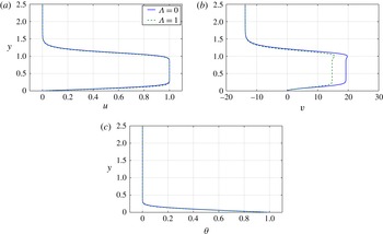
. Figure 15 shows these initial profiles for
 ${\it\zeta}_{in}=2\times 10^{-3}$
in some particular cases. Since the radial divergence effect is not accounted for in the present approximation with just two terms in the expansions (A 4)–(A 5), these initial profiles are independent of
 $j$
and, consequently, of
 $R_{0}$
. Note also than for
 ${\it\Lambda}=0$
the second correction in the expansion for
 ${\it\zeta}\ll 1$
vanish, so that the continuous lines in figure 15 for
 ${\it\Lambda}=0$
coincide with the lowest order of the expansion for
 ${\it\Lambda}\neq 0$
. Finally, it is worth mentioning that
 $v$
is always negative as
 $y\rightarrow \infty$
. This is a consequence of the fact that both
 $u$
and
 ${\it\theta}$
vanish as
 $y\rightarrow \infty$
: if
 $v_{\infty }(r)\equiv v(r,y\rightarrow \infty )$
, the solution of (2.4) as
 $y\rightarrow \infty$
that satisfies the boundary condition at infinity behaves as
 ${\it\theta}\sim C(r)\exp [Pr\,v_{\infty }y]$
, implying that
 $v_{\infty }(r)<0$
for any
 $r$
. Similarly, (2.3) implies that the leading term of
 $u$
as
 $y\rightarrow \infty$
behaves as
 $u\sim K_{1}(r)y\exp [Pr\,v_{\infty }y]$
or as
 $u\sim K_{2}(r)\exp [v_{\infty }y]$
, depending on whether
 $Pr$
is larger or smaller than unity, respectively, with
 $K_{1}(r)$
related to
 $C(r)$
. In both cases
 $v_{\infty }(r)$
should be negative for any
 $r$
.