
Do the economic effects of international trade influence who wins the US presidency? The expansion of trade has produced favorable employment conditions for firms producing high-skilled tradable goods (e.g., petrochemical manufacturing) and services (e.g., software) because the United States has a comparative advantage in these activities. Likewise, trade has led to increased competition and unfavorable employment conditions for firms producing low-skilled goods (e.g., apparel). Building on research demonstrating that economic conditions explain support for incumbent presidents and their parties,Footnote 1 we expect citizens to cast their votes for president in part based upon their employment exposure—either favorable or unfavorable—to trade. Employees in high-wage tradable goods and services sectors are more likely to support incumbent presidents and their parties, whereas those in low-wage manufacturing jobs will be more likely to support the opposition. Examining county-level election results from 1992 to 2012 and national-level results beginning in 1936, we find strong support for our argument: voters' exposure to trade influences who wins the US presidency.
Our primary contribution is to examine both the favorable and unfavorable effects of trade exposure on US presidential elections. We develop novel comprehensive measures of trade exposure in goods and services using US Census data covering nearly all economic activity in the United States. Including trade-exposed service workers in the analysis is important for three reasons. First, the manufacturing sector's share of employment has been in secular decline for decades, and now accounts for less than 10 percent of the labor force. Because of data limitations on services trade, prior studies necessarily focused on the electoral consequences of goods trade competition.Footnote 2 However, those working in tradable goods are a declining portion of the electorate. Second, trade in services is increasing, and now accounts for 30 percent of US exports. Casual observation and recent studies suggest that trade in services significantly increases the trade exposure of the US economy.Footnote 3 Third, tradable services have qualitatively different factor demands: they are significantly more skill intensive than either the manufacturing sector or nontradable services.Footnote 4 The United States remains a relatively skill-abundant country—it should have a comparative advantage in skill-intensive industries. The persistent and growing trade surplus in services demonstrates its comparative advantage in this sector.
The consideration of tradable service workers enables us to identify those who are likely to gain from increased trade, and to better isolate trade's impact on trade-exposed manufacturing workers who are likely to lose from increased international competition.Footnote 5 We are thus able to determine the types of firms, industries, and locations that benefit—or are displaced by—increased economic integration. We estimate how county-level variation in employment in firms in comparatively advantaged and disadvantaged sectors affects voting in US presidential elections. County-level data also allow us to aggregate results by states. We compare the estimated results in swing states (in which the outcomes of US presidential elections are generally determined) to those of non-swing states.
We find that more workers in high-skilled exportable services and high-skilled exportable manufacturing are associated with increasing incumbent party vote shares. To our knowledge, we are the first to demonstrate that increasing employment in high-skilled industries is associated with increasing support for incumbents. We confirm Margalit's finding that manufacturing losses harm incumbent vote shares over an extended period (1996–2012).Footnote 6 Examining the crucial swing states, we find that the negative effect of comparatively disadvantaged manufacturing employment on incumbent vote shares is approximately three times as large as in non-swing states, which leads to a powerful Electoral College incentive to protect this sector. We also study, to our knowledge for the first time, the effects of trade in established US national-level election models from the American politics literature. Our results indicate that voters punish (reward) the incumbent party against a backdrop of rising imports (exports).
This paper contributes most directly to a nascent literature on the effects of trade on voting. Building on recent research demonstrating that the employment dislocations and wage adjustments from trade are larger and more long lasting than previously thought,Footnote 7 the trade and voting literature has focused on the effects of increasing import competition on citizen voting preferences.Footnote 8 This work finds that import shocks influence voting in congressional and presidential elections. With the exception of Margalit, the existing research focuses exclusively on the electoral consequences of manufacturing import competition from China. Our paper extends the research by considering the voting activities of trade's potential winners as well as losers.
By focusing on trade's varied distributional consequences, we contribute more broadly to a large literature examining how firms' and individuals' exposure to the global economy affects support for trade. Prior work demonstrates that firms' demands for trade protection (or liberalization) depend on their international integration through global supply chains and trade patterns,Footnote 9 or as a result of industry characteristics such as the degree of exchange rate pass-through to prices,Footnote 10 global sourcing,Footnote 11 and product differentiation.Footnote 12 Evidence from survey data finds that the globalization of production increases wage and employment volatility, leading workers to feel economically insecure.Footnote 13 To date, the impact of employment in comparatively advantaged sectors on voter support for incumbent presidents has not been explored.
Our paper also relates to studies examining how the subnational distribution of economic activity in comparatively advantaged and disadvantaged sectors influences trade policy-making. Following Rogowski, who argues that political divisions over trade reflect factor-based distributional concerns,Footnote 14 a number of studies link the expected winners and losers of global trade and financial flows to US international economic policy-making in Congress. Hiscox finds that legislator support for trade between 1824 and 1994 reflects the expected gains and losses experienced by class- and industrial-based constituencies.Footnote 15 Other studies examine how industry structure at the district level, which proxies for concentrations of voters with similar economic interests, influences legislator voting on trade and other international economic policy-making issues.Footnote 16 Districts with concentrations of high-skilled voters are associated with greater legislator support for trade.Footnote 17 Representatives from districts affected by import competition from ChinaFootnote 18 and those representing higher concentrations of offshorable employmentFootnote 19 vote in a more protectionist manner. If trade has the distributional consequences implied by these studies, voters who are harmed by (benefit from) trade will be more likely to shift away from (toward) the incumbent or the incumbent's party.
US Trade Integration, Economic Attribution, and Presidential Voting
We draw on a long tradition in the American politics literature investigating how economic conditions affect voting. These established national-level (macro) studies show that voters are more likely to reward incumbent presidents and their parties during good economic times, and to reward the opposition when economic conditions deteriorate.Footnote 20 Starting with the Fair and Tufte models, scholars have empirically demonstrated that positive economic performance strongly improves either incumbent or incumbent party re-election prospects.Footnote 21
The macro voting models are necessarily concise, however, because of the few degrees of freedom involved in the data, and have yet to include trade variables explicitly.Footnote 22 Invariably, macro models assume that certain aspects of economic performance are the key determinants of incumbent support: economic growth,Footnote 23 disposable income, employment, job growth,Footnote 24 and business sentimentFootnote 25 are contending variables. Quinn and Woolley show that economic volatility drives down vote shares for incumbent candidates and parties in a comparative, cross-national setting.Footnote 26 Given the few degrees of freedom and the many competing plausible correlates of incumbent vote shares, it is not surprising that trade variables have so far been omitted from the discussion.
We expect that voters will hold incumbents of both major US political parties responsible for trade outcomes, with incumbents gaining or losing votes from gains or losses in trade balances (respectively).Footnote 27 This is because, as Destler shows, all presidents since 1936 have supported trade liberalization to one degree or another.Footnote 28 This is in contrast to Congressional trade politics, where Democrats from the mid-1990s onward began to oppose trade liberalization.Footnote 29
While the macro studies have neglected the direct impact of trade on voting outcomes, several recent studies examining subnational election results find that trade's distributional effects influence how people vote. Examining county-level election results, Margalit demonstrates that job loss from import competition—measured as applications for Trade Adjustment Assistance (TAA)—had a negative aggregate effect on county-level presidential voting in the 2004 election.Footnote 30 Studying the specific impact of economic shocks from Chinese import competition, Feigenbaum and Hall find that legislators from exposed districts vote in a more protectionist manner,Footnote 31 while Autor and colleagues find increased polarization in US congressional districts.Footnote 32 Che and colleagues show that counties facing more competition from China are more likely to elect House Democrats, and that these Democratic House members are more likely to oppose free trade legislation.Footnote 33 These studies are persuasive in demonstrating that foreign competition affects electoral and other outcomes, although trade exposure in low-skilled manufacturing is unlikely to be the only channel through which international integration influences voting behavior.
However, the increasing global integration of an economy might diminish voter attribution of responsibility to incumbent parties under some circumstances. Hellwig and Samuels demonstrate that, among democratic countries generally, the effects of economic voting on incumbent vote shares diminish with the increasing exposure of an economy to economic globalization.Footnote 34 Kayser and Peress decompose economic growth for a panel of countries into domestic and exogenous (international shock) components, and find the voters punish incumbents for national performance that lags international performance, but not economic performance per se.Footnote 35
These studies also find that US voters are among the global voters most likely to attribute responsibility for economic performance to incumbent policy-makers. The United States in the period examined here is one of the least economically open advanced industrial countries examined by Hellwig and Samuels.Footnote 36 For the US, economic growth is associated with increasing incumbent vote shares.Footnote 37 Hellwig found that US respondents overwhelmingly attributed to either Congress or the president responsibility “for national economic conditions.”Footnote 38 Kayser and Peress, in turn, exclude the US from their study of voter attribution of economic performance because, unlike their foreign counterparts, US policy-makers continue to exert strong influence on US economic conditions.Footnote 39 We therefore expect US voters to hold incumbents electorally accountable for economic conditions.
Our argument emphasizes how a voter's position in the global economy may influence her support for the incumbent party. The logic that we develop does not require that voters possess a sophisticated understanding of the distributional implications of trade. Indeed, recent work suggests that voters' knowledge about the general effects of trade on employment and wages is quite low.Footnote 40 Voters' trade policy preferences—which we do not explicitly examine—may be shaped by nonmaterial objectives.Footnote 41
We propose two modifications to the existing literature. We argue and demonstrate at the county-level using newly available measures of trade exposure in services that trade's likely winners—workers employed in tradable, high-skilled industries—are more likely to vote for incumbents and their parties. That is, we explore the electoral consequences of the gains, as well as the losses, from US trade exposure. Because our argument has national as well as subregional implications, we also extend the national-level voting models to include trade indicators, including changes in imports and exports.
Our local- and national-level analyses provide a more comprehensive picture of the relationship between trade and US presidential voting. The county-level analyses allow for finer-grained insights regarding economic conditions, and for the incorporation of precisely estimated measures of citizen exposure to trade. The disadvantage of the county-level data is that only six elections can be considered. The national-level models, while offering less precision and fewer degrees of freedom, allow for the consideration of direct trade flows and a greater number of elections (back to 1936). The results from multiple levels of analysis provide strong and consistent evidence that citizen exposure to trade influences US presidential elections.
The Possible Effects of Trade Integration on US Presidential Voting
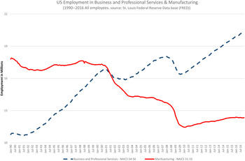
Service sector trade exposure may influence voting behavior in US elections. Our emphasis on the services sector is based on three facts. First, the service sector is large, accounting for at least half and, depending on how it is defined, upwards of 80 percent of the US labor force.Footnote 42 (In contrast, the manufacturing sector is a relatively small share of the labor force—accounting for less than 10 percent in 2012.) Figure 1 shows the changing levels of employment in two broad categories of employment that are largely tradable—manufacturing (which is defined as NAICS 31–33) and business and professional services (BPS, which is defined as NAICS 54–56). The figure indicates that employment in BPS has nearly doubled since 1990, whereas manufacturing employment has contracted by nearly a third.Footnote 43 If even some relatively small portion of the service sector is trade exposed, increased international integration potentially affects a larger number of service jobs than manufacturing jobs.
Changing composition of US employment, 1990–2016

Second, while services were traditionally considered to be largely nontradable, the “tradability” of the service sector has increased markedly with technological changes and financial current-account liberalizations that make trade in intangibles, such as intellectual property, possible.Footnote 44 Services accounted for 33 percent of the value of US exports in the first quarter of 2016.Footnote 45
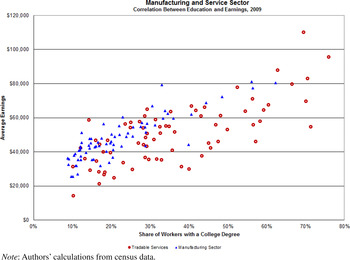
Third, tradable services are more skill intensive than both nontradable services and the manufacturing sector. Jensen and coauthors report that tradable services are significantly more skill intensive (as measured by educational attainment or average earnings) than service industries classified as nontradable and the manufacturing sector.Footnote 46 Because tradable services differ in the intensity of their use of high-skilled labor relative to other sectors, they are likely to face different levels of competition and different levels of opportunity from increased international integration. Heckscher-Ohlin (HO) trade theory suggests that countries with an abundant factor will have a comparative advantage in industries that make intensive use of that factor.Footnote 47 The United States is still skill abundant vis-à-vis the rest of the world—suggesting that it should have comparative advantage in skill-intensive activities like tradable services. The United States' persistent and growing trade surplus in services is evidence that it indeed has a comparative advantage in services (in stark contrast to its large and persistent trade deficit in goods).Footnote 48
Because the United States is a relatively high-skill-abundant country, it has a comparative advantage in high-skilled activities and a comparative disadvantage in low-skilled activities. Jensen argues that tradable business service activities are consistent with US comparative advantage, and that therefore firms and workers in high-skilled tradable service activities will benefit from the increased tradability of services.Footnote 49 By contrast, firms in low-skill, labor-intensive tradable manufacturing industries tend to face greater import competition, particularly as trade agreements have brought previously trade-isolated countries, especially China, into the global economy.Footnote 50 The differential effects of trade exposure on workers in these two tradable sectors suggest that workers' voting behaviors will differ.
The differences in the effects of trade exposure are compounded by differences in wage premia across sectors. Previous empirical literature strongly suggests that workers with similar skills receive higher wages in the manufacturing sector than in the service sector.Footnote 51 Because that wage premium is significantly reduced if the worker leaves the sector, workers in the manufacturing sector suffer greater harm when being displaced from their jobs compared to workers in the service sector.
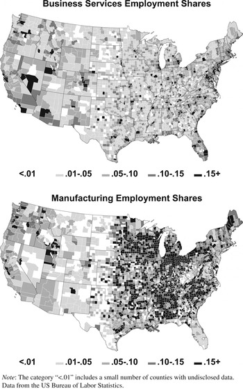
The differences in worker trade exposure in services versus manufacturing are potentially amplified by the geographic concentrations of industrial production. As can be seen in the upper panel of Figure 2, workers in business services, many of which are tradable, are concentrated in urban areas and on the East and West coasts. In contrast, the lower panel of Figure 2 shows that manufacturing workers tend to be concentrated in midwestern and southern states, many of which are “swing” states. As Autor and colleagues note, population movements are “sluggish,”Footnote 52 and as we proposed earlier that worker transitions between sectors have wage costs, we expect modest movement geographically and sectorally. We will thus explore possible differences between swing and non-swing states.
Proportional employment shares (0–1.0) in 2012 by county

We expect that employees' votes will reflect their experiences of their industries', their employers', and their own economic circumstances. Employees in firms producing in comparatively disadvantaged tradable sectors, especially low-skilled employees, experience directly that their jobs are internationally contestable and are thus vulnerable to increased trade competition—even before job losses or gains are reflected in the unemployment rate. In contrast, employees of firms in industries in which the United States has a comparative advantage, especially employees who are highly skilled, experience directly the benefits of US trade integration, including increased demand for their skills, or increased demand for the services provided by their firm.
Measuring Tradable Services
If employment in tradable services is higher than in the manufacturing sector, and if the workers employed in tradable services are qualitatively different from those in the manufacturing sector, then tradable service workers may influence elections differently than manufacturing workers do. To empirically investigate this possibility, we need to identify employment in tradable services.
While we would ideally use statistics on international trade in service flows to identify tradable and traded services (as can be done for trade in manufacturing), the US trade-in-services data, which are collected by the US Bureau of Economic Analysis (BEA), are inadequate for our purposes. An important shortcoming of the BEA trade-in-services data is that, in contrast with merchandise trade statistics that are produced for 10,000 manufacturing product categories—allowing detailed identification of the trade exposure of individual manufacturing industries—service trade data are available for about only thirty categories (beginning in 2006). Prior to that year, fewer than twenty categories are available for trade in services. The highly aggregated categories of services trade are therefore certainly combining tradable and nontradable industries into the same category, making identification of exposed industries difficult.Footnote 53
Another shortcoming is that the BEA data are believed to understate the size of trade in services because official BEA trade statistics are potentially missing a significant share of service trade. Since services do not pass through ports (as merchandise does), the data collection system for international trade-in-services statistics relies on surveys instead of customs forms. Relatively small budgets for service trade data collection and very high service trade reporting thresholds suggest that the services trade is not well measured.Footnote 54
Given these data limitations for trade in services, we instead identify variation in tradability among disaggregated industries within the manufacturing and services sectors by adapting the methodology developed by Jensen and KletzerFootnote 55 who classify industry tradability according to the geographic concentration of the six-digit NAICS industry in the United States. They make the assumption that when production exceeds local demand, the excess supply must be consumed elsewhere—that is, exported to another region.Footnote 56 For example, grocery stores are distributed throughout the United States in proportion to population. For grocery stores, trade costs are high so local demand is served by local production: low concentration implies low tradability. In contrast, software production is highly concentrated in Silicon Valley and Seattle. In software, trade costs are low, so production is concentrated in a few regions and shipped around the country (and around the world). This intuition can be applied to goods as well as services, and allows us to construct consistent measures for the whole economy.
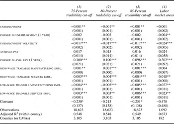
In particular, we use the Gini coefficient of the geographic concentration of production above what would be predicted by local demand to identify tradable industries.Footnote 57 Since we have a good understanding of the tradability of manufactured goods, we use the manufacturing sector as the basis for setting the cut-off for the geographic concentration Gini that signifies tradability. We define the tradability cut-off as the Gini coefficient that classifies 90 percent of manufacturing sector employment being tradable.Footnote 58 We use the same Gini coefficient as the tradability cut-off for the service sector. If the Gini coefficient for a service industry is above the threshold that results in 90 percent of manufacturing sector employment being classified as tradable, that industry is classified as tradable. (We also applied cut-offs of 75, 80, and 85 percent, and obtained substantively identical results. See Appendix Table A1, models 1, 2, and 3.)Footnote 59
We adopt the definition of services trade defined by balance-of-payments accounting conventions and the World Trade Organization's General Agreement on Trade in Services (GATS).Footnote 60 These include cross-border exports (“Mode 1”), services consumption abroad (“Mode 2”), a commercial presence abroad (“Mode 3”), and foreign services contractors abroad (“Mode 4”). For services, our measure of tradability, which is based on the geographic concentration of production in the United States, captures the employment impact of Modes 1, 2, and 4.Footnote 61
Tradability under GATS differs from the concept of offshorability, which relates to the ability to perform work from abroad.Footnote 62 Not all tradable services and not all tradable manufacturing jobs are offshorable.Footnote 63 For instance, tradable service industries include US-based tourism-related industries. (For example, Disney World is an exporter of amusement park services under the Balance of Payments Manual classification when nonresidents “consume” this amusement park service.) Most manufacturing jobs require workers to be physically present in an establishment to complete a job, implying tradability of the product, but not always the offshorability of the manufacturing job.Footnote 64
Table 1 provides examples of industries that we classify as tradable and nontradable, high skilled and low skilled, in manufacturing and services. The results are intuitively appealing. The manufacturing industries classified as tradable are well-known examples of manufacturing industries that are geographically concentrated and traded. Those classified as nontradable—corrugated boxes, cement, and quick printing—all have high transport cost-to-value ratios. In these industries, production is distributed throughout the United States and international trade shares are low.
Industry classifications by tradability, product, and skill

Note: Authors' calculations using Economic Census data.
The service industries are also intuitively appealing. Computer system design services, investment banking, and software publishing are all highly tradable and geographically concentrated in the United States. The same is true for credit card issuing, amusement parks, and limousine services. The latter two are tourism-related industries that are geographically concentrated; they are examples of Mode 2 trade, serving customers from all over the world. The nontradable service industries make sense as well. Restaurants, dentist offices, and grocery stores all have high trade costs relative to value. Production in these industries is distributed throughout the country.
In addition to tradability, we also expect that skill intensity is an important dimension for trade exposure. High-skill-intensive activities are consistent with US comparative advantage, and thus the United States should specialize in these activities (that is, these industries should grow relative to others) in the face of trade liberalization. In contrast, low-skill-intensive industries are not consistent with US comparative advantage and should shrink in response to trade liberalization.Footnote 65 We use average wages at the establishment (described in more detail in the empirical methodology section) to identify workers in high- and low-skill firms.
Hypotheses and Empirical Implications
Building on our discussion, we distinguish between and among: goods and services that are tradable versus nontradable (that is, internationally contestable or not), high- versus low-skilled work (consistent with US comparative advantage) and manufacturing versus services industries (owing to inter-industry wage differentials). Given these distinctions, we propose that:
-
• Low-skilled tradable manufacturing workers are experiencing deep economic losses as a result of international trade competition because their products are tradable and intensively use factors in which the United States lacks a comparative advantage. Moreover, low-skilled manufacturing workers receive a relatively large inter-industry wage differential compared to their peers in service-sector work. Employees in low-skilled tradable manufacturing firms are likely to vote against incumbents.
-
• High-skilled tradable service workers are gaining from increased globalization because of the United States' comparative advantage in high-skilled activities, which is consistent with US factor abundance in educational attainment. These employees are likely to vote for incumbents.
-
• High-skilled workers in manufacturing have a wage premium (owing to inter-industry wage differentials) that contributes to the sector's potential import vulnerability because employee wages are “higher” than skills require. However, the United States has factor abundance in skilled workers, which some US manufacturing firms use intensively. We expect, on average, support for incumbents from employees in high-skilled manufacturing.
We have uncertain expectations regarding how trade exposure affects voting among workers in low-skilled tradable services. The risks that these workers will be displaced are lower than for their manufacturing low-skilled counterparts because their alternative employers pay similarly (that is, services have lower inter-industry wage differentials).
At the county level, we expect:
H1
More workers in high-skilled tradable services and manufacturing will be associated with increasing support for the incumbent.
H2
More workers in low-skilled tradable manufacturing will be associated with decreasing support for the incumbent.
H3
There will be no statistically meaningful association between the number of workers employed in nontradable industries and support for the incumbent.
At the national level, we expect:
H4
Imports (exports) will be associated with decreased (increased) support for the incumbent.
Voters' Trade Exposure and Presidential Voting at the County Level
To examine the determinants of incumbent party presidential vote share at the county level we generate a number of different measures of voters' exposure to trade. Our goal is to examine the international exposure of the entire local economy—not merely to assume, for example, that all manufacturing industries are trade exposed. For this task, we need to classify workers according to their skill and the tradability of the goods or services produced by their employer.
Our measures of trade-exposed employment capture employment in high- and low-wage tradable services and manufacturing. To capture county-level variation in trade exposure within sectors, we rely on confidential, establishment-level data from the Census Bureau's Longitudinal Business Database (LBD), which contains information on plants and other establishments in the Census Bureau's County Business Patterns (CBP) program.Footnote 66 The CBP program covers most of the country's private-sector economic activity.Footnote 67 The data allow us to measure the number of employees who are: (1) engaged in tradable activities and producing goods and services for which the United States has a comparative advantage (for example, high skilled, capital intensive) and (2) in positions vulnerable to import competition, such as low-skilled manufacturing.Footnote 68 We categorize establishments based on the sector and the tradability of the industry to construct measures of the number of jobs in a county that is potentially exposed to international trade.
Our argument emphasizes how trade integration influences employment conditions, but an important argument in the economics literature highlights how technological changes affect returns to skills and wages regardless of global competition, especially for low-skilled manufacturing workers.Footnote 69 Since technological innovations and productivity gains occur in both tradable and nontradable industries in goods and services, we use employment in nontradable manufacturing and services in a county as base cases for comparing the effects of trade integration to those of technological innovation. We know that the nontradable manufacturing and service sectors have both experienced productivity improvements from technological changes.Footnote 70 If technology innovation is a main effect and not (or not just) exposure to trade, low-skilled employment in nontradable manufacturing, for example, should have similar effects to those found in tradable manufacturing. All else equal, we do not expect employment in nontradable industries to influence presidential voting.
We classify employment in establishments as high or low skilled using the median national household income in the relevant year as the threshold for “high wage.”Footnote 71 Workers are classified as high wage and high skill if their place of employment has average wages above the national median household income. Using these data, we are further able to distinguish between employment in high-wage, highly traded industries and employment in nontraded industries. We sum across establishments to capture the number of workers in each county that is in each of the following bins: high-wage tradable services, high-wage tradable manufacturing, low-wage tradable services, and low-wage tradable manufacturing.Footnote 72 We also construct measures of the number of workers in the manufacturing sector, the number of workers at manufacturing establishments that export (derived from establishment-level responses to the Census of Manufacturers question about whether the establishment has direct exports), and the number of workers at establishments that export with high and low wages. We aggregate establishment-level employment for each category to the county level.
Our estimates control for economic conditions using county-level data on unemployment and wages. The variable unemployment volatility is the standard deviation of the unemployment rate in county i over the three years prior to the election year and in the election year.Footnote 73 The income data are from the Quarterly Census of Employment and Wages, conducted by the Bureau of Labor Statistics (BLS). We also enter change in unemployment from the year prior to the election and change in average income. Following Margalit, some of our models control for aggregate job losses resulting from globalization—the lagged sum of the estimated number of workers filing for TAA as a share of the labor force.Footnote 74
The analysis with census microdata includes 3,105 US counties for which complete economic and voting data are available for our period of study (1992–2012). Consistent with Margalit and Wright, we exclude Alaska because the voting data are reported in districts that cannot be mapped to specific counties.Footnote 75
The baseline ordinary least squares (OLS), year- and county-fixed effects model is:
 $$\eqalign{& \Delta Incumbent\,Two - Party\,Vote\,Share_{i,t} = {\beta}_0 + {\beta}_1 \; (Unemployment\,Rate_{i,t} ) \cr & \quad + {\beta}_2 \; (\Delta\,Unemployment \left( {one - year} \right)_{i,t}) + {\beta}_3 \; \left( {Unemployment\,Volatility_{i,t}} \right) \cr & \quad + {\beta}_4 \left( {LnAveragePay_{i,t}} \right) + {\beta}5(\Delta\,Average\,Pay \left( {{one - year}} \right)_{i,t}) \cr & \quad + {\beta}_6 \left( {High - Wage\,Tradable\,Manufacturing\,Employment_{i,t}} \right) \cr & \quad + {\beta}_7 \left( {Low - Wage\,Tradable\,Manufacturing\,Employment_{i,t}} \right) \cr & \quad + {\beta}_8 \left( {High - Wage\,Tradable\,Services\,Employment_{i,t}} \right) \cr & \quad + {\beta}_9 \left( {Low - Wage\,Tradable\,Services\,Employment_{i,t}} \right) \cr & \quad + \varphi _i + \tau _t + \varepsilon _{i,t} \ t = {\it 1992,\,1996,\,2000,\,2004,\,2008,\,2012}} $$
The dependent variable, Δ incumbent 2-party vote share i,t , is the change in incumbent party vote as a share of the total Democratic and Republican votes in county i in year t.Footnote 76 The models begin in 1992 because the key census coverage of all services industries begins in that year. We include county ϕ i and election year τ t dummies.Footnote 77 The coefficients of interest are those corresponding to employment in tradable sectors, which measure the estimated effect of employment in trade-exposed jobs on changes in presidential voting.Footnote 78
One potential concern is that the spatial distribution of workers in adjacent counties may influence how each county's voters vote. This may be particularly likely among industries that are vulnerable to import competition and are highly geographically concentrated (such as apparel). Our measures of trade-exposed workers at the county level do not account for neighborhood effects in spatial agglomerations that cross county borders.Footnote 79 This could lead to the so-called “checkerboard problem”Footnote 80 whereby workers with similar economic interests who are in close geographic proximity—even if spread across adjoining counties—exhibit political behavior that is different from that of workers who are more geographically dispersed.Footnote 81 As Chase notes, the consideration of space raises complicated methodological obstacles: county boundaries may not capture spatial dependence of local economies since counties often reflect political boundaries rather than an area's local economy.Footnote 82
To address this issue, we also therefore estimate models using the 182 Labor Market Areas (LMAs) as defined by the BEAFootnote 83 as the voting unit by aggregating county-level vote counts to the LMA level. The LMAs are based on commuting zones that represent clusters of US counties characterized by strong within-cluster and weak between-cluster commuting and employment ties. LMAs are better indicators of economic agglomeration than counties since they are designed to delineate local economies with a common labor market.Footnote 84 The LMAs therefore group employees who can be considered to be in the same economic area, allowing us to account for the possibility that voting reflects similar economic interests among voters with spatially proximate employment ties. The obvious disadvantage, however, for our study of LMAs is that LMAs cut across state boundaries and are not political units per se.Footnote 85
County-level Election Results
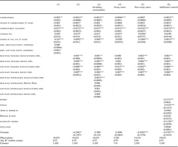
The results using the census microdata employment measures appear in Table 2. Column 1 reports the relationship between the levels of employment at manufacturing establishments that export and incumbent party presidential vote shares. We find a negative relationship between employment in low-skilled manufacturing firms that export and incumbent vote shares, and a null effect corresponding to employees of high-skilled manufacturing exports. This result is consistent with the prior findings by Feigenbaum and Hall and Margalit—exposure to competition from low-wage imports influences either Congressional roll-call votes or incumbent president vote shares, respectively.Footnote 86
County-level determinants of incumbent two-party vote shares, 1992–2012 presidential elections

Notes: The dependent variable is the change in the incumbent two-party vote share. All models include county and year fixed effects. The ten swing states are Colorado, Florida, Iowa, North Carolina, New Hampshire, Ohio, Pennsylvania, Virginia, Nevada, and Wisconsin. The trade exposure measures are log (relevant employment measure + 1) from the Census LBD. All estimates are weighted by population size in 1990. The robust standard errors (reported in parentheses) are adjusted for clustering at the county level. *p < .10; **p < .05; ***p < .01. Source: confidential plant-level employment data from the US Census Bureau.
These goods-export-employment measures are, however, unavailable for a wide range of export industries, especially in services (as noted earlier). That is, the potential winners from trade are not identified. The rest of our estimates thus rely on our measures of trade-exposed employment in manufacturing and services. We find that exposure to trade is strongly associated with presidential voting. The results in column 2 use our preferred indicators of tradability in services and manufacturing. They indicate that employment in low-wage tradable manufacturing industries is associated with lower incumbent vote shares. In contrast, employment in high-wage tradable services and high-wage tradable manufacturing is associated with higher incumbent vote shares. The estimated coefficients are statistically significant.
Substantively, a one-standard-deviation increase in (the log of) high-wage tradable manufacturing employment is associated with a 0.33 percent increase in incumbent vote share, a relatively small estimated effect. The estimates indicate substantively larger effects for low-wage manufacturing, where a one-standard-deviation change is associated with a decrease of 1.3 percent. For high- and low-wage tradable services, a one-standard-deviation change increases incumbent vote share by 1.4 percent and 1.5 percent, respectively.Footnote 87 The trade exposure variables add slightly less than 1 percent explanatory power to the county-level models.
We re-estimate the model in column 2 using the 182 LMAs as the unit.Footnote 88 The signs of the estimated coefficients are identical to the estimates using county-level data. The magnitude of the estimated coefficients is three to four times larger for the LMA models compared to the county-level models, and with the exception of high-skilled manufacturing, the coefficient estimates are statistically significant. The consistency of the result across counties and LMAs alleviates concerns about the “checkerboard” problem. (See Appendix Table A1, model 4.)
In column 3 we add four indicators of nontradable high- and low-skilled goods and services to model 2 in an effort to isolate the effects of trade from those of technological change, which would affect tradable and nontradable industries alike. The estimated effects of the indicators for the tradable sectors retain the general size, sign, and level of statistical significance. The coefficient estimates for most of the nontradable sectors are not statistically significant in this (or other) models. The exception is nontradable high-skilled manufacturing, with a positive and statistically significant coefficient.
Column 4 reports the results for swing states, which display a few notable differences from the baseline estimates. The coefficient estimate for low-wage tradable manufacturing employment is larger than the baseline model (approximately double) and statistically significant. High-wage tradable manufacturing and service employment are not statistically significant in the swing states subsample.
The results of estimates from non-swing states appear in column 5. The coefficient estimate for tradable, low-wage manufacturing employment is about a third of the size in non-swing states compared to swing states. In addition, the tradable, high-wage manufacturing and service employment measures are positively and statistically significantly associated with incumbent vote share. In column 6 we report the baseline specification plus county-level demographic controls, including education, for the full sample of counties. The coefficient estimates are quantitatively very similar to the baseline specifications.
Voter turnout is also an important electoral consideration.Footnote 89 We estimate county-level turnout models using a version of the demographic model in column 6 as the benchmark. Consistent with prior findings on turnout, we find, for example, educational attainment and race to be associated with country-level turnout.Footnote 90 Of relevance to this study, greater economic volatility is associated with higher turnout whereas concentrations of manufacturing workers is associated with lower voter turnout.Footnote 91 This is an area for future research.
In the online appendix we provide the results of a number of robustness tests designed to subject our analysis to prior findings. Table B4 demonstrates that TAA is negatively associated with incumbent vote shares, a result that confirms Margalit's finding from the 2004 presidential election.Footnote 92 Our measures of exposure to trade retain statistical significance to the inclusion of TAA, with the exception of low-wage tradable manufacturing, which loses statistical significance in the full sample but remains strongly significant in the swing states. This is not surprising, given that TAA is largely designed to address dislocations in that sector.
Our results from the county-level and labor market area analyses can be summarized as follows. Employment volatility and unemployment vary substantially across the United States, and we find strong evidence that both outcomes significantly reduce support for the incumbent. More workers in trade-exposed industries that are inconsistent with US comparative advantage (that is, tradable low-wage manufacturing) are less likely to vote for the incumbent. Increases in workers in tradable, high-wage manufacturing and tradable services are more likely to vote for the incumbent. The larger coefficient estimate for tradable, low-wage manufacturing employment and the lack of statistical significance of high-wage manufacturing and high-wage services employment in swing states might explain the persistence of policy attention to the manufacturing sector in spite of its declining share of the labor force.
Imports, Exports, and National-level US Presidential Voting
Our theory predicts that trade should have an independent, direct effect—above and beyond trade's potential indirect effects on national economic performance per se—on voting in US presidential elections. The standard approach in the national-level economic voting literature has been to estimate OLS time-series models of incumbent party presidential two-party vote shares with a necessarily limited set of explanatory variables. While investigators differ in specifications, the most commonly used approach contains measure(s) of economic performance, voter sentiment, and either prior incumbent terms or vote share. We adapt these core models and methods from the literature,Footnote 93 adding changes to the US trade balance as a variable of interest. Additional independent variables used in prior studies include retrospective indicators of economic performance: per capita real economic growth, changes in personal disposable income, job growth during a presidential term,Footnote 94 inflation during the twelve months prior to the election, and changes in unemployment. Common variables for representing voter sentiment are perceived business confidence in quarter 15 (BusSentimentQ15),Footnote 95 and presidential approval in the election-year July Gallup poll.Footnote 96 Abramowitz also incorporates how long a party has governed (duration), which captures the “costs of governing.”Footnote 97 Since we do not take a stand on the “right” macro model, we present many variants of the models with these regressors.Footnote 98
Because the list of plausible measures of the explanatory variables of Incumbent Vote Share t exceeds the plausible degrees of freedom given at most twenty observations, there is a risk of omitted variable bias in the estimations. As we noted, prior incumbent vote share (IncVoteSharet-1 ) is a plausible correlate of current vote share, and is entered to attenuate this possible bias.Footnote 99 We also estimate and report instrumental variable models using two-stage least squares (2SLS) estimators.Footnote 100
The dependent variable is the post-war incumbent party's share of the two main party presidential votes (incumbent 2-party vote share t ) from 1952 to 2012. The sample is determined by the availability of quarterly data on economic growth.Footnote 101 In most of our models, the investigation starts with the 1952 data. We also estimate a model, 1936–2012, using data from Fair.Footnote 102 The passage of the Reciprocal Trade Agreements Act (RTAA) of 1934 repealed the Smoot-Hawley Tariff, and is widely seen as marking the modern era of US trade integration.Footnote 103
In light of prior theory and statistical modeling, our base time-series OLS macro model is:
 $$\eqalign{& Incumbent\,Two-Party\,Vote\,Share_t = {\beta}_0 + {\beta}_{1} \left( {Incumbent\,Vote\,Share_{t - 1}} \right) \cr & \quad + {\beta}_2 \left( {Economic\,Growth_{t - 1}} \right)\; + \varepsilon _t \ t = 1952-2012} $$
To this model will be added change in the trade indicators:
either ß3(ΔTradeBal/GDPt-1) or ß3′(ΔImport/GDPt-1) and ß4′(ΔExports/GDPt-1), plus an indicator of either Business Sentiment or July Approval: ß5(Sentiment/Approval t-1). A model that replaces prior incumbent vote share with prior incumbent terms (duration) is also reported.Footnote 104 The timing of the variables is such that monthly data (when available) after the presidential elections in November are excluded.
To assess the statistical adequacy of the OLS time-series models, a number of descriptive statistics, diagnostic tests, correlations, and factor analyses are reported. These can be found in the online appendix. The statistical adequacy of the model is especially important in the context of a small number of observations with potentially correlated errors.Footnote 105
National-level Election Results
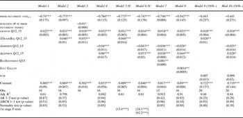
Table 3 reports the main results. In column 1, prior incumbent vote share and economic growth are entered. The estimation properties of the model are good, and the results are consistent with prior findings. Importantly, economic growth has an estimated coefficient that is positive, significant, and substantively large. The lagged endogenous variable has a negative and significant coefficient, which is consistent with the theories regarding the “costs of governing” and the standard findings of a decline in incumbent vote margins in subsequent elections.
Base models—dependent variable is national incumbent party (two-party) vote shares (1952–2012, 1936–2012)

Notes: The standard errors are generally heteroskedasticity and autocorrelation consistent standard errors. Model 3 reports a Prais-Winsten AR1 regression (ρ=−.41). The standard errors for the IV models (5 and 6) are robust standard errors corrected for small sample bias. The IV Adj. R2 is the Generalized Adj. R2 from Pesaran and Smith Reference Pesaran and Smith1994 for IV models. Data for the 1936, 1940, 1944, and 1948 elections are from Fair Reference Fair2009 and the BEA. *p < .10; **p < .05; ***p < .01.
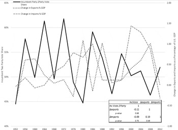
In column 2, change in the trade balance enters with a statistically significant positive coefficient that is substantively large and consistent with the theory we developed. A one-unit increase (decrease) in the US trade balance as a percentage of GDP is associated with a 4 percent estimated increase (decrease) in incumbent vote shares.Footnote 106 Column 3 substitutes prior incumbent terms from the Abramowitz “time for change” modelFootnote 107 for incumbent vote shares: a one-unit increase (decrease) in the US trade balance as a percentage of GDP is associated with a 3 percent estimated increase (decrease) in incumbent vote shares. Change in imports (column 4) has a statistically significant negative coefficient, which is substantively large and also consistent with our theory. A one-unit increase (decrease) in imports as a percentage of GDP is associated with a 4 percent decrease (increase) in incumbent vote shares. Change in exports as a percentage of GDP has a positive and statistically significant coefficient that is substantively large; a one-unit increase is associated with a 6 percent increase in presidential vote shares. The explanatory power of the models, judged via adjusted R-squared indicators, rises nineteen points with the inclusion of the trade variables.Footnote 108
Columns 5 and 6 report the 2SLS models (described earlier). The estimated coefficients for the trade variables are similar in size, sign, and level of statistical significance to their OLS counterparts. The levels of statistical significance of the models (given as the generalized adjusted R2 for instrumental variable (IV) models from Pesaran and Smith)Footnote 109 are similar to their OLS counterparts.
In columns 7 and 8, using ΔImport/GDPt-1 and ΔExports/GDPt-1 , we add business sentiment Q15 and July Gallup, respectively. The models have good estimation properties and explanatory power. Both business sentiment Q15 and July Gallup have positive, statistically significant, and substantively large estimated coefficients that are consistent with prior theory and findings.Footnote 110 The estimated coefficient of ΔImport/GDPt-1 remains negative and highly statistically significant, and the estimated coefficient of ΔExport/GDPt-1 remains positive and statistically significant.Footnote 111 As a further test, we extend the sample back to the 1936 election, which is post-RTAA, using data and models from Fair.Footnote 112 Column 9 enters changes in the trade balance, and column 10 enters changes in imports and exports. The coefficient estimates retain similar signs and levels of statistical significance.
In the online appendix (Table B5), we use model 3.4 as the base model and add additional indicators proposed by other investigators, including changes in multifactor productivity to measure technological innovation, changes in the unemployment rate, changes in inflation, and a time trend.Footnote 113 The magnitudes, directions, and statistical significances of the trade results are strongly robust to including these other regressors. In all cases, the export and import coefficient estimates retain the expected sign, and the estimated coefficients are statistically significant at the 0.05 level or better.Footnote 114
Conclusion
Prior academic research indicates that globalization—characterized by increases in financial integration, rising exports and import competition, and the offshoring of production—shapes politics through its effects on employment, wages, and economic insecurity. We demonstrate that changes in trade flows and changes in employment in firms in winning and losing service and manufacturing industries influence presidential voting.
Rising employment in high-skilled service exports—which captures trade's expected winners in the US—is associated with increasing incumbent vote shares. Rising employment in high-skilled tradable manufacturing is also associated with increasing incumbent vote shares, although the magnitude of the estimated effects is much smaller than for high-skilled tradable services. In line with other studies, we find strong evidence that the concentration of economic activity in low-skilled tradable manufacturing diminishes incumbent vote shares. At the national level, using established models and IV estimations, we report the novel finding that rising exports (imports) are associated with rising (declining) incumbent vote shares.
We find some evidence that Electoral College considerations provide an incentive against the further liberalization of trade. The estimated negative effects of low-skilled manufacturing are largely found in the swing states. In contrast, the estimated effects of rising employment in both high-skilled services and high-skilled manufacturing are found only in non-swing states. The extent, therefore, to which the contestability of employment and economic insecurity from trade, rather than purely domestic economic concerns, shapes presidential election outcomes suggests a necessary coupling of previously isolated research streams in American politics and international political economy.
Our results also offer a contrast to recent findings regarding sociotropic theories of trade wherein the distributional consequences of trade per se have little to do with voter attitudes toward trade. While our work does not explicitly examine voter attitudes, we find a very robust correlation between objective economics of trade indicators and citizen voting behavior at the county and labor market areas. Voters appear to be acting as if they were responding to the trade exposure of their geographic region.
Supplementary Material
Supplementary material for this article is available at <https://doi.org/10.1017/S0020818317000194>.
Appendix A
Correlation between education and salary

Time series of the dependent and key independent trade variables

Varying tradability cut-offs and labor market area results