1 Introduction
In recent years, researchers have identified numerous electron scale plasma instabilities (Weibel Reference Weibel1959; Bret, Firpo & Deutsch Reference Bret, Firpo and Deutsch2004; Gruzinov Reference Gruzinov2008; Alves et al. Reference Alves, Grismayer, Fonseca and Silva2015) that are thought to be important in astrophysical and laboratory phenomena (Fiuza et al. Reference Fiuza2012; Stockem et al. Reference Stockem2014), including shocks (Gregori et al. Reference Gregori2012), particle acceleration (Gruzinov & Waxman Reference Gruzinov and Waxman1999; Medvedev & Loeb Reference Medvedev and Loeb1999) and magnetogenesis (Kulsrud & Zweibel Reference Kulsrud and Zweibel2008; Alves et al. Reference Alves, Grismayer, Martins, Fiuza, Fonseca and Silva2012; Grismayer et al. Reference Grismayer, Alves, Fonseca and Silva2013; Nishikawa et al. Reference Nishikawa2013; Alves et al. Reference Alves, Grismayer, Fonseca and Silva2014; Miller & Rogers Reference Miller and Rogers2015). The electron scale Kelvin–Helmholtz instability (ESKHI) is one example. Classically, the KHI is a neutral fluid phenomenon driven by velocity shear (Biskamp Reference Biskamp2003). The mode in its simplest form requires subsonic bulk velocity, and is strongest for wave vectors  $k\sim 1/L$ parallel to the flow, where
 $L$ is a typical gradient scale length of the flow profile. The ESKHI, which occurs in plasmas with sharp (electron scale) flow variations, is a related electromagnetic mode at higher frequencies and smaller scales (i.e. scale sizes comparable to the electron skin depth
 $d_{e}\equiv c/{\it\omega}_{pe}$). Recently, Gruzinov (Reference Gruzinov2008) demonstrated that in the relativistic regime, there exists a second mechanism for shear-driven instability. This instability is electromagnetic, and operates at wavelengths longer than
 $d_{e}$, albeit with low growth rates when the shear velocity
 $V_{0}$ is small compared to the speed of light
 $c$. Very recently, Alves et al. (Reference Alves, Grismayer, Martins, Fiuza, Fonseca and Silva2012, Reference Alves, Grismayer, Fonseca and Silva2015), Grismayer et al. (Reference Grismayer, Alves, Fonseca and Silva2013) have explored similar instabilities with wave vectors transverse to the flow. The bulk of this previous work has assumed a cold plasma,
 $T_{i}=T_{e}=0$. In the typical Kelvin–Helmholtz (KH) case of waves propagating parallel to the flow, we expand this effort to include finite temperatures, utilizing the relativistic fluid framework of Synge (Reference Synge1957, equations (B1)); this permits relativistically high temperatures
 $(T_{i},T_{e}>m_{i}c^{2},m_{e}c^{2})$. We find that quite generally, the addition of finite temperature is destabilizing. This is demonstrated for two simple cases; free-streaming ions (i.e.
 $V_{i}=V_{0}$ or equivalently
 $m_{i}\rightarrow \infty$) and equal thermal speeds (
 $V_{ti}=V_{te}$, relevant to the ultra-hot case or the case of electron–positron plasmas). With either constraint, unstable, purely growing modes (i.e. positive real roots to the dispersion relation) occur in two neighbouring parameter regimes, associated with Gruzinov’s instability and the ESKHI. Outside these regions, the coupling of the modes produces residual instability; all wavenumbers in this domain are unstable, with maximum growth rates occurring for wavelengths near the electron skin depth
 $(k^{-1}\approx d_{e})$. Consequently, the system is unstable for any finite temperature. Because we utilize a fluid model, the applicability of this theory to collisionless plasmas is problem dependant. In such a system, these results should be interpreted with caution. That said, most of the existing studies on this topic use a kinetic approach (Bret et al. Reference Bret, Firpo and Deutsch2004; Alves et al. Reference Alves, Grismayer, Martins, Fiuza, Fonseca and Silva2012, Reference Alves, Grismayer, Fonseca and Silva2015; Grismayer et al. Reference Grismayer, Alves, Fonseca and Silva2013); here we present a fluid treatment, which derives many of the same results.
Before continuing, we must clarify an ambiguity in the terminology. Two completely distinct effects are commonly referred to as the Kelvin–Helmholtz instability (KHI). Traditionally, the KHI is an acoustic phenomenon found in neutral fluids. This is the instability presented in most introductory texts (Biskamp Reference Biskamp2003). It requires subsonic sheared velocity  $(V_{0}<V_{t})$ to operate, often implicitly assumed by using the incompressible equations. Gruzinov (Reference Gruzinov2008) and Alves et al. (Reference Alves, Grismayer, Fonseca and Silva2015), on the other hand, use an electromagnetic analogue to the KHI. Gruzinov calls this effect (Gruzinov Reference Gruzinov2008) the ‘relativistic collisionless Kelvin–Helmholtz instability’. Alves et al. (Reference Alves, Grismayer, Fonseca and Silva2015) refer to it as the electron scale Kelvin–Helmholtz instability (ESKHI). However, as both Alves et al. and Gruzinov assume
 $T=0$ (or at least
 $V_{t}\ll V_{0}$), the physics of the effects they describe are fundamentally distinct from traditional KHI dynamics. Henceforth, we refer to their mode as the ‘relativistic electron scale shear instability’ (RESI). The term ESKHI is reserved for the electron scale, sub-thermal speed mode that was absent in Gruzinov’s
 $T=0$ work, i.e. the dispersion relation that, in the subsonic, non-relativistic, neutral limit, recovers the traditional KHI dispersion relation found in introductory texts (Biskamp Reference Biskamp2003). Finally, note that the dynamics of both modes are distinct from effects arising in the context of standard electron magnetohydrodynamics with motionless ions, including the instability frequently referred to as the electron Kelvin–Helmholtz instability.
2 Description of instabilities
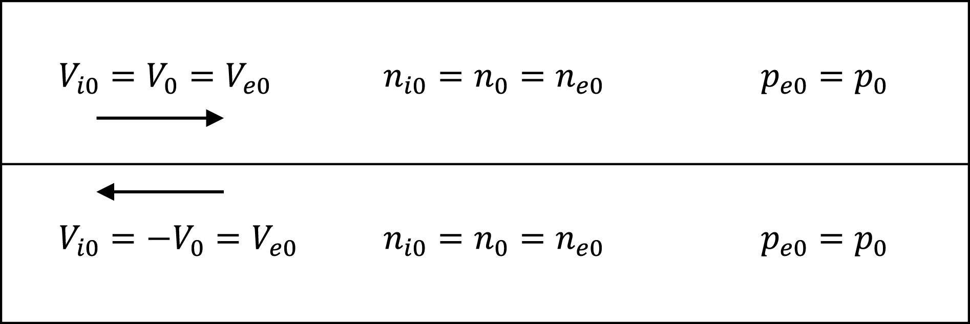
Consider a collisionless ion–electron plasma with discontinuous sheared flow in the centre-of-momentum frame (figure 1). The bulk velocity of ions and electrons is  $V_{0}\hat{\boldsymbol{y}}$ above the discontinuity and
 $-V_{0}\hat{\boldsymbol{y}}$ below (these regimes are indicated by subscripts
 $a$ and
 $b$ where appropriate). Following Gruzinov (Reference Gruzinov2008), we are analysing waves propagating in the
 $y$-direction, parallel to the flow. The unperturbed plasma is assumed to be unmagnetized, charge neutral and current free, with uniform density and pressures.
The Kelvin–Helmholtz shear discontinuity system.

Assuming free-streaming ions  $(m_{i}=\infty )$ linear perturbations with wavenumber
 $k$ along the discontinuity and growth rate
 ${\it\lambda}$ satisfy a dispersion relation in terms of electron plasma frequency
 ${\it\omega}_{e}$ and thermal speed
 $V_{te}$ (see appendix A for a discussion of the relativistic parameters). Normalizing velocities to the speed of light
 $c$, frequencies to the electron plasma frequency over the Lorentz factor
 ${\it\gamma}_{0}=(1-V_{0}^{2})^{-1/2}$ and wavenumbers to the skin depth over
 ${\it\gamma}_{0}$ (B 10a–d), this dispersion relation is (a derivation of (2.1) is outlined in appendix B. A far more general equation including three dimensions and ion motion can be found in the supplementary materials available online at http://dx.doi.org/10.1017/S0022377816000180. This general equation encompasses the RESI, ESKHI and transverse mushroom instability found by Alves et al. (Reference Alves, Grismayer, Fonseca and Silva2015))
 $$\begin{eqnarray}\displaystyle 0=S({\it\lambda})\equiv RFG-2V_{0}^{2}V_{te}{\it\lambda}^{2}D^{2}, & & \displaystyle\end{eqnarray}$$
where
 $$\begin{eqnarray}\displaystyle & \displaystyle F\equiv ({\it\lambda}^{2}+V_{0}^{2}k^{2})^{2}+{\it\lambda}^{2}-V_{0}^{2}k^{2}, & \displaystyle\end{eqnarray}$$
 $$\begin{eqnarray}\displaystyle & \displaystyle D\equiv 1+2k^{2}+{\it\lambda}^{2}-V_{0}^{2}k^{2}, & \displaystyle\end{eqnarray}$$
 $$\begin{eqnarray}\displaystyle & \displaystyle G\equiv (1+({\it\lambda}-\text{i}kV_{0})^{2})W_{a}+(1+({\it\lambda}+\text{i}kV_{0})^{2})W_{b}, & \displaystyle\end{eqnarray}$$
 $$\begin{eqnarray}\displaystyle & \displaystyle R\equiv \sqrt{1+\frac{k^{2}}{{\it\gamma}_{0}^{2}}+\frac{{\it\lambda}^{2}}{{\it\gamma}_{0}^{2}}}, & \displaystyle\end{eqnarray}$$
 $$\begin{eqnarray}\displaystyle & \displaystyle \text{and}\quad W_{a/b}\equiv \sqrt{1+({\it\lambda}\pm \text{i}kV_{0})^{2}-(\pm {\it\lambda}V_{0}+\text{i}k)^{2}V_{te}^{2}}. & \displaystyle\end{eqnarray}$$
Assuming equal thermal speeds  $(V_{ti}=V_{te})$ instead of free-streaming ions leads to an identical equation (upon substituting
 ${\it\omega}_{p}^{2}={\it\omega}_{e}^{2}+{\it\omega}_{i}^{2}$ for
 ${\it\omega}_{e}^{2}$); this is relevant to the ultra-hot limit, since as
 $T\rightarrow \infty$ thermal velocities cannot exceed
 $c/\sqrt{3}$ (see appendix A), or to an electron–positron plasma (assuming
 $T_{e}=T_{p}$). As shown in appendix B,
 $W$ and
 $R$ are the inverse decay lengths of the acoustic and light wave modes, respectively. The dispersion relation
 $F=0$ is the RESI, with solutions (Gruzinov Reference Gruzinov2008):
 $$\begin{eqnarray}\displaystyle {\it\lambda}^{2}={\textstyle \frac{1}{2}}\left(-1-2V_{0}^{2}k^{2}\pm \sqrt{1+8V_{0}^{2}k^{2}}\right). & & \displaystyle\end{eqnarray}$$
 $R=0$ gives a plasma light wave with frequency
 ${\it\lambda}^{2}=-k^{2}-{\it\gamma}_{0}^{2}$, and
 $G=0$ results in the electron acoustic mode/ESKHI, with roots given by a subset of
 $$\begin{eqnarray}\displaystyle & \displaystyle {\it\lambda}^{2}=0_{+},\quad \frac{1}{1+V_{te}^{2}-2V_{0}^{2}V_{te}^{2}}\left(\vphantom{\sqrt{\left(\frac{k^{2}}{{\it\gamma}_{0}^{4}}-V_{0}^{2}\right)^{2}}}-1-k^{2}V_{0}^{2}-V_{te}^{2}\left(\frac{k^{2}}{{\it\gamma}_{0}^{4}}-V_{0}^{2}+1-k^{2}V_{0}^{2}\right)\right. & \displaystyle \nonumber\\ \displaystyle & \displaystyle \hspace{40.00006pt}\left.\pm \,\sqrt{4k^{2}V_{0}^{2}+4k^{2}V_{0}^{2}\left(\frac{k^{2}}{{\it\gamma}_{0}^{4}}-V_{0}^{2}\right)V_{te}^{2}+\left(\frac{k^{2}}{{\it\gamma}_{0}^{4}}-V_{0}^{2}\right)^{2}V_{te}^{4}}\right). & \displaystyle\end{eqnarray}$$
For these three fundamental modes, the roots are either purely real (growing/decaying) or purely imaginary (oscillatory). It is straightforward to derive their regimes of instability; the RESI has unstable solutions in the range  $0<k^{2}V_{0}^{2}<1$ (Gruzinov Reference Gruzinov2008) and the ESKHI is unstable when
 $$\begin{eqnarray}\displaystyle 1<k^{2}V_{0}^{2}<1+V_{te}^{2}k^{2}\frac{2}{(1+V_{te}^{2})}. & & \displaystyle\end{eqnarray}$$
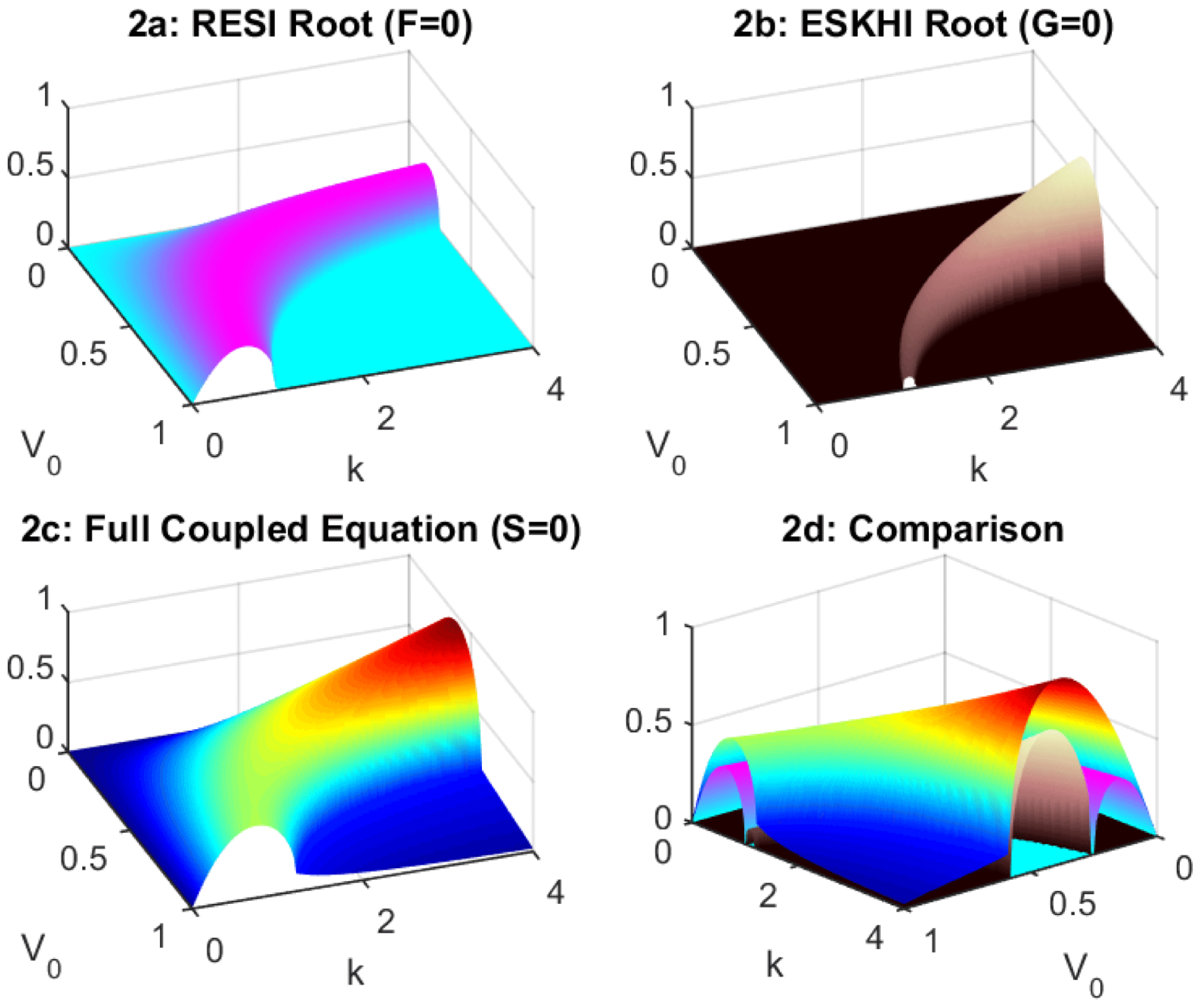
The growth rate of the most unstable roots as a function of  $V_{0}$ and
 $k$, at
 $V_{te}=0.4$.

The light wave mode is always stable. The second term in (2.1) provides a coupling between these modes. This coupling amplifies the existing purely real instabilities, while generating smaller, complex instabilities in previously stable parameter regimes.
Figure 2 highlights the relationships between roots of  $F=0$,
 $G=0$ and
 $S=0$. The surfaces show the maximum real part of
 ${\it\lambda}$, as a function of bulk velocity
 $V_{0}$ and wavenumber
 $k$, at a thermal speed
 $V_{te}=0.4$. Figures 2(a) and 2(b) present the real portions of (2.3) and (2.4), respectively. The unstable regions of both functions are bounded by limits given above, meeting as predicted where
 $kV_{0}=1$. Outside of these boundaries, growth rates are purely imaginary. Figure 2(c) shows the real components of numerical roots for (2.1) at the same temperature. The coupling increases the growth rate of existing instabilities and merges the regimes of figures 2(a) and 2(b). Between the ESKHI cutoff (2.5) and
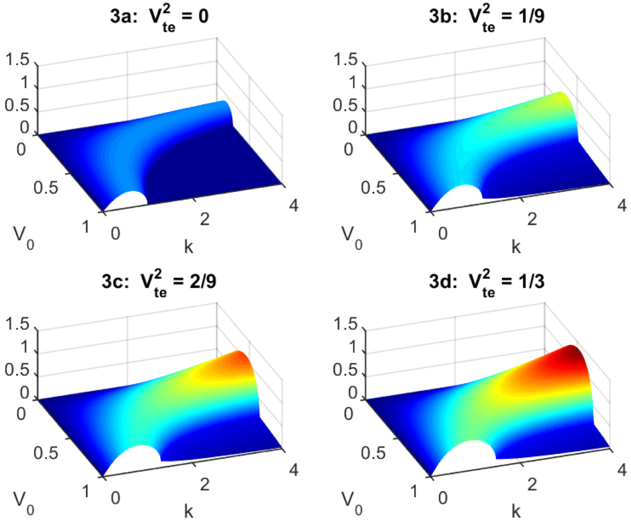
 $kV_{0}=0$, modes have highly unstable, purely real roots. In the region beyond this cutoff, residual coupling of the instabilities creates smaller, complex roots. In figure 2(d), the previous three plots are superimposed. This more clearly demonstrates that regions unstable to RESI or ESKHI independently are even less stable in the fully coupled equation. Furthermore, outside these bounds, lingering instability remains. Figure 3 presents numerical solution to (2.1) at various temperatures. As temperature increases, instability (in normalized units) increases everywhere. The regime of large instability also stretches along both axes, as suggested by (2.5).
The growth rate of the most unstable roots of equation (2.1)  $(S=0)$ as a function of
 $V_{0}$ and
 $k$ for various
 $V_{te}$.

Before discussing the complex roots in depth, we prove that the highly unstable roots are purely real, and that the bound on the region of high instability closely matches the bound on ESKHI given in (2.5). The function  $S({\it\lambda})$ is holomorphic everywhere that
 $Re({\it\lambda})\neq 0$ (a sufficient but not necessary condition). Thus for all non-zero real
 ${\it\lambda}$,
 $S({\it\lambda})$ is real. As
 ${\it\lambda}$ goes to real infinity,
 $S({\it\lambda})$ grows to positive infinity as well (the leading term proportional to
 ${\it\lambda}^{8}$ is positive). Therefore, if
 $S({\it\lambda})$ is negative for small
 ${\it\lambda}$, there must exist some positive real value which satisfies
 $S({\it\lambda})=0$, i.e. there must exist a purely growing unstable mode. Taylor expanding (2.1), a positive real root is guaranteed when
 $$\begin{eqnarray}\displaystyle k^{2}V_{0}^{2}\leqslant 1+V_{te}^{2}k^{2}\frac{2}{(1+V_{te}^{2})}. & & \displaystyle\end{eqnarray}$$
Thus the upper bound on the domain of real roots for ESKHI (2.5) is also a sufficient condition for a real root to the fully coupled equation  $S({\it\lambda})$. Numerical modelling shows that this closely matches the necessary condition as well; only in a narrow parameter regime is
 $S({\it\lambda})$ positive for
 ${\it\lambda}\ll 1$ and negative at some finite
 ${\it\lambda}$ (thus generating a pair of roots; these narrow regions appear in figures 4 and 5). It can also be noted that there is exactly one positive real root when (2.6) is met, and that when
 $k^{2}V_{0}^{2}<1+V_{te}^{2}k^{2}$ the root at
 ${\it\lambda}=0_{+}$ vanishes as well.
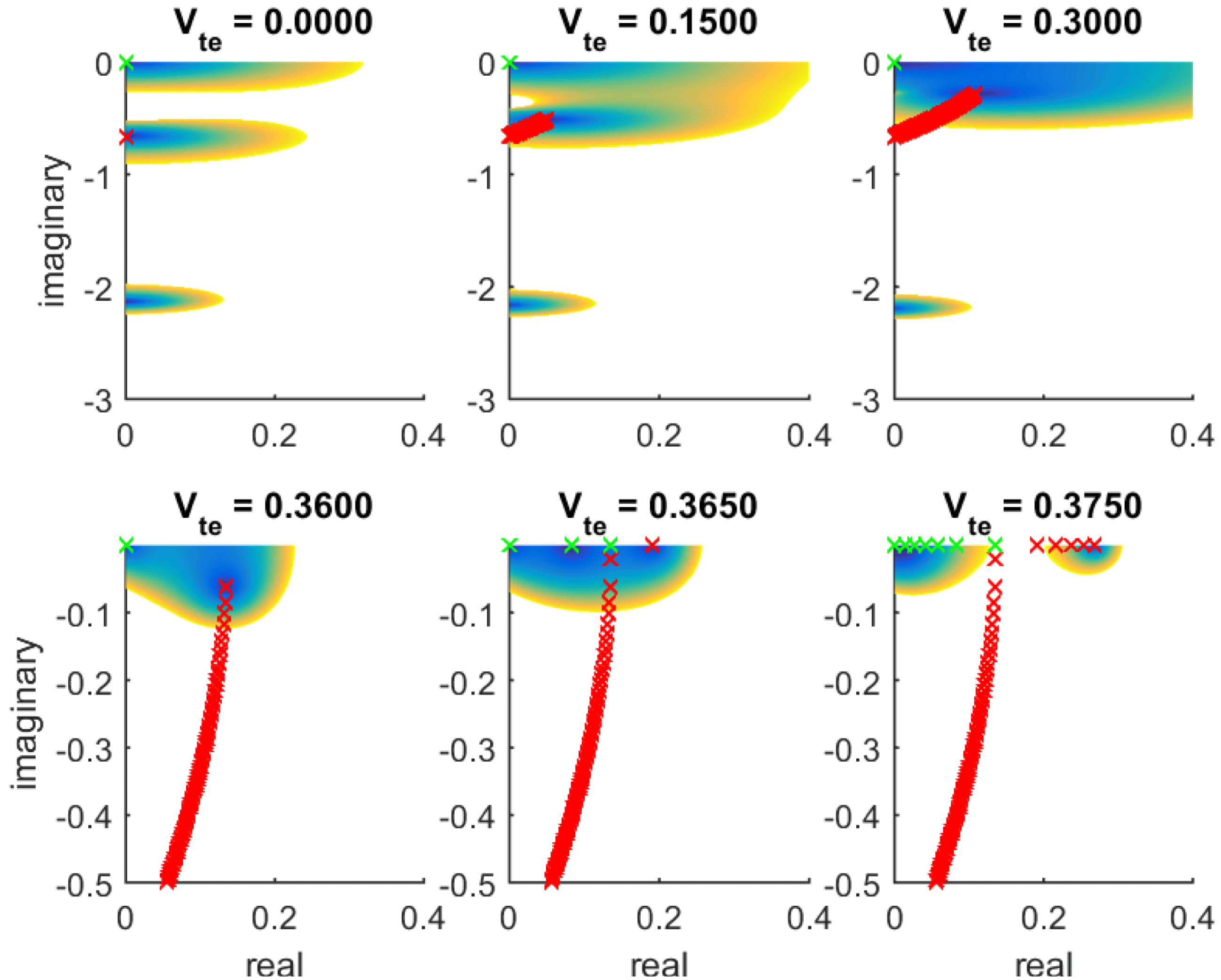
The absolute value of  $S({\it\lambda}_{real}+\text{i}{\it\lambda}_{imag})$, using
 $V_{0}^{2}=1/2$,
 $k=2$, and increasing values of
 $V_{te}$ ‘
 $\times$’ marks indicate the path of the roots as
 $V_{te}$ increases from zero in steps of
 ${\rm\Delta}V_{te}=0.0025$ For the top three images, the colour scales go from 0 (blue) to 3 (red). In the bottom three, the max cutoff is 0.1. Videos of this motion are available online.

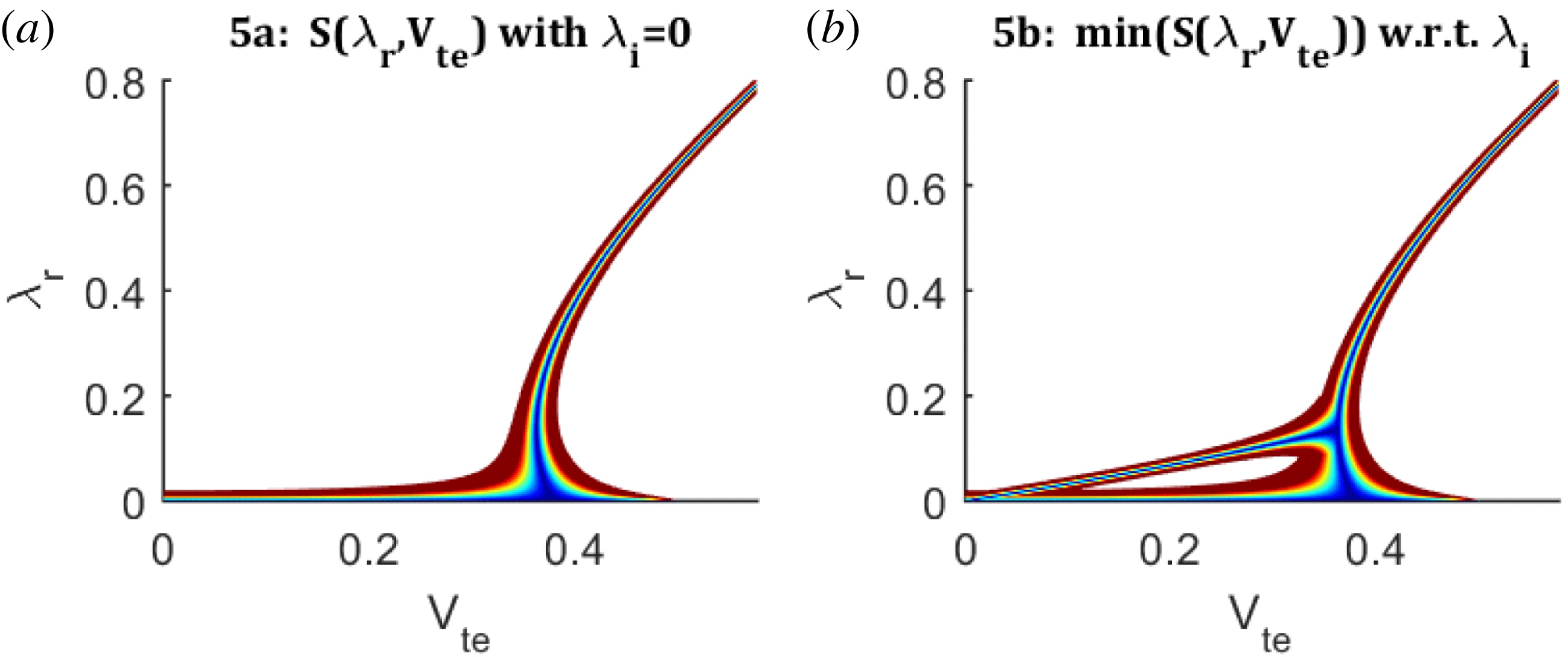
The absolute value of  $S({\it\lambda}_{real},V_{te})$, using
 $V_{0}^{2}=1/2$,
 $k=2$. (a) assumes
 ${\it\lambda}_{imag}=0$. In (b), the minimum of
 $S({\it\lambda}_{real},V_{te})$ with respect to
 ${\it\lambda}_{imag}$ is presented.

Figures 4 and 5 illustrate the progression of the roots of  $S({\it\lambda})$ as
 $V_{te}$ increases. Both figures plot the absolute value of the function
 $S({\it\lambda}_{real}+\text{i}{\it\lambda}_{imag},V_{te})$, for
 $V_{0}^{2}=1/2$,
 $k=2$. Thus, roots exist where the surfaces hit zero (deep blue). Note that to remove spurious roots, the actual function being plotted is
 $S/((({\it\lambda}+\text{i}kV_{0})^{2}+1)(({\it\lambda}-\text{i}kV_{0})^{2}+1))$. Figure 4 shows the
 ${\it\lambda}_{real}{-}{\it\lambda}_{imag}$ plane, at various
 $V_{te}$ slices (while only the fourth quadrant is presented,
 $S({\it\lambda})$ is symmetric across both axes). A video version of this figure, which is perhaps more illuminating, can be found in the supplementary movie online. At
 $V_{te}=0$, the roots are the purely imaginary solutions to
 $R=0,F=0$ and
 $G=0$. Once finite temperature is included, the coupling term in (2.1) interferes. The positive RESI root (tracked by red ‘
 $\times$’ marks) drifts off the imaginary axis. The ESKHI root at
 ${\it\lambda}=0_{+}$ remains (green
 $\times$), but the negative RESI root ceases to be a true zero of the equation, as does the light wave root. As
 $V_{te}$ increases, the real component of what used to be the positive RESI root continues to increase and the imaginary component decreases. Isolating the thermal velocity in (2.6) results in
 $$\begin{eqnarray}\displaystyle V_{te}^{2}<\frac{k^{2}V_{0}^{2}-1}{1+2k^{2}-k^{2}V_{0}^{2}}. & & \displaystyle\end{eqnarray}$$
Just prior to exceeding this condition, the root becomes purely real. The two roots on either side of the real axis merge and redivide into two roots along the real axis. One of these roots drops towards zero (marked in green), and the other increase rapidly with  $V_{te}$. When the two sides of (2.7) are exactly equal, the falling root reaches zero and merges with the
 ${\it\lambda}=0_{+}$ root (
 ${\it\lambda}=0$ itself is not a root unless very specific parameters are chosen). For temperatures higher than this, there is only a single positive real root to the equation. Finally, when
 $k^{2}V_{te}^{2}=k^{2}V_{0}^{2}-1$,
 ${\it\lambda}=0_{+}$ ceases to be a root as well. Figure 5 shows the same behaviour from the
 ${\it\lambda}_{real}{-}V_{te}$ plane. In figure 5(a),
 ${\it\lambda}_{imag}$ is set to zero. In figure 5(b), the value plotted is the minimum of
 $S({\it\lambda}_{real},V_{te})$ across all
 ${\it\lambda}_{imag}$. The behaviour matches the above description. For low
 $V_{te}$, only complex roots and the root at
 ${\it\lambda}=0_{+}$ exist. The instability grows with
 $V_{te}$, and just before the threshold of (2.7) is reached, the roots become purely real. There are briefly two positive real roots, one growing with
 $V_{te}$ and one shrinking, the latter reaching zero when (2.7) is satisfied.
Before concluding, we will briefly comment on the connection between this work and the paper recently published by Alves et al. (Reference Alves, Grismayer, Fonseca and Silva2015). It is verified that for high  $V_{0}$ and low
 $V_{te}$, there exists a
 $k$ which maximizes growth rate (seen in (2.6) and figure 3). However, setting
 $k$ to infinity in (2.6) results in the condition
 $$\begin{eqnarray}\displaystyle V_{0}^{2}\leqslant V_{te}^{2}\frac{2}{(1+V_{te}^{2})}. & & \displaystyle\end{eqnarray}$$
If (2.8) is satisfied, the system remains highly unstable for all wavenumbers and the growth rate increases as  $k$ goes to infinity. In the ultra-hot case
 $V_{te}^{2}\rightarrow 1/3$, (2.8) reads
 $V_{0}^{2}\leqslant 1/2$. Of course, this is assuming a discontinuity in the velocity profile; given a smoother shear with gradient scale length
 $L$, a maximizing wavelength will likely be found with
 $k\sim L^{-1}$ (Grismayer et al. Reference Grismayer, Alves, Fonseca and Silva2013; Alves et al. Reference Alves, Grismayer, Fonseca and Silva2014).
We also confirm the ‘mushroom’ instability described by Alves et al. (Reference Alves, Grismayer, Fonseca and Silva2015). Considering the transverse  $x$–
 $z$ plane instead of the parallel
 $x$–
 $y$ plane, the dispersion relation
 $$\begin{eqnarray}\displaystyle 0=({\it\lambda}^{2}({\it\lambda}^{2}+1)+k_{z}^{2}({\it\lambda}^{2}-{\it\gamma}_{0}^{2}V_{0}^{2}))\left(-\left(\frac{{\it\lambda}^{2}}{{\it\gamma}_{0}^{2}}+1\right)W^{\prime }+V_{0}^{2}V_{t}R^{\prime }\right) & & \displaystyle\end{eqnarray}$$
is reached (see the general 3-D equation presented in the supplementary material), where
 $$\begin{eqnarray}\displaystyle W^{\prime }=\sqrt{({\it\lambda}^{2}+1)-\left({\it\lambda}^{2}V_{0}^{2}-\frac{1}{{\it\gamma}_{0}^{2}}k_{z}^{2}\right)V_{te}^{2}},\quad R^{\prime }=\sqrt{\frac{{\it\lambda}^{2}}{{\it\gamma}_{0}^{2}}+\frac{k_{z}^{2}}{{\it\gamma}_{0}^{2}}+1}. & & \displaystyle\end{eqnarray}$$
The roots arising from the first factor are equivalent to (2.1) in Alves et al. (Reference Alves, Grismayer, Fonseca and Silva2015). The roots arising from the second factor are stable for all values of  $V_{0},k_{z}$ and
 $V_{te}$. In general, parallel modes grow faster in the highly unstable regimes discussed above, and perpendicular modes grow more rapidly elsewhere. This connection demonstrates that in the discontinuity regime under consideration, the simple fluid model presented here derives the same results as the kinetic approach established by other researchers.
3 Conclusion
We have shown that upon including temperature, parallel wave perturbations to relativistic shear flows are ubiquitously unstable at small scales. Strong instability (growth rates of order  ${\it\omega}_{p}$) occur in both the relativistic regime highlighted by Gruzinov (Reference Gruzinov2008) and the standard ESKHI region; with free-flowing ions (or equal ion and electron thermal speeds), the condition for large instability is expressed in (2.6),
 $$\begin{eqnarray}\displaystyle k^{2}V_{0}^{2}\leqslant 1+V_{te}^{2}k^{2}\frac{2}{(1+V_{te}^{2})}. & & \displaystyle\end{eqnarray}$$
When this condition is met, we have found that growth rates are substantially larger in warm plasmas than in the  $T=0$ plasmas studied previously (Weibel Reference Weibel1959; Gruzinov Reference Gruzinov2008; Alves et al. Reference Alves, Grismayer, Martins, Fiuza, Fonseca and Silva2012, Reference Alves, Grismayer, Fonseca and Silva2015) (up to triple for large temperatures); this parallels the findings of Grismayer’s kinetic simulations (Grismayer et al. Reference Grismayer, Alves, Fonseca and Silva2013). Even when velocity exceeds condition (3.1), a smaller, complex instability remains. In order to eliminate instability completely, it is necessary to eliminate the coupling term in (2.1). This requires setting either
 $V_{0}=0$ (i.e. no shear) or
 $T=0$ (cold plasma). As demonstrated in appendix B, the coupling term arises from the electromagnetic response to electron acoustic motion. When (2.8) is met, the growth rate appears to increase indefinitely with wavenumber. Otherwise, a fastest growing mode exists with wavelength near the electron skin depth. In a more physical scenario with smoother velocity gradient, presumably as in similar systems, the maximum growth rate is limited by the scale size of the shear (Grismayer et al. Reference Grismayer, Alves, Fonseca and Silva2013; Alves et al. Reference Alves, Grismayer, Fonseca and Silva2014). Finally, it is unlikely that the saturation condition of these modes will be substantially different than for the cold plasmas already studied. These instabilities saturate when the DC magnetic field they generate grows strong enough to arrest the flow of electrons across the field. Grismayer et al. estimate that this occurs around (Grismayer et al. Reference Grismayer, Alves, Fonseca and Silva2013)
 $$\begin{eqnarray}\displaystyle B=\frac{m_{e}{\it\omega}_{e}}{q}V_{0}\sqrt{{\it\gamma}}_{0}. & & \displaystyle\end{eqnarray}$$
For magnetogenesis applications, it is the growth of this field itself which is most important.
Supplementary material
Supplementary material is available at http://dx.doi.org/10.1017/S0022377816000180.
Appendix A. A note on relativistic variables
The relativistic analogues of the electron plasma frequency and electron thermal speed satisfy
 $$\begin{eqnarray}\displaystyle {\it\omega}_{e}^{2}\equiv \frac{q^{2}n_{0}}{{\it\varepsilon}_{0}m_{e}f_{e}{\it\gamma}_{0}^{2}},\quad \frac{V_{te}^{2}}{c^{2}}=\frac{\displaystyle \frac{z_{e}}{f_{e}}\frac{\text{d}f_{e}}{\text{d}z_{e}}}{\displaystyle z_{e}^{2}\frac{\text{d}f_{e}}{\text{d}z_{e}}+1},\quad \text{where }z_{e}=\frac{m_{e}c^{2}}{T_{e}},\;f_{e}=\frac{K_{3}(z_{e})}{K_{2}(z_{e})}. & & \displaystyle\end{eqnarray}$$
The factor  $f_{e}$, a ratio of two modified Bessel functions of the second kind, is the relativistic correction to mass due to thermal motion (similar to the Lorentz correction
 ${\it\gamma}$ for linear motion). For a detailed analysis of this term and derivation of the thermal velocity, see Synge (Reference Synge1957). Importantly, for low temperatures, the classical result
 $V_{t}^{2}=5T/3m$ is recovered, while at high temperatures, a maximum
 $V_{t}$ is reached,
 $$\begin{eqnarray}\displaystyle \lim _{T\rightarrow \infty }\frac{V_{t}^{2}}{c^{2}}=\frac{1}{3}. & & \displaystyle\end{eqnarray}$$
This is analogous to how the Lorentz factor  ${\it\gamma}$ prevents a particle’s linear velocity from exceeding
 $c$, regardless of how much kinetic energy it possesses.
Appendix B. Derivation of instability
Following the work of Synge (Reference Synge1957) and Mahajan (Reference Mahajan2003), the equations for a relativistic plasma are found by integrating Vlasov equation assuming a Maxwell–Juttner distribution. They consist of species-specific continuity equations
 $$\begin{eqnarray}\displaystyle \partial _{{\it\mu}}n_{o}U^{{\it\mu}}=0, & & \displaystyle\end{eqnarray}$$
species-specific equations of motion
 $$\begin{eqnarray}\displaystyle -\partial ^{{\it\nu}}(n_{o}T)+mn_{o}U^{{\it\mu}}\partial _{{\it\mu}}(fU^{{\it\nu}})=qn_{o}U_{{\it\mu}}\unicode[STIX]{x1D60D}^{{\it\nu}{\it\mu}}, & & \displaystyle\end{eqnarray}$$
and the Maxwell equations
 $$\begin{eqnarray}\displaystyle & \displaystyle \partial _{{\it\nu}}\unicode[STIX]{x1D60D}^{{\it\mu}{\it\nu}}=J^{{\it\mu}} & \displaystyle\end{eqnarray}$$
 $$\begin{eqnarray}\displaystyle & \displaystyle \text{and }{\it\varepsilon}^{{\it\alpha}{\it\beta}{\it\gamma}{\it\delta}}\partial _{{\it\gamma}}F_{{\it\alpha}{\it\beta}}=0, & \displaystyle\end{eqnarray}$$
 $$\begin{eqnarray}\displaystyle & \displaystyle \text{with }J^{{\it\mu}}=\mathop{\sum }_{s}q_{\text{s}}n_{o}U_{\text{s}}^{{\it\mu}}, & \displaystyle\end{eqnarray}$$
where  $n_{o}$ is the rest frame density,
 $T$ is temperature,
 $f$ is the Synge factor discussed in appendix A,
 $m$ and
 $q$ are particle mass and charge,
 $U^{{\it\mu}}$ is the four velocity,
 $\unicode[STIX]{x1D60D}^{{\it\mu}{\it\nu}}$ is the electromagnetic tensor,
 $\partial _{{\it\nu}}$ is the four gradient and
 ${\it\varepsilon}^{{\it\alpha}{\it\beta}{\it\gamma}{\it\delta}}$ is the Levi-Civita symbol. Note that we employ the Einstein summation convention, and that the time component (
 ${\it\nu}=0$) of the equation of motion gives an equation for pressure evolution (in lieu of an equation of state). In terms of the usual three-vector quantities, these become
 $$\begin{eqnarray}\displaystyle & \displaystyle \partial _{t}\boldsymbol{E}=c^{2}\boldsymbol{{\rm\nabla}}\times \boldsymbol{B}-\frac{1}{{\it\varepsilon}_{0}}\boldsymbol{J}, & \displaystyle\end{eqnarray}$$
 $$\begin{eqnarray}\displaystyle & \displaystyle \partial _{t}\boldsymbol{B}=-\boldsymbol{{\rm\nabla}}\times \boldsymbol{E}, & \displaystyle\end{eqnarray}$$
 $$\begin{eqnarray}\displaystyle & \displaystyle \partial _{t}n=-\boldsymbol{{\rm\nabla}}\boldsymbol{\cdot }(n\boldsymbol{V}), & \displaystyle\end{eqnarray}$$
 $$\begin{eqnarray}\displaystyle & \displaystyle \left(1-\frac{V_{t}^{2}V^{2}}{c^{4}}\right)\partial _{t}p=-\left(1-\frac{V_{t}^{2}}{c^{2}}\right)\boldsymbol{V}\boldsymbol{\cdot }\boldsymbol{{\rm\nabla}}p-\frac{mfV_{t}^{2}n}{{\it\gamma}}\boldsymbol{{\rm\nabla}}\boldsymbol{\cdot }\boldsymbol{V}-\frac{V_{t}^{2}}{c^{2}}\frac{q_{s}n}{{\it\gamma}^{2}}\boldsymbol{V}\boldsymbol{\cdot }\boldsymbol{E}, & \displaystyle\end{eqnarray}$$
 $$\begin{eqnarray}\displaystyle & \displaystyle \text{and}\quad \partial _{t}\boldsymbol{V}=-\boldsymbol{V}\boldsymbol{\cdot }\boldsymbol{{\rm\nabla}}\boldsymbol{V}+\frac{q_{s}}{mf{\it\gamma}}\left(\boldsymbol{E}-\frac{A\boldsymbol{A}}{c^{2}}\boldsymbol{\cdot }\boldsymbol{E}+\boldsymbol{V}\times \boldsymbol{B}\right)-\frac{\displaystyle \frac{\boldsymbol{V}}{c^{2}}\partial _{t}+\boldsymbol{{\rm\nabla}}}{n{\it\gamma}mf}p, & \displaystyle\end{eqnarray}$$
 $n$ is the lab frame density,
 $c$ is the speed of light,
 ${\it\gamma}\equiv (1-V^{2}/c^{2})^{-0.5}$ is the Lorentz factor,
 $V_{t}$ is the thermal speed discussed in appendix A and
 ${\it\varepsilon}_{0}$ is the permittivity of free space.
Consider a plasma with unperturbed bulk velocity given by the Heaviside function  $\boldsymbol{V}_{0}(\boldsymbol{x})=V_{0}(2H(x)-1)\hat{\boldsymbol{y}}$ (figure 1). With free-streaming ions, assume perturbations to this flow proportional to
 $\text{e}^{{\it\lambda}t+\text{i}ky}$. Perturbations to electric field
 $\boldsymbol{E}$, magnetic field
 $\boldsymbol{B}$, electron velocity
 $\boldsymbol{V}_{e}$, electron density
 $n_{e}$ and electron pressure
 $p_{e}$ are thus
 $$\begin{eqnarray}\displaystyle & \displaystyle \boldsymbol{E}(\boldsymbol{x})=(E_{x}(x),E_{y}(x),0)\text{e}^{{\it\lambda}t+\text{i}ky}, & \displaystyle\end{eqnarray}$$
 $$\begin{eqnarray}\displaystyle & \displaystyle \boldsymbol{B}(\boldsymbol{x})=(0,0,B(x))\text{e}^{{\it\lambda}t+\text{i}ky}, & \displaystyle\end{eqnarray}$$
 $$\begin{eqnarray}\displaystyle & \displaystyle \boldsymbol{V}_{e}(\boldsymbol{x})=(V_{x}(x),V_{y}(x),0)\text{e}^{{\it\lambda}t+\text{i}ky}, & \displaystyle\end{eqnarray}$$
 $$\begin{eqnarray}\displaystyle & \displaystyle n_{e}(\boldsymbol{x})=n(x)\text{e}^{{\it\lambda}t+\text{i}ky}, & \displaystyle\end{eqnarray}$$
 $$\begin{eqnarray}\displaystyle & \displaystyle \text{and}~p_{e}(\boldsymbol{x})=p(x)\text{e}^{{\it\lambda}t+\text{i}ky}. & \displaystyle\end{eqnarray}$$
Linearizing the relativistic fluid (B 2), simple substitutions derive
 $$\begin{eqnarray}\displaystyle & & \displaystyle \left(1+\frac{{\it\omega}_{e}^{2}}{{\it\chi}^{2}}\right)E_{y}-\frac{c^{2}}{({\it\lambda}^{2}+c^{2}k^{2}+{\it\omega}_{e}^{2})}\left(\left(1+\frac{{\it\omega}_{e}^{2}}{{\it\chi}^{2}}\right)E_{y}^{\prime }\right)^{\prime }\nonumber\\ \displaystyle & & \displaystyle \qquad =-\frac{{\it\xi}}{{\it\chi}^{2}}P+\frac{c^{2}}{({\it\lambda}^{2}+c^{2}k^{2}+{\it\omega}_{e}^{2})}\left(\frac{{\it\xi}}{{\it\chi}^{2}}P^{\prime }\right)^{\prime }\end{eqnarray}$$
 $$\begin{eqnarray}\displaystyle & & \displaystyle \left(\frac{1}{V_{te}^{2}}-\frac{{\it\xi}^{2}}{{\it\chi}^{2}}\right)P-\frac{{\it\lambda}^{2}+c^{2}k^{2}}{({\it\lambda}^{2}+c^{2}k^{2}+{\it\omega}_{e}^{2})}\left(\frac{P^{\prime }}{{\it\chi}^{2}}\right)^{\prime }\nonumber\\ \displaystyle & & \displaystyle \qquad ={\it\omega}_{e}^{2}\left(\frac{{\it\xi}}{{\it\chi}^{2}}E_{y}-\frac{c^{2}}{({\it\lambda}^{2}+c^{2}k^{2}+{\it\omega}_{e}^{2})}\left(\frac{{\it\xi}}{{\it\chi}^{2}}E_{y}^{\prime }\right)^{\prime }\right),\end{eqnarray}$$
 ${\it\omega}_{e}$ is the electron plasma frequency discussed in appendix A,
 ${\it\chi}\equiv {\it\gamma}_{0}({\it\lambda}+\text{i}kV_{0})$,
 ${\it\xi}\equiv {\it\gamma}_{0}({\it\lambda}V_{0}/c^{2}+\text{i}k)$,
 $P\equiv (qp)/({\it\varepsilon}_{0}fm)$ and primes indicate derivatives with respect to
 $x$.
Away from the discontinuity,  $V_{0}$ is constant and pulls through the primes. Solving the resulting equations and assuming that perturbations vanish as
 $x$ goes to plus or minus infinity, pressure satisfies
 $$\begin{eqnarray}\displaystyle \left(\frac{{\it\chi}^{2}+{\it\omega}_{e}^{2}}{V_{te}^{2}}-{\it\xi}^{2}\right)P=P^{\prime \prime }\rightarrow \hspace{71.13188pt} & & \displaystyle\end{eqnarray}$$
 $$\begin{eqnarray}\displaystyle & & \displaystyle \displaystyle P_{a}=P_{a}\text{e}^{-xW_{a}}\end{eqnarray}$$
 $$\begin{eqnarray}\displaystyle & & \displaystyle \displaystyle P_{b}=P_{b}\text{e}^{xW_{b}}\quad \text{where }W_{a/b}\equiv \sqrt{\frac{{\it\chi}_{a/b}^{2}+{\it\omega}_{e}^{2}}{V_{te}^{2}}-{\it\xi}_{a/b}^{2}}\end{eqnarray}$$
 $a$ and
 $b$ indicate above and below the discontinuity, e.g.
 ${\it\chi}_{a}={\it\gamma}_{0}({\it\lambda}+\text{i}kV_{0}),{\it\chi}_{b}={\it\gamma}_{0}({\it\lambda}-\text{i}kV_{0})$. Similarly for
 $E_{y}$,
 $$\begin{eqnarray}\displaystyle \left(\frac{{\it\chi}^{2}+{\it\omega}_{e}^{2}}{V_{te}^{2}}-{\it\xi}^{2}\right)(R^{2}E_{y}-E_{y}^{\prime \prime })=(R^{2}E_{y}-E_{y}^{\prime \prime })^{\prime \prime }\rightarrow \hspace{42.67912pt} & & \displaystyle\end{eqnarray}$$
 $$\begin{eqnarray}\displaystyle & & \displaystyle \displaystyle E_{ya}=E_{a}\text{e}^{-xR}-\frac{{\it\xi}_{a}}{{\it\chi}_{a}^{2}+{\it\omega}_{e}^{2}}P_{a}\text{e}^{-xW_{a}},\end{eqnarray}$$
 $$\begin{eqnarray}\displaystyle & & \displaystyle \displaystyle E_{yb}=E_{b}\text{e}^{xR}-\frac{{\it\xi}_{b}}{{\it\chi}_{b}^{2}+{\it\omega}_{e}^{2}}P_{b}\text{e}^{xW_{b}}\quad \text{where }R=\sqrt{\frac{{\it\lambda}^{2}+c^{2}k^{2}+{\it\omega}_{e}^{2}}{c^{2}}}.\end{eqnarray}$$
There are now four unknowns  $(E_{ya},E_{yb},P_{a},P_{b})$. To solve apply the boundary conditions
 $(P_{a}(0)=P_{b}(0)$ and
 $E_{ya}(0)=E_{yb}(0))$ and jump conditions (from integrating (B 4) across the discontinuity). The solution is
 $$\begin{eqnarray}\displaystyle 0 & = & \displaystyle R({\it\chi}_{a}^{2}({\it\chi}_{b}^{2}+{\it\omega}_{e}^{2})+{\it\chi}_{b}^{2}({\it\chi}_{a}^{2}+{\it\omega}_{e}^{2}))(({\it\chi}_{a}^{2}+{\it\omega}_{e}^{2})W_{b}+({\it\chi}_{b}^{2}+{\it\omega}_{e}^{2})W_{a})\nonumber\\ \displaystyle & & \displaystyle -\,{\it\omega}_{e}^{2}(({\it\chi}_{a}^{2}+{\it\omega}_{e}^{2}){\it\xi}_{b}-{\it\xi}_{a}({\it\chi}_{b}^{2}+{\it\omega}_{e}^{2}))^{2}.\end{eqnarray}$$
Substituting in for  ${\it\chi}$ and
 ${\it\xi}$ and normalizing with
 $$\begin{eqnarray}\displaystyle \frac{V_{te}}{c}\rightarrow V_{te},\quad \frac{V_{0}}{c}\rightarrow V_{0},\quad \frac{{\it\gamma}_{0}{\it\lambda}}{{\it\omega}_{e}}\rightarrow {\it\lambda},\quad \frac{{\it\gamma}_{0}ck}{{\it\omega}_{e}}\rightarrow k & & \displaystyle\end{eqnarray}$$
results in (2.1).