1. INTRODUCTION
Currently, natural processes dealing with adaptation, evolution, or responsiveness influence computational developments implemented and investigated in different fields, including robotics, engineering, architecture, and so on. As regards architectural research, these notions (e.g. adaptation, evolution, etc.) can be applied within a morphological or behavioral context. The latter is used as an approach where artificial systems behave in an autonomous manner correlated with the ability of natural organisms to adapt their behavior depending on different environmental conditions. The primary aim of this paper is to discuss those types of investigation that integrate natural processes in architectural design. Subsequently, it attempts to analyze and investigate a methodology to apply such characteristics as control mechanisms, accelerating the kinetic behavior of a structural system.
The notion of adaptability has been related to cybernetics (Wiener, Reference Wiener1961; Brooks, Reference Brooks1991; Haque, Reference Haque and Bullivant2007), a field of study that focused on producing machines that replicate human aspects of intelligence, such as learning, within the framework of artificial intelligence. Ideas of machine generation were initiated in the work of Turing (Reference Turing1936) and Von Neumann (Reference Von Neumann1966). In an architectural design context, these ideas can be traced back to the 1960s and 1970s when attempts were made, to apply machine learning methods into design, for altering the morphology of buildings such as the Fun Palace by Price and Pask (Price, Reference Price2001) and the Generator (1976–1979) by Frazer and Price (Frazer, Reference Frazer1995). In the same direction, Negroponte (Reference Negroponte1970) at MIT investigated the ability of defining spaces that can alternate their shape.
The notion of adaptation can be explained and implemented in different ways; in theory, it originated in the work of D'Arcy Thompson (Reference Thompson1961), and it can be divided into two basic parts that enable the exploration of architectural solutions as against different objectives. The first part is in the field of kinetic structures handling structural transformations within the framework of kinetic optimization. Works by Zuk and Clark (Reference Zuk and Clark1970) as well as by Hoberman (Reference Hoberman1993) and Fox (Reference Fox and Kronenburg2003, Reference Fox and Kemp2009) demonstrated buildings that can be controlled aiming to change their physical geometry. The second part focuses on the morphological investigation following an intuitive approach in the field of generative design. Work in this area can be observed in Bentley (Reference Bentley1999), Mitchell (Reference Mitchell1990), and Frazer (Reference Frazer1995) as well as in the work of Holland (Reference Holland1992). Both strategies derive characteristics from the natural environment used in a respective manner; one informs the control mechanism, while the other informs the form.
This paper attempts to further examine the first direction of investigation through the use of algorithmic methods based on biologically inspired procedures, aiming to control kinetic structures and allow structural adaptation. In this direction, machine learning algorithms might play an important role toward the control of adaptive structures. Wada et al. (Reference Wada, Fanson and Crawley1990) noted the difference between adaptive and active structures, explaining that in the first case, the action is based on a feedback method that can be called autonomous, while the second case solves simple responsive tasks.
Consequently, adaptive systems are examined, relying on machine learning methods that might be included within a broader category that involves genetic and evolutionary algorithms, artificial neural networks (ANNs), and so forth. These techniques might extend the systems’ control ability, whereas the relation between input and output is not fixed but can be redefined in real-time without preconceiving the behavior of systems. In the next section, a critical overview of relevant works is presented attempting to handle machine learning processes in the framework of kinetic structures optimization.
2. RELATED WORKS
Recently, there is significant work in the area of adaptive structures; however, such work has not been categorized or explained within a machine learning methodological framework that aims to optimize structures’ kinematic behavior, allowing a variety of solutions to emerge during the process. This section discusses related work with regard to the use of genetic, evolutionary, and ANN methodologies aiming to control structural transformation and define autonomy in the kinetic transformation stages. Specifically, the examples are divided into those that emphasize evolutionary strategies evolving nonpredefined adaptive behavior, and those that solve problems based on predefined tasks in respect to the adaptive behavior of structures. Both categories emphasize the optimization processes leading toward the generation of a series of configurations as a result of adaptive behavior.
The first category is based on evolutionary strategies enabling emergent behavior to occur. Specifically, in this group of examples, final results are not predefined in order to be correlated with the emergent final solutions, but a number of initial properties in the form of inputs are given, allowing the best fitting forms to be generated. In this case, problems are given very little information about the final tasks, and there is no clear connection between inputs and outputs. Genetic Algorithms might be used to eliminate this gap, offering solutions based on general performance criteria (Hurvey et al., Reference Hurvey, Husbands, Cliff, Thompson and Jakobi1997). Within this framework, examples of kinetic structures with embedded activation mechanisms such as NASA's Recter, TensegriToy, and SuperBall Bot Tensegrity Planetary Lander (Hernandez et al., Reference Hernandez, Skelton and Mirats2009) can be found, where evolutionary algorithms are used as their control mechanism. In the Recter example, the task of the system is to achieve locomotion behavior in a given terrain within a general context of information where the target outputs are not predetermined. However, the use of evolutionary principles can gradually and autonomously achieve the movement of tensegrity structure in farther distances in a short time period. In addition, the “Resilient Structures Through Machine Learning and Evolution” work (Mehanna, Reference Mehanna2013) focused on approaching a general natural ability such as “standing up” as a method of self-rectification. The adaptive behavior as a result of this process follows a development method based on Montana's (Reference Montana, Goonatilake and Khebbal1995) logic, which combines ANNs and genetic algorithms. This method uses genetic algorithms to optimized weights (using a general fitness rule) by evolving shapes with the maximum sum of edge lengths and minimum volume, in order to feed the ANNs algorithm and hence to train the structure into reaching the behavior. The latter differs from simple evolutionary methodologies because it involves both categories that have been defined in this section, expanding the capability of such mechanisms to be used toward pattern classification and problem solving (Beer & Gallagher, Reference Beer and Gallagher1992; Montana, Reference Montana, Goonatilake and Khebbal1995). At the same time, the work by Smith at EPFL (Fest et al., Reference Fest, Shea and Smith2004) contributes to this category of cases because it incorporates a probabilistic global search Lausanne algorithm that is applied in tensegrity structures in order to achieve good active control strategies based on serviceability criteria as well as their self-repair, by searching for optimal solutions influenced by the changes that occurred in the structural elements length (Korkmaz et al., Reference Korkmaz, Hadj Ali and Smith2011). In these cases where nonlinear and complex systems are investigated, the solution is not known in advance, and therefore, the relationship between inputs and outputs is not deterministic. This group of examples, which uses machine learning methods as a means to obtain an overall task of kinetic structural behavior, follows a generalized, nonlinear approach that evolves gradually toward the best fitting forms.
In the second category, the works aim to solve a predefined problem related to their adaptive behavior. In these examples, information is given about the final output as a target result enabling direct connections between inputs and outputs, while the complex process, which is applied to approach the output task, is investigated together with the autonomous kinetic behavior of structures. Furthermore, sequential structural transformations and configurations are compared to the final defined shapes, aiming to produce an optimal result close to the final ones. Within this framework, Festo's research focuses on the development of projects such as Learning Gripper and Robotino XT, which underline adaptive behavior as the problem-solving task. In the Learning Gripper work, the desired scenario of grasping and positioning a ball is initially given, and through trial and error as part of hierarchical reinforcement learning, the gripper develops a motion strategy until it reaches the initial goals (Festo AG & Co. KG, 2013; Rost & Schadle, Reference Rost and Schadle2013). In this method, an initial random movement is indicated, followed by the development of motion that receives positive feedback. The Robotino XT's learning problem deals with a pick-up task that applies similar learning logic. In this case, general random actions are applied while the optimization method occurs in respect to the expected goals (Festo AG & Co. KG, 2011; Bischoff et al., Reference Bischoff, Nguyen-Tuong, Lee, Streichert and Knoll2013, Reference Bischoff, Nguyen-Tuong, van Hoof, McHutchon, Rasmussen, Knoll, Peters and Deisenroth2014), employing in parallel value-iterations (Sutton & Barto, Reference Sutton and Barto1998). In this category of works, the production strategy of expected result becomes part of the practical and actual implementation, introducing notions such as “optimal” and “target,” while in the first category the output behavior can be part of the evolution concept. In the second category of examples, a general random process is initially applied, which receives specific feedback error based on the given output results aiming to eliminate the error through parallel iterations. This method produces generalized random geometrical configurations that progressively reach the final target geometry and becomes part of the adaptation process.
This paper focuses on the second category of works that lay on the intersection between the kinetic behavior of structures and machine learning processes as the control mechanism dominating adaptive behavior and hence the result of transformation. Within this context, the paper concentrates on the optimization of the transformation process through the exploration of final optimized configurations using ANNs. The suggested structural configuration refers to a system consisting of units articulated together in a sequential composition. The aim is to approach target shapes following a reconfiguration procedure that involves local control and activation through individual structural units. The complex and nonlinear kinetic behavior of the overall system as result of the activation of local units that affects nearby units in a chaotic and unpredictable manner suggests an optimized method of transformation that is able to effectively and simultaneously handle a large number of input data. In this framework, a control method such as ANNs is found to be more appropriate compared to other straightforward functions that focus on the optimization of local parameters neglecting the overall behavior of the system, for instance, through parametric associative design principles. In addition, the suggested methodology offers a large number of transformation possibilities in the solution space and simultaneously allows the exploration of various emergent geometrical scenarios toward the autonomy of the kinetic behavior of proposed structures.
3. SUGGESTED FRAMEWORK OF THE ADAPTIVE DESIGN PROCESS
In this section, two main pillars that lead toward the development of the proposed methodology are examined; kinetic structures and machine learning in the form of ANNs. These can be combined together as well as described using the general term robotic systems. The control method used hereby (ANNs) is a model of McCulloch and Pitts (Reference McCulloch and Pitts1943) combined with the perceptron theorem by Rosenblatt (Reference Rosenblatt1962) and a backpropagation learning algorithm by Hopfield (Jain, Reference Jain1966; Hopfield, Reference Hopfield1982; Rumelhart & McClelland, Reference Rumelhart and McClelland1986). This methodology allows the behavioral automation of the structure, while simultaneously regulating transformations toward complex configurations. Specifically, the application of machine learning mechanisms into the kinetic structure suggests a practical implementation of a method where the structure is able to evolve into a desirable task rather than to participate in an action–reaction process.
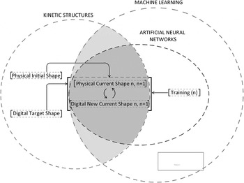
Based on work concluded previously on the automation of kinetic structures, the current paper suggests advancements of such structures by applying automation and optimization logic in the form of ANNs. Figure 1 describes the general framework for readjusting the proposed kinetic system according to ANNs control process. Specifically, the process investigates the current configuration “Physical Current Shape n, n + 1” in each transformation step and simultaneously introduces new final outcomes “Digital New Current Shape n, n + 1” based on the target configuration task “Digital Target Shape.” The ANNs methodology introduced in the training process is included within the machine learning framework (Fig. 1), which represents the continuous feed-forward loop that generates new outcomes in each transformation step and determines the number of training cycles for each feedback scenario “Training (n),” in order to achieve specific adaptive behavior. The continuously updated configurations constitute the input/output parts of the process operating in a reversible manner. The “Physical Current Shape n, n + 1” is defined in the input part of the training process, and in turn this leads to the transformation of a “Digital New Current Shape n, n + 1” (output) that serves as a new input informing the current shape configuration according to given evaluation criteria. The input and output relation is explained further in the following paragraphs, where a comprehensive analysis of the control mechanism is demonstrated.
General framework for the readjustment of kinetic system by the application of control logic.

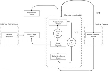
Figure 2 demonstrates a general flowchart of kinetic structure control mechanisms and information flow that describe, in general, the adaptation behavior. The description of information flow starts by feeding the mechanism with initial information with regard to the configuration of structure. The adaptive learning procedure produces new configurations that tend to reach a configuration close to the target one, to be adapted to the conditions of the environment. The training factor that is responsible for the adaptive validation process uses an error elimination statement that plays a fundamental role in the process, because it informs the control mechanism and hence the intelligence of the structure about the divergence from the targeted physical conditions. This divergence is checked against the maximum number of training cycles needed for the training, producing continuously updated configurations in training cycles (n + 1), until this reaches a minimum acceptable error. The performance of a specific kinetic behavior relies on sequential cyclical iterations until a physically optimized shape is reached, which is considered to occur in the current stage k and that is then able to be given a new target configuration in order to be optimized in stage k + 1.
Flowchart of the proposed kinetic structure's control mechanism toward adaptation.

4. STRUCTURAL SYSTEM DEVELOPMENT
4.1. Proposed structure design and control
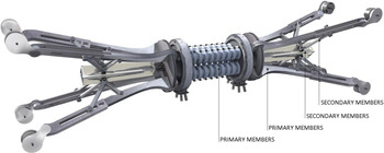
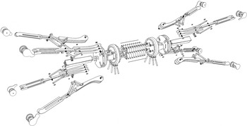
This section investigates the development of the prototype structure as against its physical properties and behavior. In general, kinetic objects need to be able to transform easily and autonomously through information received via control mechanisms so that real-time automation of the members can occur. In terms of kinetic operability, movement between units that are articulately connected can generate variant geometrical configurations in relation to the adaptive design applied (Fig. 3). The geometrical formulation relies on a unit that produces the overall system by repeating itself. In such a scenario, the structure becomes reconfigurable, based on its modular joints control movement (prototype development). Folding abilities are given by the combination of repetitive geometry and modularity, examining, at the same time, a number of infinite solutions that emerge from a respective hierarchical interlocking of the connections at the local prototype level. The process of development incorporates movement as the main design tool, while stressing the necessity to apply kinetic and static conditions to the structure, in order to ensure kinetic controllability during its transformation and rigidness during its operation.
Prototype unit development.

The primary structural mechanism is based on soft components that induce a synergetic transformability of the rigid secondary members, responsible for providing adequate structural stiffness in any operational mode. A central flexible air muscle component acts as a regulator within the reconfiguration process. Connected pneumatic tubes are activated by a proportional airflow pressure regulator and are linked together with diagonal strands that are selectively activated to constitute a multiple-axis reconfigurable unit. For this purpose, the pneumatic actuators are coated and embedded in highly flexible polyurethane cold foam. The elements are self-stabilizing due to their differentiated pressure.
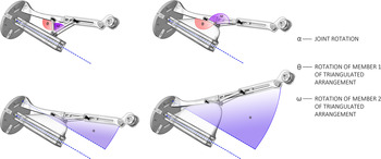
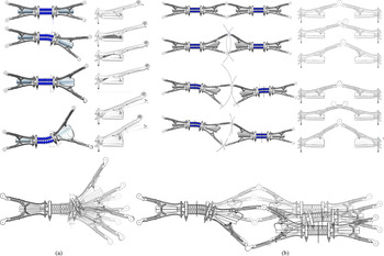
Specifically, the primary structural unit of the typological prototype development consists of four primary members, arranged symmetrically in couples on the longitudinal sides. The primary members are able to alter their length for a respective reconfiguration of the unit. Each joint of the members to adjacent units is provided with a degree of freedom α that enables rotation, that is, a secondary level of movement. Kinematics of the members are enabled by a scissor mechanism that rests on secondary members of the unit. Rotation α of the joints takes place through activation of pressure forces actuated by centrally placed soft pneumatic tubes that induce respective rotations θ, ω of the primary members (Fig. 4). Figure 5 presents the kinetic behavior of the unit at the primary and secondary levels.
Local movement analysis.

Kinetic behavior of units at (a) primary and (b) secondary levels.

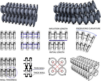
Specifically, the ability of pneumatic tubes to produce axial forces is based on their soft materiality and their capability to be inflated through air channels. Recent research work (Darpa) was conducted at the Department of Chemistry and Chemical Biology of the University of Harvard focusing on the development of soft actuators that are fabricated in organic elastomerics and can produce complex motions in deformation under low stresses (Laschi et al., Reference Laschi, Mazzolai, Cianchetti and Dario2009; Steltz et al., Reference Steltz, Mozeika, Rodenberg, Brown and Jaeger2009; Majidi et al., Reference Majidi, Shepherd, Kramer, Whitesides and Wood2013). The proposed pneumatic tubes operate according to the logic of soft robots and actuators of soft materiality. In the specific prototype, soft elastic tubes form hollow rhombuses with each side, which can be inflated separately and simulated through the development of a hyperelastic skin, as shown in Figure 6. Specifically, each unit is equipped with two pneumatic tubes that control the unit's kinetic performance, locally attached with IPM elastomerics to the primary structural members performing an outward rotation.
Pneumatic tube as an actuator.

Similarly, the intermediate connection between both sides of the unit is designed as a dynamic soft actuator that is able to bend under various pressures operating synergistically to the tubes (Fig. 7). Several studies have focused on the introduction of biologically inspired actuators like elephant trunks. The design of the Bionic Handling Assistant by Festo is able to bend in three dimensions and induce curvatures to the whole system (Festo AG & Co. KG, 2010; Neumann et al., Reference Neumann, Rolf, Reinhart, Queisser and Steil2014). The overall concept is based on unitary actuators with several degrees of freedom. In particular, these are controlled by cables that enable the muscle to stretch and rest under maximum bending moments. The longitudinal section of the air muscle is designed for a vertical bending behavior, while wall thickness manipulation generates elongation to the thinnest walls and a respective curvature to the whole. The overall length of the typological prototype unit is 0.80 m, with central air muscle length of 0.20 m without actuation. When air pressure is supplied, pure elongation and bending behavior of the air muscle takes place extending up to 0.30 m. Furthermore, a refinement of the kinetic mechanism in terms of activation can be achieved by the intermediate connection that enables differentiated air inflation within the soft channels of the mechanism (Fig. 8).
Flexible pneumatic air muscle as a regulator.

Exploded prototype air manipulation.

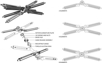
The structural stability of the system is obtained by connecting adjacent unit members with electromagnetic brakes. The devices enable the members’ joints to act rigidly once a reconfiguration of the structure has been obtained (Fig. 9).
Members connection through electromagnetic brakes.

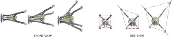
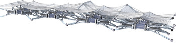
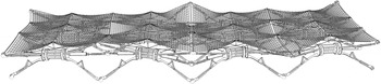
The application of the controlled structure in real terms is based on a feed forward-feedback controller for a quick and responsive transformability. The control scheme applied at the digital level may be extended to an active compliance control mode, which considers over distance sensors, positioning the structural members throughout the reconfiguration process. The compensation of relative differences between the digitally encoded and actual physical positions can be further studied in an exploratory manner that would provide inverse control models, in order to achieve the desired outcomes. In such a unit-based design, the adaptability of the system is explained through the respective articulation of units into an overall configuration, under the influence of specific factors (terrain anomaly, functionality, etc.). Materiality and structural ability serve as the means, allowing natural behavior and overall design transformations to occur. In this framework, various geometrical scenarios and possible uses of the structural system in respect to conditions of the environment could be investigated. A specific scenario of a platform is presented below with (i) deformed at the upper level (Fig. 10) and (ii) aligned at the upper level (Fig. 11).
(i) Platform at deformed level.

(ii) Platform at aligned level.

4.2. Real-time activation through physical/digital transition stages
In this section, physical/digital transition stages as parts of the proposed framework are developed, enabling the connection of physical information with digital data. In this process, sensors collect specific information from the environment and actuator mechanisms transfer the information to the physical world. As a result, a feedback loop between physical/digital data is established that acquires communication between the physical prototype and digital control.
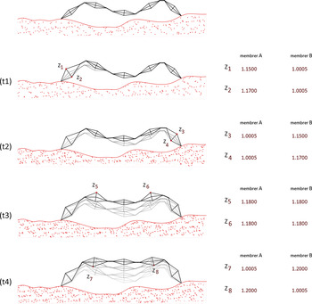
The kinetic structure consists of articulated units that are controlled locally, which in turn results in a rearrangement and transformation of the system at the global level. Two types of adaptation are investigated: internal and external. The external adaptive process focuses on the ability of structures to fit onto a rough terrain, whereas the internal adaptation focuses on the production of various configurations through modular composition and control. Figures 12 and 13 demonstrate how variations of units and the way these are linked together can affect external adaptability onto a rough terrain and can provide meaningful configurations, respectively. In order to control the adaptive design process, transition stages through physical/digital communication must necessarily occur. In order for the control mechanism to perform the learning process, both the target and the initial configurations have to be translated into digital input data.
External adaptation onto a rough terrain through articulated units.

Internal adaptation through variety of configurations.

The physical to digital transition requires the use of distance sensors that collect the highest distance of units from the ground represented as points in the digital environment. These values inform the digital environment about the current state of structure, while the desired configuration is represented as Z values to be reached. As already explained, both transition stages are equally related to the structural substance of the physical prototype. Hence, the digital to physical transition stage is responsible for validating the adaptive results by informing the physical prototype about the new digital configuration. In terms of activation, the kinetic ability of the structure is investigated by applying kinematic and soft materiality principles, which can be considered to be optimized techniques, in relation to energy consumption. The scissorlike structure is controlled through the airflow activation of pneumatic elements causing transformation and, therefore, a new configuration of the structure. In order for this transition to occur, each unit uses air pump motors that enable specific variations. In a digital environment, values are represented by a length factor from 1.0005 to 1.2000, while in real-time, these values are decoded according to the required length of the structural members, calculating the duration of airflow used in the actuator mechanism. Through a feedback loop process that continually evolves, the error is calculated until it is eliminated and the structure reaches the desired configuration goals.
5. CONTROL MECHANISM DEVELOPMENT
5.1. Mathematical model and algorithmic control
The ANNs algorithm was selected over other automation and optimization methods due to its ability to optimize and improve a given state of structure into a target one by achieving a specific sequence of movements. In this case, the target configuration is predefined as a result of external adaptation, leading to the application of a supervised method of learning using predefined outputs. As already mentioned, McCulloch and Pitts's (Reference McCulloch and Pitts1943) general threshold model provides information about the basic logic of ANNs that is informed by other activation functions, such as sigmoid. This work, looks into the feedforward neural network algorithm that defines the propagation procedure in a linear manner. According to this approach, which was initially proposed by Werbos (Reference Werbos1974), the information is passed through layers until the final outputs are reached. Specifically in this case study, a single-layer perceptron that was demonstrated by Donald Hebb (Reference Hebb1949) is introduced, aiming to optimize structural capacity using one layer while this is informed by backpropagation Hopfield's logic.
In particular, a typical ANNs algorithm can be graphically represented as a set of nodes together with the connections established between them. The overall control mechanism concept is based on the identification and definition of the inputs on which specific values are applied that differentiate the initial ones in terms of strength and their influence on the general process. Then, the sum of strengthened values is passed through an activation function, in order to compute the variation in each neuron. The proposed working flow validates the ability of a system to be adaptive as nodes are updated by new ones upon repetition, to fit the initial target configuration goals.
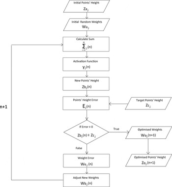
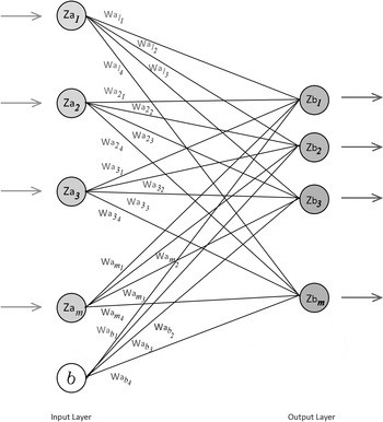
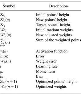
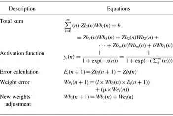
The translation of the structure's configuration into the algorithm is a fundamental part of the procedure for monitoring purposes, in order to provide meaningful results. The configuration is represented by a fixed amount of points (i) that move into the Z-axis representing the overall shape. The process allows alteration of the points’ height, resulting in a transformation of the overall shape, until the target shape is achieved. Figure 14, presents a comprehensive flowchart of the adaptive process based on the ANNs methodology. According to this, input data of initial points’ height are initialized (Za i), while random strength is applied in each input, called “weight” (Wa i). Weights play a major role in the control mechanism because they define the validity in each node and are able to update and adjust themselves each time, according to the expected results; the overall process can be called adaptive (Engelbrecht, Reference Engelbrecht2007). The signals are then propagated through the network to be summed up ( $\sum\nolimits _{i = 0}^m \lpar n \rpar $) and are provided as input through a sigmoid activation function (y i(n)) that calculates the output of each neuron. Sigmoid function is nonlinear, increasing and exhibiting smoothness, because values that passed through vary from 0 to 1; in the case of a gradient-based system that serves into mapping, those values to the length factors range from 1.0005 to 1.2000 (Kostanic & Ham, Reference Kostanic and Ham2000). Subsequently, new value results are the current points’ position (Zb i(n)), representing the real-time configuration of the structure, which is then processed to define error divergence (E i(n)) in proportion to the desirable configuration. It is in turn translated to target points’ height (Zc i). The control mechanism process is being increasingly repeated (n + 1) until the error is eliminated in weights (We i(n + 1)) by fitting the appropriate weights in the points’ position. The process of repetition updates weights (Wb i(n + 1)) by propagating errors backward to the algorithm with the updated weights into Sum equation until optimized point's height (Zo i(n + 1)) and weights (Wo i(n + 1)) are produced. Tables 1 and 2 illustrate the respective symbols and equations used. Figure 15 presents the proposed single-layer perceptron together with the network of the structure's inputs and outputs.
Comprehensive flowchart of the adaptive design process based on artificial neural networks (ANNs).

The architecture of artificial neural networks (ANNs) single-layer perceptron.

Symbols and equations of control mechanisms

Note: Here, i is the number of input points, n is the number of training cycles, and k is the number of tasks solved.
Control mechanism's equations used

5.2. CASE STUDIES AND RESULTS OF SIMULATION
The geometrical configuration of the proposed adaptive behavior is controlled through the parametric-associative design software Grasshopper (plug-in for Rhino) and Kangaroo (plug-in for Grasshopper). The kinetic behavior of the proposed digital design model on control based on ANNs is examined through the simulation process. Overall, the simulation is based on two stages; initially, the simulation focuses on the distribution of stresses in order to visualize the kinetic and structural behavior of the system; this is achieved through manual control (Fleischmann et al., Reference Fleischmann, Knippers, Lienhard, Menges, Schleicher and Menges2012; Fleischmann & Menges, Reference Fleischmann and Menges2012). In the next stage, the kinetic transformation is controlled through the ANNs automation method connecting Grasshopper and Processing (Java-based language) to send and receive data updating the initial configuration shape.
5.2.1. Stage 1: Simulation of digital prototype through parametric associative control
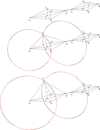
The physical behavior of the proposed prototype at the local and global levels can be achieved by applying a number of forces using the Kangaroo software. The structural definition of the system relies on airflow that transforms primary members’ length and rotation due to its connectivity with other units. In the simulation process, the geometrical definition relies on spring behavior with the start length being equal to a scaled rest length. Each two nearby scissorlike structural units perform together, having the same members’ end points, and therefore, each transformation affects each other's end point. Actuation in a digital level occurs through a value that scales the length of the member in a specific unit, while it simultaneously finds the intersection point between the two circles with radius equal to each member's length (Fig. 16). The overall simulation is based on Hooke's law of spring forces (Ahlquist & Menges, Reference Ahlquist, Menges, Ceccato, Hesselgren, Pauly, Pottmann and Wallner2010; Phocas et al., Reference Phocas, Kontovourkis and Ioannou2012), which are applied aiming to capture a simplified form of the proposed system's physical behavior for training purposes. More specifically, opposite end points of structural units’ members are connected through linear springs by equal start and rest lengths performing as the in-between member of transformation. This enables stiffness of the scissor-like units and, in turn, stabilization of the overall structure in any state of transformation while acting in compression. Furthermore, a physical behavior in the frame of the digital environment simulation is expected to be achieved, and therefore, gravity force and ground collision (using a three-dimensional surface) are applied in each start and end point of the unit members. The overall control of the system is achieved through local control of the scissors-like members’ length, leading to the transformation of the initial configuration until this reaches the final appropriate configuration. Figure 17 represents various simulations of the digital prototype through parametric control of local structural members, resulting in different configuration states during the transformation.
Geometrical definition and parametric control of nearby scissorlike structural units.

Digital simulation of a proposed prototype through parametric associative control.

5.2.2. Stage 2: Digital prototype simulation through ANNs algorithm
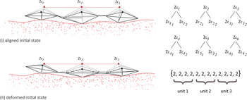
At a further stage, the control mechanism has been developed in Processing (programming language) according to the ANNs basic algorithm operating together with Grasshopper (plug-in for Rhino) in order to automate the kinematic behavior of the proposed system. The aforementioned simulation process is extensively implemented through gHowl (plug-in for Grasshopper) and UDP (library for Processing), which are both based on the UDP send/receive method enabling real-time communication between the two main programs (Grasshopper and Processing). Processing serves as the processor of the structural geometrical adaptability, sending the length scaling values to Grasshopper, where the simulation in digital environment occurred. When a transformation is applied on the system, the new Z values of the intersection points are sent back to Processing, so that the error is calculated and new weights are applied in order for the new scaling values to be received by the Grasshopper in training cycle (n + 1; Fig. 18). A port is initialized between the two programs in order for them to communicate. In Grasshopper the UDP receiver is set in the beginning of the algorithmic definition that receives information in the form of strings from Processing. The values are converted to float numbers so that units’ Z values can be manipulated in the Grasshopper environment. In order to send updated data back to Processing in the form of strings, a UDP send is being initialized at the end of the algorithmic definition.
Units alignment: (i) aligned initial state and (ii) deformed initial state.

In the opposite direction, in Processing the data is stored in an array so that the calculation for each point is performed and then a UDP send is sending the refined data back to Grasshopper. Using this process, the configuration of an initial shape is explained and reviewed in detail, by examining specific experiments based on four steps.
Step 1: Introduction to the case study
The learning process is based on the structure's current state alternating with a new adaptive configuration that responds automatically to the stimuli of the environment. The structure differentiates its initial configuration, expecting appropriate configuration shapes. The investigation gradually moves toward complex ones aiming to examine the accuracy of the training process as well as the rate of success obtained in the digital environment. Therefore, target configuration experiments are investigated using different parameters.
Step 2: Initial configuration shape
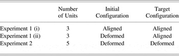
The first experiment focuses on the alignment of units in an initial configuration shape. This is investigated through various initial shapes; (i) units are initially lined up (Zc 1 = Zc 2 = Zc 3) and (ii) units are initially in a deformed position (Zc 1 ≠ Zc 2 ≠ Zc 3) (Table 3). The target configuration is given as an array of 12 values in pairs representing pairs of primary members that operate together, for example,  $Z{c_{{1_1}}},\;Z{c_{{1_2}}}$, while four members represent a single unit (front Zc 1, back Zc 4 for unit 1; Fig. 18).
Case study experiments

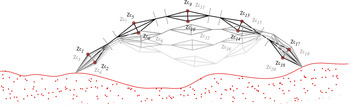
In the second experiment, a curvelike configuration functions as the target shape that needs to be obtained. The upper and the lower height values of the connections of the scissorlike members are given a defined value to be reached. They are initialized as an array consisting of 40 values upper front (Zc 1, Zc 5, Zc 9, Zc 13, Zc 17), upper back (Zc 3, Zc 7, Zc 11, Zc 15, Zc 19), lower front (Zc 2, Zc 6, Zc 10, Zc 14, Zc 18), and lower back (Zc 4, Zc 8, Zc 12, Zc 16, Zc 20). An equal number of weights is applied as strength on initial points, which by sequence based logic, generate new states of structure gradually reaching the final appropriate position (Fig. 19).
Units alignment: deformed initial state/deformed target state.

Step 3: Expected appropriate configuration shape
Through the training, new current shapes are expected to be obtained in each step in which a total percentage error is calculated according to the expected appropriate configuration shape. In Experiment 1 (ii) members with identity numbers 1, 6, 7, 8, 9, 10, 11, and 12 are expected to approach the configuration at a quicker rate than others, whereas in Experiment 2 members 11 and 12 are expected to be the slowest. This difference occurs not only because of the shapes given (i.e., the initial and expected state) but also because of the amount of learning rate. Subsequently, the lowest learning rate defined, the longest the time needed to achieve a final optimized shape. The relationship between learning rates and time needed for optimization is examined in the following experiments.
Step 4: Test results review. In Experiment 1 (i)
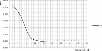
Parameters: Momentum 0.1, Learning Rate 1, Target Points 0.9, Initial Points 1.0005
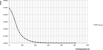
Parameters: Momentum 0.1, Learning Rate 0.1, Target Points 0.9, Initial Points 1.0005
Experiment 1 (i) is examined by applying a different value in the learning rate parameter. The overall error progress in relation to training cycles (n) is illustrated through graphs that represent the training process of the structure (Figs. 20 and 21). As the learning rate parameter decreases from 1 to 0.1, the learning curve acquires a smoother result, passing through all the different states (a tenfold number of intermediate states and attempts) that had overtaken before, while reaching negative error values (Fig. 21). In this experiment, the error is gradually eliminated at an early stage (one-quarter of the total number of iterations), which proves an early approach of the target configuration (100 attempts – n); in the rest of the iterations it approaches error 0, and thus an optimized shape is reached. Therefore, the learning rate affects the kinematic optimization strategy of geometrical exploration. A lower value is suggested to be used in complex experiments, whereas the difference between transformations is slight and might be passed by, without any result.
Average error progress in relation to training cycles (n) – L.R. 1.

Average error progress in relation to training cycles (n) – L.R. 0.1.

In Experiment 1 (ii),
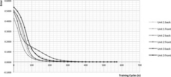
Parameters: Momentum 0.1, Learning Rate 0.1, Target Points 0.9,
Initial Points {1.2, 1.2, 1.2, 1.2, 1.1557, 1.0864, 1.1060, 1.1241, 1.0936, 1.0725, 1.2, 1.0005}
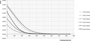
Parameters: Momentum 0.1, Learning Rate 0.1, Target Points 0.5,
Initial Points {1.2, 1.2, 1.2, 1.2, 1.1557, 1.0864, 1.1060, 1.1241, 1.0936, 1.0725, 1.2, 1.0005}
In Experiment 1 (ii) the transformation from a deformed state to an aligned one is conducted. The target position varies between 0.9 and 0.5, and errors of each joint position (E1–E12) in relation to training cycles (n) are illustrated in the graph (Figs. 22, 23). As it can be observed, in the second case, many more iterations are conducted (849) than in the first one (571), even though the initial position requires a smaller transformation in relation to the other one. This occurs due to their ability of improving gradually at a quicker rate in larger errors, while in the second case, values alter at a smaller extent according to the overall state of the structure, demonstrating a smoother error progress.
Error elimination progress of each unit in relation to training cycles (n) – T.P. 0.9.

Error elimination progress of each unit in relation to training cycles (n) – T.P. 0.5.

In Experiment 2,
Parameters: Momentum 0.1, Learning Rate 0.1
Initial Points: 1.0005
Target Points {1.4, 1.4, −0.9, −0.9, 1.1, 1.1, −1.1, −1.1, 4.5, 4.5, 1.8, 1.8, 3.6, 3.6, 1.3, 1.3, 5.3, 5.3, 3.5, 3.5, 5.2, 5.2, 2.5, 2.5, 5.4, 5.4, 3.2, 3.2, 5, 5, 2.2, 2.2, 2.4, 2.4, 0.5, 0.5, 1.3, 1.3, −0.5, −0.5}
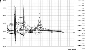
The final Experiment (2) examines the transformation levels of an initial deformed shape to a target deformed configuration by comparing their error values and, therefore, their learning progress. The five units initiated in the experiment consisting of 20 joints (up and down) along with the rest 20 in the back of the units are imported in the algorithm as 40 members to be applied random weights until they reach their target position. An initial deformed position at minimum value of 1.0005 is given to all members because they have no deformation at the local level (units) although they perform an overall deformed configuration. The overall training process holds 2926 attempts (n) until it reaches the final optimized shape. During the process, high rate error values (350 n, 750 n, and 1500 n), positive and negative, are presented even when the overall process appears to exhibit improvement in eliminating the error (Fig. 24). This occurs due to the ability of the system to be treated as a whole in a parametric associative logic in a physical-based context (Kangaroo forces, gravity, etc.). The specific chainlike configuration is transformed continuously without being able to hold the position in one of the units’ joints, even though it reaches zero (E35,36, E37,38) at a relatively early stage, due to its ability to affect the overall system transformation. In order for an error elimination to occur in the joints (E1–E40), an average position between them is necessary (1500 attempt – n), which gradually gives an improved stage until each unit and overall configuration reach their final position.
Error elimination progress of each unit in relation to training cycles (n).

The results obtained from the various case studies show that the applied ANNs optimizing strategy for structural transformation manages to obtain an average final appropriate configuration at an early number of training cycles, while in the rest of training cycles, it tends to reach the actual final appropriate configuration by eliminating the error in every input. In this framework, the applied methodology might be characterized as highly accurate, demanding the evaluation of ANNs performance through a validation procedure in order to compare training and validation errors as well as to provide feedback and control of the overall training/optimization process. Nevertheless, at this stage of investigation, the study focuses on the optimization of the structure's transformation process until a final appropriate configuration is reached in respect to a target configuration and not on the investigation of the performance of the ANNs methodology, which can be investigated in a future study.
6. CONCLUSIONS
This work demonstrates the automate optimization process where the kinetic transformation stages of an adaptive structure are dominated by a machine learning control mechanism based on ANNs in order to explore suitable solutions of final appropriate shapes.
The suggested design of the adaptive kinetic structure focuses on the formulation of a system consisting of individual articulated structural units composed sequentially and formulated through a primary structural mechanism based on soft components and secondary rigid members. The combination of soft and rigid structural components allows the synergetic transformability of units, in contrast to the adequate stiffness of the structural members in any operational mode. The application of the proposed machine learning mechanism based on ANNs achieves the effective control of the complex and nonlinear transformation behavior of the system at the global level, as a result of the units’ local activation that further influences nearby units in a disorganized and uncertain way. In addition, the mechanism is capable of handling a large amount of input data, allowing at the same time the optimization of the structure's position and, hence, its configuration in any transformation stage.
The analyses conducted show that the control methodology used can satisfy the adaptive criteria specified according to the given unstructured environments and conditions. By combining the local activation and control mechanism of the structure with the ANNs algorithmic search procedure, an effective and nonexpensive process to compute a large amount of information and search for suitable solutions that adapt to given conditions can be achieved in a short time period. In addition, the suggested methodology might provide a fast, accurate, and reliable method for alternatives moving toward adaptive and reconfigurable kinetic structures achieving solutions in cases where the design and structural objectives require the search of optimal form at the global level through nonlinear local control and investigation.
Finally, the findings show that although the proposed methodology managed to reach an average final appropriate configuration at an early number of training cycles, the evaluation of the ANNs performance through a validation procedure necessitates further examination and investigation, by comparing training and validation errors. In addition, further studies might include the physical development and evaluation of the structural prototype and control mechanism. These may concern related issues of movement and geometrical restrictions of the members transformations and control integration with regard to sensors and motion planning.
Odysseas Kontovourkis is a Lecturer in architectural communication media in the Department of Architecture at the University of Cyprus. His research and teaching interests focus on the integration of computational design and fabrication strategies with the architectural design process aiming at the optimization of architectural design and construction according to functional, structural, environmental, and morphological architectural design criteria. Dr. Kontovourkis's current research covers the fields of digital architectural design based on generative and parametric processes, digital fabrication strategies, and human movement behavior simulation with an emphasis on pedestrian modeling in the built environment.
Marios C. Phocas is an Associate Professor in the Department of Architecture at the University of Cyprus, as well as Coprincipal of the Archimedes Research Center for Structural and Construction Technology. From 2006 until 2013 he served as Interim Head of the Department of Architecture. Prior to his appointment at the University of Cyprus, he held posts in teaching and research at the Institute of Building Structures and Structural Design of the University of Stuttgart from 1996 until 2004. Dr. Phocas has authored several publications in integrated architectural design, kinetic structures, and earthquake-resistant structural building design.
Ifigenia Lamprou was a Teaching Assistant–Postgraduate Associate under the supervision of Dr. Odysseas Kontovourkis, where she was the Coordinator for the laboratories on three-dimensional printing and laser cutting in the Department of Architecture at the University of Cyprus. She received her BS in architecture and Diploma in architecture engineering from the University of Cyprus. Her research interests focus on generative design, parametric-associative logic, and computer-aided design.