Do low-income households systematically face higher inflation than high-income households? This question has gained urgency as inflation reached multi-decade highs in 2021–2022. The prevailing finding, based on analyses using the Consumer Price Index (CPI), has been substantial and persistent differences in inflation experiences across the income distribution.
The CPI-based literature has evolved considerably over time (see Jaravel (Reference Jaravel2021) for a review). Early studies found modest differences across income groups.Footnote 1 McGranahan and Paulson (Reference McGranahan and Paulson2006) concluded that “the CPI-U does a reasonable job of measuring the inflation experience of the demographic groups we investigate.” Recent work consistently finds that low-income households face meaningfully higher inflation rates, relying on reweighting CPI elementary indices to reflect different budget compositions.Footnote 2 While methodologically sound, this approach faces scope limitations if trying to apply results to national accounts aggregates.
These limitations stem from a critical feature of the CPI: it captures mostly out-of-pocket consumer spending and does not represent total aggregate expenditure. For this reason, we revisit and extend the discussion of inflation inequality to the Personal Consumption Expenditure (PCE) price index from the U.S. national accounts. This measure, which the Federal Reserve prefers (Board of Governors of the Federal Reserve System, 2024), includes expenditures on government-provided health care (e.g., Medicare and Medicaid), imputed financial services (like the consumption value of “free checking”), and other categories absent from household surveys (Garner et al. Reference Garner, Martin, Matsumoto and Curtin2025). Moreover, alignment with national accounts aggregates mitigates concerns about under-reporting in surveys that could bias CPI weights (National Research Council, 2022).
To measure inflation inequality consistent with aggregate income and expenditures, we build on previous research creating a new joint distribution of income and consumption (Gindelsky, Reference Gindelsky2024; Garner et al. Reference Garner, Martin, Matsumoto and Curtin2025; Gindelsky and Martin, Reference Gindelsky and Martin2025). We integrate the Bureau of Economic Analysis’ (BEA) income distributions with the Bureau of Labor Statistics’ (BLS) detailed expenditure distributions. We then construct the first, national accounts consistent, income-stratified PCE price indices (IS-PCEPX) by disposable personal income (DPI) for 2000–2023.Footnote 3 Like many previous CPI studies, we calculate the IS-PCEPX by reweighting a common set of elementary indexes for different income groups. The limitations to this approach are discussed further in Section 3.
Our findings reveal that PCE inflation inequality is smaller and more dynamic than CPI-based studies suggest. During 2000–2012, the bottom income decile experienced annualized inflation of 0.3 percentage points higher than the top decile. However, this pattern reversed during 2012–2023, with the bottom decile experiencing less inflation than the top decile, driven primarily by rapid price growth in financial services and insurance (3.4% annually) that disproportionately affects higher-income households. We subsequently decompose differences in PCE- and CPI-based inflation inequality measures into ranking, formula, and scope effects.
The paper proceeds as follows. Section 1 describes our methodology for constructing indices and integrating income and expenditure distributions. Section 2 presents inflation patterns and real income growth across income groups, emphasizing changes across time periods, and compares our PCE-based measures with CPI-based approaches. Section 3 concludes.
1. Methodology
Our approach to constructing IS-PCEPX requires integrating two complex datasets: BEA’s distributional personal income estimates and BLS’s distributional PCE estimates. This section provides an overview of our data sources and prior methodology, then details the construction of our new IS-PCEPX using the chained Fisher formula.
1.1. Data sources overview
Our analysis covers 2000–2023, constrained by the availability of integrated distributional estimates. The underlying data sources include the Current Population Survey Annual Social and Economic Supplement (CPS-ASEC) (for demographics and income) and Consumer Expenditure Survey (CE) (for spending patterns), augmented with various administrative sources for transfer programs and business income.
We construct both quintile and decile groupings based on equivalized DPI. All estimates use CPS-ASEC survey weights adjusted to account for the multiple imputation process and scaled to match national population totals.
1.2. Income distribution
The foundation of our analysis rests on BEA’s distributional personal income estimates. BEA’s methodology, detailed in Gindelsky (Reference Gindelsky2024), allocates approximately 75 distinct components of personal income from the National Income and Product Accounts (NIPAs) to households in the CPS-ASEC. Each component is distributed to households so that the weighted sums match aggregate totals from the NIPAs. The resulting totals, PI and DPI, are equivalized by dividing by the square root of household size, in order to compare households of different sizes to each other. Income quantiles are assigned based on equivalized income.
1.3. Expenditure distribution
The BLS’s distributional PCE research methodology, described in Garner et al. (Reference Garner, Martin, Matsumoto and Curtin2025), transforms CE survey data to align with national accounts definitions and totals.Footnote 4 BLS maps approximately 600 CE spending categories to 150 detailed PCE categories, addressing definitional differences—for example, CE captures out-of-pocket medical expenses while PCE includes third-party payments like Medicare and Medicaid. External data are used to impute expenditures for categories that are either out-of-scope or not well-covered in the CE, including third-party health care, financial services, and non-profit institution expenditures.Footnote 5 A Pareto-based top-tail adjustment (recommended by Zwijnenburg et al. (Reference Zwijnenburg, Grilli and Engelbrecht2022)) is intended to mitigate bias from high-expenditure households’ lower survey participation and under-reporting in the CE. Finally, all estimates are scaled so their weighted sums match official PCE aggregates category-by-category, ensuring consistency with national accounts while preserving observed expenditure heterogeneity.
This process yields PCE imputations for 150 product categories—somewhat aggregated from the 244 detailed products in NIPA tables but providing sufficient detail to capture key heterogeneity in categories like financial services and insurance. Some detailed patterns, such as different relative amounts spent on foreign and domestic auto across income groups, are not captured due to data limitations, but the framework reflects the essential drivers of distributional differences while maintaining data quality.
1.4. Integration method
Integrating the personal income and PCE distributions requires harmonizing two datasets with different sampling frames, definitions, and methodologies. We follow the approach developed in Gindelsky and Martin (Reference Gindelsky and Martin2025).
We begin by constructing comparable income aggregates in both datasets by selecting concepts that are comparably defined in both surveys, including wages, salaries, self-employment, interest, dividends, and Social Security. We scale each to align with NIPA totals. This comparable income excludes certain PI components (like imputed financial services) that have no clear counterpart in the CE.Footnote 6
We then employ multiple imputation with predictive mean matching to impute most category-level PCE to households in the CPS-ASEC (a few exceptions are discussed below). The predictive model incorporates key demographic and economic characteristics of reference persons: age, race, education, family size, urban residence indicator, and income source composition indicators (wages, self-employment, Social Security, etc.).
The matching process is constrained to ensure realistic donor-recipient pairs. Specifically, we only match households within the same decile of equivalized comparable income and the same housing tenure category (owner vs. renter). This ensures that expenditure patterns are imputed from households with similar economic circumstances and housing costs.Footnote 7
We handle overlapping concepts carefully to maintain consistency between income and expenditure sides. For example, rather than imputing third-party health expenditures from the CE, we allocate the health care components of personal income (Medicare, Medicaid, employer contributions) across PCE categories. Similarly, we replace PI rental income from owned housing with imputed rental equivalence from the CE to ensure housing costs are treated consistently. For more details, see Gindelsky and Martin (Reference Gindelsky and Martin2025).
1.5. Index construction
With integrated datasets providing income quantile specific expenditure shares, we construct income-stratified PCE price indices following a similar approach to Klick and Stockburger (Reference Klick and Stockburger2024) and Jaravel (Reference Jaravel2026)’s method of re-weighting CPIs. We re-aggregate the detailed PCE subindices from NIPA Table 2.4.4U using household group-specific expenditure shares. Most of these indices are themselves based on consumer price indices or producer price indices produced by BLS (Bureau of Economic Analysis, 2024). Combining weights from adjacent years, we adhere to the BEA’s methodology of using the chained Fisher formula, which is the geometric average of the well-known Laspeyres and Paasche formulas.
The Fisher formula for group
 $g$
’s inflation in year
 $t$
relative to year
 $t-1$
is:
 \begin{equation} P^F_{gt} = \sqrt {\left (\sum _i s_{i,t-1,g} \left (\frac {p_{it}}{p_{i,t-1}}\right )\right )\left (\sum _i s_{itg} \left (\frac {p_{it}}{p_{i,t-1}}\right )^{-1}\right )^{-1}}, \end{equation}
where
 $s_{itg} = x_{itg}/\sum _i x_{itg}$
represents group
 $g$
’s expenditure share for detailed product
 $i$
in year
 $t$
,
 $x_{itg}$
is group
 $g$
’s PCE for product
 $i$
, and
 $p_{it}$
represents the product’s PCE price index from NIPA Table 2.4.4U.
Crucially, the price relatives
 $p_{it}/p_{i,t-1}$
are identical across all income groups due to limitations in the source data underlying the
 $p_{it}$
—these represent the full population and so the group subscript is omitted. Differences in inflation across income groups arise solely from the interplay between group-specific expenditure shares (
 $s_{itg}$
) and product-specific inflation rates.
As discussed above in the previous subsection, our set of categories is somewhat aggregated from the 244 detailed products in the NIPA tables. Some detailed PCE categories have no counterpart in the CE (such as those for non-profit institutions serving households), and some are more disaggregated in the PCE (such as foreign and domestic autos), or are particularly noisy in survey data (such as pleasure aircraft). In some cases, therefore, our indices reflect expenditure share differences by group at the more aggregated level (like new automobiles), but do not reflect detailed patterns such as different foreign vs. domestic compositions by group.
While the main IS-PCEPX are constructed using the Fisher formula, we use a couple of other index formulas for supplementary analyses. First, the first decile to tenth decile inflation gap decompositions in Figure 2 are based on the Tornqvist formula, written
 \begin{equation} P^T_{gt} = \exp {\left \{\sum _i 0.5\left (s_{i,t-1,g}+s_{itg}\right )\ln {\left (p_{it}/p_{i,t-1}\right )}\right \}} \end{equation}
We use the Tornqvist here due to the advantages of its multiplicative form. The Tornqvist and the Fisher second-order approximate each other (Diewert, Reference Diewert1978).Footnote
8
The gap (in natural logs) between groups
 $g$
and
 $g'$
is then additive across categories as
 \begin{equation} \ln P^T_{gt} - \ln P^T_{g't} = \sum _i \Delta w_{it,g,g'}\ln {\left (\frac {p_{it}}{p_{i,t-1}}\right )}, \end{equation}
where
 $\Delta w_{it,g,g'} = 0.5\left (s_{i,t-1,g}+s_{itg}\right ) - 0.5\left (s_{i,t-1,g'}+s_{itg'}\right )$
.
Table 2 uses the Lowe (or modified Laspeyres) formula to estimate the impact of scope, weight, and other methodology differences between the IS-PCEPX and related CPIs by holding index formula constant. The Lowe can be written
 \begin{equation} P^{Lo}_{gt} = \sum _i s_{i,b,t-1,g} \left (\frac {p_{it}}{p_{i,t-1}}\right )\!, \end{equation}
where
 $b$
is an earlier weight reference period and
 \begin{equation} s_{i,b,t-1,g} =\left ( x_{ibg}\frac {p_{i,t-1}}{p_{i,b}}\right )/\sum _i \left (x_{ibg}\frac {p_{i,t-1}}{p_{i,b}}\right ) \end{equation}
are period-
 $b$
expenditure shares which have been adjusted to reflect price change from
 $b$
to year
 $t-1$
.Footnote
9
Unlike the Fisher or Tornqvist, the Lowe has fixed expenditure weights that do not account for consumer substitutions in the face of relative price change (Bureau of Labor Statistics, 2023).
2. Results
Our IS-PCEPX reveal a more nuanced picture of inflation inequality than suggested by previous CPI-based studies. While we confirm that lower-income households face higher inflation rates on average, the differences are substantially smaller and have been converging over time. This section presents our main findings on inflation patterns across income groups, changes over different time periods, and the underlying drivers of these patterns.
2.1. Overall inflation patterns across income groups
The overall pattern of IS-PCEPX confirms that lower-income households face higher inflation, but the gradient is modest. Over the full 2000–2023 period, annualized inflation ranged from 2.28% for the bottom quintile to 2.15% for the fourth quintile, before rising slightly to 2.21% for the top quintile. The maximum difference between any two quintiles is just 0.13 percentage points annually—substantially smaller than differences found in CPI-based studies.
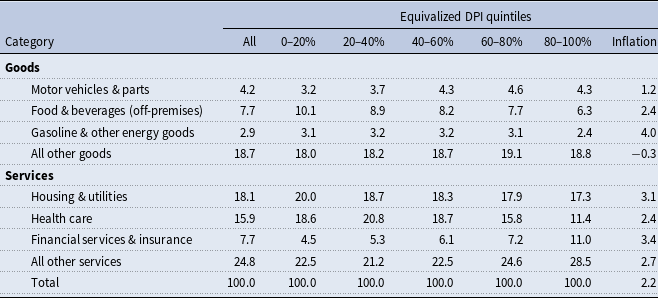
PCE composition and inflation, 2000–2023 all values are expressed as percentages

Note: The first part of this table provides the composition of Personal Consumption Expenditures (PCE), in major categories, for all households, and then by quintile, as ranked on equivalized Disposable Personal Income (DPI). The numbers are averages for the full period (2000–2023). The final column provides the annualized change in the PCE price index from 2000–2023 for each item.
Table 1 shows the composition of PCE expenditure and inflation rates by major category over our full sample period (2000–2023), revealing the expenditure patterns that drive these inflation differences.Footnote 10 The data reveal several components with relatively low variation across the income distribution (such as gas and motor vehicles) and others with significant heterogeneity. Lower-income households devote larger expenditure shares to necessities with moderate inflation rates: food and beverages represent 10.1% of expenditures for the bottom quintile compared to 6.3% for the top quintile, while housing and utilities account for 20.0% versus 17.3%, respectively.
Conversely, higher-income households allocate substantially more to categories that experienced rapid price growth. Financial services and insurance represent 11.0% of top-quintile expenditures but only 4.5% for the bottom quintile—a 2.4-fold difference. This category experienced fast inflation over the sample period at 3.4% annually, significantly exceeding the 2.2% average PCE inflation rate calculated for this period. Health care shows the opposite pattern, accounting for 18.6% of bottom-quintile expenditures versus 11.4% for the top quintile, with inflation of 2.4% annually.
2.2. Comparison to CPI
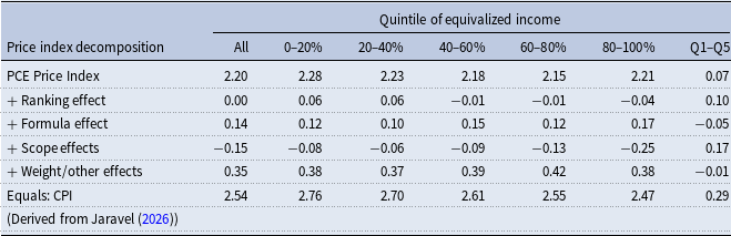
Next, we seek to explain the differences between our results and the significantly larger inflation gaps between quintiles found by Jaravel (Reference Jaravel2026) using the CPI. Table 2 provides a decomposition of these differences.
Price index decomposition (2002–2023) all values are expressed as percentages

Note: This table provides data users a decomposition of the differences between the Personal Consumption Expenditures (PCE) price index and the Consumer Price Index (CPI), as applied to the current exercise, both for the full population and the stratification by quintile. Q1–Q5 refers to the gap between the bottom and the top quintile. The PCE Price index for All is the official BEA measure. The overall decomposition is extended to the quintile level, beginning with quintiles constructed using equivalized DPI, and then subsequently reconstructed for each row. The final row is CPI, ranked on equivalized family income as defined in the CE, as reconstructed from the data files provided as part of the Distributional CPI (D-CPI) project (Jaravel, Reference Jaravel2026). Beginning with PCE, the first adjustment is change in average inflation due to the “ranking effect”, from calculating the IS-PCEPX by CE family income using the CE rather than DPI in the CPS. Next, the “formula effect” is derived from re-calculating the IS-PCEPX using the CPI’s Lowe formula. Next, the “scope effect” refers to including (excluding) items definitionally in CPI (PCE) to reconcile the indices. Finally, “weight/other effects” is computed as the remainder between the scope-adjusted IS-PCEPX and the indices constructed from the Jaravel (Reference Jaravel2026) replication files. This residual reflects the impacts (once all the other adjustments are accounted for) of different source data for the weights and for the few cases in which PCE and CPI use different price indices, such as gasoline and airfare.
The CPI shows much larger average differences across income groups (last row of Table 2), with the bottom quintile experiencing 2.76% annual inflation compared to 2.47% for the top quintile—a gap of 0.29 percentage points, more than four times as large as our PCE-based findings. However, the CPI differs from the IS-PCEPX among many dimensions including formula, expenditure scope, and weights.
The decomposition in Table 2 is constructed by re-calculating the IS-PCEPX sequentially and measuring the difference in average annual inflation between steps.Footnote 11 The first step, using estimates based on the CE, is to compute IS-PCEPX by quintile of equivalized CE income (as done in Jaravel (Reference Jaravel2026) and Klick and Stockburger (Reference Klick and Stockburger2024)), thereby estimating the impact of ranking on this versus DPI and on using the CE versus the CPS.Footnote 12 Then, the formula effect is estimated by changing the formula from the Fisher to the Lowe (4), similar to McCully et al. (Reference McCully, Moyer and Stewart2007), matching also the biennial or annual weight reference periods of the CPI. The scope effect is estimated by re-calculating the index after dropping categories not included in the CPI (see Table A3) and adding back in categories not included in the PCE (see Table A4).Footnote 13 Finally, even after adjusting for scope, the IS-PCEPX and CPIs differ due to data sources used for the weights (McCully et al. Reference McCully, Moyer and Stewart2007; Garner et al. Reference Garner, Martin, Matsumoto and Curtin2025), the elementary price indices for gasoline and airline fares, some seasonal adjustment differences, and to small degrees due to data frequency.Footnote 14
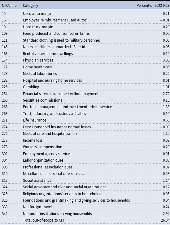
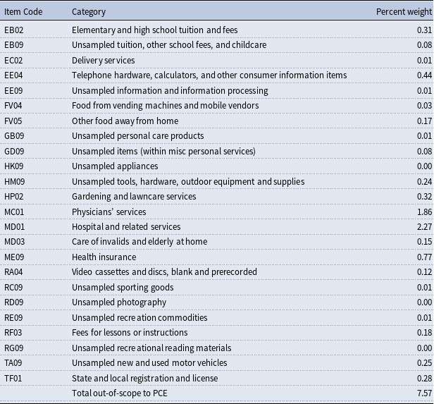
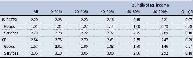
The decomposition in Table 2 reveals that while weight effects are most important for the average difference in IS-PCEPX and CPI inflation across all groups, scope effects (differences in what categories are included) account for much of this divergence in the pattern of inflation differences across groups (−0.08 percentage points per year for the bottom quintile, but over three times as large at −0.25 for the top quintile). Table 3 delves deeper into the issue of scope when comparing IS-PCEPX and CPI by income quintiles. Table 3 displays average IS-PCEPX inflation by quintile both overall and separately for categories which overlap with CPI and categories which do not. Excluding non-CPI categories, the average Q1–Q5 gap for the IS-PCEPX is much closer (0.23 pp), while the gap for the non-CPI categories has the opposite sign and is larger in magnitude (−0.38). Additionally, Table A5 separates both the IS-PCEPX and CPI into goods and services subcategories. Level differences in inflation exist across all categories and quintiles, but services (driven by financial services) have the largest difference in inflation-income gradients across concepts.
IS-PCEPX inflation for categories overlapping with CPI (2002–2023) all values are expressed as percentages

Note: Income quintiles are ranked on equivalized Disposable Personal Income (DPI). Table A3 lists the categories excluded from row 2 (non-(Consumer Price Index = CPI)) and included in row 3. “Q1–Q5” is the difference between the average inflation for the top and bottom quintiles.
2.3. Time period differences and dynamic patterns
The most striking finding emerges when we examine how inflation inequality has evolved over time. Figure 1 provides two complementary views of this evolution. Panel (a) tracks annual inflation rates for the bottom decile, top decile, and overall population throughout the sample period, revealing the annual dynamics underlying the transformation. Throughout most of the sample period, the bottom and top deciles tracked closely with the overall population inflation rate, but notable divergences occurred during specific years. The 2008 financial crisis period shows heightened inflation inequality, with the top decile experiencing significantly lower inflation—likely reflecting the uncharacteristic drop in financial services prices. However, the most recent years show a striking reversal; the top decile experiences notably higher inflation rates, particularly evident in 2021–2022.
PCE price inflation by income decile (2000–2023).
Note: This figure examines Personal Consumption Expenditures (PCE) price inflation by decile in two ways. Panel (a) shows annual inflation for the bottom decile (0–10%), top decile (90–100%), and whole distribution. Income deciles are based on equivalized Disposable Personal Income (DPI). Panel (b) shows cumulative inflation by decile for two periods (blue = 2000–2012; purple = 2012–2023).

Panel (b) shows cumulative IS-PCEPX inflation by income decile for two distinct periods: 2000–2012 and 2012–2023. During 2000–2012, IS-PCEPX inflation followed the familiar pattern documented in CPI studies: a clear downward gradient from low- to high-income households. Panel (b) shows the bottom decile experienced cumulative inflation of approximately 31% compared to 27% for the top decile—a gap of about 4 percentage points over the 12-year period. This translates to roughly 0.3 percentage points higher annual inflation for the lowest-income households, consistent with the direction (though smaller in magnitude) of findings from CPI-based research.
However, the 2012–2023 period tells a dramatically different story. The downward gradient not only disappeared, but showed signs of reversing. Panel (b) reveals that cumulative inflation was relatively flat across most of the income distribution, with the top decile experiencing slightly higher inflation than middle-income groups during this later period. The convergence is so pronounced that by the end of our sample period, inflation inequality had significantly diminished in the tails.
2.4. Drivers of convergence
Figure 2 provides a decomposition of the inflation difference between the bottom and top deciles across the two time periods, revealing the underlying drivers of this evolution. As described in Section 1, this decomposition is based on the Tornqvist price index formula. During 2000–2012, the inflation gap was driven primarily by gasoline and other energy goods, food and beverages, and housing costs—categories where lower-income households faced disproportionate price increases. The positive contributions from these sources created the familiar pattern of higher inflation for low-income households.
Decomposition of inflation gap by time period comparison of bottom decile (0–10%) to top (90–100%).
Note: This figure shows a Tornquist-formula decomposition of inflation differences (in natural logs) between the bottom income decile and top income decile across two time periods. The decomposition breaks down the overall inflation gap into contributions from specific expenditure categories, where positive values indicate categories in which low-income households experienced higher inflation than high-income households. Income deciles are based on equivalized Disposable Personal Income (DPI).

However, during 2012–2023, financial services and insurance emerged as the dominant factor, contributing negatively to the inflation gap (meaning it increased inflation more for higher-income households). This single category more than offset the continued positive contributions from traditional sources of inflation inequality, driving the overall convergence in inflation experiences.
2.4.1. Understanding financial services price growth
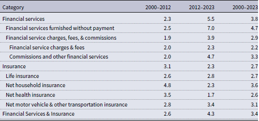
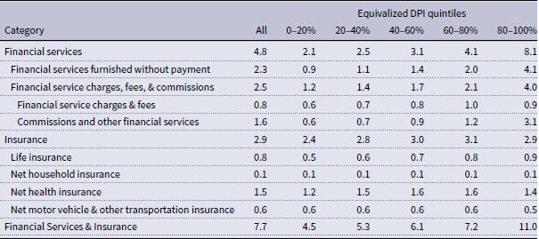
The convergence stems from two primary factors: the rapid growth in financial services prices and the compositional differences in expenditure across income groups. Financial services and insurance prices grew at an exceptional pace during our sample period – 3.4% annually, faster than most major expenditure categories. Given the empirical importance of this group, we decompose the category into key components from NIPA Table 2.4.4U in Table A1. In the second half of the period (2012–2023), financial services (5.5% annually) grew significantly faster than insurance (2.3%). The growth in financial services was driven by large price increases in two categories which are in PCE but not in the CPI: “Financial services furnished without payment” (7.0%) and “Commissions and other financial services” (4.7%), an aggregation whose dominant component is “Portfolio management and investment advice services.”Footnote 15 In contrast, “Financial service charges fees”, which is also covered in the CE and CPI and includes explicit costs like checking and overdraft fees, grew at a much slower pace (2.3% annually). Distinct from the two categories with higher price growth, however, its expenditure shares are lower overall and vary much less across quintiles (see Table A2).
Unlike explicit fees, financial services furnished without payment include imputed services from financial intermediation—charges that banks and other financial institutions implicitly levy for services like payment processing, account maintenance, and credit provision. In the NIPAs, these imputed services are calculated based on the difference between interest received and paid by financial institutions, scaled by measures of financial activity and asset holdings.Footnote 16, Footnote 17
The other key component, portfolio management, is also closely linked to asset returns and fee rates.Footnote 18 When asset values appreciate due to market gains, portfolio managers earn higher dollar revenues by applying the same percentage-based fee to larger portfolio balances, reflecting higher prices for portfolio management services.
Accordingly, we distribute these financial expenditures (furnished without payment and portfolio management) proportionally to asset balances, rather than according to CE-defined out-of-pocket financial services spending, in contrast to Carloni (Reference Carloni2025). As a result, they have an outsized impact on PCE inflation among high-expenditure households, as also shown in Martin et al. (Reference Martin, Matsumoto, Garner and Curtin2024). If, instead, we allocate these financial services proportionally to out-of-pocket financial services, our results follow a qualitative pattern closer to Carloni (Reference Carloni2025) and the CPI-based literature.
2.4.2. Timeline of price changes
During our period, financial services prices rose initially due to higher fees and returns. They fell during the financial crash, and rebounded strongly afterwards as investors capitalized on low interest rates and asset returns surged from 2012–2020.Footnote 19 They continued to grow throughout the COVID era, despite intra-period volatility. Commercial banking prices initially increased alongside the loan expansion (2020–2021), and subsequently increased further as the Federal Reserve raised interest rates (2022–2023). Conversely, while initially portfolio management prices continued to grow with the market, they declined markedly in anticipation of rising interest rates in 2022.
2.4.3. Differential exposure across income groups
Higher-income households are disproportionately exposed to financial services inflation for several reasons. They maintain larger and more complex portfolios of financial assets, engage in more frequent financial transactions, and utilize sophisticated banking services. They are also more likely to hold assets that generate imputed financial services, such as checking accounts, money market funds, and brokerage accounts. As Table 1 shows, financial services and insurance represent more than twice the expenditure share for top-quintile households (11.0%) compared to bottom-quintile households (4.5%).Footnote 20
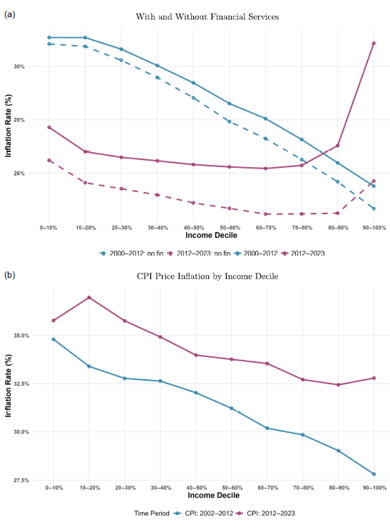
Accordingly, we can explore the impact of removing financial services and insurance from PCE. Figure A1 (panel a) repeats Figure 1b, but with additional (dashed) lines demonstrating the impact by period. For 2000–2012, there’s virtually no impact, as the price of financial services did not differ markedly from overall PCE. However, in the more recent period, removing financial services significantly reduces the inflation burden for the top two deciles, who are the most exposed due to their high level of assets. This is logically consistent with the fact that households in the top quintile of the income distribution also hold 75% of all financial assets.Footnote 21 Yet, the overall shape remains the same, much flatter than the first period, highlighting that the change in trend over the period is not solely driven by the contribution of financial services. Moreover, if this exercise is done with CPI (panel b) we also see a significant flattening in the latter half of the period.
2.5. Real income growth implications
The implications of these findings extend beyond inflation measurement to our understanding of real income dynamics across the distribution.
Figure 3a compares real DPI growth across quintiles, deflating nominal income growth using either group-specific IS-PCEPX (light bars) or the aggregate PCEPX (as produced by BEA, dark bars).
Measuring “Real” income growth (2000–2023).
Note: This figure compares real growth under different definitions of income and price indices. Panel (a) compares growth in Disposable Personal Income (DPI) by quintile, deflated alternatively by IS-PCEPX (light columns) and PCEPX (dark columns). The height of each column represents cumulative growth in income over the period. The y-axis is truncated at 100% at the bottom. Quintiles are based on equivalized DPI. Panel (b) shows the differences in income growth, deriving from income definitions and price indices, using four lines: (1) PI-PCEX: growth in personal income (PI), deflated by PCEPX [red solid], (2) PI-CPI: growth in PI, deflated by the Consumer Price Index (CPI) [red-dashed], (3) AMI-PCEPX: growth in Adjusted Money Income (AMI), deflated by PCEPX [blue solid], and (4) AMI-CPI: growth in AMI, deflated by CPI. AMI is a subset of PI, similar to the definition of money income used by the Census Bureau, but scaled to national accounts totals. It excludes health care, financial imputations, and some transfers included in PI.

Using income group-specific deflators has a modest impact on the real income growth gradient. While the bottom quintile experiences slightly higher growth than the top under the aggregate deflator, this pattern is reversed for the group-specific deflator. However, the magnitudes are very small. Over the full 2000–2023 period, the gap in real income growth between the bottom and top quintiles is approximately 1–2 percentage points using either approach, with group-specific deflators showing a slightly larger gap than when using the aggregate deflator.
More importantly, the convergence in inflation experiences over time means this flattening effect has grown stronger in recent years. During the latter part of our sample period, differential inflation has become less crucial for understanding real income growth patterns across the distribution.
Figure 3b extends this analysis by comparing different combinations of income measures and price indices over 2005–2023. The figure shows that the choice between PI and adjusted money income (AMI), a more narrowly defined measure similar to Census Bureau definitions,Footnote 22 matters more for real growth patterns than the choice between IS-PCEPX and group-specific CPI deflators.Footnote 23 This suggests that income, which includes transfers and in-kind benefits, is crucial for understanding differences in growth.
The results demonstrate that while PCE inflation inequality is present and measurable, its contribution to overall income inequality trends has been smaller and more dynamic than what has been documented using the CPI. For our available time period, the story is not one of persistent, large disadvantages for low-income households, but rather of modest differences that have been converging over time as the structure of the economy and patterns of price growth have evolved.
3. Conclusion
Using the first income-stratified PCE price indices consistent with national accounts, we find inflation inequality has recently been converging rather than persisting. While the bottom decile experienced 0.3 percentage points higher annual inflation than the top decile during 2000–2012, this pattern reversed during 2012–2023. Leveraging a national accounts approach, we find annual gaps of 0.13 percentage points, compared with 0.29 percentage points using the CPI (Jaravel, Reference Jaravel2026).
The choice of price index (PCE vs. CPI) can fundamentally alter conclusions about distributional inflation patterns. The comprehensive nature of PCE captures expenditures at the national level, including those not directly made by households. Accordingly, we find a convergence in inflation, which stands in contrast to results from CPI-based studies. The primary driver of this pattern is rapid inflation in financial services and insurance, which disproportionately affects higher-income households due to their greater exposure to these services. The inclusion of financial services, however, is vital for understanding consumption for top income households, especially as those with highest incomes typically also have the highest wealth.
Our analysis faces several limitations. As with other research exercises tying income to expenditures, the integration of BEA income distributions with BLS expenditure distributions requires harmonizing different data sources, potentially introducing measurement error. However, in order to create indices that represent national accounts (broad concepts), a degree of imputation is necessary. Our 2000-2023 period may not capture longer-term patterns, but allows us to focus on the more recent years, and thus the trend.
Additionally, as discussed in Section 1, our analysis captures differences in PCE inflation by income group by using group-specific weights to re-aggregate the same set of elementary indexes. That means for an elementary category like new motor vehicles, the results do not reflect any inflation differences arising from potentially different spending patterns across different vehicle types or different prices paid for the same vehicle. Jaravel (Reference Jaravel2018), using barcode scanner data for food, beverages, and other consumer packaged goods, finds that starting from a constant set of (relatively broad) elementary aggregates rather than individual barcodes can understate inflation gaps between the bottom and top of the income distribution. Inflation inequality studies based on the full CPI, including Jaravel (Reference Jaravel2026) and Klick and Stockburger (Reference Klick and Stockburger2024), as well as our study, are potentially subject to this “aggregation bias.”Footnote 24 Given that we find a similar Q1–Q5 inflation gap of 0.29 if we use PCE data to calculate income-quintile price indexes with comparable ranking, formula and scope to Jaravel (Reference Jaravel2026), we are reassured that the issue of aggregation bias does not differentially affect group PCE price indexes relative to group CPIs.Footnote 25
The integration of income and expenditure distributions within national accounts provides a template for extending distributional analysis to other economic measures. The prominence of financial services inflation highlights the need for better understanding how the financial sector affects household experiences across the income distribution. Our methodology enables inflation inequality analysis using the Federal Reserve’s preferred price index, potentially informing research on monetary policy and distributional effects.
Competing interests
The author(s) declare none.
A. Appendix
Financial services & insurance: decomposed inflation, 2000–2023 all values are expressed as percentages

Note: This table shows the annualized inflation (as calculated by the authors) for each selected Personal Consumption Expenditure (PCE) item from NIPA Table 2.4.4U, by period. The category “Commissions and other financial services” is an aggregation of lines 260:“Securities commissions”, 268: “Portfolio management and investment advice services”, and 269:“Trust, fiduciary, and custody activities.”.
Financial services & insurance expenditure shares, 2000–2023 all values are expressed as percentages

Note: This table shows the expenditure shares of select Personal Consumption Expenditure (PCE) items, as a percentage of total PCE, both overall and by quintile as ranked on equivalized Disposable Personal Income (DPI). The category “Commissions and other financial services” is an aggregation of lines 260:“Securities commissions”, 268: “Portfolio management and investment advice services”, and 269:“Trust, fiduciary, and custody activities.”.
PCE categories out-of-scope* to CPI

Notes: Following McCully et al. (Reference McCully, Moyer and Stewart2007), “out-of-scope” refers both to categories that are not included in the CPI (such as financial services furnished without payment), as well as categories that are included in the CPI, but have substantial definitional differences relative to PCE (such as physician services). “NIPA line” refers to the line number from NIPA Table 2.4.5U. For additional detail on CPI-PCE differences, see Blair (Reference Blair and Blair2015).
CPI categories out-of-scope* to PCE

Notes: Following McCully et al. (Reference McCully, Moyer and Stewart2007), “out-of-scope” refers both to categories that are not included in PCE (such as state automobile registrations), as well as categories that are included in PCE, but have substantial definitional differences relative to CPI (such as physicians’ services). “NIPA line” refers to the line number from NIPA Table 2.4.5U. The shares are the relative importance in December 2022 using 2021 weights (U.S. Bureau of Labor Statistics, 2022). For additional detail on CPI-PCE differences, see Blair (Reference Blair and Blair2015).
IS-PCEPX-CPI comparison for goods and services (2002–2023) all values are expressed as percentages

Note: This table compares the IS-PCEPX and Consumer Price Index (CPI) both overall and for goods and services separately. The columns show inflation for the full population and the stratification by income quintile. Income quintiles are ranked on equivalized Disposable Personal Income (DPI). Q1–Q5 refers to the gap between the bottom and the top quintile. The Personal Consumption Expenditure (PCE) Price index for All is the official BEA measure, and quintiles are constructed using equivalized DPI. The CPI by quintile estimates are constructed using the replication files from (Jaravel, Reference Jaravel2026), and quintiles are constructed using equivalized Consumer Expenditure before-tax income.
Cumulative inflation by period: Alternative definitions.
Note: This figure accompanies Figure 1b by repeating cumulative inflation by decile for two periods (blue = 2000–2012; purple = 2012–2023). In panel (a), additional dashed lines are added for each period to represent the cumulative inflation without the inclusion of financial services. In panel (b) inflation is computed using Consumer Price Index (CPI) data from available microdata files in Jaravel (Reference Jaravel2026).