1 Introduction
The ability to attain quantitatively reliable predictions of fluidized bed behaviour is highly dependent on the accuracy of the fluid–particle drag force, since in fluidized beds, the buoyant weight of particles is principally balanced by the drag force exerted by the flowing fluid. In numerical studies of industrial-scale systems, the interactions between fluid and particles cannot be fully resolved at the scale of the particle’s surface due to limitations in computational power. Instead, in these large-scale simulations, the fluid computational grid size is larger than a particle diameter, and so constitutive relations for the fluid–particle drag force are necessary. The accuracy of these drag models at the particle-scale level is vital in order to achieve quantitative precision in the study of fluidized beds. Despite this fact, there are a number of limitations to the drag models that are commonly employed in the literature. While a number of recent studies (Xu, Ge & Li Reference Xu, Ge and Li2007; Wang, Liu & You Reference Wang, Liu and You2011; Zhou et al. Reference Zhou, Xiong, Wang, Wang, Ren and Ge2014) have elucidated the effect of the magnitude and direction of inhomogeneities in the particle configuration on the drag, these studies have not resulted in a generalized inhomogeneity-dependent drag model that can be applied as a constitutive closure to larger-scale fluidization simulations. Thus, the current work primarily addresses the need for the development of such a drag relation that accounts for inhomogeneities in the distribution of particles.
Prior drag models that have been employed in large-scale simulations of fluidized beds are typically based on either the sedimentation of particles (Richardson & Zaki Reference Richardson and Zaki1954; Wen & Yu Reference Wen and Yu1966; Garside & Al-Dibouni Reference Garside and Al-Dibouni1977) or fixed particle beds (Hill, Koch & Ladd Reference Hill, Koch and Ladd2001; van der Hoef, Beetstra & Kuipers Reference van der Hoef, Beetstra and Kuipers2005; Beetstra, van der Hoef & Kuipers Reference Beetstra, van der Hoef and Kuipers2007; Tenneti, Garg & Subramaniam Reference Tenneti, Garg and Subramaniam2011). Typically, these drag models are expressed in terms of a dimensionless drag force,
 $F$
, which is defined as:
 $$\begin{eqnarray}F={\displaystyle \frac{\boldsymbol{F}_{fp}\boldsymbol{\cdot }\boldsymbol{u}_{slip}}{\boldsymbol{F}_{d,Stokes}\boldsymbol{\cdot }\boldsymbol{u}_{slip}}},\end{eqnarray}$$
where
 $\boldsymbol{F}_{fp}$
is the total fluid–particle interaction force per particle minus the generalized buoyancy arising from the slowly varying stress field,
 $\boldsymbol{u}_{slip}$
is the slip velocity, which is the difference between the fluid velocity,
 $\boldsymbol{u}_{f}$
, and the particle velocity,
 $\boldsymbol{v}_{p}$
, and the Stokes drag relation on a single spherical particle at infinite dilution in a viscous fluid is given by:
 $$\begin{eqnarray}\boldsymbol{F}_{d,Stokes}=3\unicode[STIX]{x03C0}\unicode[STIX]{x1D707}_{f}d_{p}\boldsymbol{u}_{slip},\end{eqnarray}$$
where
 $d_{p}$
is diameter of the particle and
 $\unicode[STIX]{x1D707}_{f}$
is the dynamic fluid viscosity. These drag models are typically expressed as functions of the particle volume fraction,
 $\unicode[STIX]{x1D719}$
, and Reynolds number (Re), which is defined as:
 $$\begin{eqnarray}Re={\displaystyle \frac{\unicode[STIX]{x1D70C}_{f}(1-\unicode[STIX]{x1D719})|\boldsymbol{u}_{slip}|d_{p}}{\unicode[STIX]{x1D707}_{f}}},\end{eqnarray}$$
where
 $\unicode[STIX]{x1D70C}_{f}$
is the fluid density. Recently, the Rubinstein, Derksen & Sundaresan (Reference Rubinstein, Derksen and Sundaresan2016) model expanded upon these traditional drag relations by accounting for the effects of particle inertia through the Stokes number (
 $St$
), which is the ratio of the particle relaxation time to the fluid relaxation time, and is defined as:
 $$\begin{eqnarray}St={\displaystyle \frac{\unicode[STIX]{x1D70C}_{p}(1-\unicode[STIX]{x1D719})|\boldsymbol{u}_{slip}|d_{p}}{18\unicode[STIX]{x1D707}_{f}}}.\end{eqnarray}$$
While the Rubinstein et al. (Reference Rubinstein, Derksen and Sundaresan2016) drag model provides a significant improvement over prior drag relations in its ability to implicitly account for the effects of particle translation and rotation through
 $St$
, one key limitation that persists is that this drag model is only applicable to random, homogeneous distributions of particles. This constitutive relation relies on the key assumption that the distribution of particles is homogeneous at the scale at which the model is applied. However, the effect of the extent of inhomogeneities on the drag force has been found to be significant, even at the small scale of several particle diameters (Kriebitzsch, van der Hoef & Kuipers Reference Kriebitzsch, van der Hoef and Kuipers2013; Zhou et al.
Reference Zhou, Xiong, Wang, Wang, Ren and Ge2014). Thus, the goal of the current work is to develop a new drag model that is able to account for the effect of inhomogeneities.
The importance of inhomogeneities in the particle distribution on the behaviour of fluidized beds has been demonstrated by a number of studies. In fluidized bed simulations based on the two-fluid model (TFM), achieving grid size convergence with traditional drag closures has proven to be very difficult, even at grid sizes as small as 10
 $d_{p}$
, due to the presence of heterogeneous structures (Agrawal et al.
Reference Agrawal, Loezos, Syamlal and Sundaresan2001; Igci et al.
Reference Igci, Andrews, Sundaresan, Pannala and O’Brien2008; Li et al.
Reference Li, Gel, Pannala, Shahnam and Syamlal2014). In particular, for Geldart Group A particles, typical fine-grid TFM simulations are unable to predict the behaviour that is observed experimentally (Lu, Wang & Li Reference Lu, Wang and Li2009; Wang, van der Hoef & Kuipers Reference Wang, van der Hoef and Kuipers2009; Cloete, Johansen & Amini Reference Cloete, Johansen and Amini2015; Liu et al.
Reference Liu, Zhu, Geng, Yao, Zhan and Xu2015). These shortcomings are especially pronounced in high-velocity systems, where homogeneous drag models are unable to resolve all of the mesoscale structures (Hong et al.
Reference Hong, Chen, Wang and Li2016). While the effects of particle cohesion and fluid turbulence could have contributed to the observed differences between the TFM simulations and experiments of fluidized beds with Geldart Group A particles, prior studies, like that of Wang et al. (Reference Wang, van der Hoef and Kuipers2009), have found that, due to the significance of inhomogeneities at relatively small length scales, a sufficiently fine-grid size is needed in order to accurately simulate the flow characteristics using TFM. Thus, failing to account for particle structures significantly affects the computed fluid–particle drag. In the current work, by focusing on low-Re systems with non-cohesive particles, we singularly study the effects of inhomogeneities. This choice of fluidized bed simulations therefore provides a direct method to probe the specific effects of inhomogeneities on the drag force.
One of the key measures that has been used in prior studies to quantify the extent of inhomogeneities is the solid volume fraction gradient,
 $\unicode[STIX]{x1D735}\unicode[STIX]{x1D719}$
. This quantity,
 $\unicode[STIX]{x1D735}\unicode[STIX]{x1D719}$
, has been found to correlate with the grid size required to achieve grid convergence (Fullmer & Hrenya Reference Fullmer and Hrenya2016). Furthermore, in fixed particle systems with simple linear variations in
 $\unicode[STIX]{x1D719}$
, it has been demonstrated that the drag is affected by both the magnitude of
 $\unicode[STIX]{x1D735}\unicode[STIX]{x1D719}$
and the angle between
 $\boldsymbol{u}_{slip}$
and
 $\unicode[STIX]{x1D735}\unicode[STIX]{x1D719}$
(Zhou et al.
Reference Zhou, Xiong, Wang, Wang, Ren and Ge2014; Li et al.
Reference Li, Wang, Rogers, Zhou and Ge2017). Larger magnitudes of
 $\unicode[STIX]{x1D735}\unicode[STIX]{x1D719}$
lead to larger changes in the drag. In terms of the directional effect, when
 $\unicode[STIX]{x1D735}\unicode[STIX]{x1D719}$
is aligned with the slip velocity, the fluid flow has to move through an area where there is a high concentration of particles, causing there to be an increase in the drag. On the other hand, when
 $\unicode[STIX]{x1D735}\unicode[STIX]{x1D719}$
is perpendicular to the slip velocity, the fluid flow can easily by-pass the areas with high concentration of particles, leading to a reduction in the drag. Thus, the drag is maximized when
 $\boldsymbol{u}_{slip}$
is parallel to
 $\unicode[STIX]{x1D735}\unicode[STIX]{x1D719}$
, and is minimized when
 $\boldsymbol{u}_{slip}$
is perpendicular to
 $\unicode[STIX]{x1D735}\unicode[STIX]{x1D719}$
(Zhou et al.
Reference Zhou, Xiong, Wang, Wang, Ren and Ge2014; Li et al.
Reference Li, Wang, Rogers, Zhou and Ge2017). In demonstrating the importance of the
 $\unicode[STIX]{x1D735}\unicode[STIX]{x1D719}$
measure, these studies have further emphasized how significant inhomogeneities are to the behaviour of fluidized beds.
While there have been some prior attempts to correct the homogeneous drag models with additional terms that are computed using detailed particle distribution information (Xu et al. Reference Xu, Ge and Li2007; Wang et al. Reference Wang, Liu and You2011), prior studies have not arrived at a drag model that can both account for the effect of inhomogeneities and be easily applied to TFM and computational fluid dynamics-discrete element method (CFD-DEM) larger-scale simulations. The goal of the current study is to therefore take the insights gained from these prior studies, and use them to derive a new drag constitutive relation that not only accounts for the effect of particle distribution inhomogeneities, but is also applicable as a closure to a variety of larger-scale simulations. Towards this goal, lattice Boltzmann method (LBM) simulations of fluidized beds are performed. Using the detailed flow and particle configuration data obtained from these simulations, the fluid–particle drag is found to depend on a subgrid-scale measure for the extent of inhomogeneities. Models to estimate these subgrid quantities are developed that are based on a scale-similarity approach, which was originally derived for single-phase turbulence (Germano et al. Reference Germano, Piomelli, Moin and Cabot1991) and later adapted to applications in multiphase flow (Parmentier, Simonin & Delsart Reference Parmentier, Simonin and Delsart2012; Ozel, Fede & Simonin Reference Ozel, Fede and Simonin2013). By accounting for the effect of inhomogeneities, these newly derived constitutive relations for the fluid–particle drag force provide a significant improvement over prior models that assumed a random, homogeneous distribution of particles.
In § 2, we describe prior drag modelling attempts, our LBM simulation scheme, and the filtering method used to analyse the results. In § 3, we provide the simulation results from this study, as well as the development of our new drag models that account for inhomogeneities in the distribution of particles in low-Re systems. In § 4, we provide some concluding remarks on the overall findings of this study.
2 Methodology
2.1 Prior drag modelling
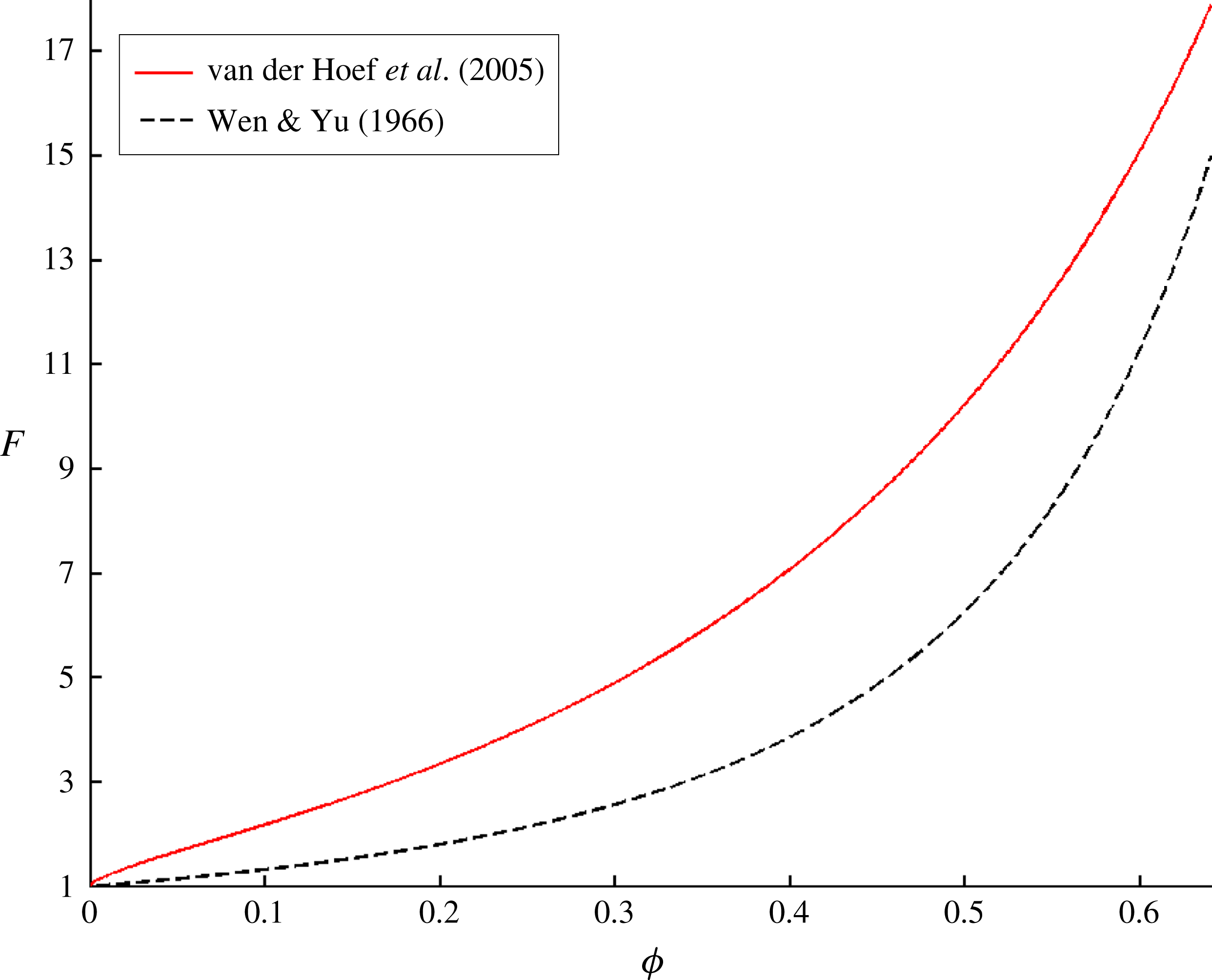
In figure 1, we see that in the low-Re regime, the fixed bed dimensionless drag (van der Hoef et al.
Reference van der Hoef, Beetstra and Kuipers2005) is significantly greater than the particle sedimentation drag (Wen & Yu Reference Wen and Yu1966) over the entire range of
 $\unicode[STIX]{x1D719}$
. While the granular temperature has been shown to have a significant effect on the drag in dynamic fluidized beds at larger Re (Tang, Peters & Kuipers Reference Tang, Peters and Kuipers2016), this quantity has a small effect in the low-Re regime. Instead, this large difference in the drag relations, which was identified in our prior work (Rubinstein et al.
Reference Rubinstein, Derksen and Sundaresan2016), is attributed to
 $St$
(1.4). In the low-Re regime, the fixed bed drag can be thought of as the high-
 $St$
-limit drag, while the particle sedimentation drag can be thought of as the low-
 $St$
-limit drag. Furthermore, in this prior work, we proposed a new
 $St$
-dependent drag model that was able to bridge the transition from the low-
 $St$
limit to the high-
 $St$
limit. This drag model has the following form:
 $$\begin{eqnarray}F(\unicode[STIX]{x1D719},St)=\unicode[STIX]{x1D6FC}(St_{mod})F_{vdH}(\unicode[STIX]{x1D719})+(1-\unicode[STIX]{x1D6FC}(St_{mod}))(1-\unicode[STIX]{x1D719})^{-(n(\unicode[STIX]{x1D719})-2)},\end{eqnarray}$$
where the high-
 $St$
-limit drag is given by the van der Hoef et al. (Reference van der Hoef, Beetstra and Kuipers2005) curve:
 $$\begin{eqnarray}F_{vdH}(\unicode[STIX]{x1D719})={\displaystyle \frac{10\unicode[STIX]{x1D719}}{1-\unicode[STIX]{x1D719}}}+(1-\unicode[STIX]{x1D719})^{3}(1+1.5\sqrt{\unicode[STIX]{x1D719}}),\end{eqnarray}$$
and the low-
 $St$
-limit drag is given by:
 $$\begin{eqnarray}F_{low\,St}(\unicode[STIX]{x1D719})=(1-\unicode[STIX]{x1D719})^{-(n(\unicode[STIX]{x1D719})-2)},\end{eqnarray}$$
with
 $n(\unicode[STIX]{x1D719})=6.2-2.5\unicode[STIX]{x1D719}$
. The parameter
 $\unicode[STIX]{x1D6FC}$
, which describes the transition from the low-
 $St$
limit to the high-
 $St$
limit, is given by:
 $$\begin{eqnarray}\unicode[STIX]{x1D6FC}(St_{mod})={\displaystyle \frac{1}{2}}\left(1+{\displaystyle \frac{St_{mod}-10}{St_{mod}+10}}\right),\end{eqnarray}$$
where the modified Stokes number,
 $St_{mod}$
, is defined as:
 $$\begin{eqnarray}St_{mod}={\displaystyle \frac{St}{(1-\unicode[STIX]{x1D719})^{2}}}.\end{eqnarray}$$
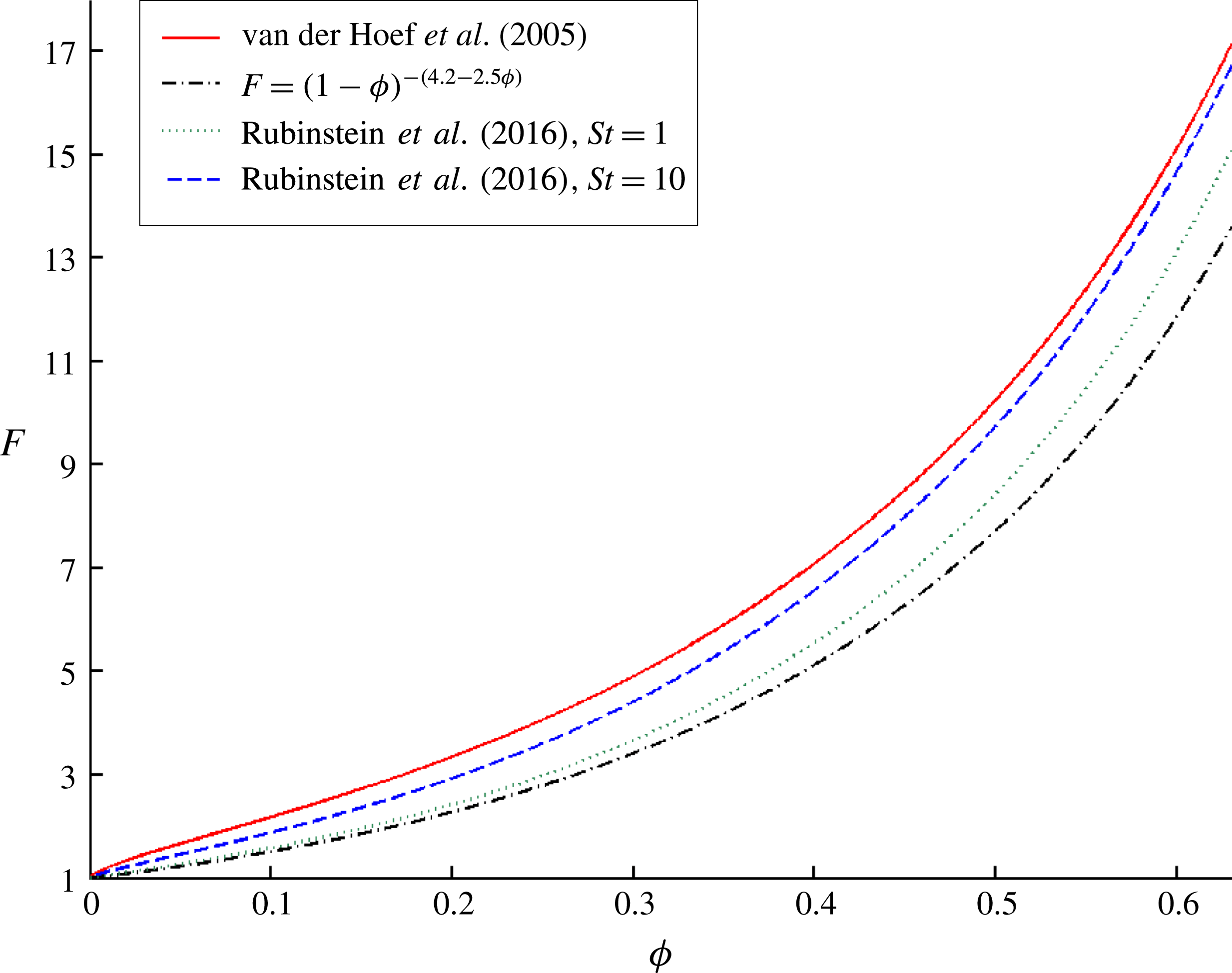
This new
 $St$
-dependent drag model is shown in figure 2.
The low-Re dimensionless drag force,
 $F$
, is plotted as a function of particle volume fraction,
 $\unicode[STIX]{x1D719}$
, for the both the van der Hoef et al. (Reference van der Hoef, Beetstra and Kuipers2005) model for fixed particle beds (high-
 $St$
limit) and the Wen & Yu (Reference Wen and Yu1966) model for sedimenting particle beds (low-
 $St$
limit).

The Rubinstein et al. (Reference Rubinstein, Derksen and Sundaresan2016) drag model, which accounts for the effects of
 $St$
, is plotted over a range of
 $\unicode[STIX]{x1D719}$
and
 $St$
. The van der Hoef et al. (Reference van der Hoef, Beetstra and Kuipers2005) curve represents the high-
 $St$
limit of this model, while the
 $F=(1-\unicode[STIX]{x1D719})^{-(4.2-2.5\unicode[STIX]{x1D719})}$
curve represents the low-
 $St$
limit of this model.

2.2 LBM scheme
In this study, LBM simulations of fluidized beds are employed in order to develop a new drag model that can account for the effect of inhomogeneities. In LBM, the fluid flow is represented by the movement of fluid parcels along a three-dimensional lattice of nodes. These fluid dynamics are governed by the Boltzmann equation, which is discretized in both time and space. In the low-Mach-number limit, these discretized Boltzmann equations converge to the incompressible Navier–Stokes equations when averaged over a sufficiently large volume (Chen & Doolen Reference Chen and Doolen1998). The LBM scheme employed in this study is based on a slight variant of the widely used LBGK scheme (Qian, D’Humieres & Lallemand Reference Qian, D’Humieres and Lallemand1992). This scheme, which is used to solve for the evolution of the fluid density and momentum distributions, is described in more detail by Somers (Reference Somers1993) and Eggels & Somers (Reference Eggels and Somers1995).
The interactions between the solid particles and fluid, which were first studied using LBM by Ladd (Reference Ladd1994), are resolved using a technique similar to the immersed boundary method (Goldstein, Handler & Sirovich Reference Goldstein, Handler and Sirovich1993; Derksen & Van den Akker Reference Derksen and Van den Akker1999; ten Cate et al. Reference ten Cate, Nieuwstad, Derksen and van den Akker2002). This forcing mechanism ensures that the no-slip boundary condition is satisfied by imposing additional forces on the fluid along the surface of the solid particle. The net force and torque that the fluid exerts on a solid particle is then computed by summing over these local surface forces. An additional particle–particle lubrication force, which accounts for unresolved, subgrid flow contributions when the gap between two particles is smaller than the lattice grid size, is introduced into the scheme (Kim & Karilla Reference Kim and Karilla1991; Nguyen & Ladd Reference Nguyen and Ladd2002). Furthermore, in order to computationally facilitate collisions between particles, each of the solid particles is given a small degree of softness. Particle–particle collisions still effectively resemble hard sphere collisions, as the maximum overlap distance is approximately 0.001 particle diameters. At each time step, the velocity and position of the particles are updated by using the total force and torque acting on each particle. Further details of the LBM numerical scheme used in this study can be found in Derksen & Sundaresan (Reference Derksen and Sundaresan2007) and Rubinstein et al. (Reference Rubinstein, Derksen and Sundaresan2016).
In the current study, fluidized beds with spherical monodisperse particles are simulated in a cubic domain with fully periodic boundary conditions in all dimensions. In this periodic system, a body force is applied to all of the fluid and particles in order to drive flow in the system and balance the net weight of the fluid and particles (Derksen & Sundaresan Reference Derksen and Sundaresan2007). Since the lattice units are dimensionless, for simplicity, the lattice spacing,
 $\unicode[STIX]{x1D6E5}$
, and the time step are taken to be
 $1$
. The parameters that define a given system are: the particle diameter,
 $d_{p}$
, the fluid kinematic viscosity,
 $\unicode[STIX]{x1D708}_{f}$
, the particle-to-fluid density ratio,
 $\unicode[STIX]{x1D70C}_{p}/\unicode[STIX]{x1D70C}_{f}$
, the strength of the applied external body force,
 $f_{ext}$
, the total number of particles,
 $N$
, and the dimensions of the lattice,
 $n_{x}$
,
 $n_{y}$
, and
 $n_{z}$
. For the current study,
 $d_{p}=12$
and
 $\unicode[STIX]{x1D708}_{f}=0.1$
. While larger values of
 $d_{p}$
would correspond to higher resolutions of the fluid flow profile, the chosen combination of values was previously shown to provide a sufficient level of resolution in order to achieve convergence in the flow behaviour in the low-Re regime (Rubinstein et al.
Reference Rubinstein, Derksen and Sundaresan2016). Furthermore, in order to obtain a sufficiently large domain where inhomogeneous structures are able to form, we choose:
 $n_{x}=n_{y}=n_{z}=12d_{p}$
. The domain-averaged volume fraction,
 $\langle \unicode[STIX]{x1D719}\rangle$
, is defined as:
 $$\begin{eqnarray}\langle \unicode[STIX]{x1D719}\rangle ={\displaystyle \frac{N\left({\displaystyle \frac{\unicode[STIX]{x03C0}}{6}}d_{p}^{3}\right)}{n_{x}n_{y}n_{z}}}.\end{eqnarray}$$
 $St$
cannot be set a priori, and so it is, instead, computed from the results of the simulation. In this study,
 $f_{ext}$
,
 $\unicode[STIX]{x1D70C}_{p}/\unicode[STIX]{x1D70C}_{f}$
, and
 $\langle \unicode[STIX]{x1D719}\rangle$
are varied so that large ranges of
 $St$
and inhomogeneous structures are sampled. In particular, since the study is focused on the low-Re regime, a given simulation is defined by the following pair of parameters:
 $\unicode[STIX]{x1D70C}_{p}/\unicode[STIX]{x1D70C}_{f}$
and
 $\langle \unicode[STIX]{x1D719}\rangle$
.
In this study, using the insights developed in our prior work (Rubinstein et al.
Reference Rubinstein, Derksen and Sundaresan2016), we utilized two additional types of LBM simulations: high-
 $St$
-limit and low-
 $St$
-limit beds. Since particles are slow to adapt to the surrounding fluid in the high-
 $St$
regime, in the high-
 $St$
limit simulations, the fluid flow establishes an equilibrium around a bed of fixed particles, with the particle translational and rotational velocities held fixed at
 $0$
. Since particles adapt very quickly to the surrounding fluid in the low-
 $St$
regime, in the low-
 $St$
-limit simulations, the fluid flow and particle velocities are allowed to evolve until the net force and torque on each particle is
 $0$
, while the particles are held fixed in place. Further details of the high-
 $St$
-limit and low-
 $St$
-limit simulations are presented in Rubinstein et al. (Reference Rubinstein, Derksen and Sundaresan2016).
2.3 Analysing LBM results: filtering procedure
The goal of the current study is to analyse the effect of inhomogeneous structures on the fluid–particle drag. While our prior analysis simply looked to compute domain-averaged LBM quantities, such an approach would be insufficient for resolving these different structures. Thus, in the current study, a filtering technique is employed, in which the LBM simulation results are analysed over a range of length scales. In this method, first of all, the Lagrangian particle variables are mapped onto an Eulerian grid with a base cell size of
 $\unicode[STIX]{x1D6E5}_{b}=1d_{p}$
using a Gaussian-type mapping function (Pepiot & Desjardins Reference Pepiot and Desjardins2012),
 $g(s)$
, which is given by:
 $$\begin{eqnarray}g(s)=\left\{\begin{array}{@{}ll@{}}{\displaystyle \frac{1}{4}}s^{4}-{\displaystyle \frac{5}{8}}s^{2}+{\displaystyle \frac{115}{192}},\quad & s\leqslant 0.5\\ -{\displaystyle \frac{1}{6}}s^{4}+{\displaystyle \frac{5}{6}}s^{3}-{\displaystyle \frac{5}{4}}s^{2}+{\displaystyle \frac{5}{24}}s+{\displaystyle \frac{55}{96}},\quad & 0.5<s\leqslant 1.5\\ {\displaystyle \frac{(2.5-s)^{4}}{24}},\quad & 1.5<s\leqslant 2.5\\ 0,\quad & s>2.5.\end{array}\right.\end{eqnarray}$$
In (2.7),
 $s$
is the distance between the particle centre and grid centre, normalized by the Eulerian grid size,
 $\unicode[STIX]{x1D6E5}_{b}$
. The fully resolved fluid lattice grid variables are then coarsened, via phase Favre averaging, to the
 $\unicode[STIX]{x1D6E5}_{b}=1d_{p}$
Eulerian grid using the mapping function in (2.7). The size of the base Eulerian grid is chosen to be
 $1d_{p}$
, since below this length scale, the fluctuations in the structures are too fine to effectively model. At this base grid size, the particle volume fraction, fluid velocity, particle velocity, and fluid–particle interaction force per unit volume are denoted as
 $\unicode[STIX]{x1D719}$
,
 $\boldsymbol{u}_{f}$
,
 $\boldsymbol{v}_{p}$
, and
 $\boldsymbol{f}_{fp}$
, respectively. Once all of these variables have been computed over this
 $1d_{p}$
Eulerian grid, the structures in each simulation system are studied over a range of length scales by defining a filter size,
 $\unicode[STIX]{x1D6E5}_{f}$
, which is greater than or equal to the base grid size,
 $\unicode[STIX]{x1D6E5}_{b}$
. Each of these variables is then filtered by performing either simple volume-averaging (
 $\unicode[STIX]{x1D719}$
,
 $\boldsymbol{f}_{fp}$
) or Favre averaging (
 $\boldsymbol{u}_{f}$
,
 $\boldsymbol{v}_{p}$
). These filtered variables are denoted as
 $\overline{\unicode[STIX]{x1D719}}$
,
 $\tilde{\boldsymbol{u}}_{f}$
,
 $\tilde{\boldsymbol{v}}_{p}$
, and
 $\overline{\boldsymbol{f}}_{fp}$
, and are computed as follows:
 $$\begin{eqnarray}\displaystyle & \displaystyle \overline{\unicode[STIX]{x1D719}}={\displaystyle \frac{\displaystyle \mathop{\sum }_{i}V_{cell,i}\unicode[STIX]{x1D719}_{i}}{\displaystyle \mathop{\sum }_{i}V_{cell,i}}}, & \displaystyle\end{eqnarray}$$
 $$\begin{eqnarray}\displaystyle & \displaystyle \tilde{u} _{f,j}={\displaystyle \frac{\displaystyle \mathop{\sum }_{i}V_{cell,i}(1-\unicode[STIX]{x1D719}_{i})u_{f,ij}}{\displaystyle \mathop{\sum }_{i}V_{cell,i}(1-\unicode[STIX]{x1D719}_{i})}}, & \displaystyle\end{eqnarray}$$
 $$\begin{eqnarray}\displaystyle & \displaystyle \tilde{v}_{p,j}={\displaystyle \frac{\displaystyle \mathop{\sum }_{i}V_{cell,i}\unicode[STIX]{x1D719}_{i}v_{p,ij}}{\displaystyle \mathop{\sum }_{i}V_{cell,i}\unicode[STIX]{x1D719}_{i}}}, & \displaystyle\end{eqnarray}$$
 $$\begin{eqnarray}\displaystyle & \displaystyle \overline{f}_{fp,j}={\displaystyle \frac{\displaystyle \mathop{\sum }_{i}V_{cell,i}f_{fp,ij}}{\displaystyle \mathop{\sum }_{i}V_{cell,i}}}, & \displaystyle\end{eqnarray}$$
where each of these sums is performed over all of the base grid cells that are contained within a particular filter cell,
 $V_{cell,i}$
is the volume of the
 $i\text{th}$
base grid cell, and the index
 $j$
is used to denote the
 $x$
,
 $y$
, and
 $z$
components. By using this filtering technique, the effect of inhomogeneities on the flow behaviour is studied over a range of length scales. To put our prior domain-averaged analysis into context, it is equivalent to performing a filtering analysis with
 $\unicode[STIX]{x1D6E5}_{f}=\unicode[STIX]{x1D6E5}_{b}=n_{x}$
.
3 Simulation results
3.1 Effect of inhomogeneities on drag
In order to demonstrate the significance of the effect of inhomogeneities on the drag force, we compared the drag in systems with random, homogeneous distributions of particles to those with inhomogeneous structures. Drawing upon our methodology in our prior work, our goal was to establish these inhomogeneity effects at the high- and low-
 $St$
limits. In doing so, we are able to isolate the effect of inhomogeneities from that of
 $St$
.
Random, homogeneous configurations of particles are obtained using a thermalization technique via DEM simulations, which is described in further detail by Rubinstein et al. (Reference Rubinstein, Derksen and Sundaresan2016). These random, homogeneous distributions are employed as the initial particle configurations in fluidized bed simulations. Inhomogeneous configurations of particles are then obtained by running fluidized bed simulations until a statistical steady state is reached. The statistical steady state is based on the time evolution of
 $\langle \boldsymbol{u}_{slip}\rangle$
. The final, inhomogeneous configuration is not correlated with the initial, homogeneous configuration, and so the inhomogeneity-dependent drag results obtained in this study are unaffected by the thermalization technique. In our study, we find that fluidized beds with different values of
 $\unicode[STIX]{x1D70C}_{p}/\unicode[STIX]{x1D70C}_{f}$
induce different extents of inhomogeneities, and so we investigate the properties of inhomogeneous configurations originating from fluidized beds with a range of
 $\unicode[STIX]{x1D70C}_{p}/\unicode[STIX]{x1D70C}_{f}$
values.
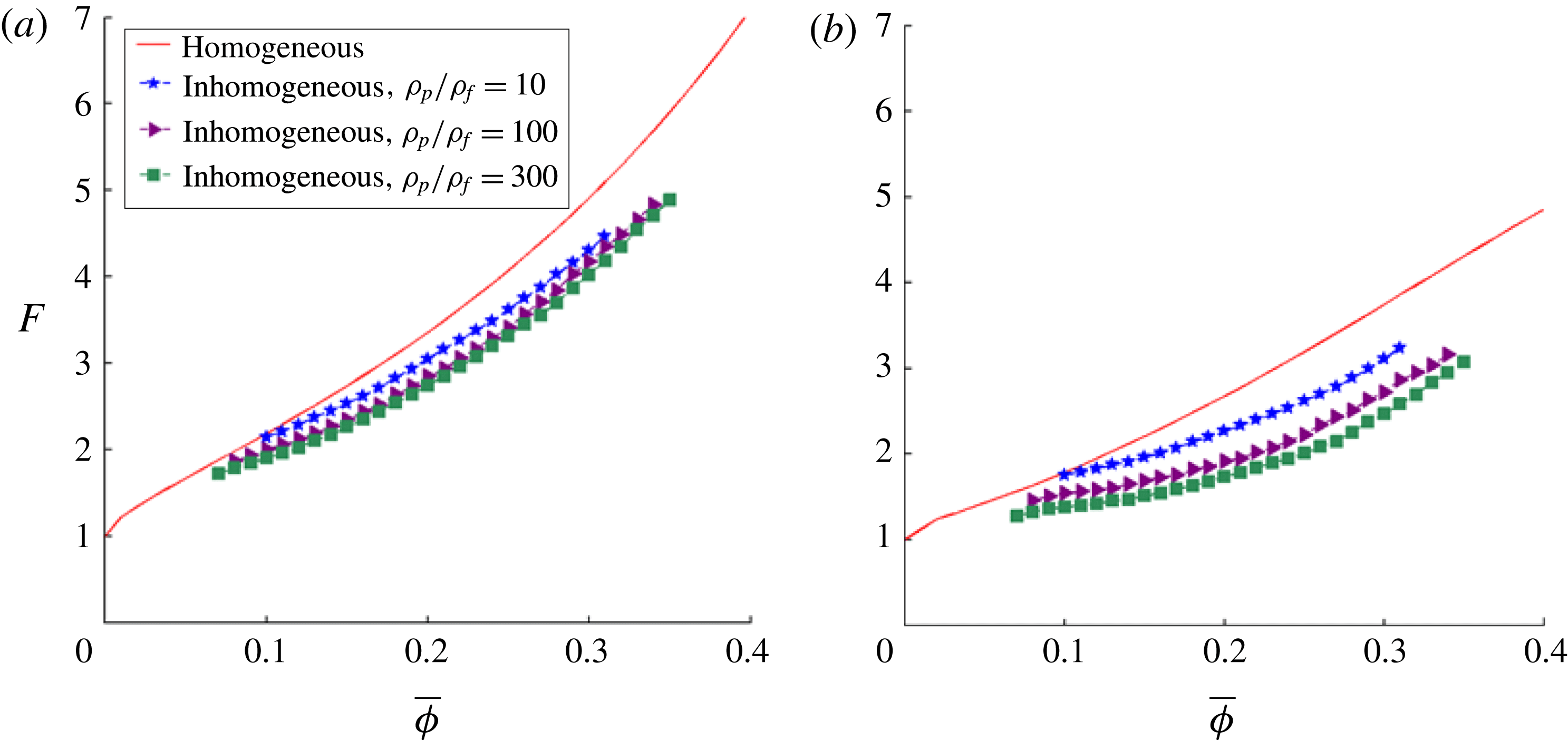
In figure 3, the random, homogeneous drag results are compared with the inhomogeneous drag results at the (a) high-
 $St$
limit and (b) low-
 $St$
limit. In this figure, the dimensionless drag force,
 $F$
, is plotted as a function of the filtered particle volume fraction,
 $\overline{\unicode[STIX]{x1D719}}$
. In terms of filtered quantities,
 $F$
is defined as:
 $$\begin{eqnarray}F={\displaystyle \frac{\overline{\boldsymbol{F}}_{fp}\boldsymbol{\cdot }\tilde{\boldsymbol{u}}_{slip}}{3\unicode[STIX]{x03C0}\unicode[STIX]{x1D707}_{f}d_{p}\tilde{\boldsymbol{u}}_{slip}\boldsymbol{\cdot }\tilde{\boldsymbol{u}}_{slip}}},\end{eqnarray}$$
where
 $\tilde{\boldsymbol{u}}_{slip}=\tilde{\boldsymbol{u}}_{f}-\tilde{\boldsymbol{v}}_{p}$
and
 $\overline{\boldsymbol{F}}_{fp}=(V_{p}/\overline{\unicode[STIX]{x1D719}})\overline{\boldsymbol{f}}_{fp}$
. For the current analysis, all of these quantities are computed using a filter size of
 $\unicode[STIX]{x1D6E5}_{f}/d_{p}=3$
. In figure 3, each drag curve is computed by bin-averaging the
 $F$
values with
 $\overline{\unicode[STIX]{x1D719}}$
, using a bin width of
 $0.01$
. In order to more simply visualize the effects of inhomogeneities over a large range of
 $\overline{\unicode[STIX]{x1D719}}$
, each drag curve combines the results from systems with
 $\langle \unicode[STIX]{x1D719}\rangle =0.1$
, 0.15, 0.2, 0.25, and 0.3.
The dimensionless drag force,
 $F$
, is plotted as a function of the filtered volume fraction,
 $\overline{\unicode[STIX]{x1D719}}$
, for both randomly homogeneous and inhomogeneous particle configurations for (a) the high-
 $St$
limit and (b) low-
 $St$
limit. The inhomogeneous drag configurations are taken from fluidized systems with three different values of
 $\unicode[STIX]{x1D70C}_{p}/\unicode[STIX]{x1D70C}_{f}$
(10, 100, and 300). Each drag curve is computed by bin-averaging the drag with
 $\overline{\unicode[STIX]{x1D719}}$
, using a bin width of
 $0.01$
and
 $\unicode[STIX]{x1D6E5}_{f}/d_{p}=3$
, and combines the results from systems over a range of
 $\langle \unicode[STIX]{x1D719}\rangle$
(0.1, 0.15, 0.2, 0.25, and 0.3).

As expected, in figure 3(a), the random, homogeneous, high-
 $St$
-limit drag results (red line) converge to the homogeneous, high-
 $St$
-limit curve (van der Hoef et al.
Reference van der Hoef, Beetstra and Kuipers2005) given in (2.2). In figure 3(b), the random, homogeneous, low-
 $St$
-limit drag results (red line) nearly converge to the homogeneous, low-
 $St$
-limit curve provided in (2.3) (Wen & Yu (Reference Wen and Yu1966) type drag), with a modest observed difference due to the slight domain-size dependence of the homogeneous, low-
 $St$
drag. In figure 3(a), in addition to the homogeneous curve, three inhomogeneous, high-
 $St$
-limit drag curves are shown that are derived from inhomogeneous particle configurations arising from fluidized beds with
 $\unicode[STIX]{x1D70C}_{p}/\unicode[STIX]{x1D70C}_{f}=10$
, 100, and 300, respectively. These same set of inhomogeneous particle configurations are used to obtain the three inhomogeneous, low-
 $St$
-limit drag curves shown in figure 3(b).
From both figure 3(a) and 3(b), it is clear that there is a significant reduction in drag when moving from the homogeneous curve to the inhomogeneous curves at both the high- and low-
 $St$
limits, with a stronger effect observed at the low-
 $St$
limit. The magnitude of this drag reduction increases for inhomogeneous configurations arising from fluidized beds with larger
 $\unicode[STIX]{x1D70C}_{p}/\unicode[STIX]{x1D70C}_{f}$
. Larger values of
 $\unicode[STIX]{x1D70C}_{p}/\unicode[STIX]{x1D70C}_{f}$
result in a higher growth rate of inertial instabilities, leading to a greater extent of inhomogeneities in the configurations. Thus, since higher values of
 $\unicode[STIX]{x1D70C}_{p}/\unicode[STIX]{x1D70C}_{f}$
are associated with configurations with greater extents of inhomogeneities, in the low-Re regime, increases in the extent of inhomogeneities result in decreases in the drag at both the high- and low-
 $St$
limits. In terms of the
 $\overline{\unicode[STIX]{x1D719}}$
-bin-averaged drag results, at
 $\overline{\unicode[STIX]{x1D719}}=0.3$
, there is a roughly 18 % reduction in drag when moving from the high-
 $St$
-limit, homogeneous curve to the high-
 $St$
-limit, inhomogeneous curve that is derived from particle configurations taken from fluidized beds with
 $\unicode[STIX]{x1D70C}_{p}/\unicode[STIX]{x1D70C}_{f}=300$
, and this analogous reduction in drag is approximately 34 % for the low-
 $St$
-limit case. Thus, we conclude that homogeneous drag relations are insufficient in modelling the fluid–particle drag in inhomogeneous systems at both the high- and low-
 $St$
limits.
In § 1, the mechanism for the effect of inhomogeneities on the drag was interpreted in terms of
 $\unicode[STIX]{x1D735}\unicode[STIX]{x1D719}_{\Vert }$
and
 $\unicode[STIX]{x1D735}\unicode[STIX]{x1D719}_{\bot }$
, the components of
 $\unicode[STIX]{x1D735}\unicode[STIX]{x1D719}$
that are parallel and perpendicular to
 $\boldsymbol{u}_{slip}$
, respectively. In this study, since the dominant effect of inhomogeneities is a reduction in drag, we conclude that the type of inhomogeneous structures that form within our fluidized bed simulations are ones for which
 $\unicode[STIX]{x1D735}\unicode[STIX]{x1D719}$
is primarily perpendicular to
 $\boldsymbol{u}_{slip}$
, thus allowing the fluid to more easily by-pass the denser parts of these particle structures.
In our prior work (Rubinstein et al.
Reference Rubinstein, Derksen and Sundaresan2016), we established that the fluidized bed drag over a full range of
 $St$
can be determined from an interpolation of the high- and low-
 $St$
limits. Thus, based on our conclusions at the high- and low-
 $St$
limits, we are able to infer that homogeneous drag models are unable to properly describe the drag force in fluidized beds due to the significant reduction in drag caused by the presence of inhomogeneous structures.
3.2 Error analysis of homogeneous drag models
As discussed in § 1, prior drag models have been derived using random, homogeneous distributions of particles. However, in practice, these drag models are applied to fluidized bed systems with inhomogeneous microstructures. In order to conduct an analysis of the accuracy of these prior drag models, the filtered
 $(\unicode[STIX]{x1D6E5}_{f}/d_{p}=3)$
fluid–particle drag,
 $F$
, is computed via fully resolved simulations in fluidized beds with
 $\unicode[STIX]{x1D70C}_{p}/\unicode[STIX]{x1D70C}_{f}=4$
, 10, 100, 300, 1500, and 3000 and
 $\langle \unicode[STIX]{x1D719}\rangle =0.1$
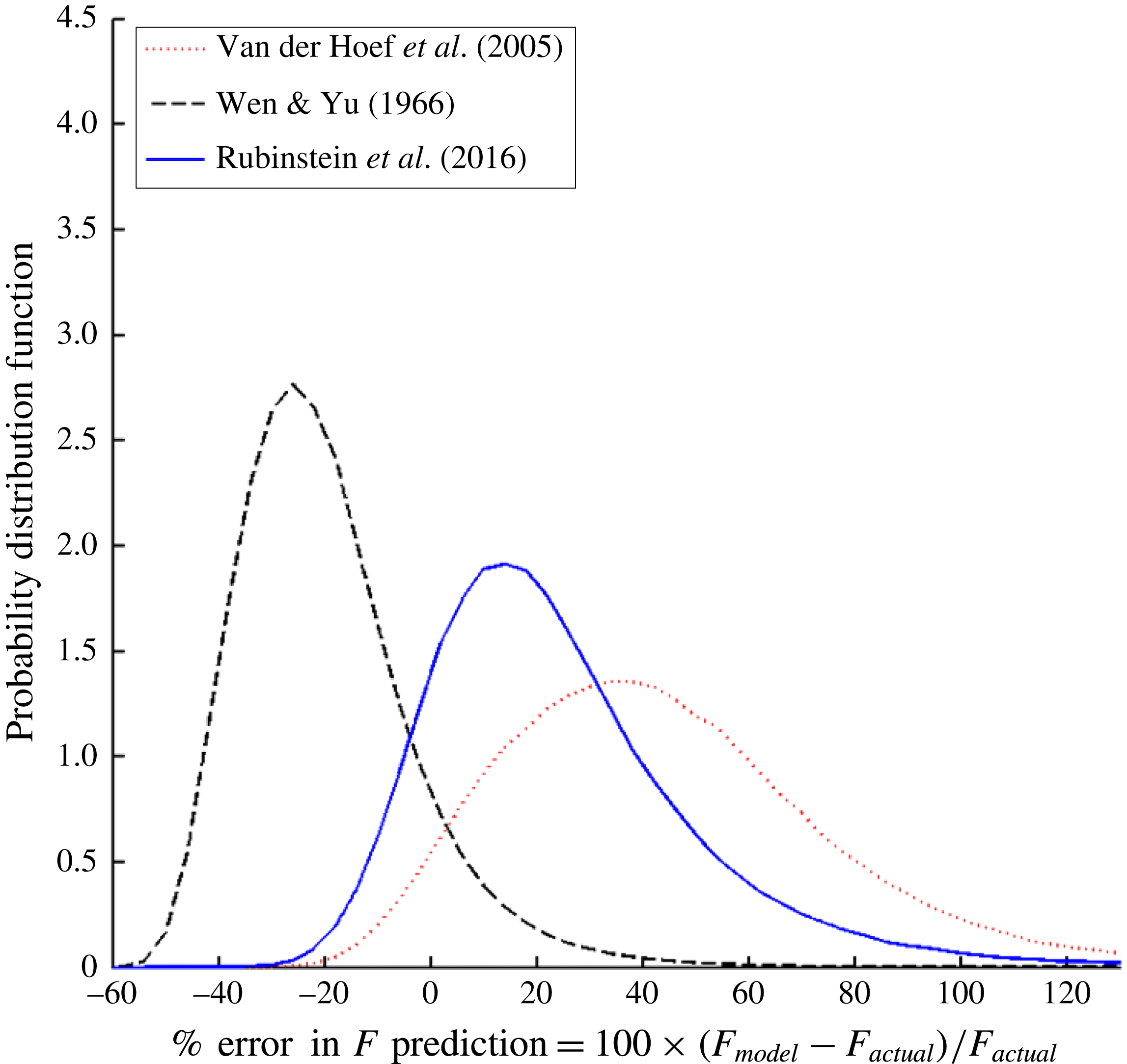
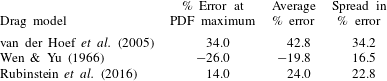
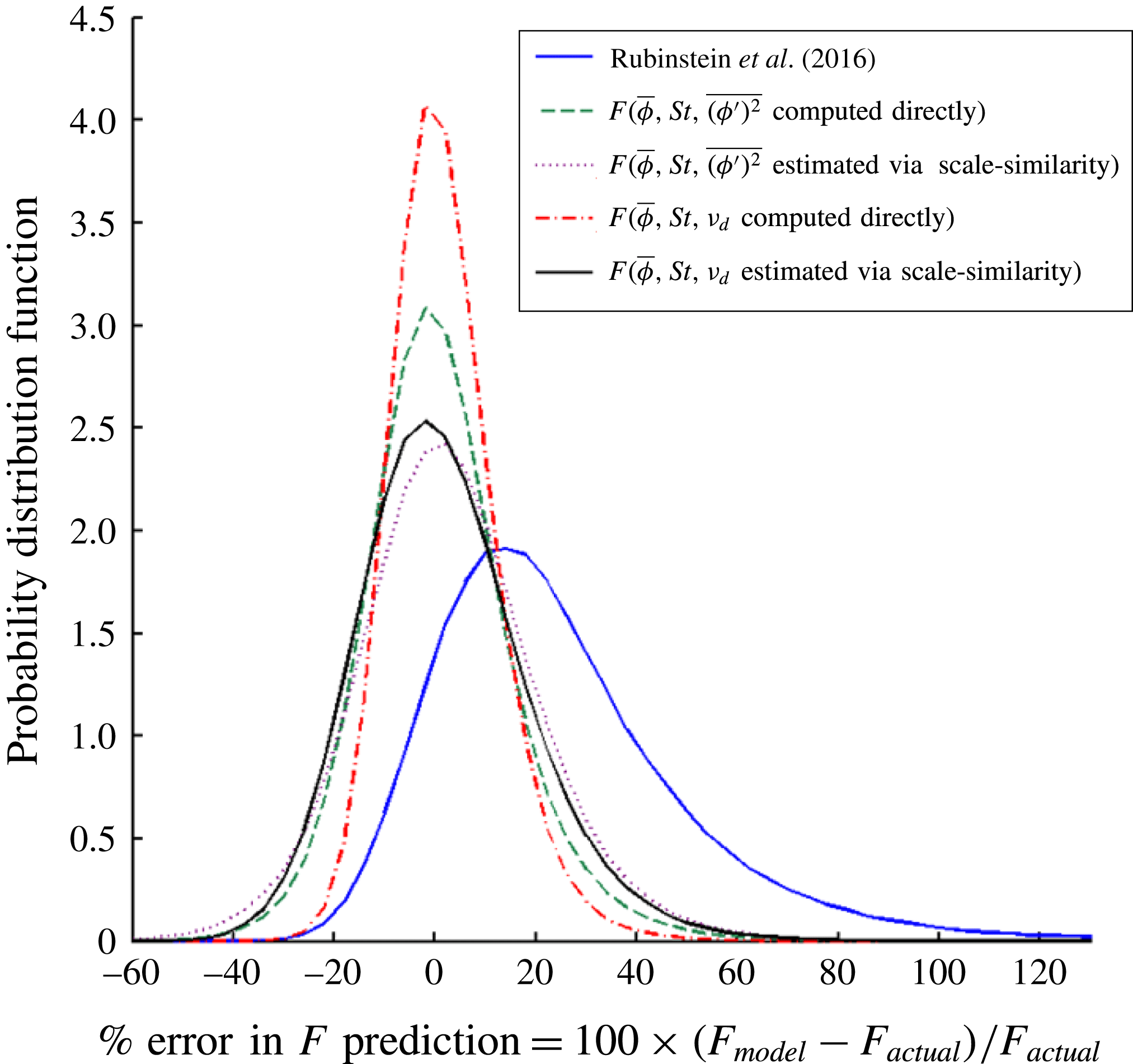
, 0.15, 0.2, 0.25, and 0.3, and these LBM drag values are compared with the drag that is predicted by the following constitutive models: Wen & Yu (Reference Wen and Yu1966), van der Hoef et al. (Reference van der Hoef, Beetstra and Kuipers2005) and Rubinstein et al. (Reference Rubinstein, Derksen and Sundaresan2016). In doing so, the error in the model predictions is computed, and the bias and spread in these predictions models are determined. These results are depicted in figure 4, in which the probability distribution function (PDF) for each model’s percentage error in the drag prediction is plotted.
The probability distribution functions (PDF) are plotted for the percentage error in the drag prediction for three homogeneous drag models: Wen & Yu (Reference Wen and Yu1966), van der Hoef et al. (Reference van der Hoef, Beetstra and Kuipers2005) and Rubinstein et al. (Reference Rubinstein, Derksen and Sundaresan2016). This error analysis is applied to fluidized bed systems with the following set of parameters:
 $\unicode[STIX]{x1D70C}_{p}/\unicode[STIX]{x1D70C}_{f}=4$
, 10, 100, 300, 1500, and 3000 and
 $\langle \unicode[STIX]{x1D719}\rangle =0.1$
, 0.15, 0.2, 0.25, and 0.3. The drag results are computed using
 $\unicode[STIX]{x1D6E5}_{f}/d_{p}=3$
.

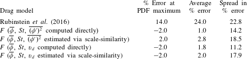
For a given drag prediction error PDF curve, the model bias is computed from both the percentage error at which the PDF is at a maximum and from the average percentage error over the entire distribution. Since the error distributions are slightly skewed towards larger positive errors, the average error is higher than the percentage error at the PDF maximum for all of the drag models. The spread in the percentage error is computed as half the distance between the two percentage error values at which the PDF is at half its maximum. The percentage error at the PDF maximum, average error and spread in the errors are summarized in table 1.
The percentage error at the maximum of the probability distribution functions, the average percentage error, and spread in the distribution of the percentage errors of the homogeneous drag models are presented, when these models are applied, using
 $\unicode[STIX]{x1D6E5}_{f}/d_{p}=3$
, to fluidized bed systems with the following set of parameters:
 $\unicode[STIX]{x1D70C}_{p}/\unicode[STIX]{x1D70C}_{f}=4$
, 10, 100, 300, 1500, and 3000 and
 $\langle \unicode[STIX]{x1D719}\rangle =0.1$
, 0.15, 0.2, 0.25, and 0.3.

As expected, based on the results of figure 4 and table 1, the van der Hoef et al. (Reference van der Hoef, Beetstra and Kuipers2005) model, which is a high-
 $St$
-limit drag relation, is biased towards overpredicting the drag in finite-
 $St$
fluidized beds. Analogously, the Wen & Yu (Reference Wen and Yu1966) model, which is a low-
 $St$
-limit drag relation, is biased towards underpredicting the drag in finite-
 $St$
fluidized beds. The Rubinstein et al. (Reference Rubinstein, Derksen and Sundaresan2016) drag model, which accounts for the effect of
 $St$
, performs better than the two extremes based on the percentage errors at the PDF maximum, and better than the van der Hoef et al. (Reference van der Hoef, Beetstra and Kuipers2005) model based on the average percentage error. Still, on average, there is a significant drag overprediction (
 $+14\,\%$
error at the PDF maximum and
 $+24\,\%$
average error). This significant overprediction is due to the fact that the Rubinstein et al. (Reference Rubinstein, Derksen and Sundaresan2016) model is unable to capture the effects of inhomogeneities, which, as we found in § 3.1, result in a drag reduction. Overall, by analysing the prediction errors of the homogeneous drag models, the need for a new drag model that is able to account for the effects of inhomogeneities is clearly demonstrated.
3.3 Effect of filter size on the behaviour of fluidized beds relative to the high- and low-
 $St$
limits

In our prior study focusing on the effect of
 $St$
(Rubinstein et al.
Reference Rubinstein, Derksen and Sundaresan2016), we found that we could simplify our analysis of the fluid–particle interaction force in a fluidized bed by focusing on the two extreme limits of behaviour: high- and low-
 $St$
-limit beds. In order to connect our findings at these two limits to the behaviour of a particular fluidized bed, we developed the parameter,
 $\unicode[STIX]{x1D6FC}$
, which quantifies the relative magnitude of the drag in a fluidized bed compared to the high- and low-
 $St$
limits:
 $$\begin{eqnarray}\unicode[STIX]{x1D6FC}={\displaystyle \frac{F_{fluidized}-F_{low\,St,\,inhom}}{F_{high\,St,\,inhom}-F_{low\,St,\,inhom}}},\end{eqnarray}$$
where
 $F_{fluidized}$
is the dimensionless drag of the fluidized system. In (3.2),
 $F_{high\,St,\,inhom}$
and
 $F_{low\,St,\,inhom}$
are the drag values computed from the high- and low-
 $St$
-limit bed simulations, respectively, which utilize the inhomogeneous configuration of particles that is taken directly from the fluidized system. In our prior work (Rubinstein et al.
Reference Rubinstein, Derksen and Sundaresan2016), we computed
 $\unicode[STIX]{x1D6FC}$
over the full domain size (
 $\unicode[STIX]{x1D6E5}_{b}=\unicode[STIX]{x1D6E5}_{f}=n_{x}$
). In doing so, we found that the results collapse onto a single curve for
 $\unicode[STIX]{x1D6FC}$
as a function of the modified Stokes number,
 $\tilde{St}$
(defined in (2.5)). The domain-averaged function for
 $\unicode[STIX]{x1D6FC}(\tilde{St})$
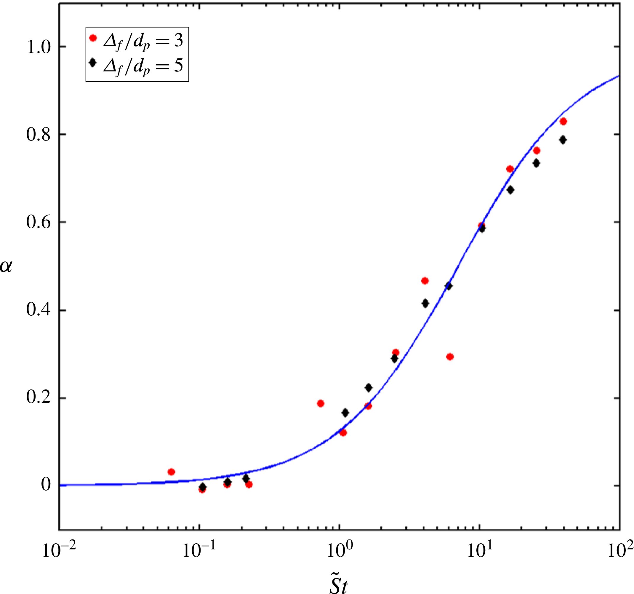
is given in (2.4). In the present study, we extended this analysis to filter sizes smaller than the domain size, as demonstrated in figure 5. In our current analysis,
 $\unicode[STIX]{x1D6E5}_{b}/d_{p}=1$
, and
 $\unicode[STIX]{x1D6FC}$
is computed with
 $\unicode[STIX]{x1D6E5}_{f}/d_{p}=3$
and 5, using fluidized bed simulations with
 $\unicode[STIX]{x1D70C}_{p}/\unicode[STIX]{x1D70C}_{f}=4$
, 10, 100, 300, 1500, and 3000 and
 $\langle \unicode[STIX]{x1D719}\rangle =0.1$
, 0.15, 0.2, 0.25, and 0.3. In terms of filtered quantities, the modified Stokes number,
 $\tilde{St}$
, is defined as:
 $$\begin{eqnarray}\tilde{St}={\displaystyle \frac{\unicode[STIX]{x1D70C}_{p}|\tilde{\boldsymbol{u}}_{slip}|d_{p}}{18\unicode[STIX]{x1D707}_{f}(1-\overline{\unicode[STIX]{x1D719}})}}.\end{eqnarray}$$
 $\tilde{St}$
is the filtered version of the modified Stokes number,
 $St_{mod}$
, defined in (2.5).
The parameter quantifying the behaviour of a fluidized bed relative to the high- and low-
 $St$
limits,
 $\unicode[STIX]{x1D6FC}$
, is plotted as a function of the modified Stokes number,
 $\tilde{St}$
, for different filter sizes:
 $\unicode[STIX]{x1D6E5}_{f}/d_{p}=3$
and 5, with
 $\unicode[STIX]{x1D6E5}_{b}/d_{p}=1$
. These measurements are taken from simulations of fluidized beds with the following set of parameters:
 $\unicode[STIX]{x1D70C}_{p}/\unicode[STIX]{x1D70C}_{f}=4$
, 10, 100, 300, 1500, and 3000 and
 $\langle \unicode[STIX]{x1D719}\rangle =0.1$
, 0.15, 0.2, 0.25, and 0.3. The results for
 $\unicode[STIX]{x1D6FC}$
as a function of
 $\tilde{St}$
fall onto a single curve, which is given by:
 $\unicode[STIX]{x1D6FC}(\tilde{St})=(1/2)(1+(\tilde{St}-7)/(\tilde{St}+7)).$

From figure 5, we see that the results for
 $\unicode[STIX]{x1D6FC}$
as a function of
 $\tilde{St}$
computed using different filter sizes all fall on a single curve, which has the following functional form:
 $$\begin{eqnarray}\unicode[STIX]{x1D6FC}(\tilde{St})={\displaystyle \frac{1}{2}}\left(1+{\displaystyle \frac{\tilde{St}-7}{\tilde{St}+7}}\right).\end{eqnarray}$$
Equation (3.4) is nearly identical to (2.4), which was derived for our prior domain-averaged analysis (Rubinstein et al.
Reference Rubinstein, Derksen and Sundaresan2016), with the small discrepancy in the coefficient that defines the low-to-high-
 $St$
-limit transition point (7 versus 10) due to a limited sensitivity in the results to the choice of
 $\unicode[STIX]{x1D6E5}_{b}$
. The fact that all of the results for
 $\unicode[STIX]{x1D6FC}$
as a function of
 $\tilde{St}$
fall onto a single curve signifies that the relationship between
 $\unicode[STIX]{x1D6FC}$
and
 $\tilde{St}$
persists even as
 $\unicode[STIX]{x1D6E5}_{f}$
varies, which provides us with a powerful relationship between the fluid–particle drag in a fluidized bed and that in the two limiting cases (high- and low-
 $St$
limits). Using this relationship between
 $\unicode[STIX]{x1D6FC}$
and
 $\tilde{St}$
at different length scales, our approach for developing a new drag model that accounts for the effects of inhomogeneities is greatly simplified by our ability to focus on the high- and low-
 $St$
-limit beds, and then interpolate the fluidized bed drag value using the
 $\unicode[STIX]{x1D6FC}(\tilde{St})$
parameter, rather than having to separately study the effect of inhomogeneities on every different type of fluidized bed.
3.4 Quantifying the effect of inhomogeneities
In the low-Re regime, where the effects of fluctuations in the particle velocity on the drag force are negligible, changes in the fluid–particle drag of a fluidized bed relative to the random, homogeneous case are due to the extent of inhomogeneities in the distribution of particles. The key challenge in developing a new drag model, which is able to accurately describe the behaviour of fluidized beds with a wide range of inhomogeneous structures, is therefore to identify how to properly quantify the extent of inhomogeneities. In the current study, three different measures are proposed to quantify the extent of inhomogeneities: the components of the gradient in the particle volume fraction that are perpendicular to the slip velocity,
 $\unicode[STIX]{x1D735}\overline{\unicode[STIX]{x1D719}}_{\bot }$
, the scalar variance of the particle volume fraction,
 $\overline{(\unicode[STIX]{x1D719}^{\prime })^{2}}$
, and the drift flux,
 $\overline{\unicode[STIX]{x1D719}}\tilde{\boldsymbol{v}}_{drift}$
. For the purposes of developing a drag model, the two vector quantities,
 $\unicode[STIX]{x1D735}\overline{\unicode[STIX]{x1D719}}_{\bot }$
and
 $\overline{\unicode[STIX]{x1D719}}\tilde{\boldsymbol{v}}_{drift}$
, are converted into scalars, as discussed in §§ 3.4.1 and 3.4.3, respectively.
As summarized in §§ 1 and 3.1,
 $\unicode[STIX]{x1D735}\overline{\unicode[STIX]{x1D719}}$
has previously been shown by Zhou et al. (Reference Zhou, Xiong, Wang, Wang, Ren and Ge2014) and Li et al. (Reference Li, Wang, Rogers, Zhou and Ge2017) to be a significant measure for determining changes in the drag due to changes in the extents of inhomogeneities, with
 $\unicode[STIX]{x1D735}\overline{\unicode[STIX]{x1D719}}_{\bot }$
, in particular, directly correlated with drag reduction. The two other measures for the extent of inhomogeneities,
 $\overline{(\unicode[STIX]{x1D719}^{\prime })^{2}}$
and
 $\overline{\unicode[STIX]{x1D719}}\tilde{\boldsymbol{v}}_{drift}$
, provide additional insight into the effect of inhomogeneities due to their ability to capture subgrid-scale structures. The scalar variance of the particle volume fraction,
 $\overline{(\unicode[STIX]{x1D719}^{\prime })^{2}}$
, is defined as:
 $$\begin{eqnarray}\overline{(\unicode[STIX]{x1D719}^{\prime })^{2}}=\overline{\unicode[STIX]{x1D719}^{2}}-\overline{\unicode[STIX]{x1D719}}^{2}.\end{eqnarray}$$
This form of
 $\overline{(\unicode[STIX]{x1D719}^{\prime })^{2}}$
was previously employed in the context of turbulent combustion modelling by Jiménez et al. (Reference Jiménez, Ducros, Cuenot and Bédat2001), and later used in the context of multiphase flow modelling by Ozel et al. (Reference Ozel, Fede and Simonin2013). The drift flux,
 $\overline{\unicode[STIX]{x1D719}}\tilde{\boldsymbol{v}}_{drift}$
, measures the correlation between
 $\boldsymbol{u}_{slip}$
and
 $\unicode[STIX]{x1D719}$
, and is defined as:
 $$\begin{eqnarray}\overline{\unicode[STIX]{x1D719}}\tilde{\boldsymbol{v}}_{drift}=\overline{\boldsymbol{u}_{slip}\unicode[STIX]{x1D719}}-\tilde{\boldsymbol{u}}_{slip}\overline{\unicode[STIX]{x1D719}}.\end{eqnarray}$$
This drift flux measure was derived concurrently by Simonin and co-workers (Ozel et al. Reference Ozel, Parmentier, Simonin and Fede2010; Parmentier et al. Reference Parmentier, Simonin and Delsart2012; Ozel et al. Reference Ozel, Fede and Simonin2013) and in the work of Fox (Reference Fox2014). In the next three sections, the effect of each of these three quantities on the drag is further analysed.
In the current study, filter sizes of 3 and 5
 $d_{p}$
are employed in order to investigate the effect of inhomogeneities on the drag. Due to the multiscale hierarchy of the complex structures that develop in a fluidized system, the drag derived in a microscale LBM simulation still cannot be directly applied to an industrial-scale TFM or CFD-DEM simulation, which, due to computational restrictions, must have a grid size on the order of 100
 $d_{p}$
. Instead, the goal of this study is to develop a microscale drag model that can be applied as a constitutive closure to TFM and CFD-DEM simulations at the mesoscale, where the grid size is
 ${\sim}5d_{p}$
. For those needs, the range of filter sizes that are currently studied are most appropriate. In order to properly account for the effects of the mesoscale structures when simulating industrial-scale fluidized beds, the grid size in the TFM and CFD-DEM simulations needs to be significantly coarsened using a filtering technique, in which a filtered drag relation is derived using mesoscale simulations (Igci & Sundaresan Reference Igci and Sundaresan2011; Ozel et al.
Reference Ozel, Fede and Simonin2013).
3.4.1 Gradient in the particle volume fraction
Drawing upon the insights determined by Zhou et al. (Reference Zhou, Xiong, Wang, Wang, Ren and Ge2014) and Li et al. (Reference Li, Wang, Rogers, Zhou and Ge2017), we sought to study the effect of gradients in the particle volume fraction on the fluid–particle drag force. Since, in § 3.1, we found that the dominant effect of inhomogeneities is to produce a reduction in drag, our focus in this study is on
 $\unicode[STIX]{x1D735}\overline{\unicode[STIX]{x1D719}}_{\bot }$
. In particular, we utilized the following non-dimensional, scalar measure:
 $\unicode[STIX]{x1D6E5}_{f}|\unicode[STIX]{x1D735}\overline{\unicode[STIX]{x1D719}}_{\bot }|$
. Since this gradient measure is based solely on the configuration of particles, we are able to, based on the conclusions of § 3.3, study the fluidized bed particle configurations using the high- and low-
 $St$
-limit simulations, and then interpolate these results to the behaviour of fluidized beds using
 $\unicode[STIX]{x1D6FC}(\tilde{St})$
, as defined in (3.4).
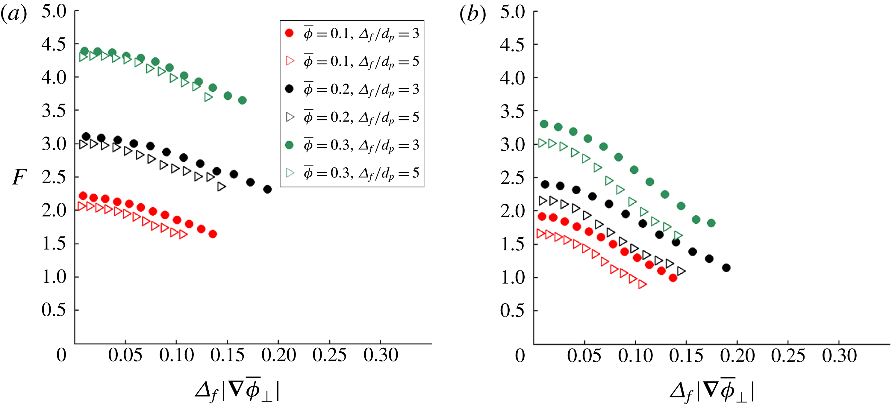
In figure 6, the dimensionless drag force,
 $F$
, is plotted as a function of
 $\unicode[STIX]{x1D6E5}_{f}|\unicode[STIX]{x1D735}\overline{\unicode[STIX]{x1D719}}_{\bot }|$
for the (a) high- and (b) low-
 $St$
limits. These results are compiled from particle configurations taken from fluidized beds with the following set of parameters:
 $\unicode[STIX]{x1D70C}_{p}/\unicode[STIX]{x1D70C}_{f}=4$
, 10, 100, 300, 1500, and 3000 and
 $\langle \unicode[STIX]{x1D719}\rangle =0.1$
, 0.15, 0.2, 0.25, and 0.3. For the analysis shown in figure 6,
 $F$
is computed using a range of filter sizes (
 $\unicode[STIX]{x1D6E5}_{f}/d_{p}=3$
and 5) and bin-averaged with both
 $\overline{\unicode[STIX]{x1D719}}$
(using a bin width of 0.01) and
 $\unicode[STIX]{x1D6E5}_{f}|\unicode[STIX]{x1D735}\overline{\unicode[STIX]{x1D719}}_{\bot }|$
. In order to demonstrate the effect of
 $\unicode[STIX]{x1D6E5}_{f}|\unicode[STIX]{x1D735}\overline{\unicode[STIX]{x1D719}}_{\bot }|$
on
 $F$
, the results are shown for the following
 $\overline{\unicode[STIX]{x1D719}}$
-bins:
 $\overline{\unicode[STIX]{x1D719}}=0.1$
, 0.2, and 0.3. From figure 6(a,b), we observe that, as expected, there is a reduction in drag as
 $\unicode[STIX]{x1D6E5}_{f}|\unicode[STIX]{x1D735}\overline{\unicode[STIX]{x1D719}}_{\bot }|$
increases for both the high- and low-
 $St$
limits. This trend holds even as
 $\overline{\unicode[STIX]{x1D719}}$
and
 $\unicode[STIX]{x1D6E5}_{f}$
are both varied.
The dimensionless drag force,
 $F$
, is plotted as a function of the dimensionless magnitude of the gradient in particle volume fraction that is perpendicular to the slip velocity,
 $\unicode[STIX]{x1D6E5}_{f}|\unicode[STIX]{x1D735}\overline{\unicode[STIX]{x1D719}}_{\bot }|$
, for the (a) high-
 $St$
limit and (b) low-
 $St$
limit. For both of these cases, the results are shown for
 $\overline{\unicode[STIX]{x1D719}}=0.1$
, 0.2, and 0.3 and
 $\unicode[STIX]{x1D6E5}_{f}/d_{p}=3$
and 5. These results are compiled from particle configurations taken from fluidized beds with the following set of parameters:
 $\unicode[STIX]{x1D70C}_{p}/\unicode[STIX]{x1D70C}_{f}=4$
, 10, 100, 300, 1500, and 3000 and
 $\langle \unicode[STIX]{x1D719}\rangle =0.1$
, 0.15, 0.2, 0.25, and 0.3.

In order to develop a new
 $\unicode[STIX]{x1D6E5}_{f}|\unicode[STIX]{x1D735}\overline{\unicode[STIX]{x1D719}}_{\bot }|$
-dependent drag model that can be applied to larger-scale simulations over a range of length scales, it is essential for the trends in the drag force to persist as the filter size is varied. However, from figure 6(a,b), it is clear that the results for
 $F$
as a function of
 $\unicode[STIX]{x1D6E5}_{f}|\unicode[STIX]{x1D735}\overline{\unicode[STIX]{x1D719}}_{\bot }|$
do not lie on a single curve as
 $\unicode[STIX]{x1D6E5}_{f}$
is varied for both the high- and low-
 $St$
limits. This discrepancy in the trends is especially pronounced in the low-
 $St$
-limit case. Instead, it appears that as
 $\unicode[STIX]{x1D6E5}_{f}$
increases, there is a clear reduction in drag for the same value of
 $\overline{\unicode[STIX]{x1D719}}$
and
 $\unicode[STIX]{x1D6E5}_{f}|\unicode[STIX]{x1D735}\overline{\unicode[STIX]{x1D719}}_{\bot }|$
. Choosing the characteristic length scale for the gradient in the volume fraction to be
 $d_{p}$
instead of
 $\unicode[STIX]{x1D6E5}_{f}$
does not result in a better collapse of the results (not shown in figure 6). Since the
 $\unicode[STIX]{x1D6E5}_{f}|\unicode[STIX]{x1D735}\overline{\unicode[STIX]{x1D719}}_{\bot }|$
measure is only capable of detecting inhomogeneities at the scale of the filter size or larger, it appears that at larger filter sizes, the inability of this measure to capture key subgrid structures, which prior larger-scale filtering studies (Igci & Sundaresan Reference Igci and Sundaresan2011; Schneiderbauer & Pirker Reference Schneiderbauer and Pirker2014) have found to have the most significant effect on the drag, prevents it from being a useful method for quantifying the extent of inhomogeneities.
3.4.2 Scalar variance of the particle volume fraction
The scalar variance of the particle volume fraction,
 $\overline{(\unicode[STIX]{x1D719}^{\prime })^{2}}$
, provides a measure for the extent of fluctuations in the volume fraction at the subgrid scale. Using
 $\overline{(\unicode[STIX]{x1D719}^{\prime })^{2}}$
, as defined in (3.5), we sought to model the reduction in drag due to the effects of inhomogeneities. As was the case for the
 $\unicode[STIX]{x1D6E5}_{f}|\unicode[STIX]{x1D735}\overline{\unicode[STIX]{x1D719}}_{\bot }|$
measure in § 3.4.1, since
 $\overline{(\unicode[STIX]{x1D719}^{\prime })^{2}}$
is solely based on the configuration of particles, we are able to study the fluidized bed particle configurations using the high- and low-
 $St$
limit simulations, and then interpolate these results to the behaviour of fluidized beds using
 $\unicode[STIX]{x1D6FC}(\tilde{St})$
(3.4).
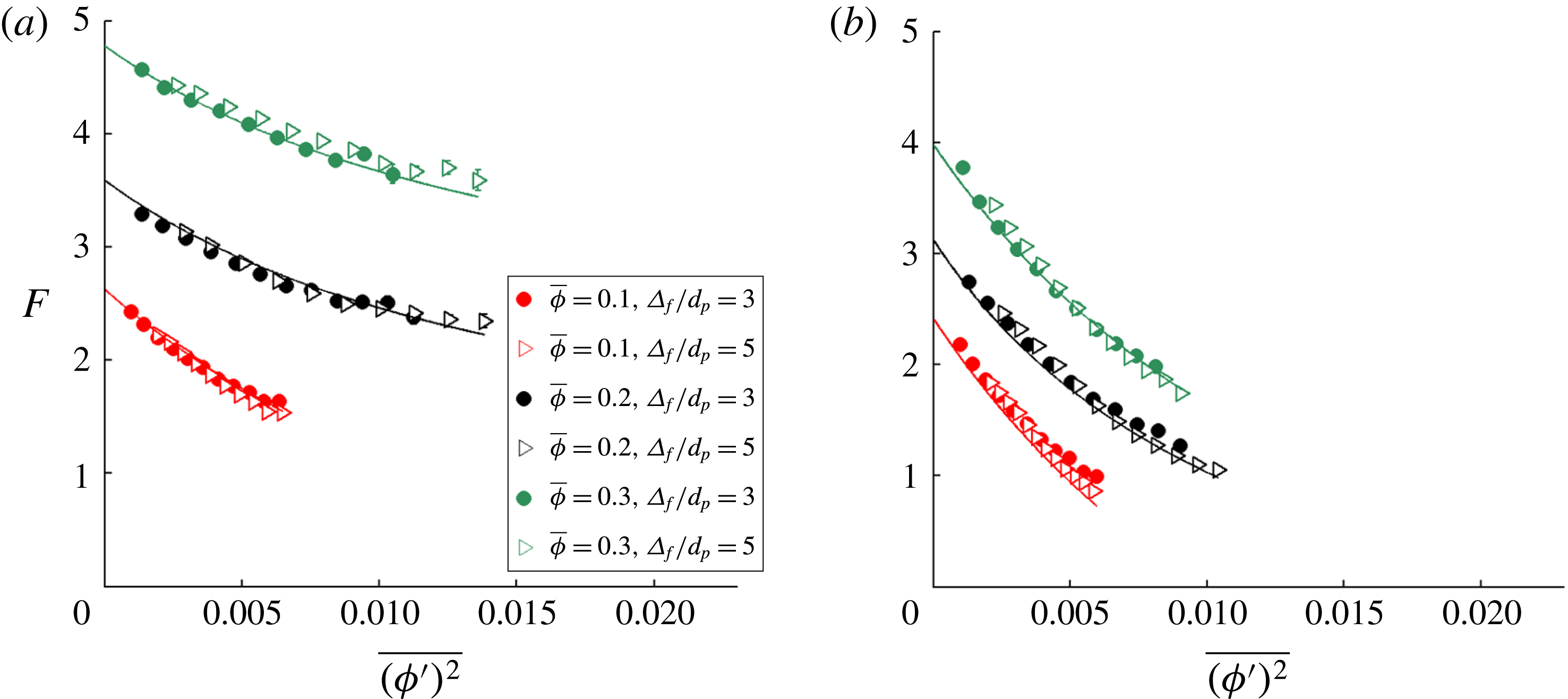
In figure 7, the dimensionless drag force,
 $F$
, is plotted as a function of
 $\overline{(\unicode[STIX]{x1D719}^{\prime })^{2}}$
for the (a) high- and (b) low-
 $St$
limits.
 $F$
is computed using a range of filter sizes (
 $\unicode[STIX]{x1D6E5}_{f}/d_{p}=3$
and 5) and bin-averaged with both
 $\overline{\unicode[STIX]{x1D719}}$
and
 $\overline{(\unicode[STIX]{x1D719}^{\prime })^{2}}$
. These results are compiled from particle configurations taken from fluidized beds with the following set of parameters:
 $\unicode[STIX]{x1D70C}_{p}/\unicode[STIX]{x1D70C}_{f}=4$
, 10, 100, 300, 1500, and 3000 and
 $\langle \unicode[STIX]{x1D719}\rangle =0.1$
, 0.15, 0.2, 0.25, and 0.3. In order to demonstrate the effect of
 $\overline{(\unicode[STIX]{x1D719}^{\prime })^{2}}$
on
 $F$
, the results are shown for the following
 $\overline{\unicode[STIX]{x1D719}}$
-bins:
 $\overline{\unicode[STIX]{x1D719}}=0.1$
, 0.2, and 0.3. From figures 7(a,b), we observe that, over a range of
 $\overline{\unicode[STIX]{x1D719}}$
and
 $\unicode[STIX]{x1D6E5}_{f}$
values, there is a strong reduction in drag as
 $\overline{(\unicode[STIX]{x1D719}^{\prime })^{2}}$
increases for both the high- and low-
 $St$
limits. In fact, in low-
 $St$
-limit systems at
 $\overline{\unicode[STIX]{x1D719}}=0.1$
, there is a
 $54\,\%$
reduction in the
 $\overline{(\unicode[STIX]{x1D719}^{\prime })^{2}}$
-bin-averaged dimensionless drag force,
 $F$
, over the range of observed
 $\overline{(\unicode[STIX]{x1D719}^{\prime })^{2}}$
values, computed using
 $\unicode[STIX]{x1D6E5}_{f}=3d_{p}$
. This strong reduction in
 $F$
is completely undetected by prior drag relations that do not account for the extent of inhomogeneities.
The dimensionless drag force,
 $F$
, is plotted as a function of the scalar variance in particle volume fraction,
 $\overline{(\unicode[STIX]{x1D719}^{\prime })^{2}}$
, for the (a) high-
 $St$
limit and (b) low-
 $St$
limit. For both of these cases, the results are shown for
 $\overline{\unicode[STIX]{x1D719}}=0.1$
, 0.2, and 0.3 and
 $\unicode[STIX]{x1D6E5}_{f}/d_{p}=3$
and 5. These results are compiled from particle configurations taken from fluidized beds with the following set of parameters:
 $\unicode[STIX]{x1D70C}_{p}/\unicode[STIX]{x1D70C}_{f}=4$
, 10, 100, 300, 1500, and 3000 and
 $\langle \unicode[STIX]{x1D719}\rangle =0.1$
, 0.15, 0.2, 0.25, and 0.3. The curves, derived from the new drag model (3.7) and (3.8) that best fits this data, are shown in these figures.

In contrast to the observations made from figure 6 for the
 $\unicode[STIX]{x1D6E5}_{f}|\unicode[STIX]{x1D735}\overline{\unicode[STIX]{x1D719}}_{\bot }|$
measure, in figure 7, we clearly see that, for a particular value of
 $\overline{\unicode[STIX]{x1D719}}$
, the results for
 $F$
as a function of
 $\overline{(\unicode[STIX]{x1D719}^{\prime })^{2}}$
lie on a single curve as
 $\unicode[STIX]{x1D6E5}_{f}$
is varied. Such a result suggests that
 $\overline{(\unicode[STIX]{x1D719}^{\prime })^{2}}$
provides a powerful measure for the extent of inhomogeneities over a range of length scales. Even at larger filter sizes,
 $\overline{(\unicode[STIX]{x1D719}^{\prime })^{2}}$
is still able to capture the effects of key subgrid-scale structures. Having established the utility of the
 $\overline{(\unicode[STIX]{x1D719}^{\prime })^{2}}$
measure, we then sought to model the drag results at both the high- and low-
 $St$
limits. The high-
 $St$
-limit and low-
 $St$
-limit drag models are written as:
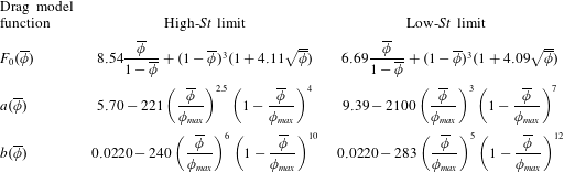
 $$\begin{eqnarray}\displaystyle & \displaystyle F_{high\,St}(\overline{\unicode[STIX]{x1D719}},\,\overline{(\unicode[STIX]{x1D719}^{\prime })^{2}})=F_{0,\,high\,St}(\overline{\unicode[STIX]{x1D719}})-a_{high\,St}(\overline{\unicode[STIX]{x1D719}}){\displaystyle \frac{\overline{(\unicode[STIX]{x1D719}^{\prime })^{2}}/b_{high\,St}(\overline{\unicode[STIX]{x1D719}})}{1+\overline{(\unicode[STIX]{x1D719}^{\prime })^{2}}/b_{high\,St}(\overline{\unicode[STIX]{x1D719}})}}, & \displaystyle\end{eqnarray}$$
 $$\begin{eqnarray}\displaystyle & \displaystyle F_{low\,St}(\overline{\unicode[STIX]{x1D719}},\,\overline{(\unicode[STIX]{x1D719}^{\prime })^{2}})=F_{0,\,low\,St}(\overline{\unicode[STIX]{x1D719}})-a_{low\,St}(\overline{\unicode[STIX]{x1D719}}){\displaystyle \frac{\overline{(\unicode[STIX]{x1D719}^{\prime })^{2}}/b_{low\,St}(\overline{\unicode[STIX]{x1D719}})}{1+\overline{(\unicode[STIX]{x1D719}^{\prime })^{2}}/b_{low\,St}(\overline{\unicode[STIX]{x1D719}})}}. & \displaystyle\end{eqnarray}$$
In (3.7) and (3.8), the model functions
 $F_{0}$
,
 $a$
, and
 $b$
are defined in table 2. The functional form of
 $F_{0}$
in table 2 is inspired by the van der Hoef et al. (Reference van der Hoef, Beetstra and Kuipers2005) drag model in (2.2). The functional form of
 $a$
and
 $b$
in table 2 is empirically derived from this simulation study.
The
 $\overline{(\unicode[STIX]{x1D719}^{\prime })^{2}}$
-dependent drag model functions,
 $F_{0}$
,
 $a$
, and
 $b$
, are presented for both the high- and low-
 $St$
limits, with
 $\unicode[STIX]{x1D719}_{max}=0.64$
.
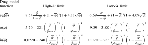
The solid curves drawn in figure 7(a,b) are based on the drag models in (3.7) and (3.8), respectively. The ability of these high- and low-
 $St$
-limit drag relations to accurately fit the drag results over a range of
 $\overline{\unicode[STIX]{x1D719}}$
and
 $\overline{(\unicode[STIX]{x1D719}^{\prime })^{2}}$
demonstrates the success of our model development.
Using the high- and low-
 $St$
-limit drag models, we then interpolate the drag value for a fluidized bed with the following equation:
 $$\begin{eqnarray}F(\overline{\unicode[STIX]{x1D719}},\tilde{St},\overline{(\unicode[STIX]{x1D719}^{\prime })^{2}})=\unicode[STIX]{x1D6FC}(\tilde{St})F_{high\,St}(\overline{\unicode[STIX]{x1D719}},\overline{(\unicode[STIX]{x1D719}^{\prime })^{2}})+(1-\unicode[STIX]{x1D6FC}(\tilde{St}))F_{low\,St}(\overline{\unicode[STIX]{x1D719}},\,\overline{(\unicode[STIX]{x1D719}^{\prime })^{2}}),\end{eqnarray}$$
where
 $\unicode[STIX]{x1D6FC}(\tilde{St})$
is defined in (3.4) and
 $\tilde{St}$
is defined in (3.3). Using (3.7)–(3.9), we are able to define a new
 $\overline{(\unicode[STIX]{x1D719}^{\prime })^{2}}$
-dependent drag model that accounts for the effects of inhomogeneities over a range of length scales. In applying this drag relation as a closure to larger-scale simulations, where the flow is not resolved down to the
 $1d_{p}$
scale, a method for estimating
 $\overline{(\unicode[STIX]{x1D719}^{\prime })^{2}}$
is needed. In order to estimate the value of this quantity, we need to solve an additional transport equation for
 $\overline{(\unicode[STIX]{x1D719}^{\prime })^{2}}$
or employ a scale-similarity approach, as described in § 3.5.1.
3.4.3 Drift flux
As an alternative to defining a drag model in terms of
 $\overline{(\unicode[STIX]{x1D719}^{\prime })^{2}}$
, we can also define a drag model in which the extent of inhomogeneities is captured through the drift flux (Ozel et al.
Reference Ozel, Fede and Simonin2013), as defined in (3.6). This quantity is based not only on the configuration of particles, but also on how the flow structures correlate with particle distributions. A normalized measure for the drift flux is given as:
 $$\begin{eqnarray}v_{d}={\displaystyle \frac{(\overline{\unicode[STIX]{x1D719}}\tilde{\boldsymbol{v}}_{drift})\boldsymbol{\cdot }\tilde{\boldsymbol{u}}_{slip}}{\tilde{\boldsymbol{u}}_{slip}\boldsymbol{\cdot }\tilde{\boldsymbol{u}}_{slip}}}.\end{eqnarray}$$
 $v_{d}$
, which is a scalar quantity, is defined as the normalized component of the drift flux that is in the direction of the slip velocity. Since we found that the magnitude of the drift flux components perpendicular to the slip velocity is negligible
 $({<}1\,\%)$
relative to that of the parallel components, we are able to focus solely on the parallel components for the purposes of drag modelling. Since the drift flux is not solely based on the configuration of particles, it is not useful to derive the drag model based on the drift flux only using high- and low-
 $St$
-limit simulations. Thus, we are unable to employ the same methodology for developing a
 $v_{d}$
-dependent drag model as we did with the
 $\overline{(\unicode[STIX]{x1D719}^{\prime })^{2}}$
-based model in § 3.4.2.
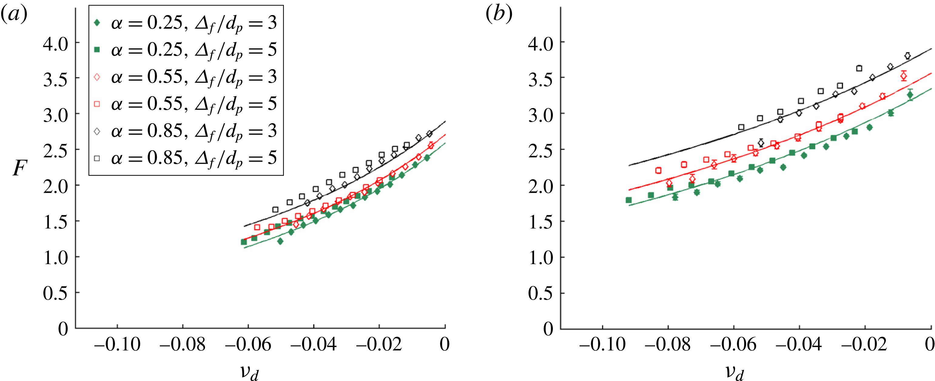
In figure 8,
 $F$
is plotted as a function of
 $v_{d}$
, using the results of fluidized bed simulations with the following set of parameters:
 $\unicode[STIX]{x1D70C}_{p}/\unicode[STIX]{x1D70C}_{f}=4$
, 10, 100, 300, 1500, and 3000 and
 $\langle \unicode[STIX]{x1D719}\rangle =0.1$
, 0.15, 0.2, 0.25, and 0.3.
 $F$
is bin-averaged with
 $\overline{\unicode[STIX]{x1D719}}$
,
 $v_{d}$
, and
 $\unicode[STIX]{x1D6FC}$
for the following filter sizes:
 $\unicode[STIX]{x1D6E5}_{f}/d_{p}=3$
and 5. The value of
 $\unicode[STIX]{x1D6FC}$
, as defined in (3.2), is computed at each filter cell by comparing the drag results in a particular fluidized bed with those in its inhomogeneous high- and low-
 $St$
-limit counterparts. In figure 8(a,b), the results for the
 $\overline{\unicode[STIX]{x1D719}}=0.15$
and
 $\overline{\unicode[STIX]{x1D719}}=0.25$
bins are shown, respectively. In order to fully demonstrate the effect of
 $v_{d}$
on
 $F$
, the results in figure 8 are shown for the following
 $\unicode[STIX]{x1D6FC}$
-bins:
 $\unicode[STIX]{x1D6FC}=0.25$
, 0.55, and 0.85, with
 $\unicode[STIX]{x1D6FC}$
-bin widths of 0.1. From figure 8(a,b), we observe that, over a range of
 $\overline{\unicode[STIX]{x1D719}}$
,
 $\unicode[STIX]{x1D6E5}_{f}$
, and
 $\unicode[STIX]{x1D6FC}$
values, there is a reduction in drag as
 $v_{d}$
becomes more negative. In fact, at
 $\overline{\unicode[STIX]{x1D719}}=0.15$
and
 $\unicode[STIX]{x1D6FC}=0.25$
, there is a
 $49\,\%$
reduction in the
 $v_{d}$
-bin-averaged dimensionless drag force,
 $F$
, over the range of observed drift flux values, computed using
 $\unicode[STIX]{x1D6E5}_{f}=3d_{p}$
. Such a pronounced reduction in
 $F$
cannot be detected by the Rubinstein et al. (Reference Rubinstein, Derksen and Sundaresan2016) model (2.1). It is important to point out that the dimensionless drift flux is primarily negative over the entire fluidized bed system. Since the drift flux is a measure of the correlation between
 $\boldsymbol{u}_{slip}$
and
 $\unicode[STIX]{x1D719}$
, this correlation is typically negative due to the fact that higher values of
 $\unicode[STIX]{x1D719}$
usually result in lower magnitudes of
 $\boldsymbol{u}_{slip}$
.
The dimensionless drag force,
 $F$
, is plotted as a function of the dimensionless drift flux,
 $v_{d}$
, for (a)
 $\overline{\unicode[STIX]{x1D719}}=0.15$
and (b)
 $\overline{\unicode[STIX]{x1D719}}=0.25$
. For both of these cases, the results are shown for
 $\unicode[STIX]{x1D6FC}=0.25$
, 0.55, and 0.85 and
 $\unicode[STIX]{x1D6E5}_{f}/d_{p}=3$
and 5. These results are compiled from fluidized bed simulations with the following set of parameters:
 $\unicode[STIX]{x1D70C}_{p}/\unicode[STIX]{x1D70C}_{f}=4$
, 10, 100, 300, 1500, and 3000 and
 $\langle \unicode[STIX]{x1D719}\rangle =0.1$
, 0.15, 0.2, 0.25, and 0.3. The curves, derived from the new drag model (3.11) that best fits this data, are shown in these figures.

In figure 8, for a particular pair of
 $\overline{\unicode[STIX]{x1D719}}$
and
 $\unicode[STIX]{x1D6FC}$
values, the results for
 $F$
as a function of
 $v_{d}$
fall on a single curve as
 $\unicode[STIX]{x1D6E5}_{f}$
is varied. Such a result suggests that the drift flux provides a powerful measure for the extent of inhomogeneities over a range of length scales. Since
 $v_{d}$
, like
 $\overline{(\unicode[STIX]{x1D719}^{\prime })^{2}}$
, is a subgrid-scale quantity, this measure is still able to capture the effects of key small-scale structures, even at larger filter sizes. Thus, we sought to model the drag as a function of the drift flux.
The drift flux-dependent drag model is defined as follows:
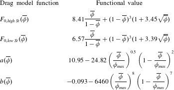
 $$\begin{eqnarray}F(\overline{\unicode[STIX]{x1D719}},\,\tilde{St},\,v_{d})=F_{0}(\overline{\unicode[STIX]{x1D719}},\,\unicode[STIX]{x1D6FC}(\tilde{St}))-a(\overline{\unicode[STIX]{x1D719}}){\displaystyle \frac{v_{d}/b(\overline{\unicode[STIX]{x1D719}})}{1+v_{d}/b(\overline{\unicode[STIX]{x1D719}})}},\end{eqnarray}$$
where
 $F_{0}(\overline{\unicode[STIX]{x1D719}})$
is defined as:
 $$\begin{eqnarray}F_{0}(\overline{\unicode[STIX]{x1D719}},\,\unicode[STIX]{x1D6FC}(\tilde{St}))={\displaystyle \frac{F_{0,high\,St}(\overline{\unicode[STIX]{x1D719}})+F_{0,low\,St}(\overline{\unicode[STIX]{x1D719}})}{2}}+\left({\displaystyle \frac{F_{0,high\,St}(\overline{\unicode[STIX]{x1D719}})-F_{0,low\,St}(\overline{\unicode[STIX]{x1D719}})}{2}}\right){\displaystyle \frac{\text{e}^{10(\unicode[STIX]{x1D6FC}(\tilde{St})-0.6)}-1}{\text{e}^{10(\unicode[STIX]{x1D6FC}(\tilde{St})-0.6)}+1}}.\end{eqnarray}$$
The functional form in (3.12) is based on the functional form for
 $\unicode[STIX]{x1D6FC}(\tilde{St})$
, as given in (3.4), with
 $F_{0}\rightarrow F_{0,high\,St}$
and
 $F_{0}\rightarrow F_{0,low\,St}$
at the high- and low-
 $St$
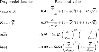
limits, respectively. In (3.11) and (3.12), the model functions
 $F_{0,high\,St}(\overline{\unicode[STIX]{x1D719}})$
,
 $F_{0,low\,St}(\overline{\unicode[STIX]{x1D719}})$
,
 $a(\overline{\unicode[STIX]{x1D719}})$
, and
 $b(\overline{\unicode[STIX]{x1D719}})$
are defined in table 3. The functional form of
 $F_{0,high~St}$
and
 $F_{0,low~St}$
in table 3 is inspired by the van der Hoef et al. (Reference van der Hoef, Beetstra and Kuipers2005) drag model in (2.2). The functional form of
 $a$
and
 $b$
in table 3 is empirically derived from this simulation study.
The drift flux-dependent drag model functions,
 $F_{0,high\,St}$
,
 $F_{0,low\,St}$
,
 $a$
, and
 $b$
, are presented, with
 $\unicode[STIX]{x1D719}_{max}=0.64$
.
The solid curves drawn in figure 8(a,b) are based on the drag model in (3.11). The ability of this drag relation to accurately fit the drag results over a range of
 $\overline{\unicode[STIX]{x1D719}}$
,
 $v_{d}$
, and
 $\unicode[STIX]{x1D6FC}(\tilde{St})$
demonstrates the success of our model development. Using (3.11) and (3.12) and the model functions of table 3, we are able to define a new
 $v_{d}$
-dependent drag model that accounts for the effects of inhomogeneities over a range of length scales. As was the case for the
 $\overline{(\unicode[STIX]{x1D719}^{\prime })^{2}}$
-dependent drag model, in applying this drag relation as a closure to larger-scale simulations, a method for estimating
 $v_{d}$
is needed since the flow is not resolved down to the
 $1d_{p}$
scale. In order to estimate
 $v_{d}$
, we need to solve an additional transport equation for
 $v_{d}$
or employ a scale-similarity approach, as described in § 3.5.2.
3.5 Scale-similar modelling of subgrid-scale quantities
The new drag models that are proposed in § 3.4 quantify the extent of inhomogeneities through one of two subgrid-scale measures:
 $\overline{(\unicode[STIX]{x1D719}^{\prime })^{2}}$
or
 $v_{d}$
. In LBM simulations, the flow is fully resolved at the
 $1d_{p}$
length scale of the base grid cell, and so these quantities can be directly computed using flow information that is available at the subfilter scale. However, when these drag relations are applied as constitutive closures to larger-scale simulations, where the flow is not resolved at the
 $1d_{p}$
length scale and where
 $\unicode[STIX]{x1D6E5}_{f}$
and
 $\unicode[STIX]{x1D6E5}_{b}$
are both taken to be equal to the fluid grid size, the subgrid-scale quantities cannot be directly computed. Thus, a method for estimating these subgrid quantities is needed.
In this study, we employ a scale-similar approach to model the subgrid-scale quantities. This scale-similar approach was first introduced in modelling eddy viscosity in the context of single-phase turbulence by Germano et al. (Reference Germano, Piomelli, Moin and Cabot1991), and was later adapted to drag modelling in large-scale multiphase flow modelling by Parmentier et al. (Reference Parmentier, Simonin and Delsart2012) and Ozel et al. (Reference Ozel, Fede and Simonin2013). Such an approach has not previously been used in the context of developing constitutive models for the fluid–particle drag force using smaller-scale, fully resolved simulations.
In the scale-similar approach, the key assumption made is that the type of inhomogeneous structures that occur at a particular length scale can be predicted based on the type of structures that occur at a second length scale. Thus, using scale-similarity, information available at or above the grid length scale can be used to approximate the subgrid quantities. In order to utilize the scale-similar assumption, a model of the following form needs to be proposed for the subfilter quantities:
 $$\begin{eqnarray}q=\unicode[STIX]{x1D705}\,f(\overline{\unicode[STIX]{x1D719}}/\unicode[STIX]{x1D719}_{max})g(\unicode[STIX]{x1D6E5}_{f}/d_{p}),\end{eqnarray}$$
where
 $q$
is a subgrid-scale measure for the extent of inhomogeneities.
 $f(\overline{\unicode[STIX]{x1D719}}/\unicode[STIX]{x1D719}_{max})$
and
 $g(\unicode[STIX]{x1D6E5}_{f}/d_{p})$
define the functional dependence of the subgrid quantity on the particle concentration and mesh, respectively, and are applicable to fluidized beds with a wide range of system properties. In (3.13),
 $\unicode[STIX]{x1D705}$
is a scalar quantity that adjusts based on the extent of inhomogeneities in a particular system. While
 $\unicode[STIX]{x1D705}$
will vary from system to system, for a particular system, the value of
 $\unicode[STIX]{x1D705}$
will persist over a range of length scales (filter sizes), based on the scale-similarity assumption. The functional form in (3.13) is based on the work of Parmentier et al. (Reference Parmentier, Simonin and Delsart2012) and Ozel et al. (Reference Ozel, Fede and Simonin2013).
In order to proceed with this scale-similar modelling approach, the first step is develop accurate expressions for
 $f$
and
 $g$
. Our development of these models are described in §§ 3.5.1 and 3.5.2 for
 $\overline{(\unicode[STIX]{x1D719}^{\prime })^{2}}$
and
 $v_{d}$
, respectively. Once models for
 $f$
and
 $g$
have been developed, in order to estimate the subgrid quantity in (3.13), we still need a method to approximate the value of
 $\unicode[STIX]{x1D705}$
. In order to take advantage of the scale-similarity assumption,
 $\unicode[STIX]{x1D705}$
is computed through a technique in which the flow structures are analysed using a second, larger filter size, known as the test filter,
 $\unicode[STIX]{x1D6E5}_{f,test}$
. Since the flow is resolved at length scales below
 $\unicode[STIX]{x1D6E5}_{f,test}$
, the use of this test filter approach allows us to compute the extent of subfilter-scale inhomogeneities at the
 $\unicode[STIX]{x1D6E5}_{f,test}$
length scale. Since the value of
 $\unicode[STIX]{x1D705}$
holds at both
 $\unicode[STIX]{x1D6E5}_{f}$
and
 $\unicode[STIX]{x1D6E5}_{f,test}$
, the value of
 $\unicode[STIX]{x1D705}$
can be determined for all of the fluidized bed systems. Having determined
 $f$
,
 $g$
, and
 $\unicode[STIX]{x1D705}$
, the subgrid-scale measure for the extent of inhomogeneities can then be approximated. While some of the mechanics of this test filter approach are presented in § 3.5.1 for the modelling of
 $\overline{(\unicode[STIX]{x1D719}^{\prime })^{2}}$
, further details can be found in the work of Ozel et al. (Reference Ozel, Fede and Simonin2013).
3.5.1 Scalar variance of particle volume fraction
Since
 $\overline{(\unicode[STIX]{x1D719}^{\prime })^{2}}$
is a subgrid-scale measure for the extent of inhomogeneities, we employ a scale-similar approach to estimate this quantity. In order to utilize this approach, the scale-similar form for
 $\overline{(\unicode[STIX]{x1D719}^{\prime })^{2}}$
is defined as:
 $$\begin{eqnarray}\overline{(\unicode[STIX]{x1D719}^{\prime })^{2}}=\unicode[STIX]{x1D705}_{1}f_{1}(\overline{\unicode[STIX]{x1D719}}/\unicode[STIX]{x1D719}_{max})g_{1}(\unicode[STIX]{x1D6E5}_{f}/d_{p}),\end{eqnarray}$$
which is based on the generic scale-similar formalism in (3.13)
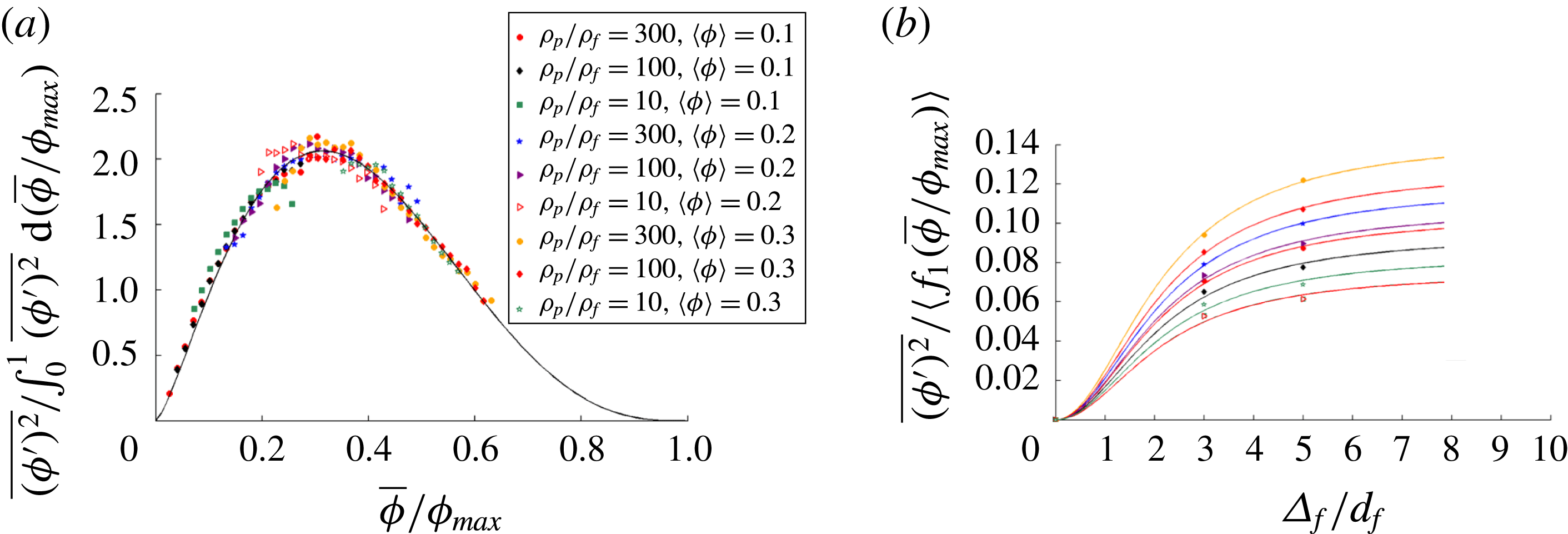
(a) The results for
 $\overline{(\unicode[STIX]{x1D719}^{\prime })^{2}}$
, normalized by
 $\int _{0}^{1}\overline{(\unicode[STIX]{x1D719}^{\prime })^{2}}\,\text{d}(\overline{\unicode[STIX]{x1D719}}/\unicode[STIX]{x1D719}_{max})$
, are shown as a function of
 $\overline{\unicode[STIX]{x1D719}}/\unicode[STIX]{x1D719}_{max}$
. These results are computed using
 $\unicode[STIX]{x1D6E5}_{f}/d_{p}=3$
. The results from the different particle configurations all fall onto a single curve, which we define as:
 $f_{1}(\overline{\unicode[STIX]{x1D719}}/\unicode[STIX]{x1D719}_{max})=(\overline{\unicode[STIX]{x1D719}}/\unicode[STIX]{x1D719}_{max})^{1.37}(1-\overline{\unicode[STIX]{x1D719}}/\unicode[STIX]{x1D719}_{max})^{3.00}.$
(b) The domain-averaged scalar variance results,
 $\langle \overline{(\unicode[STIX]{x1D719}^{\prime })^{2}}\rangle$
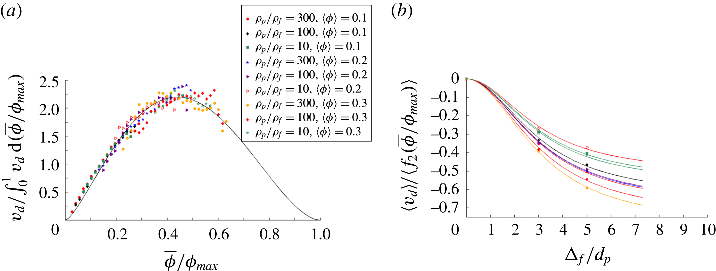
, normalized by
 $\langle f_{1}(\overline{\unicode[STIX]{x1D719}}/\unicode[STIX]{x1D719}_{max})\rangle$
, are shown as a function of
 $\unicode[STIX]{x1D6E5}_{f}/d_{p}$
. The results from the different particle configurations are all modelled using a single function,
 $\langle \unicode[STIX]{x1D705}_{1}\rangle g_{1}(\unicode[STIX]{x1D6E5}_{f}/d_{p})=\langle \unicode[STIX]{x1D705}_{1}\rangle ((\unicode[STIX]{x1D6E5}_{f}/d_{p})^{2}/(4.58+(\unicode[STIX]{x1D6E5}_{f}/d_{p})^{2}))$
, which provides the functional form for the different fitting curves. The results for both of these figures are compiled from particle configurations taken from fluidized beds with the following set of parameters:
 $\unicode[STIX]{x1D70C}_{p}/\unicode[STIX]{x1D70C}_{f}=10$
, 100, and 300 and
 $\langle \unicode[STIX]{x1D719}\rangle =0.1$
, 0.2, and 0.3.

In order to determine a model for
 $f_{1}$
, the dependence of
 $\overline{(\unicode[STIX]{x1D719}^{\prime })^{2}}$
on the concentration of particles, the value of
 $\overline{(\unicode[STIX]{x1D719}^{\prime })^{2}}$
is evaluated for fluidized bed configurations with a wide range of parameters. This analysis is shown in figure 9(a), where
 $f_{1}$
is determined as:
 $$\begin{eqnarray}f_{1}(\overline{\unicode[STIX]{x1D719}}/\unicode[STIX]{x1D719}_{max})={\displaystyle \frac{\overline{(\unicode[STIX]{x1D719}^{\prime })^{2}}}{\displaystyle \displaystyle \int _{0}^{1}\overline{(\unicode[STIX]{x1D719}^{\prime })^{2}}\text{d}(\overline{\unicode[STIX]{x1D719}}/\unicode[STIX]{x1D719}_{max})}}.\end{eqnarray}$$
In order to compute the integral in the denominator of (3.15), a curve is drawn through the results of
 $\overline{(\unicode[STIX]{x1D719}^{\prime })^{2}}$
as a function of
 $\overline{\unicode[STIX]{x1D719}}/\unicode[STIX]{x1D719}_{max}$
from
 $\overline{\unicode[STIX]{x1D719}}/\unicode[STIX]{x1D719}_{max}=0$
to
 $\overline{\unicode[STIX]{x1D719}}/\unicode[STIX]{x1D719}_{max}=1$
.
 $\overline{(\unicode[STIX]{x1D719}^{\prime })^{2}}$
is forced to
 $0$
at these two limits, since there is no variance in the volume fraction when no particles are present and when the particles are at a maximum packing fraction. Using a filter size of
 $\unicode[STIX]{x1D6E5}_{f}/d_{p}=3$
, the results for
 $\overline{(\unicode[STIX]{x1D719}^{\prime })^{2}}/\int _{0}^{1}\overline{(\unicode[STIX]{x1D719}^{\prime })^{2}}\,\text{d}(\overline{\unicode[STIX]{x1D719}}/\unicode[STIX]{x1D719}_{max})$
are then computed as a function of
 $\overline{\unicode[STIX]{x1D719}}/\unicode[STIX]{x1D719}_{max}$
. These results are compiled from particle configurations taken from fluidized beds with the following set of parameters:
 $\unicode[STIX]{x1D70C}_{p}/\unicode[STIX]{x1D70C}_{f}=10$
, 100, and 300 and
 $\langle \unicode[STIX]{x1D719}\rangle =0.1$
, 0.2, and 0.3. From figure 9(a), it is clear that the results from these different configurations all fall onto a single curve, with the following functional form:
 $$\begin{eqnarray}f_{1}(\overline{\unicode[STIX]{x1D719}}/\unicode[STIX]{x1D719}_{max})=(\overline{\unicode[STIX]{x1D719}}/\unicode[STIX]{x1D719}_{max})^{n_{1}}(1-\overline{\unicode[STIX]{x1D719}}/\unicode[STIX]{x1D719}_{max})^{m_{1}},\end{eqnarray}$$
where
 $n_{1}=1.37$
,
 $m_{1}=3.00$
, and
 $\unicode[STIX]{x1D719}_{max}=0.64$
. The function
 $f_{1}(\overline{\unicode[STIX]{x1D719}}/\unicode[STIX]{x1D719}_{max})$
, defined in (3.16) and derived using
 $\unicode[STIX]{x1D6E5}_{f}/d_{p}=3$
, is valid over a range of length scales, as it has also been shown to hold at
 $\unicode[STIX]{x1D6E5}_{f}/d_{p}=5$
to within 4 %. In addition, while figure 9(a) provides only a sampling of the fluidized beds that were simulated in the current study, the universal shape of (3.16) holds over the full range of
 $\unicode[STIX]{x1D70C}_{p}/\unicode[STIX]{x1D70C}_{f}~(4{-}3000)$
and
 $\langle \unicode[STIX]{x1D719}\rangle$
 $(0.1{-}0.3)$
that were investigated. Furthermore, while the high computational demands associated with properly resolving the flow between particles at very high particle volume fractions prevent us from sampling
 $\overline{\unicode[STIX]{x1D719}}$
between 0.4 and
 $\unicode[STIX]{x1D719}_{max}$
in the current work, the fact that the universal shape holds over the entire sampled
 $\overline{\unicode[STIX]{x1D719}}$
and that prior multiphase flow studies employing a scale-similarity technique (Ozel et al.
Reference Ozel, Fede and Simonin2013) have found a similar concentration dependence suggest that (3.16) should hold over the full range of
 $\overline{\unicode[STIX]{x1D719}}$
.
Next, in order to determine a model for
 $g_{1}$
, which defines the mesh dependence of
 $\overline{(\unicode[STIX]{x1D719}^{\prime })^{2}}$
, the properties of
 $\overline{(\unicode[STIX]{x1D719}^{\prime })^{2}}$
are studied over a range of filter sizes. This analysis is shown in figure 9(b), where
 $g_{1}$
is determined as:
 $$\begin{eqnarray}g_{1}(\unicode[STIX]{x1D6E5}_{f}/d_{p})={\displaystyle \frac{\left\langle \overline{(\unicode[STIX]{x1D719}^{\prime })^{2}}\right\rangle }{\langle \unicode[STIX]{x1D705}_{1}f_{1}(\overline{\unicode[STIX]{x1D719}}/\unicode[STIX]{x1D719}_{max})\rangle }},\end{eqnarray}$$
with
 $f_{1}$
defined by (3.16). Performing the domain-averaging operation in (3.17) allows us to determine how, on average,
 $\overline{(\unicode[STIX]{x1D719}^{\prime })^{2}}$
changes with filter size. In figure 9(b), the results for
 $\langle \overline{(\unicode[STIX]{x1D719}^{\prime })^{2}}\rangle /\langle f_{1}(\overline{\unicode[STIX]{x1D719}}/\unicode[STIX]{x1D719}_{max})\rangle$
are shown as a function of
 $\unicode[STIX]{x1D6E5}_{f}/d_{p}$
. The results for each different configuration have the same dependence on
 $\unicode[STIX]{x1D6E5}_{f}/d_{p}$
and
 $g_{1}(\unicode[STIX]{x1D6E5}_{f}/d_{p})$
, and simply vary by the multiplicative constant,
 $\langle \unicode[STIX]{x1D705}_{1}\rangle$
, which defines the extent of inhomogeneities for a particular system, averaged over the domain. This functional dependence on
 $\unicode[STIX]{x1D6E5}_{f}/d_{p}$
is found to be:
 $$\begin{eqnarray}g_{1}(\unicode[STIX]{x1D6E5}_{f}/d_{p})={\displaystyle \frac{(\unicode[STIX]{x1D6E5}_{f}/d_{p})^{2}}{k_{1}+(\unicode[STIX]{x1D6E5}_{f}/d_{p})^{2}}},\end{eqnarray}$$
where
 $k_{1}=4.58$
. While larger computational domains are necessary in order to fully probe the validity of the quadratic mesh dependence in the smaller filter size regime, the form of (3.18) is confirmed in the current study through its ability to effectively pass through all of the data points in figure 9(b) and by the fact that this equation is consistent with the Taylor series expansion of the drift velocity that is performed by Ozel et al. (Reference Ozel, Fede and Simonin2013). The value for
 $k_{1}$
is determined based on a best fit of the simulation data points in figure 9(b). The curves, based on
 $\langle \unicode[STIX]{x1D705}_{1}\rangle g_{1}(\unicode[STIX]{x1D6E5}_{f}/d_{p})$
, are shown, in figure 9(b), to fit the results over a range of system parameters.
 $\unicode[STIX]{x1D705}_{1}$
is found to be larger for particle configurations taken from fluidized beds with larger values of
 $\unicode[STIX]{x1D70C}_{p}/\unicode[STIX]{x1D70C}_{f}$
, due to the fact that these configurations have a larger extent of inhomogeneities. As an example of this trend, for systems with
 $\langle \unicode[STIX]{x1D719}\rangle =0.3$
, the domain-averaged value of
 $\unicode[STIX]{x1D705}_{1}$
is
 $0.084$
and
 $0.143$
for the
 $\unicode[STIX]{x1D70C}_{p}/\unicode[STIX]{x1D70C}_{f}=10$
and
 $\unicode[STIX]{x1D70C}_{p}/\unicode[STIX]{x1D70C}_{f}=300$
configurations, respectively.
Having developed the scale-similar models for
 $f_{1}(\overline{\unicode[STIX]{x1D719}}/\unicode[STIX]{x1D719}_{max})$
and
 $g_{1}(\unicode[STIX]{x1D6E5}_{f}/d_{p})$
,
 $\overline{(\unicode[STIX]{x1D719}^{\prime })^{2}}$
can then be estimated by utilizing the test filter approach, as discussed in § 3.5. Quantities that are filtered using the test filter,
 $\unicode[STIX]{x1D6E5}_{f,test}$
, are denoted with a hat. The scalar variance of the filtered solid volume fraction,
 $\widehat{\overline{(\unicode[STIX]{x1D719}^{\prime })_{\ast }^{2}}}$
, at the test scale is defined as:
 $$\begin{eqnarray}\widehat{\overline{(\unicode[STIX]{x1D719}^{\prime })_{\ast }^{2}}}=\widehat{\overline{\unicode[STIX]{x1D719}^{2}}}-\widehat{\overline{\unicode[STIX]{x1D719}}}^{2}=\unicode[STIX]{x1D705}_{1}f_{1}(\widehat{\overline{\unicode[STIX]{x1D719}}}/\unicode[STIX]{x1D719}_{max})g_{1}(\unicode[STIX]{x1D6E5}_{f,test}/d_{p}),\end{eqnarray}$$
while the test-filtered scalar variance,
 $\widehat{\overline{(\unicode[STIX]{x1D719}^{\prime })^{2}}}$
, is defined as:

From (3.19) and (3.20), we are able to solve for
 $\unicode[STIX]{x1D705}_{1}$
as:

Using this test filter approach, the value of
 $\unicode[STIX]{x1D705}_{1}$
can be estimated throughout the fluidized bed system.
The subgrid-scale measure for the extent of inhomogeneities,
 $\overline{(\unicode[STIX]{x1D719}^{\prime })^{2}}$
, can be approximated through scale-similar modelling using (3.14), (3.16), (3.18), and (3.21). In doing so, this quantity can be estimated in simulations where the flow is not fully resolved.
In (3.18), the parameter
 $k_{1}$
defines how quickly the mesh dependence of
 $\overline{(\unicode[STIX]{x1D719}^{\prime })^{2}}$
is saturated at higher filter sizes, with smaller values of
 $k_{1}$
correlating with this saturation occurring at lower values of
 $\unicode[STIX]{x1D6E5}_{f}$
. The current analysis has been performed using a domain size of
 $n_{x}=12d_{p}$
. In order to determine how this saturation parameter,
 $k_{1}$
, varies with domain size, we have also performed this analysis at other domain sizes (
 $n_{x}=9d_{p}$
and
 $24d_{p}$
). From this analysis, it appears that as the domain size increases, the mesh dependence of
 $\overline{(\unicode[STIX]{x1D719}^{\prime })^{2}}$
becomes saturated at higher filter sizes, and so
 $k_{1}$
increases roughly as the square root of the domain size. Thus, as we look to apply this new drag constitutive relation to large-scale fluidized bed simulations, we can extrapolate this trend in order to conclude that
 $k_{1}\gg (\unicode[STIX]{x1D6E5}_{f}/d_{p})^{2}$
for large-scale systems. Using this relationship, the scale-similar form for
 $\overline{(\unicode[STIX]{x1D719}^{\prime })^{2}}$
can be written in its modified form as:
 $$\begin{eqnarray}\overline{(\unicode[STIX]{x1D719}^{\prime })^{2}}=\unicode[STIX]{x1D705}_{1}^{\prime }f_{1}(\overline{\unicode[STIX]{x1D719}}/\unicode[STIX]{x1D719}_{max})g_{1}^{\prime }(\unicode[STIX]{x1D6E5}_{f}/d_{p}),\end{eqnarray}$$
where
 $\unicode[STIX]{x1D705}_{1}^{\prime }=\unicode[STIX]{x1D705}_{1}/k_{1}$
and
 $g_{1}^{\prime }(\unicode[STIX]{x1D6E5}_{f}/d_{p})=(\unicode[STIX]{x1D6E5}_{f}/d_{p})^{2}$
.
3.5.2 Drift flux
Since the drift flux is a subgrid-scale measure for the extent of inhomogeneities, we employ, as we did for
 $\overline{(\unicode[STIX]{x1D719}^{\prime })^{2}}$
in § 3.5.1, a scale-similar method to estimate this quantity. A scale-similar form for the dimensionless drift flux is given by:
 $$\begin{eqnarray}v_{d}=\unicode[STIX]{x1D705}_{2}f_{2}(\overline{\unicode[STIX]{x1D719}}/\unicode[STIX]{x1D719}_{max})g_{2}(\unicode[STIX]{x1D6E5}_{f}/d_{p}).\end{eqnarray}$$
(a) The results for
 $v_{d}$
, normalized by
 $\int _{0}^{1}v_{d}\,\text{d}(\overline{\unicode[STIX]{x1D719}}/\unicode[STIX]{x1D719}_{max})$
, are shown as a function of
 $\overline{\unicode[STIX]{x1D719}}/\unicode[STIX]{x1D719}_{max}$
. These results are computed using
 $\unicode[STIX]{x1D6E5}_{f}/d_{p}=3$
. The results from the different particle configurations all fall onto a single curve, which we define as:
 $f_{2}(\overline{\unicode[STIX]{x1D719}}/\unicode[STIX]{x1D719}_{max})=(\overline{\unicode[STIX]{x1D719}}/\unicode[STIX]{x1D719}_{max})^{1.44}(1-\overline{\unicode[STIX]{x1D719}}/\unicode[STIX]{x1D719}_{max})^{1.84}.$
(b) The domain-averaged drift flux results,
 $\langle v_{d}\rangle$
, normalized by
 $\langle f_{2}(\overline{\unicode[STIX]{x1D719}}/\unicode[STIX]{x1D719}_{max})\rangle$
, are shown as a function of
 $\unicode[STIX]{x1D6E5}_{f}/d_{p}$
. The results from the different particle configurations are all modelled using a single function,
 $\langle \unicode[STIX]{x1D705}_{2}\rangle g_{2}(\unicode[STIX]{x1D6E5}_{f}/d_{p})=\langle \unicode[STIX]{x1D705}_{2}\rangle ((\unicode[STIX]{x1D6E5}_{f}/d_{p})^{2}/(9.20+(\unicode[STIX]{x1D6E5}_{f}/d_{p})^{2})),$
which provides the functional form for the different fitting curves. The results for both of these figures are compiled from fluidized bed simulations with the following set of parameters:
 $\unicode[STIX]{x1D70C}_{p}/\unicode[STIX]{x1D70C}_{f}=10$
, 100, and 300 and
 $\langle \unicode[STIX]{x1D719}\rangle =0.1$
, 0.2, and 0.3.

In order to determine a model for
 $f_{2}$
, the dependence of
 $v_{d}$
on the concentration of particles, this function, as shown in figure 10(a), is computed as:
 $$\begin{eqnarray}f_{2}(\overline{\unicode[STIX]{x1D719}}/\unicode[STIX]{x1D719}_{max})={\displaystyle \frac{v_{d}}{\displaystyle \int _{0}^{1}v_{d}\,\text{d}(\overline{\unicode[STIX]{x1D719}}/\unicode[STIX]{x1D719}_{max})}}.\end{eqnarray}$$
Like
 $\overline{(\unicode[STIX]{x1D719}^{\prime })^{2}}$
,
 $v_{d}$
is taken to be
 $0$
at the two
 $\overline{\unicode[STIX]{x1D719}}/\unicode[STIX]{x1D719}_{max}$
limits. Using a filter size of
 $\unicode[STIX]{x1D6E5}_{f}/d_{p}=3$
, the results for
 $v_{d}/\!\int _{0}^{1}v_{d}d(\overline{\unicode[STIX]{x1D719}}/\unicode[STIX]{x1D719}_{max})$
are then computed as a function of
 $\overline{\unicode[STIX]{x1D719}}/\unicode[STIX]{x1D719}_{max}$
. The results in figure 10(a) are compiled from fluidized bed simulations with the following set of parameters:
 $\unicode[STIX]{x1D70C}_{p}/\unicode[STIX]{x1D70C}_{f}=10$
, 100, and 300 and
 $\langle \unicode[STIX]{x1D719}\rangle =0.1$
, 0.2, and 0.3. From figure 10(a), it is clear that the results from these different configurations all fall onto a single curve, with the following functional form:
 $$\begin{eqnarray}f_{2}(\overline{\unicode[STIX]{x1D719}}/\unicode[STIX]{x1D719}_{max})=(\overline{\unicode[STIX]{x1D719}}/\unicode[STIX]{x1D719}_{max})^{n_{2}}(1-\overline{\unicode[STIX]{x1D719}}/\unicode[STIX]{x1D719}_{max})^{m_{2}},\end{eqnarray}$$
where
 $n_{2}=1.44$
,
 $m_{2}=1.84$
, and
 $\unicode[STIX]{x1D719}_{max}=0.64$
.
 $f_{2}(\overline{\unicode[STIX]{x1D719}}/\unicode[STIX]{x1D719}_{max})$
is valid over a range of length scales, as it has also been shown to hold at
 $\unicode[STIX]{x1D6E5}_{f}/d_{p}=5$
to within 5 %. In addition, while figure 10(a) provides only a sampling of the fluidized beds that were simulated in the current study, the universal shape of (3.25) holds over the full range of
 $\unicode[STIX]{x1D70C}_{p}/\unicode[STIX]{x1D70C}_{f}$
and
 $\langle \unicode[STIX]{x1D719}\rangle$
that were investigated. Furthermore, given the fact that the universal shape holds over the entire sampled
 $\overline{\unicode[STIX]{x1D719}}~(0{-}0.4)$
and that prior multiphase flow studies employing a scale-similarity technique (Ozel et al.
Reference Ozel, Fede and Simonin2013) have found a similar concentration dependence, the universal shape of (3.25) should hold over the full range of
 $\overline{\unicode[STIX]{x1D719}}$
.
Comparing the results of figure 10(a) with those of figure 9(a), the collapse of the
 $v_{d}$
data points onto a single universal curve is found to be not as strong as that of
 $\overline{(\unicode[STIX]{x1D719}^{\prime })^{2}}$
, especially near the peak of the curve. Since
 $v_{d}$
involves both
 $\overline{\unicode[STIX]{x1D719}}$
and
 $\tilde{\boldsymbol{u}}_{slip}$
, there is a possibility that attaining a universal shape for
 $v_{d}$
as a function of
 $\overline{\unicode[STIX]{x1D719}}$
is more difficult as compared to
 $\overline{(\unicode[STIX]{x1D719}^{\prime })^{2}}$
, which only involves
 $\overline{\unicode[STIX]{x1D719}}$
. Near the peak of the curve in figure 10(a), the overall effects of inhomogeneities are at their most extreme, so any additional effects of inhomogeneities in
 $\tilde{\boldsymbol{u}}_{slip}$
would further complicate the attempts to obtain a collapse of the
 $v_{d}$
data points onto a single curve. Still, based on the fact that the data points in figure 10(a) generally fall onto the universal curve, the scale-similar approach is still found to be appropriate for modelling
 $v_{d}$
.
Next, in order to determine a model for
 $g_{2}$
, the mesh dependence of
 $v_{d}$
, this function, as shown in figure 10(b), is computed as:
 $$\begin{eqnarray}g_{2}(\unicode[STIX]{x1D6E5}_{f}/d_{p})={\displaystyle \frac{\langle v_{d}\rangle }{\langle \unicode[STIX]{x1D705}_{2}f_{2}(\overline{\unicode[STIX]{x1D719}}/\unicode[STIX]{x1D719}_{max})\rangle }},\end{eqnarray}$$
with
 $f_{2}$
defined by (3.25). In figure 10(b), the results for
 $\langle v_{d}\rangle /\langle f_{2}(\overline{\unicode[STIX]{x1D719}}/\unicode[STIX]{x1D719}_{max})\rangle$
are shown as a function of
 $\unicode[STIX]{x1D6E5}_{f}/d_{p}$
. The results for each different configuration have the same dependence on
 $\unicode[STIX]{x1D6E5}_{f}/d_{p}$
, and simply vary by the multiplicative constant,
 $\langle \unicode[STIX]{x1D705}_{2}\rangle$
. For all of these cases,
 $\langle \unicode[STIX]{x1D705}_{2}\rangle <0$
because
 $v_{d}$
is typically negative over the entire fluidized bed, as explained in § 3.4.3. The functional dependence of
 $v_{d}$
on
 $\unicode[STIX]{x1D6E5}_{f}/d_{p}$
is found to be:
 $$\begin{eqnarray}g_{2}(\unicode[STIX]{x1D6E5}_{f}/d_{p})={\displaystyle \frac{(\unicode[STIX]{x1D6E5}_{f}/d_{p})^{2}}{k_{2}+(\unicode[STIX]{x1D6E5}_{f}/d_{p})^{2}}},\end{eqnarray}$$
where
 $k_{2}=9.20$
. While larger computational domains are necessary in order to fully probe the validity of the quadratic mesh dependence in the smaller filter size regime, the form of (3.27) is confirmed in the current study through its ability to effectively pass through all of the data points in figure 10(b) and by the fact that this equation is consistent with the Taylor series expansion of the drift velocity that is performed by Ozel et al. (Reference Ozel, Fede and Simonin2013). The curves, based on
 $\langle \unicode[STIX]{x1D705}_{2}\rangle g_{2}(\unicode[STIX]{x1D6E5}_{f}/d_{p})$
, are shown, in figure 10(b), to fit the results over a range of system parameters. As was true for
 $\unicode[STIX]{x1D705}_{1}$
in § 3.5.1,
 $\unicode[STIX]{x1D705}_{2}$
is found to be larger for particle configurations taken from fluidized beds with larger values of
 $\unicode[STIX]{x1D70C}_{p}/\unicode[STIX]{x1D70C}_{f}$
.
Using a test filter approach similar to the one described in (3.21) for the
 $\overline{(\unicode[STIX]{x1D719}^{\prime })^{2}}$
measure,
 $\unicode[STIX]{x1D705}_{2}$
can be estimated throughout the fluidized bed system as:

Thus, the dimensionless drift flux can be approximated through scale-similar modelling using (3.23), (3.25), (3.27), and (3.28). In doing so,
 $v_{d}$
can be estimated in simulations where the flow is not fully resolved.
Analogous to the domain-size dependence of
 $k_{1}$
, which is discussed in § 3.5.1,
 $k_{2}$
is found to increase with the domain size. Thus, the modified scale-similar model for the drift flux that is applicable to larger-scale simulations is given by:
 $$\begin{eqnarray}v_{d}=\unicode[STIX]{x1D705}_{2}^{\prime }f_{2}(\overline{\unicode[STIX]{x1D719}}/\unicode[STIX]{x1D719}_{max})g_{2}^{\prime }(\unicode[STIX]{x1D6E5}_{f}/d_{p}),\end{eqnarray}$$
where
 $\unicode[STIX]{x1D705}_{2}^{\prime }=\unicode[STIX]{x1D705}_{2}/k_{2}$
and
 $g_{2}^{\prime }(\unicode[STIX]{x1D6E5}_{f}/d_{p})=(\unicode[STIX]{x1D6E5}_{f}/d_{p})^{2}$
.
Further details for implementing the inhomogeneity-dependent constitutive closures for the fluid–particle drag force can be found in the supplementary material available at https://doi.org/10.1017/jfm.2017.705.
3.6 Error analysis of new drag models
In order to conduct an analysis of these newly developed drag models, the filtered
 $(\unicode[STIX]{x1D6E5}_{f}/d_{p}=3)$
, dimensionless drag,
 $F$
, is computed via fully resolved simulations in fluidized beds with
 $\unicode[STIX]{x1D70C}_{p}/\unicode[STIX]{x1D70C}_{f}=4$
, 10, 100, 300, 1500, and 3000 and
 $\langle \unicode[STIX]{x1D719}\rangle =0.1$
, 0.15, 0.2, 0.25, and 0.3, and these LBM drag values are compared with the drag that is predicted by these new constitutive models. These new drag models account for the effect of inhomogeneities by involving a subgrid measure, either based on
 $\overline{(\unicode[STIX]{x1D719}^{\prime })^{2}}$
or
 $v_{d}$
. The
 $\overline{(\unicode[STIX]{x1D719}^{\prime })^{2}}$
-dependent model is defined in (3.9), while the
 $v_{d}$
-dependent model is defined in (3.11).
When using these new constitutive relations to predict the fluidized bed drag, we are able to evaluate the subgrid-scale measure for the extent of inhomogeneities either by computing the quantity directly using the detailed flow information from the fully resolved simulation (henceforth, referred to as a direct computation), or by estimating the quantity using the scale-similar approach, detailed in § 3.5, with
 $\unicode[STIX]{x1D6E5}_{f,test}/d_{p}=5$
. Since the drag relations will be applied as constitutive closures to larger-scale simulations, where the subgrid-scale quantities cannot be directly computed, the latter analysis is a better test for how much improvement in the drag prediction we have achieved. However, the former analysis does allow us to ascertain how effective each of these inhomogeneity measures would be in predicting the drag if we were able to achieve a perfect estimation of these subgrid quantities. The prediction errors of this drag model can be thought of as the best possible outcome if we are able to further improve our methodology for estimating the subgrid quantities.
Since we have developed two different drag models that are dependent on
 $\overline{(\unicode[STIX]{x1D719}^{\prime })^{2}}$
and
 $v_{d}$
, respectively, and we are computing these subgrid-scale quantities using two different approaches, we are essentially analysing the performance of four different inhomogeneous drag models. In figure 11, in addition to analysing the drag predictions of these four inhomogeneous models, we have included the results from the Rubinstein et al. (Reference Rubinstein, Derksen and Sundaresan2016) drag model (same curve as in figure 4), so that we would have the
 $St$
-dependent, homogeneous model for direct comparison. In figure 11, the probability distribution function for each model’s percentage error in the drag prediction is plotted. The model bias, measured using both the prediction error at the PDF maximum and the average prediction error, and the spread in the errors for each of these five models are summarized in table 4.
The probability distribution functions are plotted for the percentage error in the drag prediction for five different drag models. The homogeneous drag model of Rubinstein et al. (Reference Rubinstein, Derksen and Sundaresan2016) is compared to our new drag models that account for the effects of inhomogeneities. These drag models involve a subgrid measure for the extent of inhomogeneities, either based on
 $\overline{(\unicode[STIX]{x1D719}^{\prime })^{2}}$
or
 $v_{d}$
. Each of these subgrid-scale measures is either computed directly through a fully resolved simulation, or estimated using a scale-similar method. These drag models are applied to fluidized bed systems with the following set of parameters:
 $\unicode[STIX]{x1D70C}_{p}/\unicode[STIX]{x1D70C}_{f}=4$
, 10, 100, 300, 1500, and 3000 and
 $\langle \unicode[STIX]{x1D719}\rangle =0.1$
, 0.15, 0.2, 0.25, and 0.3. This analysis is performed with
 $\unicode[STIX]{x1D6E5}_{f}/d_{p}=3$
and
 $\unicode[STIX]{x1D6E5}_{f,test}/d_{p}=5$
.

The percentage error at the maximum of the probability distribution functions, the average percentage error, and spread in the distribution of the percentage errors of one homogeneous and four inhomogeneous drag models are presented, when these models are applied, using
 $\unicode[STIX]{x1D6E5}_{f}/d_{p}=3$
and
 $\unicode[STIX]{x1D6E5}_{f,test}/d_{p}=5$
, to fluidized bed systems with the following set of parameters:
 $\unicode[STIX]{x1D70C}_{p}/\unicode[STIX]{x1D70C}_{f}=4$
, 10, 100, 300, 1500, and 3000 and
 $\langle \unicode[STIX]{x1D719}\rangle =0.1$
, 0.15, 0.2, 0.25, and 0.3.
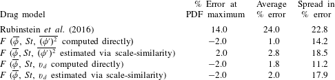
From figure 11 and table 4, the fact that all four inhomogeneous drag models have a very small bias
 $(\pm 3.0\,\%)$
confirms that we have properly fitted the simulation data with these new models over a full range of
 $\overline{\unicode[STIX]{x1D719}}$
and
 $St$
. While the error distributions are slightly skewed towards larger positive errors, this same conclusion can be made using either of the two measures for the model bias. In contrast, the Rubinstein et al. (Reference Rubinstein, Derksen and Sundaresan2016) model, on average, over-predicts the drag by
 $24.0\,\%$
due to the fact that this model was developed for homogeneous distributions of particles, and is therefore unable to account for the reduction in drag caused by inhomogeneities.
Since all four inhomogeneous drag models have essentially zero bias when predicting the drag for this particular set of LBM data, the key parameter in determining the utility of these models is the spread in the errors. Out of the four inhomogeneous models, the drift flux-dependent drag model, in which the drift flux is computed directly, has the smallest spread in the percentage error:
 $11.2\,\%$
. In comparison, the
 $\overline{(\unicode[STIX]{x1D719}^{\prime })^{2}}$
-dependent drag model, in which
 $\overline{(\unicode[STIX]{x1D719}^{\prime })^{2}}$
is computed directly, has a spread in the percentage error of
 $14.2\,\%$
. Thus, it is clear that if we are able to achieve a perfect estimation of these two subgrid quantities, the drift flux measure appears to provide a better fit for the drag force than the
 $\overline{(\unicode[STIX]{x1D719}^{\prime })^{2}}$
measure. From this analysis, it appears that incorporating the slip velocity into the measure for inhomogeneities provides a more powerful tool for modelling the drag than one that is solely based on the configuration of particles. Furthermore, in contrast with the homogeneous drag model of Rubinstein et al. (Reference Rubinstein, Derksen and Sundaresan2016), both of these new drag models are able to have a significantly smaller spread due to their ability to account for the effect of inhomogeneities.
From figure 4 and table 1, we observe that there is a modest increase in the spread in the prediction error when the subgrid quantities are estimated using a scale-similar approach with
 $\unicode[STIX]{x1D6E5}_{f,test}/d_{p}=5$
, rather than through a direct computation. Given this observed reduction in the model accuracy, it is clear that the scale-similar approach for estimating the subgrid quantities slightly degrades the quality of the drag force predictions. In particular, the fact that both models involving a scale-similar estimation have very similar spreads in the prediction error indicates that this effect is especially pronounced in the case of the drift flux scale-similar approach. Still, even when we use the scale-similar method to estimate the subfilter quantities, the spreads in the error predictions are still significantly smaller than for the Rubinstein et al. (Reference Rubinstein, Derksen and Sundaresan2016) case. This result further demonstrates that we have improved on the prior homogeneous drag models by accounting for the effect of subgrid-scale inhomogeneities.
From the results of this study, it is clear that the
 $\overline{(\unicode[STIX]{x1D719}^{\prime })^{2}}$
- and
 $v_{d}$
-based drag models each have their relative advantages and disadvantages. One of the main advantages of the drift flux measure is that, as seen in figure 11, if these subgrid-scale quantities can be directly computed, the
 $v_{d}$
-dependent drag model provides a more precise representation of the actual drag than the
 $\overline{(\unicode[STIX]{x1D719}^{\prime })^{2}}$
-dependent drag model. On the other hand, one of the main advantages for
 $\overline{(\unicode[STIX]{x1D719}^{\prime })^{2}}$
is that, as seen in figures 9(a) and 10(a),
 $\overline{(\unicode[STIX]{x1D719}^{\prime })^{2}}$
more strongly fits the scale-similarity approximation than does the drift flux. Due to this difference in the applicability of the scale-similar approach, in figure 11, the two inhomogeneous drag models are found to have almost identical precision when the subgrid-scale quantities are estimated using scale-similarity. In addition,
 $v_{d}$
is not only based on the configurations of particles, but also on the flow structures, which allows the drift flux to account for inhomogeneities in the slip velocity, whereas
 $\overline{(\unicode[STIX]{x1D719}^{\prime })^{2}}$
is only able to account for inhomogeneities in the particle distribution. However,
 $\overline{(\unicode[STIX]{x1D719}^{\prime })^{2}}$
has a simpler physical interpretation, as it is simply a measure of the fluctuations in the particle volume fraction, while the drift flux is a measure of the correlation between the slip velocity and the particle volume fraction. Based on this analysis, neither one of these options is definitively the better one, and so, instead, each of these two measures for the extent of subgrid-scale inhomogeneities should be considered in future studies of the effects of inhomogeneities on the drag.
Based on the observed increase in the spread of the drag prediction errors when employing the scale-similar approach, we see that there is some room for improvement in our modelling of the subgrid-scale inhomogeneities. One alternate technique for estimating these subgrid quantities is through the use of additional transport equations. Since these transport equations require additional constitutive closures, depending on the quality of these closures, this approach has the potential to improve the precision of our subgrid quantity estimation. Overall, the current work provides a promising approach for accounting for the effect of inhomogeneities on the fluid–particle drag force that can be further improved upon in future studies.
4 Summary
Through this work, using LBM simulations of fluidized beds with a cubic periodic domain analysed over a range of filter sizes, the effect of inhomogeneities on the fluid–particle drag force is quantified in the low-Re regime through one of two measures: the scalar variance of the particle volume fraction,
 $\overline{(\unicode[STIX]{x1D719}^{\prime })^{2}}$
, or the dimensionless drift flux,
 $v_{d}$
. Two new drag models (3.9) and (3.11) are then proposed that are, in addition to being functions of
 $\overline{\unicode[STIX]{x1D719}}$
and
 $St$
, dependent on one of these two measures for the extent of inhomogeneities. Unlike prior drag models that were derived under the assumption that the configuration of particles is randomly homogeneous, the newly proposed constitutive relations are able to account for the significant reduction in drag that occurs in the low-Re regime due to the presence of inhomogeneities.
By focusing on the low-Re regime, the current study is able to investigate the effects of inhomogeneities without the additional influences of inertial forces and granular temperature, which play a significant role at higher Re. A typical low-Re fluidized bed is one that is fluidized by ambient air, and whose particles have a diameter of
 $75~\unicode[STIX]{x03BC}\text{m}$
and a density of
 $1.5~\text{g}~\text{cm}^{-3}$
. While the terminal velocity of these particles is
 ${\sim}20~\text{cm}~\text{s}^{-1}$
, the minimum fluidization velocity is only approximately
 $4~\text{mm}~\text{s}^{-1}$
and the minimum bubbling velocity is approximately
 $2~\text{cm}~\text{s}^{-1}$
, which are both within the low-Re regime. While low-Re fluidized beds can exhibit both non-bubbling and bubbling behaviour, industrial fluidization processes typically involve faster flow velocities, and are therefore in the moderate-to-high-Re regime. However, even in industrial fluidized beds, the local fluid–particle slip velocities that govern the drag force are considerably smaller than the overall gas flow velocities. Having established the effects of inhomogeneities on the drag in the low-Re limit, the approach used in the current study can be utilized to extend this analysis to systems with higher Re. Higher-Re studies would provide insights into how the interplay between inhomogeneities, which tend to reduce the drag, and inertial forces and granular temperature, which tend to increase the drag, combine to affect the overall interactions between the fluid and particles.
The two identified measures for the extent of inhomogeneities,
 $\overline{(\unicode[STIX]{x1D719}^{\prime })^{2}}$
and
 $v_{d}$
, in our new drag models are both subgrid quantities. In contrast, the gradient in the volume fraction,
 $\unicode[STIX]{x1D735}\overline{\unicode[STIX]{x1D719}}$
, which was shown in prior studies to be a useful measure for the extent of inhomogeneities, is found to inadequately model the drag over a range of length scales due to its inability to account for subgrid-scale inhomogeneous structures. Thus, we have observed that the effect of inhomogeneities on the drag force are primarily tied to the extent of subgrid-scale inhomogeneities, as these are the structures that are not resolved at the scale at which the drag is computed.
An approach for estimating the subgrid measures is needed in order to utilize these subgrid-quantity-dependent drag relations in larger-scale simulations of fluidized beds, where the flow is not fully resolved. While the use of additional transport equations has the potential to provide higher accuracy in estimating these subgrid quantities, in this study, the subgrid quantities are estimated using a scale-similar approach, in which, based on the structures observed at a second, larger test filter size, the measure for the extent of inhomogeneities is extrapolated down to the
 $\unicode[STIX]{x1D6E5}_{f}$
-length scale. The scale-similar models for
 $\overline{(\unicode[STIX]{x1D719}^{\prime })^{2}}$
and
 $v_{d}$
are described by (3.14) and (3.23), respectively. Using these scale-similar approaches to estimate the subfilter quantities, both of the new drag models are shown to provide an improvement in the precision of the drag predictions over the prior homogeneous drag models.
While a direct quantitative comparison between the results in the current study and those of prior inhomogeneity studies cannot be made due to the fact these prior studies have not resulted in a generalized, low-Re constitutive drag relation, the key observed trends can, however, be compared. In these prior works (Zhou et al. Reference Zhou, Xiong, Wang, Wang, Ren and Ge2014; Li et al. Reference Li, Wang, Rogers, Zhou and Ge2017), the fluid–particle drag force is found to depend on both the direction and magnitude of the particle volume fraction gradient, with volume fraction gradients in the direction of the fluid–particle slip velocity causing an increase in drag, and volume fraction gradients perpendicular to the slip velocity causing a decrease in drag. In the current work, the drag force is found to depend only on the magnitude of the inhomogeneities, with increases in the inhomogeneities leading to a decrease in drag. Putting the results of the current work in the context of these prior studies, the effects of the volume fraction gradients perpendicular to the slip velocity significantly outweigh those of the parallel components. Overall, all of these inhomogeneity studies have identified the significant limitations in homogeneous drag relations due to their inability to account for inhomogeneities. The current work, however, is the first to propose a robust drag model that accounts for the effects of inhomogeneities over a full range of low-Re, dynamic fluidized beds.
In order to fully assess the effect of incorporating measures for the extent of inhomogeneities within the new drag constitutive relations, these new drag models must next be applied to larger-scale simulations of fluidized beds. In doing so, the differences between the fluidized bed behaviour predicted using these new drag relations and that using the prior homogeneous drag models will be ascertained, especially in relation to the grid resolution at which convergence in the flow behaviour is achieved, and to the flow structures that develop as a result of the fluid–particle interactions. Based on the strong effect of inhomogeneities on the fluid–particle drag force that we have demonstrated over the course of this study, the newly proposed drag models should provide a significant improvement over prior constitutive relations that fail to account for the extent of inhomogeneities.
Acknowledgements
This work is supported by a grant from the ExxonMobil Research & Engineering Co., and by a fellowship awarded to G.J.R. by the National Science Foundation (DGE-1148900).
Supplementary material
Supplementary material is available at https://doi.org/10.1017/jfm.2017.705.