1 Introduction
From the toroidal anti-dynamo theorem (Zel’dovich Reference Zel’dovich1957), we know that pure one-dimensional shear flows
 $\overline{\boldsymbol{U}}=f(y)\boldsymbol{e}_{x}$
can never be kinematic dynamos for any value of the magnetic Reynolds number
 $Rm$
(see (2.4)). Transient growth is possible but there can be no unbounded amplification of infinitesimal magnetic fields. But pure shear flows are too perfect to be real. Small perturbations
 $\boldsymbol{u}$
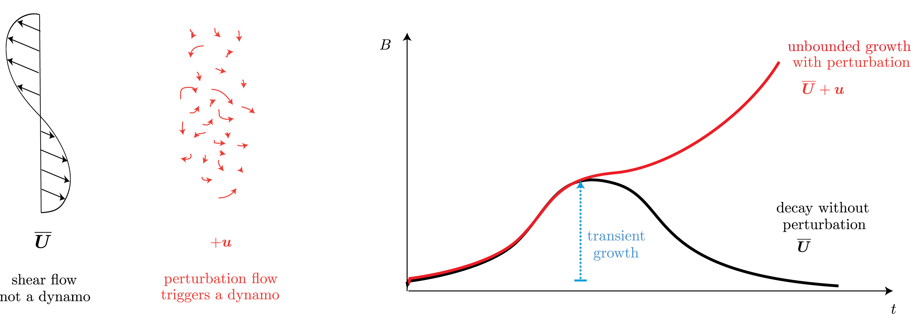
in the flow will always exist and from mean field dynamo theory (Braginsky Reference Braginsky1964; Moffatt Reference Moffatt1978; Krause & Rädler Reference Krause and Rädler1980) celebrated in this special issue, we know that such flow perturbations can trigger dynamo action (see sketch of figure 1). In this study, I measure the minimal magnitude of dynamo triggering flow perturbations as a function of
 $Rm$
and I provide theoretical elements that allow us to understand the optimal dynamo mechanism at high
 $Rm$
.
In earlier work on the same topic (Herreman (Reference Herreman2016), referred to as H16 hereafter), I used a variational optimization algorithm similar to Willis (Reference Willis2012), Chen, Herreman & Jackson (Reference Chen, Herreman and Jackson2015), Chen et al. (Reference Chen, Herreman, Li, Livermore, Luo and Jackson2018) to maximize kinematic dynamo action by the perturbed shear flow
 $\overline{\boldsymbol{U}}+\boldsymbol{u}$
. Kolmogorov flow
 $\overline{\boldsymbol{U}}=\sin y\,\boldsymbol{e}_{x}$
was fixed as an archetypical shear flow and the optimal perturbation
 $\boldsymbol{u}$
was sought within in the space of all three-dimensional stationary, solenoidal vector fields with square integrable vorticity. It is only recently that we know that large scale optimizations of this kind are numerically feasible (see recent review by Kerswell Reference Kerswell2018). The main result of H16 was that minimal flow perturbations need magnitudes
 $\boldsymbol{u}\sim Rm^{-1}$
to trigger a dynamo at magnetic Reynolds number
 $Rm$
. The minimal perturbation flow and the destabilized magnetic field both had simple spatial structures involving few Fourier modes in the
 $x$
and
 $z$
directions. Furthermore, the magnetic field mode aligned with the mean shear flow
 $\overline{\boldsymbol{U}}$
and had a weak streamwise dependence. This suggested that the optimal dynamo can be modelled as a mean field dynamo and this is what I do in this new study.
By truncating the flow perturbation and magnetic field to a set of well-chosen Fourier modes along
 $x$
and
 $z$
, the large scale optimization problem of H16 is transformed into a much simpler optimization problem, where only the
 $y$
-structure of the fields is left free to vary by the optimizer. The magnetic field evolution is constrained, not by the induction equation, but by a second-order mean field dynamo model. These reductions conserve the essence of the optimal dynamo of H16 and allow us to push the minimal flow perturbation study into the high
 $Rm$
regime that was previously inaccessible. Where
 $Rm=64$
was the highest explored value in H16, we can easily reach
 $Rm=10^{3}$
with this new approach, thus providing access to the asymptotically high
 $Rm$
-limit of the optimal dynamo.
In § 2 we define the problem and explain the optimization method that we have used. Section 3 gathers all the results. The new optimizations confirm the scaling law
 $\boldsymbol{u}\sim Rm^{-1}$
for the minimal magnitude of dynamo triggering flow perturbations. Intriguingly, we find that the rescaled optimal perturbation flow
 $\boldsymbol{v}=Rm\,\boldsymbol{u}$
is mainly independent of
 $Rm$
. In the high
 $Rm$
structure of the magnetic eigenmode, we find a critical layer phenomenon. In § 4, we identify the dynamo mechanism that seems to be of
 $\unicode[STIX]{x1D6FC}{-}\unicode[STIX]{x1D6FA}$
type and explain the origin of the critical layer. Section 5 concludes and discusses some connections with the problem of subcritical transition to turbulence.
In the kinematic dynamo approach, a one-dimensional shear flow
 $\overline{\boldsymbol{U}}$
can only transiently amplify magnetic field
 $\boldsymbol{B}$
. Well-chosen small perturbation flows can trigger unbounded growth of
 $\boldsymbol{B}$
. We measure the minimal magnitude of such dynamo triggering perturbations.

2 Methods
In an electrically conducting fluid with magnetic diffusivity
 $\unicode[STIX]{x1D702}_{\ast }$
, bounded by a periodical cube of size
 $L_{\ast }$
, we suppose a Kolmogorov shear flow
 $\overline{\boldsymbol{U}}_{\ast }=U_{\ast }\sin (2\unicode[STIX]{x03C0}y_{\ast }/L_{\ast })\,\boldsymbol{e}_{x}$
. Alone, this simple shear flow can never be a kinematic dynamo. We admit that the Kolmogorov flow is perturbed by stationary and solenoidal flow perturbations
 $\boldsymbol{u}_{\ast }$
with magnitude
 $$\begin{eqnarray}s_{\ast }=\sqrt{\frac{1}{{L_{\ast }}^{3}}\int (\unicode[STIX]{x1D735}_{\ast }\times \boldsymbol{u}_{\ast })^{2}\,\text{d}V_{\ast }}\end{eqnarray}$$
and we want to measure how small
 $s_{\ast }$
can minimally be, so that
 $\overline{\boldsymbol{U}}_{\ast }+\boldsymbol{u}_{\ast }$
is a kinematic dynamo. We non-dimensionalize the problem using
 $L_{\ast }/2\unicode[STIX]{x03C0}$
,
 $L_{\ast }/2\unicode[STIX]{x03C0}U_{\ast }$
,
 $U_{\ast }$
as length, time and velocity scales and denote all non-dimensional variables without stars.
In H16, I optimized the full three-dimensional spatial structure of the perturbation flow
 $\boldsymbol{u}(\boldsymbol{x})$
and the initial magnetic field
 $\boldsymbol{B}_{0}=\boldsymbol{B}(\boldsymbol{x},0)$
in order to maximize the logarithm of the magnetic field norm
 $$\begin{eqnarray}\ln \left(\frac{1}{8\unicode[STIX]{x03C0}^{3}}\int \boldsymbol{B}_{T}^{2}\,\text{d}V\right).\end{eqnarray}$$
Here
 $\boldsymbol{B}_{T}=\boldsymbol{B}(\boldsymbol{x},T)$
is the magnetic field at finite time
 $T$
. The evolution of
 $\boldsymbol{B}$
from time
 $t=0$
to
 $T$
was constrained by the induction equation and Gauss’ law:
 $$\begin{eqnarray}\unicode[STIX]{x2202}_{t}\boldsymbol{B}=\unicode[STIX]{x1D735}\times [(\overline{\boldsymbol{U}}+\boldsymbol{u})\times \boldsymbol{B}]+Rm^{-1}\unicode[STIX]{x0394}\boldsymbol{B},\quad \unicode[STIX]{x1D735}\boldsymbol{\cdot }\boldsymbol{B}=0.\end{eqnarray}$$
The magnetic Reynolds number was defined as
 $$\begin{eqnarray}Rm=\frac{U_{\ast }L_{\ast }}{2\unicode[STIX]{x03C0}\unicode[STIX]{x1D702}_{\ast }}.\end{eqnarray}$$
During the optimization, the flow
 $\boldsymbol{u}$
varies and all that is required is that it remains stationary, solenoidal
 $\unicode[STIX]{x1D735}\boldsymbol{\cdot }\boldsymbol{u}$
and that it conserves a non-dimensional perturbation magnitude
 $$\begin{eqnarray}s=\sqrt{\frac{1}{8\unicode[STIX]{x03C0}^{3}}\int (\unicode[STIX]{x1D735}\times \boldsymbol{u})^{2}\,\text{d}V}.\end{eqnarray}$$
Finally, it is necessary to normalize the initial magnetic field
 $$\begin{eqnarray}\frac{1}{8\unicode[STIX]{x03C0}^{3}}\int \boldsymbol{B}_{0}^{2}\,\text{d}V=1\end{eqnarray}$$
to have a well-defined optimization problem. The maximization objective and the mentioned physical constraints enter a Lagrangian functional
 $$\begin{eqnarray}\displaystyle {\mathcal{L}} & = & \displaystyle \ln \langle \boldsymbol{B}_{T}^{2}\rangle -\langle \unicode[STIX]{x1D6F1}_{1}\unicode[STIX]{x1D735}\boldsymbol{\cdot }\boldsymbol{u}\rangle -\unicode[STIX]{x1D706}_{1}(\langle (\unicode[STIX]{x1D735}\times \boldsymbol{u})^{2}\rangle -s^{2})\nonumber\\ \displaystyle & & \displaystyle -\,\langle \unicode[STIX]{x1D6F1}_{2}\unicode[STIX]{x1D735}\boldsymbol{\cdot }\boldsymbol{B}_{0}\rangle -\unicode[STIX]{x1D706}_{2}(\langle \boldsymbol{B}_{0}^{2}\rangle -1)\nonumber\\ \displaystyle & & \displaystyle -\int _{0}^{T}\langle \boldsymbol{B}^{\dagger }\boldsymbol{\cdot }[\unicode[STIX]{x2202}_{t}\boldsymbol{B}-\unicode[STIX]{x1D735}\times ((\overline{\boldsymbol{U}}+\boldsymbol{u})\times \boldsymbol{B})-Rm^{-1}\unicode[STIX]{x0394}\boldsymbol{B}]\rangle \,\text{d}t.\end{eqnarray}$$
We denote
 $\langle \cdots \rangle$
the volume average of the field and
 $\unicode[STIX]{x1D706}_{1},\unicode[STIX]{x1D706}_{2},\unicode[STIX]{x1D6F1}_{1},\unicode[STIX]{x1D6F1}_{2},\boldsymbol{B}^{\dagger }$
can be interpreted as Lagrange multipliers. Conditions for the optimal are derived by requiring that all variational derivatives need to vanish. This defines a big set of Euler–Lagrange equations that can be solved iteratively in an optimization loop. At each turn in the loop, direct (for
 $\boldsymbol{B}$
) and adjoint (for
 $\boldsymbol{B}^{\dagger }$
) induction equations are solved back and forward, after which the gradients
 $\unicode[STIX]{x1D6FF}{\mathcal{L}}/\unicode[STIX]{x1D6FF}\boldsymbol{u}$
and
 $\unicode[STIX]{x1D6FF}{\mathcal{L}}/\unicode[STIX]{x1D6FF}\boldsymbol{B}_{0}$
can be computed. These gradients serve to define updates for the flow
 $\boldsymbol{u}$
and
 $\boldsymbol{B}_{0}$
and they ultimately vanish as
 $\boldsymbol{u}$
and
 $\boldsymbol{B}_{0}$
converge towards an optimal. The algorithm can converge to local maxima so it is important to always launch several independent optimizations for the same parameter set. It is also important to use long time horizons
 $T\sim 3{-}4Rm$
in order to maximize the exponential growth of the fastest growing magnetic field eigenmode. This is crucial to separate unbounded amplification (kinematic dynamo) from just transient amplification (no kinematic dynamo). The optimization of the initial field structure
 $\boldsymbol{B}_{0}$
is only interesting because it allows us to use shorter
 $T$
.
In a systematic series of optimizations, H16 varied both
 $s$
and
 $Rm$
keeping
 $T=3Rm$
. For each optimized dynamo, one can measure the optimal dynamo growth rate
 $\unicode[STIX]{x1D6FE}$
as a function of
 $s$
and
 $Rm$
. Interpolation in this data set allows us to measure the minimal perturbation magnitude
 $s_{\text{min}}(Rm)$
as the magnitude
 $s$
for which
 $\unicode[STIX]{x1D6FE}(s_{\text{min}},Rm)=0$
, i.e. for which the optimal dynamo reached its threshold. This yielded the scaling law
 $s_{\text{min}}\sim Rm^{-1\pm 0.1}$
where the exponent was slightly unsure due to the numerical limitations. Full three-dimensional optimizations are rather costly and this explains why the moderate value of
 $Rm=64$
was the highest explored value in H16.
In the present study, we overcome the limitations on
 $Rm$
by reformulating the three-dimensional optimization problem of H16 as a much lighter, one-dimensional optimization problem. We exploit the fact that the minimal flow perturbation
 $\boldsymbol{u}$
and the magnetic eigenmode
 $\boldsymbol{B}$
found by H16 had relatively simple spatial structures, involving few Fourier modes in the
 $x$
(streamwise) and
 $z$
(spanwise) directions. Rather than optimizing the full three-dimensional structure of the perturbation flows, we limit the search space to
 $$\begin{eqnarray}\boldsymbol{u}=\overline{\boldsymbol{u}}(y)+\underbrace{\{\boldsymbol{w}(y)+[\boldsymbol{w}_{+}(y)\text{e}^{\text{i}2z}+\boldsymbol{w}_{-}(y)\text{e}^{-\text{i}2z}]\}\text{e}^{\text{i}x}+\text{c.c.}}_{\boldsymbol{u}^{\prime }(x,y,z)}\end{eqnarray}$$
with
 $\unicode[STIX]{x1D735}\boldsymbol{\cdot }\boldsymbol{u}=0$
. These four modes really dominated the structure in the optimal flow perturbation of H16, so we can expect decent results with this severe truncation. Here and elsewhere, the overline stands for
 $x$
-independent (mean) part and primes for the
 $x$
-dependent (fluctuation) part. c.c. stands for complex conjugate. The spatial profiles
 $\overline{\boldsymbol{u}}(y),\boldsymbol{w}(y),\boldsymbol{w}_{\pm }(y)$
are left free to vary by the optimization algorithm, but just as in H16, we need to fix a normalization to the space of functions. With
 $$\begin{eqnarray}s=\sqrt{\langle \Vert \unicode[STIX]{x1D735}_{\!0,0}\times \overline{\boldsymbol{u}}\Vert ^{2}\rangle +2\langle \Vert \unicode[STIX]{x1D735}_{\!1,0}\times \boldsymbol{ w}\Vert ^{2}\rangle +2\langle \Vert \unicode[STIX]{x1D735}_{\!1,2}\times \boldsymbol{ w}_{+}\Vert ^{2}\rangle +2\langle \Vert \unicode[STIX]{x1D735}_{\!1,-2}\times \boldsymbol{ w}_{-}\Vert ^{2}\rangle }\end{eqnarray}$$
and
 $\langle \cdots \rangle =(1/2\unicode[STIX]{x03C0})\int _{0}^{2\unicode[STIX]{x03C0}}\ldots \,\text{d}y$
we use the same normalization as in H16. We denote
 $\unicode[STIX]{x1D735}_{\!m,n}=m\,\boldsymbol{e}_{x}+\boldsymbol{e}_{y}\,\unicode[STIX]{x2202}_{y}+n\,\boldsymbol{e}_{z}$
. For the magnetic field, we similarly truncate to a restricted functional space
 $$\begin{eqnarray}\boldsymbol{B}=\underbrace{\overline{\boldsymbol{b}}(y,t)\text{e}^{\text{i}z}+\text{c.c.}}_{\overline{\boldsymbol{B}}(y,z,t)}+\underbrace{[\boldsymbol{b}_{+}(y,t)\text{e}^{\text{i}z}+\boldsymbol{b}_{-}(y,t)\text{e}^{-\text{i}z}]\boldsymbol{e}^{\text{i}x}+\text{c.c.}}_{\boldsymbol{B}^{\prime }(x,y,z,t)}+\cdots\end{eqnarray}$$
with
 $\unicode[STIX]{x1D735}\boldsymbol{\cdot }\boldsymbol{B}=0$
. In the optimal dynamo of H16, these three modes also dominate and the
 $x$
-independent field
 $\overline{\boldsymbol{B}}$
was much larger than the
 $x$
-dependent part
 $\boldsymbol{B}^{\prime }$
. This means that we can constrain the magnetic field evolution, not by the induction equation but by a second-order mean field model. The usual equations for such model are
 $$\begin{eqnarray}\displaystyle & \displaystyle \unicode[STIX]{x2202}_{t}\overline{\boldsymbol{B}}=\unicode[STIX]{x1D735}\times [(\overline{\boldsymbol{U}}+\overline{\boldsymbol{u}})\times \overline{\boldsymbol{B}}]+\unicode[STIX]{x1D735}\times \overline{(\boldsymbol{u}^{\prime }\times \boldsymbol{B}^{\prime })}+Rm^{-1}\unicode[STIX]{x0394}\overline{\boldsymbol{B}} & \displaystyle\end{eqnarray}$$
 $$\begin{eqnarray}\displaystyle & \displaystyle \unicode[STIX]{x2202}_{t}\boldsymbol{B}^{\prime }=\unicode[STIX]{x1D735}\times [(\overline{\boldsymbol{U}}+\overline{\boldsymbol{u}})\times \boldsymbol{B}^{\prime }]+\unicode[STIX]{x1D735}\times (\boldsymbol{u}^{\prime }\times \overline{\boldsymbol{B}})+Rm^{-1}\unicode[STIX]{x0394}\boldsymbol{B}^{\prime }+\cdots & \displaystyle\end{eqnarray}$$
 $$\begin{eqnarray}\displaystyle & \displaystyle \unicode[STIX]{x2202}_{t}\overline{\boldsymbol{b}}=\unicode[STIX]{x1D735}_{\!0,1}\times [(\overline{\boldsymbol{U}}+\overline{\boldsymbol{w}})\times \overline{\boldsymbol{b}}+\boldsymbol{w}\times \boldsymbol{b}_{-}^{\ast }+\boldsymbol{w}^{\ast }\times \boldsymbol{b}_{+}+\boldsymbol{w}_{+}\times \boldsymbol{b}_{+}^{\ast }+\boldsymbol{w}_{-}^{\ast }\times \boldsymbol{b}_{-}]+Rm^{-1}\unicode[STIX]{x1D6FB}_{0,1}^{2}\overline{\boldsymbol{b}} & \displaystyle \nonumber\\ \displaystyle & & \displaystyle\end{eqnarray}$$
 $$\begin{eqnarray}\displaystyle & \unicode[STIX]{x2202}_{t}\boldsymbol{b}_{+}=\unicode[STIX]{x1D735}_{\!1,1}\times [(\overline{\boldsymbol{U}}+\overline{\boldsymbol{w}})\times \boldsymbol{b}_{+}+\boldsymbol{w}\times \overline{\boldsymbol{b}}+\boldsymbol{w}_{+}\times \overline{\boldsymbol{b}}^{\ast }]+Rm^{-1}\unicode[STIX]{x1D6FB}_{1,1}^{2}\boldsymbol{b}_{+} & \displaystyle\end{eqnarray}$$
 $$\begin{eqnarray}\displaystyle & \unicode[STIX]{x2202}_{t}\boldsymbol{b}_{-}=\unicode[STIX]{x1D735}_{\!1,-1}\times [(\overline{\boldsymbol{U}}+\overline{\boldsymbol{w}})\times \boldsymbol{b}_{-}+\boldsymbol{w}\times \overline{\boldsymbol{b}}^{\ast }+\boldsymbol{w}_{-}\times \overline{\boldsymbol{b}}]+Rm^{-1}\unicode[STIX]{x1D6FB}_{1,-1}^{2}\boldsymbol{b}_{-} & \displaystyle\end{eqnarray}$$
 $\overline{\boldsymbol{b}}(y,0),\boldsymbol{b}_{\pm }(y,0)$
and normalize them as
 $$\begin{eqnarray}1=2\langle \overline{\boldsymbol{b}}^{2}(y,0)\rangle +2\langle \boldsymbol{b}_{+}^{2}(y,0)\rangle +2\langle \boldsymbol{b}_{-}^{2}(y,0)\rangle .\end{eqnarray}$$
Finally, we keep the same the maximization objective, changing
 $\ln \langle \boldsymbol{B}_{T}^{2}\rangle$
of (2.7) into
 $$\begin{eqnarray}\ln \underbrace{(2\langle \overline{\boldsymbol{b}}^{2}(y,T)\rangle +2\langle \boldsymbol{b}_{+}^{2}(y,T)\rangle +2\langle \boldsymbol{b}_{-}^{2}(y,T)\rangle )}_{E_{T}}.\end{eqnarray}$$
In the Appendix we provide further details on the Lagrangian functional
 ${\mathcal{L}}$
that replaces (2.7) but is too long to write here. This new
 ${\mathcal{L}}$
sets the starting point for our iterative algorithm and optimality conditions are deduced as usual. Since there are more variables than in H16, it is slightly more laborious to manipulate the equations, but apart from that, there are no particular difficulties. We spectrally decompose the
 $y$
-structure of the fields on a Fourier basis and use the same numerical schemes as in H16 to time step direct and adjoint equations and to define updates.
In practice, we initialize the optimization loop with random
 $\boldsymbol{u}$
and
 $\boldsymbol{B}_{0}$
and converge all optima up to an optimization error of
 $r_{i}\leqslant 10^{-3}$
(defined as in H16) or alternatively, up until
 $E_{T}$
varies by less than
 $10^{-8}$
between two successive iterations. We fix the final time to
 $T=4Rm$
and once an optimum is found, we integrate the induction equation once with the optimal configuration up to the time
 $T=16Rm$
. An exponential fit on
 $E_{T}$
over the time lapse
 $t\in [12Rm,16Rm]$
allows us to measure the optimal dynamo growth rate
 $\unicode[STIX]{x1D6FE}$
with high precision.
Due to the symmetries of the Kolmogorov flow, optimal configurations are degenerate. We introduce a change in coordinates
 $\check{\boldsymbol{x}}=\boldsymbol{x}_{0}+{\mathcal{R}}\boldsymbol{x}$
with
 $$\begin{eqnarray}\boldsymbol{x}_{0}=\left[\begin{array}{@{}c@{}}a\\ \unicode[STIX]{x03C0}\unicode[STIX]{x1D6FF}\\ c\end{array}\right],\quad {\mathcal{R}}=\left[\begin{array}{@{}ccc@{}}s_{1} & & \\ & s_{2} & \\ & & s_{3}\end{array}\right]\end{eqnarray}$$
and
 $\unicode[STIX]{x1D6FF}=0,1$
,
 $a,c\in [\!0,2\unicode[STIX]{x03C0}\ $s_{j}=-1,1$
. Note that
 ${\mathcal{R}}^{2}={\mathcal{I}}$
. Kolmogorov flow is (anti-) symmetrical with respect to such coordinate changes and we can write a general formula
 $$\begin{eqnarray}\overline{\boldsymbol{U}}(\boldsymbol{x})=\underbrace{s_{1}s_{2}(-1)^{\unicode[STIX]{x1D6FF}}}_{S}{\mathcal{R}}\overline{\boldsymbol{U}}({\mathcal{R}}\boldsymbol{x}).\end{eqnarray}$$
For all symmetry transforms
 $(S=1)$
, it is easy to show that the Lagrangian remains invariant provided that we transform flow perturbations and magnetic fields as
 $$\begin{eqnarray}\check{\boldsymbol{u}}(\boldsymbol{x})={\mathcal{R}}\boldsymbol{u}({\mathcal{R}}(\boldsymbol{x}-\boldsymbol{x}_{0})),\quad \check{\boldsymbol{B}}(\boldsymbol{x},t)={\mathcal{R}}\boldsymbol{B}({\mathcal{R}}(\boldsymbol{x}-\boldsymbol{x}_{0}),t),\ldots\end{eqnarray}$$
These relations were needed to do a meaningful comparison of independently obtained optima. In practice, optimal field configurations are translated, rotated and reflected to a reference optimum for which we fix
 $w_{z}$
to be maximal and rea l in the middle of the computational domain (
 $y=\unicode[STIX]{x03C0}$
),
 $\arg (w_{+,y}(\unicode[STIX]{x03C0}))=\arg (w_{-,y}(\unicode[STIX]{x03C0}))$
and
 $\text{Im}(w_{+,y}(\unicode[STIX]{x03C0}))>0$
.
3 Results
As in H16, I performed a systematic series of optimizations varying both parameters,
 $s$
and
 $Rm$
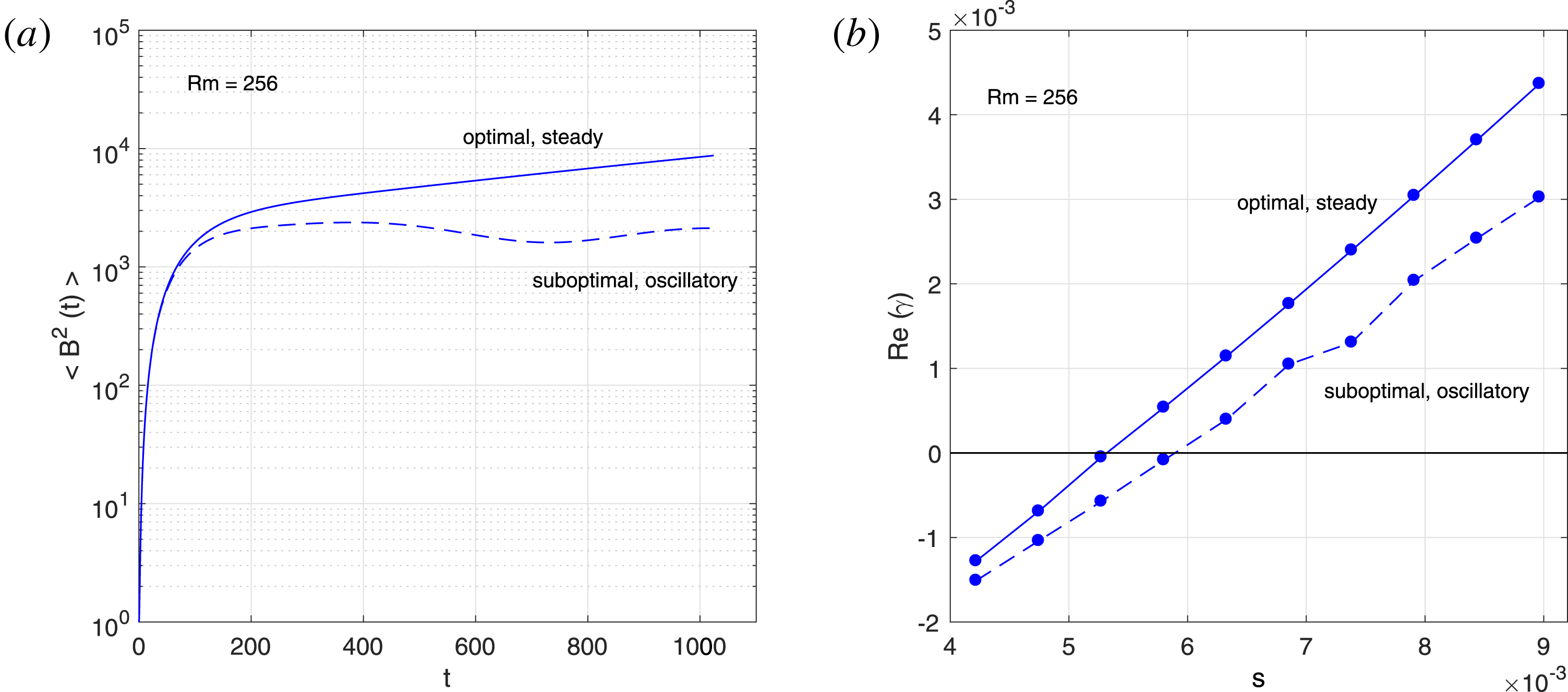
. For each parameter set several (6–12) independent optimizations were done, starting from different random initial configurations. As shown in figure 2, the algorithm can converge to steady dynamo states (
 $\text{Im}(\unicode[STIX]{x1D6FE})=0$
) or to suboptimal states that correspond to oscillatory dynamos (
 $\text{Im}(\unicode[STIX]{x1D6FE})\neq 0$
). Suboptimal branches were only sporadically seen in the three-dimensional optimizations of H16 but are more frequently observed in this mean field model. From now on, we focus on the optimal dynamo branch that is steady.
The optimization algorithm converges to either an optimal or a suboptimal branch. In (a), we see that the optimal dynamo is always a steady dynamo, whereas the suboptimal branch is an oscillatory dynamo (
 $Rm=256$
,
 $s=5.8\times 10^{-3}$
). In (b), we compare growth rate measures
 $Re(\unicode[STIX]{x1D6FE})$
of both optimal and suboptimal branches for various values of
 $s$
.

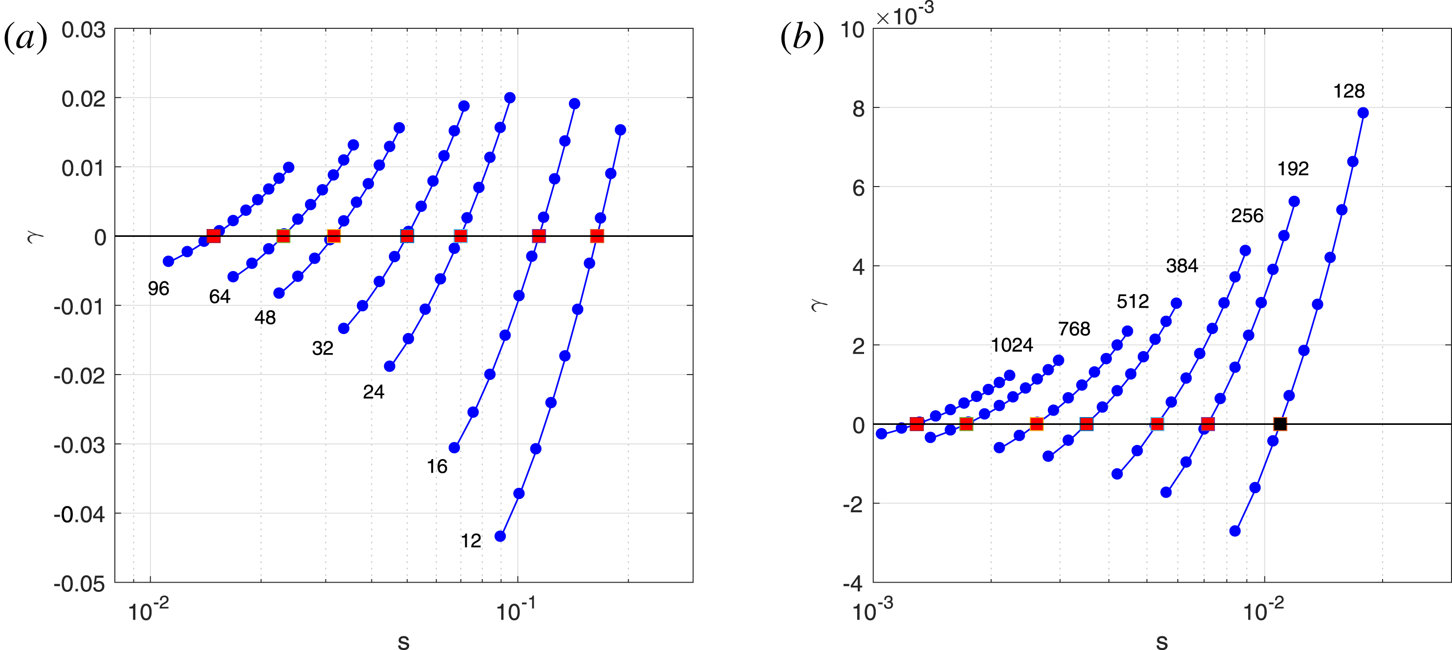
3.1 Optimal growth rates and minimal magnitudes
Optimal growth rates
 $\unicode[STIX]{x1D6FE}(s,Rm)$
as a function of perturbation magnitude
 $s$
and for various
 $Rm$
as marked in the figure.

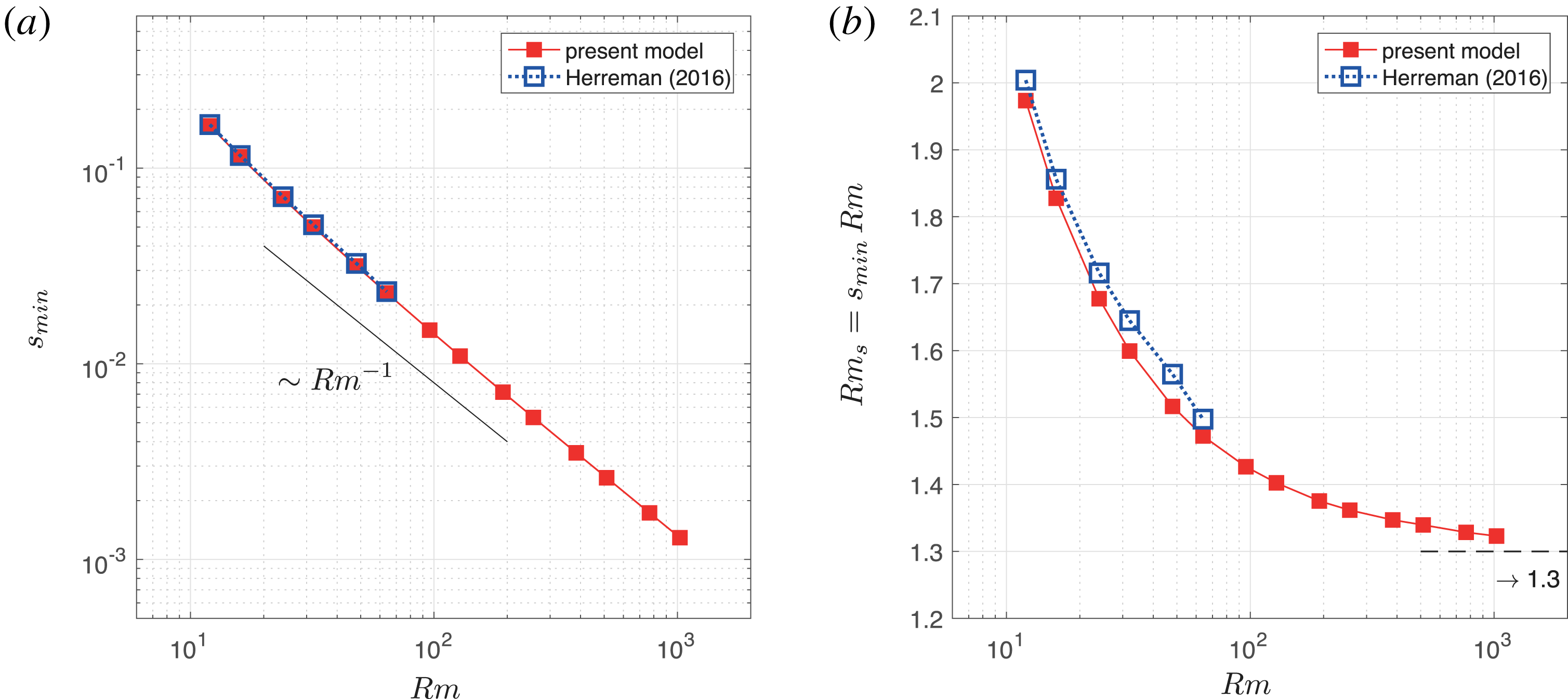
(a) From the optimal growth rate data, we interpolate minimal perturbation magnitudes
 $s_{\text{min}}(Rm)$
and plot them a function of
 $Rm$
. Our new data points align with the data of H16 and the scaling law
 $s_{\text{min}}\sim Rm^{-1}$
is clearly visible. (b) By plotting the rescaled magnetic Reynolds number
 $Rm_{s,\text{min}}=s_{\text{min}}Rm$
as a function of
 $Rm$
we can make a finer comparison. Notice how an asymptotic value
 $Rm_{s,\text{min}}\rightarrow 1.3$
is reached in the high
 $Rm$
limit.

In figure 3 we show the optimal dynamo growth rates
 $\unicode[STIX]{x1D6FE}$
as a function of
 $s$
. Data points are gathered per value of
 $Rm$
as marked in the figure. Per group of
 $Rm$
, we see that the optimal growth rates increase monotonically with perturbation magnitude
 $s$
. From these data, we can interpolate the minimal perturbation magnitudes
 $s_{\text{min}}(Rm)$
at which the optimal dynamo reaches its threshold (data points marked with red squares). Numerical measures are given in table 1 and they are plotted as a function of
 $Rm$
in figure 4(a). The new mean field data points superpose with the data points of H16 and from moderate to high
 $Rm$
, we now clearly observe a scaling law
 $$\begin{eqnarray}s_{\text{min}}\sim Rm^{-1}\end{eqnarray}$$
that was suggested in H16. This scaling law can be reformulated more simply as a lower bound on the perturbation flow magnetic Reynolds number
 $$\begin{eqnarray}Rm_{s}=sRm=\frac{s_{\ast }L_{\ast }^{2}}{4\unicode[STIX]{x03C0}^{2}\unicode[STIX]{x1D702}_{\ast }}.\end{eqnarray}$$
Perturbations
 $\boldsymbol{u}$
in the explored class of functions can only trigger dynamos in Kolmogorov flow when
 $$\begin{eqnarray}Rm_{s}>Rm_{s,\text{min}}\quad \text{with}\quad Rm_{s,\text{min}}=s_{\text{min}}Rm.\end{eqnarray}$$
In figure 4(b), we plot
 $Rm_{s,\text{min}}$
as a function of
 $Rm$
. We clearly observe a high
 $Rm$
-limit (see also table 1) in which
 $$\begin{eqnarray}\lim _{Rm\rightarrow +\infty }Rm_{s,\text{min}}\approx 1.3\pm 0.1.\end{eqnarray}$$
Mainly
 $Rm_{s}$
decides whether there can be a kinematic dynamo or not in the perturbed Kolmogorov flow, the precise value of
 $Rm$
is less important, provided that it is high enough.
Minimal perturbation shear magnitudes
 $s_{\text{min}}$
as a function of
 $Rm$
. The rescaled magnetic Reynolds number
 $Rm_{s,\text{min}}=s_{\text{min}}Rm$
reaches towards an asymptote estimated near
 $Rm_{s,\text{min}}\rightarrow 1.3\pm 0.01$
.

3.2 Spatial structure of the minimal flow perturbation
We compute optimal configurations for parameters
 $(s,Rm)=(s_{\text{min}}(Rm),Rm)$
of table 1 at the optimal dynamo threshold (
 $\unicode[STIX]{x1D6FE}=0$
). With the mentioned phase convention, we find a reference optimal state for which we always have
 $$\begin{eqnarray}\overline{u}_{x},\overline{u}_{z},w_{x},w_{z},w_{\pm ,x},w_{\pm ,z}\in \mathbb{R},\quad w_{y},w_{\pm ,y}\in \text{i}\mathbb{R}\end{eqnarray}$$
and
 $\overline{u}_{y}=0$
. The
 $y$
-structure of the flow components renormalized by
 $s$
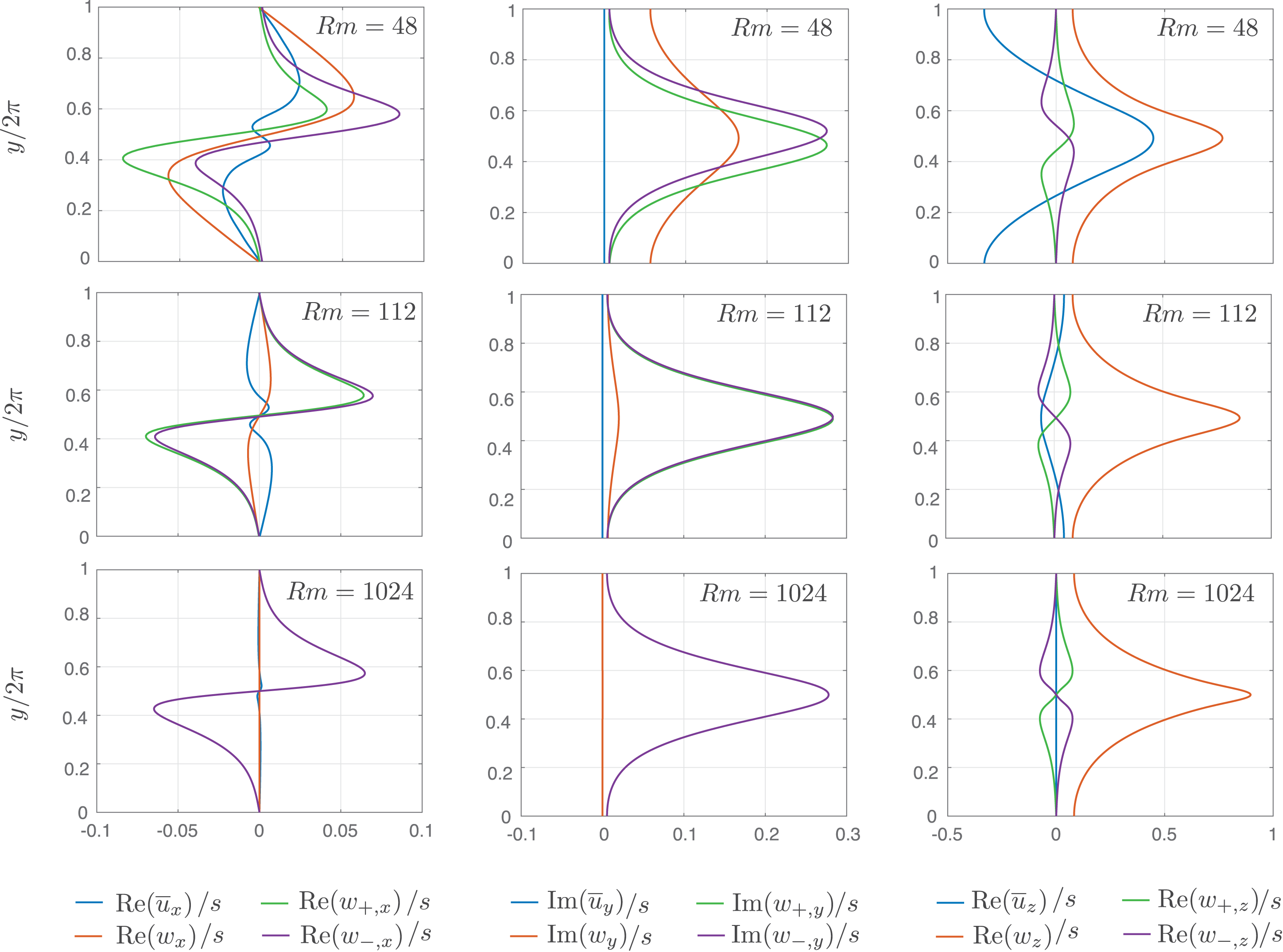
, is plotted in figure 5, for low, intermediate and high
 $Rm=48$
, 112, 1024. At low
 $Rm$
there is a mean flow modification
 $\overline{\boldsymbol{u}}\neq \mathbf{0}$
as in H16. In the interval
 $Rm\in [60,130]$
, we see that the mean flow component gradually vanishes, but it is necessary to mention that this figure for
 $Rm=112$
is slightly uncertain. For
 $Rm\in [60,130]$
, the optimizer does not converge to a well-defined state with or without small mean flow. Small
 $\overline{\boldsymbol{u}}$
apparently does not affect the magnetic field amplification in a significant way. At high
 $Rm$
, we find that the optimal flow has a much simpler spatial structure without mean flow
 $\overline{\boldsymbol{u}}\approx \mathbf{0}$
and with
 $\boldsymbol{w}\approx w_{z}(y)\boldsymbol{e}_{z}$
and
 $w_{+,x}\approx w_{-,x}$
,
 $w_{+,y}\approx w_{-,x}$
,
 $w_{+,z}\approx -w_{-,z}$
. Combined with (3.5) and (2.8) this suggests an asymptotic, high
 $Rm$
optimal perturbation flow of the type
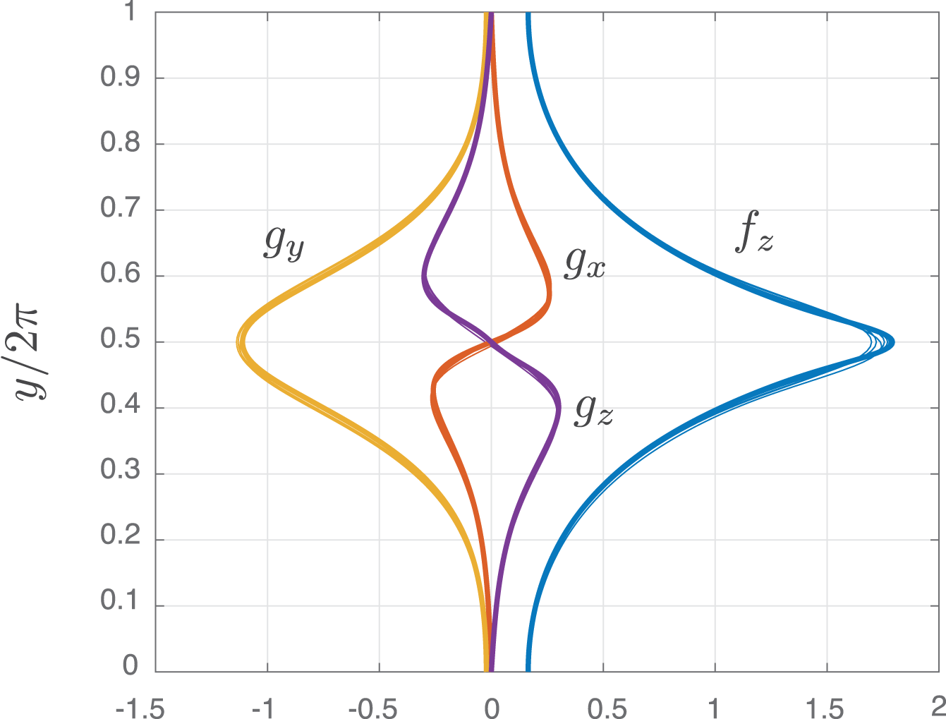
 $$\begin{eqnarray}\displaystyle \left[\begin{array}{@{}c@{}}u_{x}/s\\ u_{y}/s\\ u_{z}/s\end{array}\right]=\left[\begin{array}{@{}c@{}}0\\ 0\\ f_{z}(y)\cos x\end{array}\right]+\left[\begin{array}{@{}c@{}}g_{x}(y)\cos x\cos 2z\\ g_{y}(y)\sin x\cos 2z\\ g_{z}(y)\sin x\sin 2z\end{array}\right]. & & \displaystyle\end{eqnarray}$$
The profiles
 $f(y),g_{x}(y),g_{y}(y),g_{z}(y)$
are shown in figure 6, for various
 $Rm\in [128,1024]$
. The optimal perturbation flow renormalized by
 $s$
has a spatial structure that is mostly independent of
 $Rm$
at high
 $Rm$
.
Spatial profiles of the components of
 $\overline{\boldsymbol{u}}(y),\boldsymbol{w}(y),\boldsymbol{w}_{\pm }(y)$
that define the minimal perturbation flow
 $\boldsymbol{u}$
(see (2.8)). At low
 $Rm=48$
, the optimal perturbation flow is more complex and there is a mean flow perturbation
 $\overline{\boldsymbol{u}}\neq 0$
. At high
 $Rm=1024$
,
 $\boldsymbol{u}$
is simpler, since
 $\overline{\boldsymbol{u}}\approx \mathbf{0}$
,
 $\boldsymbol{w}\approx w_{z}\boldsymbol{e}_{z}$
and
 $\boldsymbol{w}_{\pm }$
are strongly correlated. In an intermediate range of
 $Rm\in [60,130]$
, we observe a passage between the low and high
 $Rm$
states.

The minimal perturbation flow renormalized by
 $s$
(or
 $Rm$
) is mainly independent of
 $Rm$
at high
 $Rm$
. Here we cumulate profiles
 $f_{z}(y)$
,
 $g_{x}(y)$
,
 $g_{y}(y)$
,
 $g_{z}(y)$
that appear in the simplified formula (3.6) for
 $\boldsymbol{u}/s$
, for various higher
 $Rm=128\rightarrow 1024$
.

3.3 Spatial structure of the magnetic field
To compare magnetic field eigenmodes for different
 $Rm$
, we rescale
 $\boldsymbol{B}_{T}$
by the final time norm
 $\sqrt{E_{T}}$
and we choose the sign of
 $\boldsymbol{B}$
so that
 $\overline{b}_{x}(\unicode[STIX]{x03C0})>0$
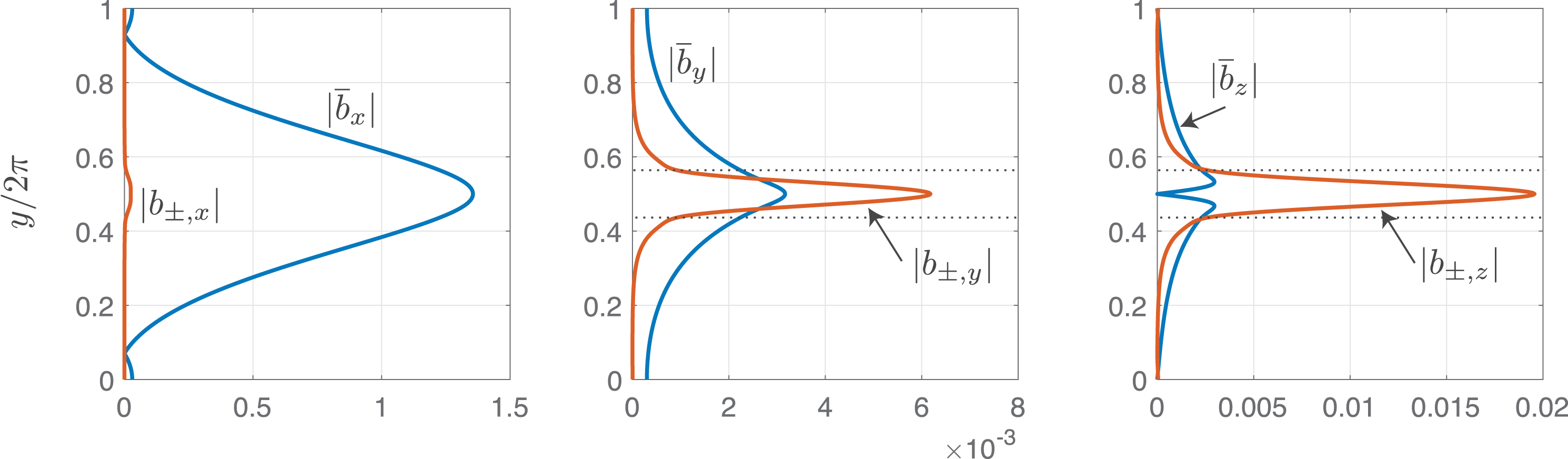
. Figure 7 shows a typical profile that is observed for high
 $Rm=1024$
. Clearly, the streamwise ‘mean’ component
 $\overline{b}_{x}$
is much larger than all other field components: the magnetic field almost aligns with the mean flow at high
 $Rm$
. Fields
 $\boldsymbol{b}_{\pm }$
are smaller as they should and seem to localize near
 $y=\unicode[STIX]{x03C0}$
. The field components
 $\overline{b}_{y},\overline{b}_{z}$
are the smallest and they are not as localized.
Spatial structure of the magnetic field modes
 $\overline{\boldsymbol{b}}(y),\boldsymbol{b}_{\pm }(y)$
at high
 $Rm=1024$
. The mean magnetic field
 $\overline{\boldsymbol{b}}$
really is dominated by a strong
 $x$
-component and is not localized. The fields
 $\boldsymbol{b}_{\pm }(y)$
are much smaller and localized near the
 $y=\unicode[STIX]{x03C0}$
shear layer (suggested by dashed lines).

The different magnetic field variables vary differently with
 $Rm$
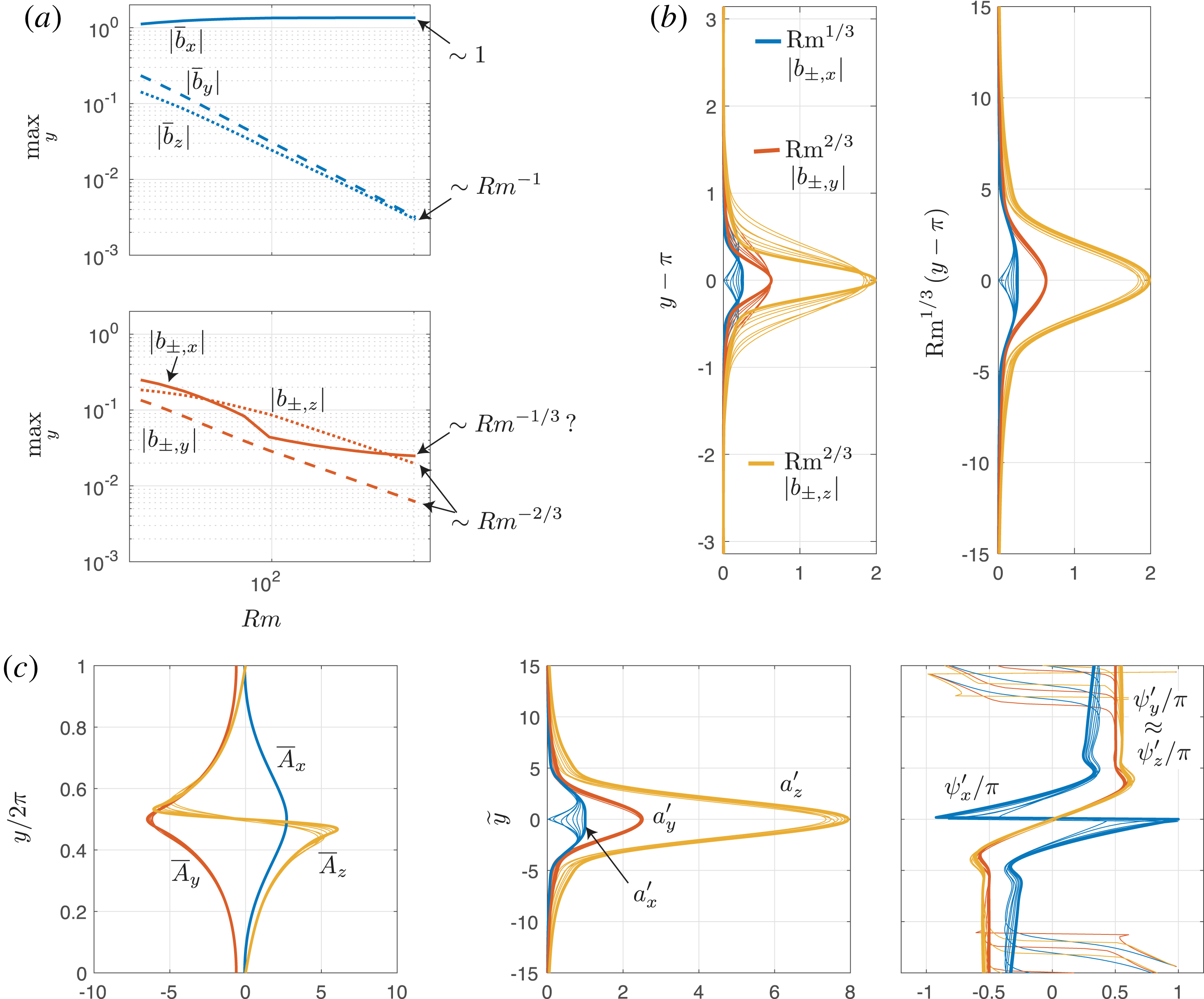
. The maximal absolute values of the components of
 $\overline{\boldsymbol{b}}(y)$
and
 $\boldsymbol{b}_{\pm }(y)$
are plotted as a function of
 $Rm$
in figure 8(a). This suggests power-law behaviour
 $$\begin{eqnarray}\left.\begin{array}{@{}l@{}}\overline{b}_{x}\sim 1\\ \overline{b}_{y}\sim Rm^{-1}\\ \overline{b}_{z}\sim Rm^{-1}\end{array}\right\},\quad \left.\begin{array}{@{}l@{}}b_{\pm ,x}\sim Rm^{-1/3~?}\\ b_{\pm ,y}\sim Rm^{-2/3}\\ b_{\pm ,z}\sim Rm^{-2/3}.\end{array}\right\}\end{eqnarray}$$
All laws are well established except for
 $b_{\pm ,x}\sim Rm^{-1/3}$
that is not observed. Below I provide arguments in favour of this scaling law. In figure 8(b), it is demonstrated that the magnetic field
 $\boldsymbol{b}_{\pm }$
localizes in
 $Rm^{-1/3}$
wide layers. The left panel groups the original field components rescaled in magnitude for different
 $Rm$
plotting them versus
 $y-\unicode[STIX]{x03C0}$
. There is little are no alignment in the different profiles. In the right panel, the same profiles are shown, this time as a function of the zoomed variable
 $$\begin{eqnarray}{\tilde{y}}=Rm^{1/3}(y-\unicode[STIX]{x03C0}).\end{eqnarray}$$
This scaling law seems rather well adapted to align all the different high
 $Rm$
profiles. This kind of localization in
 $O(Rm^{-1/3})$
-wide layers is typical for diffusive critical layers (see for example Drazin & Reid Reference Drazin and Reid2004). A phase shift of
 $\unicode[STIX]{x03C0}/4$
simplifies the interpretation of the magnetic field profiles since
 $$\begin{eqnarray}\overline{b}_{x}\text{e}^{\text{i}\unicode[STIX]{x03C0}/4},\quad \overline{b}_{y}\text{e}^{\text{i}\unicode[STIX]{x03C0}/4}\in \mathbb{R},\quad \overline{b}_{z}\text{e}^{\text{i}\unicode[STIX]{x03C0}/4}\in \text{i}\mathbb{R},\quad \text{Re}(b_{+,z}\text{e}^{\text{i}\unicode[STIX]{x03C0}/4})=-\text{Im}(b_{-,z}\text{e}^{\text{i}\unicode[STIX]{x03C0}/4}),\ldots\end{eqnarray}$$
This information together with that for the scalings of the magnitudes and considering the initial truncation (2.10) brings us to a simplified formula for the asymptotic high
 $Rm$
magnetic field mode:
 $$\begin{eqnarray}\left[\begin{array}{@{}c@{}}\overline{B}_{x}\\ \overline{B}_{y}\\ \overline{B}_{z}\end{array}\right]=\left[\begin{array}{@{}c@{}}\overline{A}_{x}(y)\cos (z-\unicode[STIX]{x03C0}/4)\\ Rm^{-1}\,\overline{A}_{y}(y)\cos (z-\unicode[STIX]{x03C0}/4)\\ Rm^{-1}\,\overline{A}_{z}(y)\sin (z-\unicode[STIX]{x03C0}/4)\end{array}\right]\end{eqnarray}$$
and
 $$\begin{eqnarray}\left[\begin{array}{@{}c@{}}b_{x}^{\prime }\\ b_{y}^{\prime }\\ b_{z}^{\prime }\end{array}\right]=\left[\begin{array}{@{}c@{}}Rm^{-1/3}a_{x}^{\prime }(\,\widetilde{y}\,)\sin (x+\unicode[STIX]{x1D713}_{x}^{\prime }(\,\widetilde{y}\,))\cos (z-\unicode[STIX]{x03C0}/4)\\ Rm^{-2/3}a_{y}^{\prime }(\,\widetilde{y}\,)\sin (x+\unicode[STIX]{x1D713}_{y}^{\prime }(\,\widetilde{y}\,))\cos (z-\unicode[STIX]{x03C0}/4)\\ Rm^{-2/3}a_{z}^{\prime }(\,\widetilde{y}\,)\cos (x+\unicode[STIX]{x1D713}_{z}^{\prime }(\,\widetilde{y}\,))\sin (z-\unicode[STIX]{x03C0}/4)\end{array}\right].\end{eqnarray}$$
Figure 8(c) displays all high
 $Rm$
profiles of
 $\overline{A}_{j}(y),a_{j}^{\prime }(\,\widetilde{y}\,),\unicode[STIX]{x1D713}_{j}^{\prime }(\,\widetilde{y}\,)$
for
 $j=x,y,z$
. All the optimal fields align reasonably well. Note that
 $\overline{A}_{z}$
changes sign abruptly, probably in the
 $O(Rm^{-1/3})$
area around
 $y=\unicode[STIX]{x03C0}$
. Notice also the proportionality
 $a_{y}^{\prime }(\,\widetilde{y}\,)\sim a_{z}^{\prime }(\,\widetilde{y}\,)$
and the nearly linear phase slips in
 $$\begin{eqnarray}\unicode[STIX]{x1D713}_{y}^{\prime }(\,\widetilde{y}\,)\approx \unicode[STIX]{x1D713}_{z}^{\prime }(\,\widetilde{y}\,)\approx 4.5\widetilde{y}\end{eqnarray}$$
and a jump from
 $-\unicode[STIX]{x03C0}/2$
to
 $\unicode[STIX]{x03C0}/2$
as we pass
 $\widetilde{y}=-5\rightarrow +5$
. The phase
 $\unicode[STIX]{x1D713}_{x}^{\prime }(\,\widetilde{y}\,)$
makes a slip that is three times larger, from nearly
 $-\unicode[STIX]{x03C0}/4\rightarrow \unicode[STIX]{x03C0}$
for negative
 $\widetilde{y}$
and from
 $-\unicode[STIX]{x03C0}\rightarrow \unicode[STIX]{x03C0}/4$
for positive
 $\widetilde{y}$
in a similar
 $\widetilde{y}$
-interval. The strange behaviour of the phase curves when
 $|\widetilde{y}|\gg 5$
is irrelevant since the field
 $\boldsymbol{b}^{\prime }$
becomes too small there.
Magnetic field structure and magnitude for varying
 $Rm$
. (a) Scaling of the maximal values of the different magnetic field components as a function of
 $Rm$
. (b) Localization of
 $\boldsymbol{b}_{\pm }$
in
 $Rm-1/3$
wide layers around
 $y=\unicode[STIX]{x03C0}$
. (c) Renormalized spatial profiles of the magnetic field for
 $Rm=128\rightarrow 1024$
dephased by
 $\unicode[STIX]{x03C0}/4$
with respect to the flow
 $\boldsymbol{u}$
.

4 The optimal dynamo mechanism
This section provides some insights in the optimal dynamo mechanism. With a perturbation flow
 $\boldsymbol{u}$
of magnitude
 $Rm^{-1}$
it is possible to maintain a mean field dynamo of
 $\unicode[STIX]{x1D6FC}{-}\unicode[STIX]{x1D6FA}$
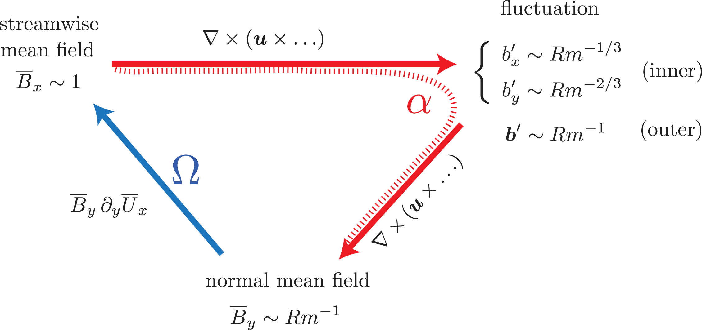
type. The different scalings for the magnitude and localization of the magnetic field variables are also explained. A sketch of the dynamo loop at threshold is given in figure 9 and each of the different steps is discussed in detail.
The optimal dynamo is of
 $\unicode[STIX]{x1D6FC}{-}\unicode[STIX]{x1D6FA}$
type with the particularity that magnetic field fluctuations localize on
 $Rm^{-1/3}$
wide critical layers around
 $y=0,\unicode[STIX]{x03C0}$
, where
 $\overline{\boldsymbol{U}}$
vanishes. This gives rise to inner and outer regions where the scalings for the magnetic fluctuation are different.

4.1 Starting with a dominant streamwise mean magnetic field
 $\overline{B}_{x}\,\boldsymbol{e}_{x}$

The magnetic field driven by the optimal dynamo basically aligns with the mean Kolmogorov flow and has no streamwise dependence. Approximately, this means that
 $$\begin{eqnarray}\overline{\boldsymbol{B}}\approx \overline{B}_{x}(y,z)\,\boldsymbol{e}_{x}.\end{eqnarray}$$
In the following, one may consider
 $\overline{B}_{x}\sim 1$
.
4.2 The interaction
$\unicode[STIX]{x1D735}\times (\boldsymbol{u}\times \overline{\boldsymbol{B}})$
generates a localized magnetic fluctuation
$\boldsymbol{b}^{\prime }$


The mean magnetic field
 $\overline{B}_{x}\boldsymbol{e}_{x}$
is deformed by the optimal perturbation flow that we rewrite as
 $\boldsymbol{u}=Rm^{-1}\boldsymbol{v}$
. Since
 $Rm^{-1}\sim s$
at the optimal dynamo threshold,
 $\boldsymbol{v}$
is an order-one flow. Within the framework of a second-order mean field dynamo model, the magnetic field fluctuation
 $\boldsymbol{b}^{\prime }$
that is driven, needs to satisfy
 $$\begin{eqnarray}\unicode[STIX]{x1D735}\times (\overline{\boldsymbol{U}}\times \boldsymbol{b}^{\prime })+Rm^{-1}\unicode[STIX]{x1D6FB}^{2}\boldsymbol{b}^{\prime }=-Rm^{-1}\unicode[STIX]{x1D735}\times (\boldsymbol{v}\times \overline{\boldsymbol{B}}),\quad \unicode[STIX]{x1D735}\boldsymbol{\cdot }\boldsymbol{b}^{\prime }=0.\end{eqnarray}$$
This set of equations is overdetermined. In practice, we can focus on
 $$\begin{eqnarray}\displaystyle -\text{sin}\,y\unicode[STIX]{x2202}_{x}b_{j}^{\prime }+Rm^{-1}(\unicode[STIX]{x2202}_{xx}^{2}+\unicode[STIX]{x2202}_{yy}^{2}+\unicode[STIX]{x2202}_{zz}^{2})b_{j}^{\prime }=-Rm^{-1}\overline{B}_{x}\unicode[STIX]{x2202}_{x}v_{j} & & \displaystyle\end{eqnarray}$$
and here and further, we use the index
 $j$
to refer to
 $j=y,z$
components. The solenoidality requirement
 $$\begin{eqnarray}\displaystyle \unicode[STIX]{x2202}_{x}b_{x}^{\prime }+\unicode[STIX]{x2202}_{y}b_{y}^{\prime }+\unicode[STIX]{x2202}_{z}b_{z}^{\prime }=0 & & \displaystyle\end{eqnarray}$$
yields
 $b_{x}^{\prime }$
. In the high
 $Rm$
-limit, one can propose an asymptotic solution to this set of equations and a natural guess for the leading-order magnetic fluctuation would be
 $$\begin{eqnarray}b_{y}^{\prime }=Rm^{-1}c_{y}^{\prime }+\cdots\end{eqnarray}$$
with
 $c_{y}^{\prime }$
of order 1. Injected into (4.3a
), the leading balance is at order
 $Rm^{-1}$
and fixes
 $c_{j}^{\prime }$
 $$\begin{eqnarray}-\text{sin}\,y\unicode[STIX]{x2202}_{x}c_{j}^{\prime }=\overline{B}_{x}\unicode[STIX]{x2202}_{x}v_{j}\quad \Rightarrow \quad c_{j}^{\prime }=\frac{\overline{B}_{x}v_{j}}{\sin y}.\end{eqnarray}$$
This diffusionless solution is not correct everywhere in space. In the vicinity of
 $y=0,\unicode[STIX]{x03C0}$
where
 $\overline{\boldsymbol{U}}$
vanishes, it is singular. This means that we must account for a possible sharp variation of the fields in a critical layer spanning the local neighbourhoods of
 $y=0$
and/or
 $y=\unicode[STIX]{x03C0}$
. To model the critical layer, we introduce a zoomed variable
 $\widetilde{y}$
through the relation
 $$\begin{eqnarray}y=\unicode[STIX]{x03C0}+Rm^{-\unicode[STIX]{x1D6FD}}\widetilde{y}\end{eqnarray}$$
for the layer around
 $y=\unicode[STIX]{x03C0}$
. We leave
 $\unicode[STIX]{x1D6FD}>0$
free to determine. Localization of the field structure of
 $\boldsymbol{b}^{\prime }$
means that we need to replace
 $$\begin{eqnarray}\left.\begin{array}{@{}c@{}}b_{y}^{\prime }(y)\rightarrow b_{y}^{\prime }(\,\widetilde{y}\,)\\ b_{z}^{\prime }(y)\rightarrow b_{z}^{\prime }(\,\widetilde{y}\,)\end{array}\right\},\quad \sin y\rightarrow -Rm^{-\unicode[STIX]{x1D6FD}}\widetilde{y}+O(Rm^{-3\unicode[STIX]{x1D6FD}})\end{eqnarray}$$
in this (inner) region. Equation (4.3a ) then reduces to
 $$\begin{eqnarray}Rm^{-\unicode[STIX]{x1D6FD}}\widetilde{y}\unicode[STIX]{x2202}_{x}b_{j}^{\prime }+(Rm^{-1+2\unicode[STIX]{x1D6FD}}\unicode[STIX]{x2202}_{\widetilde{y}\widetilde{y}}+Rm^{-1}(\unicode[STIX]{x2202}_{xx}^{2}+\unicode[STIX]{x2202}_{zz}^{2}))b_{j}^{\prime }=-Rm^{-1}\overline{B}_{x}\unicode[STIX]{x2202}_{x}v_{j}|_{\unicode[STIX]{x03C0}}+O(Rm^{-1-\unicode[STIX]{x1D6FD}}).\end{eqnarray}$$
The notation
 $|_{\unicode[STIX]{x03C0}}$
refers to the field evaluated at
 $y=\unicode[STIX]{x03C0}$
. To find a solution in high
 $Rm$
-limit, one has to admit a different leading-order expansion inside the critical layer
 $$\begin{eqnarray}b_{j}^{\prime }=Rm^{-\unicode[STIX]{x1D6FC}}d_{j}^{\prime }+\cdots\end{eqnarray}$$
with
 $d_{j}^{\prime }$
of order 1 and the exponent
 $0<\unicode[STIX]{x1D6FC}<1$
to be determined. Injecting this expansion in the (4.8), we find that the dominant balance inside the critical layer is
 $$\begin{eqnarray}\displaystyle Rm^{-\unicode[STIX]{x1D6FD}-\unicode[STIX]{x1D6FC}}\widetilde{y}\unicode[STIX]{x2202}_{x}d_{j}^{\prime }+Rm^{-1+2\unicode[STIX]{x1D6FD}-\unicode[STIX]{x1D6FC}}\unicode[STIX]{x2202}_{\widetilde{y}\widetilde{y}}d_{j}^{\prime }=-Rm^{-1}\overline{B}_{x}\unicode[STIX]{x2202}_{x}v_{j}|_{\unicode[STIX]{x03C0}} & & \displaystyle\end{eqnarray}$$
for
 $j=y,z$
. All terms have the same magnitude if
 $$\begin{eqnarray}\left.\begin{array}{@{}c@{}}\unicode[STIX]{x1D6FD}+\unicode[STIX]{x1D6FC}=1\\ 2\unicode[STIX]{x1D6FD}-\unicode[STIX]{x1D6FC}=0\end{array}\right\}\quad \Rightarrow \quad \left.\begin{array}{@{}c@{}}\unicode[STIX]{x1D6FC}=2/3\\ \unicode[STIX]{x1D6FD}=1/3\end{array}\right\}\end{eqnarray}$$
which explains the
 $O(Rm^{-1/3})$
localization of
 $\boldsymbol{b}^{\prime }$
and the scaling laws for the magnitudes of
 $b_{\pm ,y},b_{\pm ,z}$
. The scaling law for the streamwise component
 $b_{\pm ,x}$
can be derived from the solenoidality requirement, that becomes
 $$\begin{eqnarray}\unicode[STIX]{x2202}_{x}b_{x}^{\prime }+Rm^{1/3}\unicode[STIX]{x2202}_{\widetilde{y}}b_{y}^{\prime }+\unicode[STIX]{x2202}_{z}b_{z}^{\prime }=0\end{eqnarray}$$
in the critical layer region. This implies that
 $$\begin{eqnarray}b_{x}^{\prime }=Rm^{-1/3}d_{x}^{\prime }+\cdots\end{eqnarray}$$
with
 $d_{x}^{\prime }$
of order 1, which is the scaling that was suggested for
 $b_{\pm ,x}$
.
In principle, it is possible to pursue the theoretical analysis of the critical layer and to obtain an inner solution formally written in terms of Airy functions. This inner solution needs to be asymptotically matched to the outer solution (4.5) in order to find the magnetic field fluctuation
 $\boldsymbol{b}^{\prime }$
everywhere. This is a rather technical procedure that is not detailed here.
4.3 The interaction
$\unicode[STIX]{x1D735}\times \overline{\boldsymbol{u}\times \boldsymbol{b}^{\prime }}$
generates a small normal mean field
$\overline{B}_{y}\sim Rm^{-1}$


Magnetic field and flow fluctuations interact to regenerate small mean fields
 $\overline{\boldsymbol{B}}$
: this is the essence of the so-called
 $\unicode[STIX]{x1D6FC}$
-effect of dynamo theory. The
 $\unicode[STIX]{x1D6FC}$
-effect can generate all three mean field components weakly, but only the
 $\unicode[STIX]{x1D6FC}$
-regeneration of
 $\overline{B}_{y}$
is crucial in the dynamo mechanism. Denoting
 $\boldsymbol{u}=Rm^{-1}\boldsymbol{v}$
, we find the equation for
 $\overline{B}_{y}$
 $$\begin{eqnarray}\displaystyle Rm^{-1}(\unicode[STIX]{x2202}_{yy}^{2}+\unicode[STIX]{x2202}_{zz}^{2})\overline{B}_{y}=Rm^{-1}\overline{(\boldsymbol{v}\boldsymbol{\cdot }\unicode[STIX]{x1D735})b_{y}^{\prime }}-Rm^{-1}\overline{(\boldsymbol{b}^{\prime }\boldsymbol{\cdot }\unicode[STIX]{x1D735})v_{y}}. & & \displaystyle\end{eqnarray}$$
On the right-hand side of (4.14) we find
 $\boldsymbol{b}^{\prime }$
and since this field is localized near the critical layer, we must consider the balances in the equation, for inner and outer regions separately. Far away from the critical layer, we know that
 $\boldsymbol{b}^{\prime }\sim Rm^{-1}$
. This means that the right-hand side of (4.14) is
 $O(Rm^{-2})$
. A balance with the diffusive terms on the left-hand side is only possible when
 $$\begin{eqnarray}\overline{B}_{y}=Rm^{-1}\overline{C}_{y}+\cdots\end{eqnarray}$$
with
 $\overline{C}_{y}$
an order-one field. This indeed corresponds to the scaling we have found for
 $\overline{B}_{y}$
. In the critical layer region, the balance is different due to the localization. There we have
 $$\begin{eqnarray}(Rm^{2/3}\unicode[STIX]{x2202}_{\widetilde{y}\widetilde{y}}^{2}+O(1))\overline{B}_{y}=Rm^{-1/3}(\overline{v_{y}\unicode[STIX]{x2202}_{\widetilde{y}}d_{y}^{\prime }}-\overline{d_{x}^{\prime }\unicode[STIX]{x2202}_{x}v_{y}}-\overline{d_{y}^{\prime }\unicode[STIX]{x2202}_{\widetilde{y}}v_{y}})+O(Rm^{-2/3}).\end{eqnarray}$$
Equilibrium between both sides requires that
 $$\begin{eqnarray}\overline{B}_{y}=Rm^{-1}\overline{D}_{y}+\cdots\end{eqnarray}$$
in the inner region, with
 $\overline{D}_{y}$
an order-one field. All combined, it seems that the mean magnetic field component
 $\overline{B}_{y}\sim Rm^{-1}$
everywhere. This suggests that the generation of
 $\overline{B}_{y}$
by the
 $\unicode[STIX]{x1D6FC}$
-effect can occur as much inside as outside the critical layer. It also explains why
 $\overline{B}_{y}$
is much less localized than
 $\boldsymbol{b}^{\prime }$
.
For the dynamo process
 $\overline{B}_{z}$
is of no real importance. If desired, one can calculate
 $\overline{B}_{z}$
using the solenoidality of the mean magnetic field,
 $$\begin{eqnarray}\text{(outer)}:\unicode[STIX]{x2202}_{y}\overline{B}_{y}+\unicode[STIX]{x2202}_{z}\overline{B}_{z}=0,\quad \text{(inner)}:Rm^{1/3}\unicode[STIX]{x2202}_{\widetilde{y}}\overline{B}_{y}+\unicode[STIX]{x2202}_{z}\overline{B}_{z}=0.\end{eqnarray}$$
This yields
 $\overline{B}_{z}\sim Rm^{-1}$
in the outer region which is what we observe, but possibly
 $Rm^{-2/3}$
in the critical layer region. This higher value is not really what has been observed although figure 8(a), but also the left panel of figure 8(c) (yellow curves do not align as much near
 $y=\unicode[STIX]{x03C0}$
) indeed suggest that
 $\overline{B}_{z}$
may be slightly bigger than
 $Rm^{-1}$
.
4.4 The transverse
$\overline{B}_{y}\sim Rm^{-1}$
is sheared to regenerate
$\overline{B}_{x}\sim 1$


In the final step, we consider the regeneration of a large streamwise mean field
 $\overline{B}_{x}\sim 1$
out of the small
 $\overline{B}_{y}\sim Rm^{-1}$
due to the background shear. This is the essence of what dynamo theory calls the
 $\unicode[STIX]{x1D6FA}$
-effect. The equation for
 $\overline{B}_{x}$
is
 $$\begin{eqnarray}Rm^{-1}(\unicode[STIX]{x2202}_{yy}^{2}+\unicode[STIX]{x2202}_{zz}^{2})\overline{B}_{x}=-\overline{B}_{y}\cos y-Rm^{-1}(\unicode[STIX]{x1D735}\times \overline{\boldsymbol{v}\times \boldsymbol{b}^{\prime }})_{x}.\end{eqnarray}$$
Far away from critical layer regions, we know that both
 $\boldsymbol{b}^{\prime }$
and
 $\overline{B}_{y}\sim Rm^{-1}$
. This implies that the magnetic stretching term
 $\overline{B}_{y}\cos y$
really is dominant on the right-hand side. With (4.15), the leading-order balance for
 $\overline{B}_{x}$
becomes
 $$\begin{eqnarray}(\unicode[STIX]{x2202}_{yy}^{2}+\unicode[STIX]{x2202}_{zz}^{2})\overline{B}_{x}=-\overline{C}_{y}\cos y,\end{eqnarray}$$
with
 $\overline{C}_{y}$
of order 1. This implies that the large
 $\overline{B}_{x}\sim 1$
that we started with can be regenerated away from the critical layer. In the critical layer region and keeping only the leading-order terms, we find that
 $$\begin{eqnarray}Rm^{-1/3}\unicode[STIX]{x2202}_{\widetilde{y}\widetilde{y}}^{2}\overline{B}_{x}=-Rm^{-1}\overline{D}_{y}+Rm^{-1}(\overline{v_{y}\unicode[STIX]{x2202}_{\widetilde{y}}d_{x}^{\prime }})+O(Rm^{-4/3})\end{eqnarray}$$
that implies
 $$\begin{eqnarray}\unicode[STIX]{x2202}_{\widetilde{y}\widetilde{y}}^{2}\overline{B}_{x}=0.\end{eqnarray}$$
A simple solution to this equation is that
 $\overline{B}_{x}$
is independent of
 $\widetilde{y}$
, which is compatible with what we observe:
 $\overline{B}_{x}$
does not vary by much in the critical layer.
4.5 Summary
In passing through these different steps we have completed one turn in the dynamo feedback loop at threshold. With perturbation flows
 $\boldsymbol{u}$
of magnitude
 $Rm^{-1}$
, it is possible to maintain mean field dynamos with dominant
 $\overline{B}_{x}\sim 1$
it the high-
 $Rm$
limit. Magnetic fluctuations of magnitude
 $b_{y}^{\prime },b_{z}^{\prime }\sim Rm^{-2/3}$
to
 $b_{x}^{\prime }\sim Rm^{-1/3}$
can develop on
 $Rm^{-1/3}$
wide critical layers. The
 $\unicode[STIX]{x1D6FC}$
-effect occurs in this layer but is also active in the bulk and it allows us to regenerate
 $\overline{B}_{y}\sim Rm^{-1}$
. This small normal mean field is amplified and rotated by the shear to regenerate
 $\overline{B}_{x}\sim 1$
, in what we usually call the
 $\unicode[STIX]{x1D6FA}$
-effect in dynamo theory.
5 Conclusion
One-dimensional shear flows such as the Kolmogorov flow are never kinematic dynamos on their own but the addition of small flow perturbations can easily trigger dynamo action. This was suspected more than 50 years ago by the scientists that developed the mean field dynamo theory celebrated in the present special issue. But where mean field dynamo theory provided the mechanisms, it did not allow us to measure what was minimally required on a perturbation flow for it to trigger a dynamo.
In H16 and now also in this article, I have shown that variational optimization algorithms can be used to numerically isolate the smallest possible fluctuation flows that can trigger a dynamo in shear flows. Compared to H16, I replaced the full three-dimensional search space of stationary perturbation flows
 $\boldsymbol{u}$
and magnetic fields
 $\boldsymbol{B}$
with a well-chosen set of modes. This was not a blind guess as it was directly inspired by the outcome of H16. From a practical point of view, this truncation reduces a (costly) three-dimensional optimization problem to a (light) one-dimensional optimization. This allowed us to track the optimal dynamo into the high
 $Rm$
asymptotic regime, inaccessible in H16. From a physical point of view, we optimized the dynamo within the framework of a second-order mean field dynamo model.
The outcome of this study is very satisfying. First of all, we have confirmed the scaling law
 $s_{\text{min}}\sim Rm^{-1}$
for the minimal magnitude of dynamo triggering perturbation flows. As a simple reinterpretation of this scaling law, we now propose that a dynamo requires perturbation magnetic Reynolds numbers
 $Rm_{s}=s_{\ast }{L_{\ast }}^{2}/4\unicode[STIX]{x03C0}^{2}\unicode[STIX]{x1D702}_{\ast }$
in the high
 $Rm$
-limit. Physically, this tells us that the true magnitude
 $U_{\ast }$
of the dominant mean flow is not important for the onset of dynamo at high
 $Rm=U_{\ast }L_{\ast }/4\unicode[STIX]{x03C0}\unicode[STIX]{x1D702}_{\ast }$
.
As we could reach into the high
 $Rm$
-regime, we were also able to identify that the optimal perturbation flow rescaled by
 $s$
(or
 $Rm^{-1}$
) has a spatial structure that is almost independent of
 $Rm$
. This is a compelling feature that still needs to be explained. We were able to propose a simplified structure for the optimal perturbation flow.
The magnetic field driven by the optimal dynamo also shows signs of an underlying high
 $Rm$
-asymptotic structure. We were able to identify a simplified expression for the magnetic eigenmode. Analysis of the dynamo mechanism suggest that the high
 $Rm$
optimal dynamo is a mean field dynamo of
 $\unicode[STIX]{x1D6FC}{-}\unicode[STIX]{x1D6FA}$
type, with a particularity that at least part of the
 $\unicode[STIX]{x1D6FC}$
-effect occurs on a critical layer. Similar high
 $Rm$
-mean field dynamos with critical layers appear in the context of the Braginsky dynamo (Braginsky & Roberts Reference Braginsky and Roberts1975). It is possible that our optimal dynamos may be correctly modelled using that particular high-
 $Rm$
approach to mean field dynamo action.
The dynamo problem that we have studied here is very similar to the hydrodynamical problem of subcritical transition to turbulence. Shear flows such as Couette flow or pipe flow are linearly stable for all values of the Reynolds number
 $Re$
, but they do become turbulent in experiments beyond some value of
 $Re$
. The transition is triggered by finite amplitude flow perturbations and it has also been of interest to measure their minimal magnitude as a function of
 $Re$
. Several scaling laws have been proposed from theoretical, numerical or experimental studies and the particular law
 $u_{\text{min}}\sim Re^{-1}$
similar to what we found, also appears in Waleffe (Reference Waleffe1997), Chapman (Reference Chapman2002), Hof, Juel & Mullin (Reference Hof, Juel and Mullin2003), Ben-Dov & Cohen (Reference Ben-Dov and Cohen2007), Mellibovsky & Meseguer (Reference Mellibovsky and Meseguer2007), Peixinho & Mullin (Reference Peixinho and Mullin2007), Duguet, Brandt & Larsson (Reference Duguet, Brandt and Larsson2010), Cherubini, Palma & Robinet (Reference Cherubini, Palma and Robinet2015). Apart from that, one can notice that the
 $\unicode[STIX]{x1D6FC}{-}\unicode[STIX]{x1D6FA}$
diagram of figure 9 is very similar to those diagrams that are used to explain the self-sustaining process (SSP) (Waleffe Reference Waleffe1997). If in figure 9,
 $\boldsymbol{B}$
were to be a flow instead of a magnetic field, then
 $\overline{B}_{x}$
would be a strong streamwise mean flow perturbation often called a ‘streak’ in subcritical transition literature. The smaller normal field
 $\overline{B}_{y},\overline{B}_{z}$
would carry the name ‘roll’ and
 $\boldsymbol{u}$
and
 $\boldsymbol{b}^{\prime }$
would be the ‘wavy disturbances’ that ‘nonlinearly regenerate’
 $\overline{B}_{y}$
. Critical layers similar to the ones observed in the present study also occur in the high
 $Re$
-limit descriptions of self-sustaining states (Wang, Gibson & Waleffe Reference Wang, Gibson and Waleffe2007; Hall & Sherwin Reference Hall and Sherwin2010; Deguchi & Hall Reference Deguchi and Hall2015). Finally, we can suggest Biau & Bottaro (Reference Biau and Bottaro2009), Pralits, Bottaro & Cherubini (Reference Pralits, Bottaro and Cherubini2015) to any mean field dynamo scientist. These fairly recent articles are true hydrodynamical analogues of our
 $\unicode[STIX]{x1D6FC}{-}\unicode[STIX]{x1D6FA}$
mean field dynamos. The hydrodynamical study of (Pralits et al.
Reference Pralits, Bottaro and Cherubini2015) is particularly close to what we did in this article.
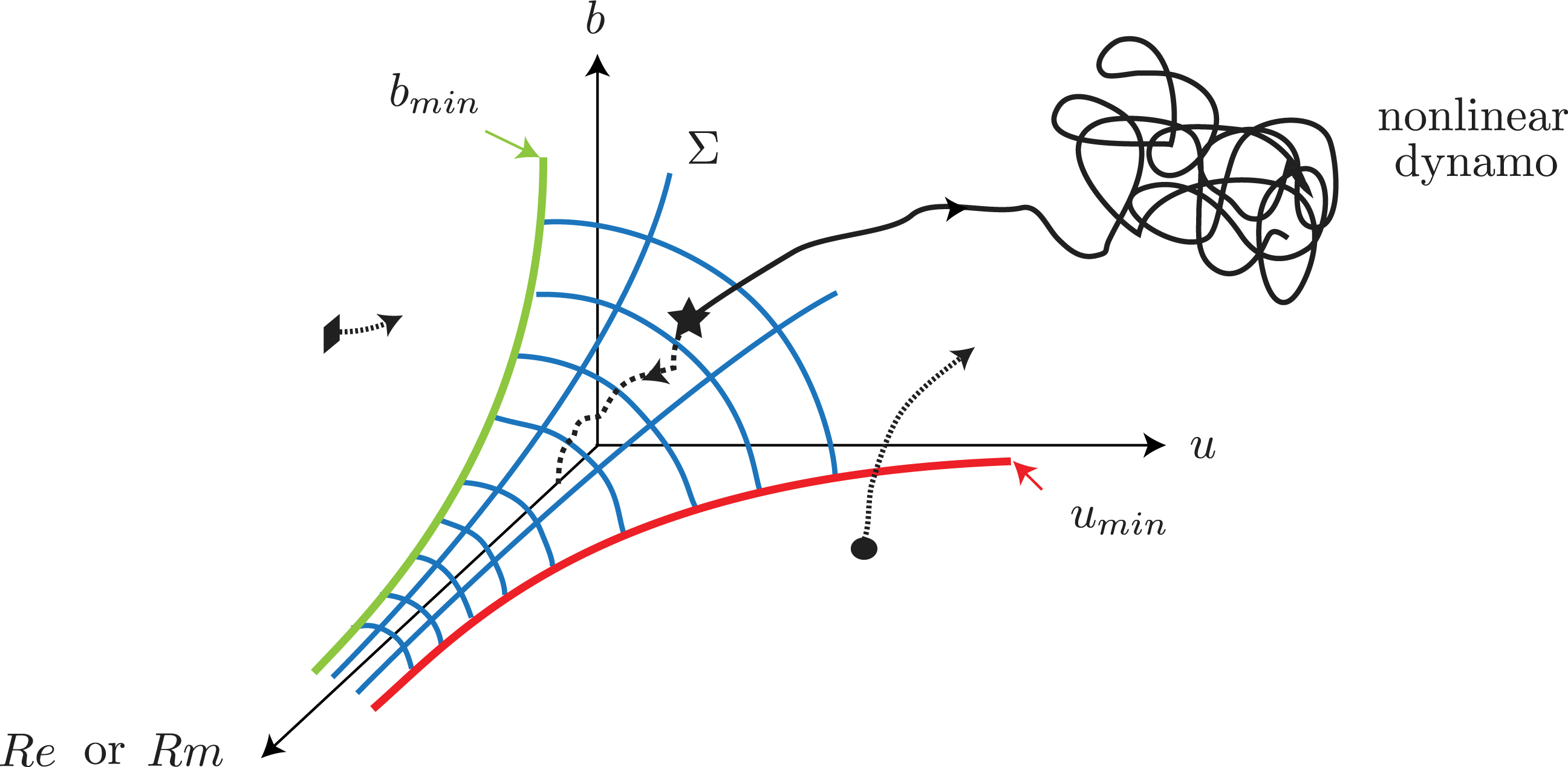
Phase space representation of the magnetohydrodynamical boundary
 $\unicode[STIX]{x1D6F4}$
that separates the laminar shear flow state
 $u=b=0$
, from the nonlinear dynamo state. Pure flow perturbations with magnitudes
 $u>u_{\text{min}}$
(●) or pure magnetic field perturbations with magnitudes
 $b>b_{\text{min}}$
(▪) can trigger transition to a nonlinear dynamo, but in general we expect that a combination of both
 $u$
and
 $b$
also triggers the transition. Slightly above or under a state (
 $\star$
) on the boundary
 $\unicode[STIX]{x1D6F4}$
, perturbations
 $u$
and
 $b$
can either grow out towards a nonlinear dynamo state (black full line) or relaminarize back to
 $u,b=0$
(black dotted line). We expect this nozzle shape of the surface
 $\unicode[STIX]{x1D6F4}$
, since minimal magnitudes of dynamo triggering perturbations
 $u$
and
 $b$
likely decrease with increasing Reynolds or magnetic Reynolds numbers
 $Re$
or
 $Rm$
.

Considering the 50 year heritage of mean field dynamo theory, it is possible that some of our mean field dynamo tools transpose to the subcritical transition problem. Conversely, with so many flows that can alone not be dynamos, there is an immense potential in dynamo theory for the variational optimization methods that are now being deployed in the subcritical transition problem. Nonlinear dynamos that are self-sustaining in ways similar to the SSP of Waleffe (Reference Waleffe1997) have been proposed by Rincon, Ogilvie & Proctor (Reference Rincon, Ogilvie and Proctor2007), Rincon et al. (Reference Rincon, Ogilvie, Proctor and Cossu2008) and they were found by Herault et al. (Reference Herault, Rincon, Cossu, Lesur, Ogilvie and Longaretti2011), Riols et al. (Reference Riols, Rincon, Cossu, Lesur, Longaretti, Ogilvie and Herault2013, Reference Riols, Rincon, Cossu, Lesur, Ogilvie and Longaretti2015) in shearing boxes and more recently in quasi-Keplerian Taylor–Couette flows (Guseva et al.
Reference Guseva, Hollerbach, Willis and Avila2017). This implies that subcritical nonlinear dynamo branches exist in shear flows and we now need to map out how much flow or magnetic field perturbation is necessary to trigger transition to such nonlinear dynamo states. Figure 10 gives a phase space impression of how the ‘laminar flow’–‘nonlinear dynamo’ boundary may look for nonlinear dynamos in shear flows. With a variational method that can optimize magnetic field growth in the full magneto hydro dynamical (MHD) problem, it should be possible to locate the position of the edge of dynamo
 $\unicode[STIX]{x1D6F4}$
in this diagram. I hope to report on this topic in the future.
Acknowledgement
The author thanks Y. Duguet for interesting discussions on the problem of subcritical transition to turbulence.
Appendix A. Supplementary information on optimization loop
The Lagrangian functional (2.7) needs to be modified in order to take into account the truncation of the flow, the magnetic field and the mean field equations (2.12). With many more explicit variables, this looks awkward
 $$\begin{eqnarray}\displaystyle {\mathcal{L}} & = & \displaystyle \ln (2\langle |\overline{\boldsymbol{b}}(y,T)|^{2}\rangle +2\langle |\boldsymbol{b}_{+}(y,T)|^{2}\rangle +2\langle |\boldsymbol{b}_{-}(y,T)|^{2}\rangle )\nonumber\\ \displaystyle & & \displaystyle -\,\langle \overline{p}\unicode[STIX]{x1D735}_{\!0,0}\boldsymbol{\cdot }\overline{\boldsymbol{u}}\rangle +\langle p\unicode[STIX]{x1D735}_{\!1,0}\boldsymbol{\cdot }\boldsymbol{w}\rangle +\langle p_{+}\unicode[STIX]{x1D735}_{\!1,2}\boldsymbol{\cdot }\boldsymbol{w}_{+}\rangle +\langle p_{-}\unicode[STIX]{x1D735}_{\!1,-2}\boldsymbol{\cdot }\boldsymbol{w}_{-}\rangle \nonumber\\ \displaystyle & & \displaystyle -\,\unicode[STIX]{x1D706}_{1}(\langle (\unicode[STIX]{x1D735}_{\!0,0}\times \overline{\boldsymbol{u}})^{2}\rangle +2\langle (\unicode[STIX]{x1D735}_{\!1,0}\times \boldsymbol{w})^{2}\rangle +2\langle (\unicode[STIX]{x1D735}_{\!1,2}\times \boldsymbol{w}_{+})^{2}\rangle +2\langle (\unicode[STIX]{x1D735}_{\!1,-2}\times \boldsymbol{w}_{-})^{2}\rangle -s^{2})\nonumber\\ \displaystyle & & \displaystyle -\,\langle \overline{q}\unicode[STIX]{x1D735}_{\!0,1}\boldsymbol{\cdot }\overline{\boldsymbol{b}}\rangle +\langle q_{+}\unicode[STIX]{x1D735}_{\!1,1}\boldsymbol{\cdot }\boldsymbol{b}_{+}\rangle +\langle q_{-}\unicode[STIX]{x1D735}_{\!1,-1}\boldsymbol{\cdot }\boldsymbol{b}_{-}\rangle \nonumber\\ \displaystyle & & \displaystyle -\,\unicode[STIX]{x1D706}_{2}(2\langle |\overline{\boldsymbol{b}}(y,0)|^{2}\rangle +2\langle |\boldsymbol{b}_{+}(y,0)|^{2}\rangle +2\langle |\boldsymbol{b}_{-}(y,0)|^{2}\rangle -1)\nonumber\\ \displaystyle & & \displaystyle -\,\int _{0}^{T}\langle \overline{\boldsymbol{b}}^{\dagger }\boldsymbol{\cdot }(\unicode[STIX]{x2202}_{t}\overline{\boldsymbol{b}}-\cdots )+\boldsymbol{b}_{+}^{\dagger }\boldsymbol{\cdot }(\unicode[STIX]{x2202}_{t}\boldsymbol{b}_{+}-\cdots )+\boldsymbol{b}_{-}^{\dagger }\boldsymbol{\cdot }(\unicode[STIX]{x2202}_{t}\boldsymbol{b}_{-}\ldots )\rangle \,\text{d}t.\end{eqnarray}$$
In the last line, we abbreviated the notation by suggesting (2.12) of the mean field model. We introduced the fields
 $\bar{p},p,p_{\pm }$
and
 $\bar{q},q_{\pm }$
to express the solenoidality constraints. Adjoint magnetic fields are truncated as in (2.10) and denoted by the variables
 $\overline{\boldsymbol{b}}^{\dagger },\boldsymbol{b}_{\pm }^{\dagger }$
. The non-trivial Euler–Lagrange equations are found by partial integration. The equations
 $\unicode[STIX]{x1D6FF}{\mathcal{L}}/\unicode[STIX]{x1D6FF}\overline{\boldsymbol{b}}=0$
,
 $\unicode[STIX]{x1D6FF}{\mathcal{L}}/\unicode[STIX]{x1D6FF}\boldsymbol{b}_{\pm }=0$
define the adjoint system of (2.12):
 $$\begin{eqnarray}\displaystyle -\unicode[STIX]{x2202}_{t}\overline{\boldsymbol{b}}^{\dagger } & = & \displaystyle (\unicode[STIX]{x1D735}_{\!0,1}\times \overline{\boldsymbol{b}}^{\dagger })\times (\overline{\boldsymbol{U}}+\overline{\boldsymbol{w}})\nonumber\\ \displaystyle & & \displaystyle +\,(\unicode[STIX]{x1D735}_{\!1,-1}\times \boldsymbol{b}_{-}^{\dagger })^{\ast }\times \boldsymbol{w}+(\unicode[STIX]{x1D735}_{\!1,1}\times \boldsymbol{b}_{+}^{\dagger })\times \boldsymbol{w}^{\ast }\nonumber\\ \displaystyle & & \displaystyle +\,(\unicode[STIX]{x1D735}_{\!1,1}\times \boldsymbol{b}_{+}^{\dagger })^{\ast }\times \boldsymbol{w}_{+}+(\unicode[STIX]{x1D735}_{\!1,-1}\times \boldsymbol{b}_{-}^{\dagger })\times \boldsymbol{w}_{-}^{\ast }+Rm^{-1}\unicode[STIX]{x1D6FB}_{0,1}^{2}\overline{\boldsymbol{b}}^{\dagger }\end{eqnarray}$$
 $$\begin{eqnarray}\displaystyle -\unicode[STIX]{x2202}_{t}\boldsymbol{b}_{+}^{\dagger } & = & \displaystyle (\unicode[STIX]{x1D735}_{\!1,1}\times \boldsymbol{b}_{+}^{\dagger })\times (\overline{\boldsymbol{U}}+\overline{\boldsymbol{w}})\nonumber\\ \displaystyle & & \displaystyle +\,(\unicode[STIX]{x1D735}_{\!0,1}\times \overline{\boldsymbol{b}}^{\dagger })\times \boldsymbol{w}+(\unicode[STIX]{x1D735}_{\!0,1}\times \overline{\boldsymbol{b}}^{\dagger })^{\ast }\times \boldsymbol{w}_{+}+Rm^{-1}\unicode[STIX]{x1D6FB}_{1,1}^{2}\boldsymbol{b}_{+}^{\dagger }\end{eqnarray}$$
 $$\begin{eqnarray}\displaystyle -\unicode[STIX]{x2202}_{t}\boldsymbol{b}_{-}^{\dagger } & = & \displaystyle (\unicode[STIX]{x1D735}_{\!1,-1}\times \boldsymbol{b}_{-}^{\dagger })\times (\overline{\boldsymbol{U}}+\overline{\boldsymbol{w}})\nonumber\\ \displaystyle & & \displaystyle +\,(\unicode[STIX]{x1D735}_{\!0,1}\times \overline{\boldsymbol{b}}^{\dagger })^{\ast }\times \boldsymbol{w}+(\unicode[STIX]{x1D735}_{\!0,1}\times \overline{\boldsymbol{b}}^{\dagger })\times \boldsymbol{w}_{-}+Rm^{-1}\unicode[STIX]{x1D6FB}_{1,-1}^{2}\boldsymbol{b}_{-}^{\dagger }.\end{eqnarray}$$
The variational derivatives needed to update the flow variables are
 $$\begin{eqnarray}\displaystyle \frac{\unicode[STIX]{x1D6FF}{\mathcal{L}}}{\unicode[STIX]{x1D6FF}\overline{\boldsymbol{w}}} & = & \displaystyle 2Re\int _{0}^{T}[\overline{\boldsymbol{b}}^{\ast }\times (\unicode[STIX]{x1D735}_{\!0,1}\times \overline{\boldsymbol{b}}^{\dagger })+\boldsymbol{b}_{+}^{\ast }\times (\unicode[STIX]{x1D735}_{\!1,1}\times \boldsymbol{b}_{+}^{\dagger })+\boldsymbol{b}_{-}^{\ast }\times (\unicode[STIX]{x1D735}_{\!1,1}\times \boldsymbol{b}_{-}^{\dagger })]\,\text{d}t\nonumber\\ \displaystyle & & \displaystyle +\,2\unicode[STIX]{x1D706}_{2}\unicode[STIX]{x1D6FB}_{0,0}^{2}\overline{\boldsymbol{w}}+\unicode[STIX]{x1D735}_{\!0,0}\overline{p}\end{eqnarray}$$
 $$\begin{eqnarray}\displaystyle \frac{\unicode[STIX]{x1D6FF}{\mathcal{L}}}{\unicode[STIX]{x1D6FF}\boldsymbol{w}} & = & \displaystyle \!\int _{0}^{T}\![\boldsymbol{b}_{-}\times (\unicode[STIX]{x1D735}_{\!0,1\!}\times \overline{\boldsymbol{b}}^{\dagger })+\boldsymbol{b}_{+}\times (\unicode[STIX]{x1D735}_{\!0,1\!}\times \overline{\boldsymbol{b}}^{\dagger })^{\ast }+\overline{\boldsymbol{b}}^{\ast }\times (\unicode[STIX]{x1D735}_{\!1,1\!}\times \boldsymbol{b}_{+}^{\dagger })+\overline{\boldsymbol{b}}\times (\unicode[STIX]{x1D735}_{\!1,-1\!}\times \boldsymbol{b}_{-}^{\dagger })]\,\text{d}t\nonumber\\ \displaystyle & & \displaystyle +\,2\unicode[STIX]{x1D706}_{2}\unicode[STIX]{x1D6FB}_{1,0}^{2}\boldsymbol{w}+\unicode[STIX]{x1D735}_{\!1,0}p\end{eqnarray}$$
 $$\begin{eqnarray}\displaystyle & \displaystyle \frac{\unicode[STIX]{x1D6FF}{\mathcal{L}}}{\unicode[STIX]{x1D6FF}\boldsymbol{w}_{+}}=\!\int _{0}^{T}\![\boldsymbol{b}_{+}\times (\unicode[STIX]{x1D735}_{\!0,1}\times \overline{\boldsymbol{b}}^{\dagger })+\overline{\boldsymbol{b}}\times (\unicode[STIX]{x1D735}_{\!1,1}\times \boldsymbol{b}_{+}^{\dagger })]\,\text{d}t+2\unicode[STIX]{x1D706}_{2}\unicode[STIX]{x1D6FB}_{1,2}^{2}\boldsymbol{w}_{+}+\unicode[STIX]{x1D735}_{\!1,2}p_{+}\quad & \displaystyle\end{eqnarray}$$
 $$\begin{eqnarray}\displaystyle & \displaystyle \frac{\unicode[STIX]{x1D6FF}{\mathcal{L}}}{\unicode[STIX]{x1D6FF}\boldsymbol{w}_{-}}=\!\int _{0}^{T}\![\boldsymbol{b}_{-}\times (\unicode[STIX]{x1D735}_{\!0,1}\times \overline{\boldsymbol{b}}^{\dagger })^{\ast }+\overline{\boldsymbol{b}}^{\ast }\times (\unicode[STIX]{x1D735}_{\!1,-1}\times \boldsymbol{b}_{-}^{\dagger })]\,\text{d}t+2\unicode[STIX]{x1D706}_{2}\unicode[STIX]{x1D6FB}_{1,-2}^{2}\boldsymbol{w}_{-}+\unicode[STIX]{x1D735}_{\!1,-2}p_{-}.\quad & \displaystyle\end{eqnarray}$$
The variational derivatives needed to update the initial magnetic field are
 $$\begin{eqnarray}\frac{\unicode[STIX]{x1D6FF}{\mathcal{L}}}{\unicode[STIX]{x1D6FF}\overline{\boldsymbol{b}}_{0}}=\overline{\boldsymbol{b}}_{0}^{\dagger }-2\unicode[STIX]{x1D706}_{2}\overline{\boldsymbol{b}}_{0}+\unicode[STIX]{x1D735}_{\!0,1}\overline{q},\quad \frac{\unicode[STIX]{x1D6FF}{\mathcal{L}}}{\unicode[STIX]{x1D6FF}\overline{\boldsymbol{b}}_{\pm ,0}}=\boldsymbol{b}_{\pm ,0}^{\dagger }-2\unicode[STIX]{x1D706}_{2}\boldsymbol{b}_{\pm ,0}+\unicode[STIX]{x1D735}_{\!1,\pm 1}q_{\pm }.\end{eqnarray}$$
In the numerical implementation of the optimization algorithm, we expand all fields in Fourier series along
 $y$
, e.g.
 $$\begin{eqnarray}\overline{\boldsymbol{b}}(y,t)=\mathop{\sum }_{k=-N/2+1}^{N/2}\hat{\overline{\boldsymbol{b}}}(k,t)\text{e}^{\text{i}ky}.\end{eqnarray}$$
The optimization loop itself follows the same path as in Willis (Reference Willis2012), Chen et al. (Reference Chen, Herreman and Jackson2015), Herreman (Reference Herreman2016). The direct and adjoint mean field equations are integrated forward and backward in time using a standard
 $2/3$
dealiased pseudospectral solver (exact integration rule for diffusion, second-order predictor–corrector for product terms). Time integrals in
 $\unicode[STIX]{x1D6FF}{\mathcal{L}}/\unicode[STIX]{x1D6FF}\overline{\boldsymbol{w}}$
,
 $\unicode[STIX]{x1D6FF}{\mathcal{L}}/\unicode[STIX]{x1D6FF}\boldsymbol{w}$
and
 $\unicode[STIX]{x1D6FF}{\mathcal{L}}/\unicode[STIX]{x1D6FF}\boldsymbol{w}_{\pm }$
are calculated using Simpson’s rule. The flow variables and the initial magnetic fields are updated using the same scheme as in Chen et al. (Reference Chen, Herreman and Jackson2015).