II. THE NEED FOR ACCURATE ABSORPTION COEFFICIENTS

In some cases absorption coefficients could be completely ignored: an example is analyzing always the same trace elements in the same amount of liquid always disposed in the same vessel: it is often easy to prepare a few standards using the pure liquid and weighted amounts of the analytes and assume a linear relationship between the measured intensity and the concentration. This method automatically corrects for all absorption effects and is actually the most accurate when it can be used.

At the other end of the procedures range, if the excitation device, the geometry of the experiment (solid angles etc.) and the detector can be quantitatively characterized to a reasonable accuracy, a fully standard-less theoretical measurement can be performed (Beckhoff, Reference Beckhoff2008).

In real life, the above two procedures can seldom be used, and the most common implementation of an XRF concentration measurement is to empirically calibrate as a whole the excitation flux and the spectrometer sensitivity function on the one hand, and use a model of the measured sample on the other hand. The sample model can be empirical or based on FP, the spectrometer sensitivity function can encompass detector quantum efficiency or not, etc. Nonetheless, whatever the method, there is an underlying sample model; even in the simplest empirical case the implicit model is “the unknown sample is sufficiently similar to the standards”

Modeling of the sample by using databases of parameters has traditionally been referred to as the fundamental parameters approach, those fundamental parameters include:

• • Electronic shell properties

• • Transitions

• • Mass absorption coefficients

The emission of a homogeneous sample excited by a parallel beam and measured at a fixed angle has been derived almost 60 years ago by Sherman (Reference Sherman1955) and extended to various cases by several authors.

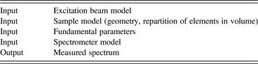
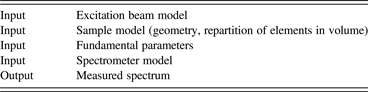
We assume that after little or huge intellectual effort the model is eventually represented by a set of mathematical equations that bind together the aforementioned XRF model components (Table I).

Table I.

Components of the XRF model.

III. WHAT IS CALIBRATION?

Calibration is the process in which concentrations of the samples are known and the unknown parameters of the model are fitted, usually to minimize in the least square sense the differences between computed and known values of concentrations of the standards.

By contrast, routine measurement is the process in which concentrations (and/or geometrical properties) of the samples are to be determined while the other parameters are known and are held fixed.

Whatever the model used, the key to a working evaluation is that the very same math is used for calibration and for evaluation of unknown samples.

In the model equations we alluded to before, the FP do not stand at a particular place from a mathematical point of view, so if it is possible to refine the instrument parameters from measurements of standards it is also possible to refine atomic data, so are the fundamental parameters really fundamental or are any fitted data suitable?

Sherman's model can be written as

$$I\, _{{\rm element}\comma \, {\rm sample}} /I_{{\rm pure}\, {\rm element}} = f \left({{\rm sample}} \right)\ast C_{{\rm element\comma }\, {\rm sample}}$$

where f (sample) is a function of sample composition, thus it depends on C _{element, sample} among others and the linearity is indeed only apparent. Any model that ties a single element concentration to a single line intensity can be written this way after changing variables if needed, and f(sample) can be referred to as an absorption correction function with the obvious property that f(pure element) ≡ 1.0

In Sherman's derivation of f (sample) and as long as higher order fluorescence is neglected, the absorption coefficients appear homogeneously at the numerator and at the denominator of a fraction, and there is the illusion that the MAC need only be known relatively to each other. This illusion is further entertained by the calibration technique: in some sense the errors committed at the calibration step are undone at the evaluation step. However, the illusion quickly vanishes in many practical cases; three examples follow:

• • When secondary emission is taken into account, the emission properties of the intervening transitions have to be taken into account, those parameters could be fitted too, but fixing both the absorption and the emission starts to be a real challenge, probably more complicated than using the real values.

• • Analyzing impurities in light matrices like RoHS: it is simply impractical to have standards matching size and light element concentrations of every sample that can be analyzed.

• • More generally, whenever the physical dimensions of the sample matter, those dimensions use real length and mass units and the absorption must be known in real units as well to guarantee homogeneity of equations.

The second example also shows that we do not only need accurate data but also uncertainty data: when regulatory issues are at stake results should certainly be given with limits of confidence. While the uncertainty is fairly easy to calculate at most of the steps in the process, the exactness of the absorption tables is simply not known.

In this situation, our naïve approach has been to compare the existing datasets. This is indeed naïve because the original sources of many data may be same; furthermore the used criterion relies on the average of several sources and therefore favors data coming from a common source, whereas there is no guarantee that the less used alternate source is not the only good one. Two historic databases are listed in the references because they looked important to us but have not directly been used because we were not aware of machine readable media containing them: the works by Cauchois et al. (Reference Cauchois and Senemaud1978) and by Mac Master et al. (Reference McMaster, Del Grande, Mallett and Hubbell1969). Therefore our approach only tries to single out the discrepancies and leaves open the question of which database is the best one.

IV. A HOME BREWED COMPARISON TOOL

There probably are off-the-shelf comparison programs that could be used, but finding one and adapting it to our goal was probably no simpler than writing a small dedicated tool. The graphical presentation (X-axis = square root of energy, Y-axis = atomic number, coloring = relative discrepancy) had formerly been used by De Boer. The code looks for all DLLs in the same directory as the executable having at least two procedures called respectively “Absorption” and “Author”, and assumes that they can be used to return the mass absorption of an element at a given energy on the one hand and the name of the author of the compilation on the other hand; it loads the relevant DLLs and produces a comparison chart.

For any selected database i (1 ≤ i ≤ N), at energy E, atomic number Z, let the mass absorption coefficient

$$\mu \left({E\comma \; \, Z\comma \; \, i} \right)=A_i\semicolon \; \quad 0. 1 \leq E \leq 60{\rm keV}\semicolon \; \quad 1 \leq Z \leq 94$$

the deviation of interest is D(E, Z) = (max_/i |A _i–A*|)/A*, where A* = (∑A _i)/N.

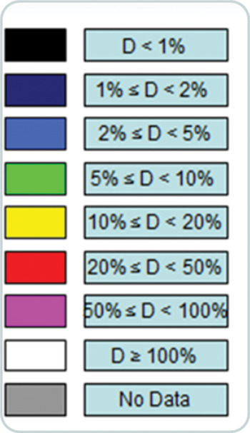
The color code for the graphics is displayed on the next page (see Figure 1).

• • For 200 values of energy selected on a square root scale, the deviation is presented as a colored rectangle in the Z, E plane.

• • The right click menu at any selected location makes it possible to display a zoom on the absorption curves, to help figure out the reason for a discrepancy at a specific location in the display plane.

Figure 1.

Color code for the graphics.

Some case studies follow to illustrate the use of the comparison tool:

• • Comparison of the six databases shows the general trend

• • Zooming in on the low energy region shows the issues, mostly below 1000 eV

• • Comparison of the three most recent tables mostly shows discrepancies on the edge positions

• • Comparison with De Boer's work shows interesting differences in jump ratios.

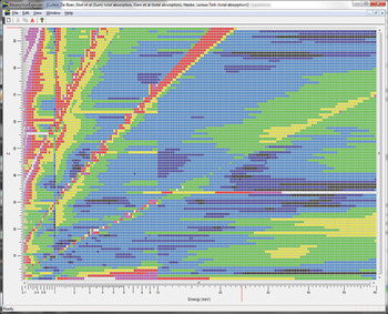
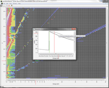
There are striking features in the global comparison sheet (Leroux and Thinh, Reference Leroux and Thinh1977; Plechaty et al., Reference Plechaty, Cullen and Howerton1981; Henke et al., Reference Henke, Lee, Tanaka, Shimabukuro and Fujikawa1982; De Boer, Reference De Boer1988; Elam et al., Reference Elam, Ravel and Sieber2001; Ebel et al., Reference Ebel, Svagera, Ebel, Shaltout and Hubbell2003) (see Figure 2):

• • The 1000 eV vertical separation is clearly visible, simply showing that no reliable data exist below 1000 eV; the 10 keV separation is an artifact caused by one of our databases (Henke et al., Reference Henke, Lee, Tanaka, Shimabukuro and Fujikawa1982) restricted to 10 keV.

• • Many discrepancies occur along the K, L, and M edges (the edges are roughly aligned on inclined lines because of the use of a square root of energy X-axis).

• • Dubious near exact agreement for some elements, some of them exotic (e.g. Z = 85, At) showing that a single source of data – probably quite old – has been used by all authors.

• • Poor agreement for H and He at all energies, whereas Li is in better agreement.

Figure 2.

Global comparison sheet (Leroux and Thinh, Reference Leroux and Thinh1977; Cullen, 1981; Henke et al., Reference Henke, Lee, Tanaka, Shimabukuro and Fujikawa1982; De Boer, Reference De Boer1988; Elam et al., Reference Elam, Ravel and Sieber2001; Ebel et al., Reference Ebel, Svagera, Ebel, Shaltout and Hubbell2003).

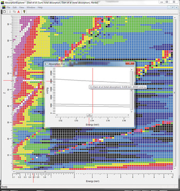
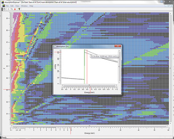
The low energy region zoomed. Elam et al. (Reference Elam, Ravel and Sieber2001) and Ebel et al. (Reference Ebel, Svagera, Ebel, Shaltout and Hubbell2003) are in good agreement in the high-energy region, so it was tempting to compare them in the low-energy region although Ebel explicitly states that the data below 1000 eV should not be regarded as valid (See Figure 3). Henke's table (Reference Henke, Lee, Tanaka, Shimabukuro and Fujikawa1982) was also selected because this work is the first one to address the region below 1000 eV for which we had complete machine readable data.

Figure 3.

Low-energy region zoomed (Henke et al., Reference Henke, Lee, Tanaka, Shimabukuro and Fujikawa1982; Elam et al., Reference Elam, Ravel and Sieber2001; Ebel et al., Reference Ebel, Svagera, Ebel, Shaltout and Hubbell2003).

The region from 100 to 1000 eV also markedly shows the L and M discontinuities, this is even more marked because Henke's table does not supply continuous data, so the code merely interpolates across the edges, causing more artificial discrepancies.

In addition, there are a few horizontal lines showing complete disagreement between Elam's and the other two tables (Z = 55, Cs Elam's data ca. 4 times higher; Z = 60, Nd)

There is overall good agreement, with the already noted exception of edge vicinity, and a rare case of interpolation error in Elam's table, where the first derivative is low and the second derivative high where the contrary would be expected (a typo?) (See Figure 4).

Figure 4.

The three most recent tables (Cullen, 1981; Elam et al., Reference Elam, Ravel and Sieber2001; Ebel et al., Reference Ebel, Svagera, Ebel, Shaltout and Hubbell2003) compared.

Comparing Elam et al. (Reference Elam, Ravel and Sieber2001), Ebel et al. (Reference Ebel, Svagera, Ebel, Shaltout and Hubbell2003), and De Boer (Reference De Boer1988) (see Figure 5), the table shows many jump factors that are significantly higher than the ones found in other authors’ work, this may indicate that De Boer has had access to other sources; it might be interesting to retrieve more original data sources.

Figure 5.

Comparing Elam et al. (Reference Elam, Ravel and Sieber2001), Ebel et al. (Reference Ebel, Svagera, Ebel, Shaltout and Hubbell2003), and De Boer (Reference De Boer1988).