2. Preliminaries

This preliminary section offers a brief review of a number of well-known distributions and stochastic processes: tempered stable distributions, inverse Gaussian distributions, TS subordinators, non-Gaussian Ornstein–Uhlenbeck processes, and two important types of non-Gaussian Ornstein–Uhlenbeck process. They provide the foundations for developing simulation algorithms later in the next section.

2.1. Tempered stable distribution and tempered stable subordinator

Positive tempered stable distribution can be obtained from a one-sided $\alpha$ -stable law by exponential tilting [Reference Barndorff-Nielsen, Nicolato and Shephard11, page 14]; see also [Reference Barndorff-Nielsen and Shephard6, page 3]. More precisely, it can be defined as follows.

Definition 2.1. (Positive tempered stable distribution.) Positive tempered stable (TS) distribution, denoted by $\mathsf{TS}(\alpha,\beta,\theta)$ , is an infinitely divisible distribution defined by its Lévy measure

(2.1) \begin{equation}\nu({\text{d}} y)=\dfrac{\theta}{y^{\alpha+1}}\,{\text{e}}^{-\beta y}\,{\text{d}} y, \quad y\geq 0, \quad \alpha\in(0,1), \quad \beta, \theta \in \mathbb{R}^+,\end{equation}

where $\alpha$ is the stability index, $\theta$ is the intensity parameter, and $\beta$ is the tilting parameter.

In particular, if $\alpha=\frac{1}{2}$ , it reduces to a very important distribution, the inverse Gaussian (IG) distribution (which can be interpreted as the distribution of the first passage time of a Brownian motion to an absorbing barrier).

A tempered stable subordinator is a positive Lévy process whose one-dimensional distributions are positive TS distributions. More precisely, it can be defined as follows.

Definition 2.2. (Tempered stable subordinator.) A tempered stable (TS) subordinator is a positive Lévy process $\{Z_t\,\colon\, t\ge 0 \}$ such that $Z_1$ follows a positive TS distribution, i.e. $Z_1 \sim \mathsf{TS}(\alpha,\beta,\theta)$ .

It is a Lévy subordinator, i.e. a Lévy process with non-decreasing paths (see [Reference Bertoin12, Chapter 3] and [Reference Sato48]), where the state space is restricted in the positive half real line, and $Z_t \sim \mathsf{TS}(\alpha, \beta,\theta t)$ , for all $t>0$ . The stable index $\alpha$ determines the importance of small jumps for the process trajectories, the intensity parameter $\theta$ controls the intensity of jumps, and the tilting parameter $\beta$ determines the decay rate of large jumps. The TS subordinator (including the IG subordinator as a special case) is one of the most general and widely used building blocks for constructing many useful TS-based stochastic processes. Distinguished examples include the TS-based non-Gaussian OU processes, which are briefly reviewed as follows.

2.2. Non-Gaussian Ornstein–Uhlenbeck and tempered stable Ornstein–Uhlenbeck processes

Non-Gaussian Ornstein–Uhlenbeck processes, also called general Ornstein–Uhlenbeck processes in [Reference Norberg43], are well equipped for capturing the mean-reverting dynamics as well as the skewness and leptokurtosis in the marginal distributions of the underlying financial time series. In the literature there are two important types of non-Gaussian Ornstein–Uhlenbeck processes: the modified version with time change, and the original version without time change. Let us first review the original version as proposed by Barndorff-Nielsen et al. [Reference Barndorff-Nielsen, Jensen and SØrensen10, page 995].

Definition 2.3. (Non-Gaussian Ornstein–Uhlenbeck process.) $X_t$ is a non-Gaussian Ornstein–Uhlenbeck (OU) process that satisfies the stochastic differential equation (SDE)

(2.2) \begin{equation}{\text{d}} X_t = -\delta X_t \,{\text{d}} t + \varrho \,{\text{d}} Z_{t}, \quad t\geq 0,\end{equation}

where

• $\varrho>0$ is a positive constant,

• $\delta>0$ is the constant rate of exponential decay,

• $Z_t \geq 0$ with $Z_0=0$ is a pure-jump Lévy subordinator.

Equivalently, given the initial level $X_0>0$ at time 0, the solution to this SDE (2.2) is given by

\begin{equation*} X_t ={\text{e}}^ {- \delta t} X_0+ \varrho \int_0^t \,{\text{e}}^{-\delta (t-s)} \,{\text{d}} Z_s.\end{equation*}

Here $Z_t$ , termed the background driving Lévy process (BDLP), is a homogeneous Lévy process with positive increments almost surely. Hence the resulting process $X_t$ is non-negative, and it is the continuous-time analogue of a discrete-time autoregression of order 1 (AR(1)) [Reference Barndorff-Nielsen, Jensen and SØrensen10, page 995]. If $Z_t$ is replaced by a standard Brownian motion, then it returns to the ordinary Gaussian OU process [Reference Uhlenbeck and Ornstein53].

On the other hand, Barndorff-Nielsen and Shephard [Reference Barndorff-Nielsen and Shephard4, Reference Barndorff-Nielsen and Shephard5, Reference Barndorff-Nielsen and Shephard6] proposed a more popular version based on change of time.

Definition 2.4. (Time-changed non-Gaussian Ornstein–Uhlenbeck process.) $Y_t$ is a time-changed non-Gaussian Ornstein–Uhlenbeck (OU) process that satisfies the SDE

(2.3) \begin{equation}{\text{d}} {Y}_t=-\delta {Y}_t \,{\text{d}} t + {\text{d}} R_{t}, \quad t\geq 0,\end{equation}

where $R_{t}$ is a time-changed Lévy subordinator such that the resulting marginal distribution of $Y_t$ is independent of the decay rate $\delta$ .

This deliberately leads to a separation between the marginal distribution of the OU process and its dynamic structure, which is the main attraction of this model.

Figure 1:

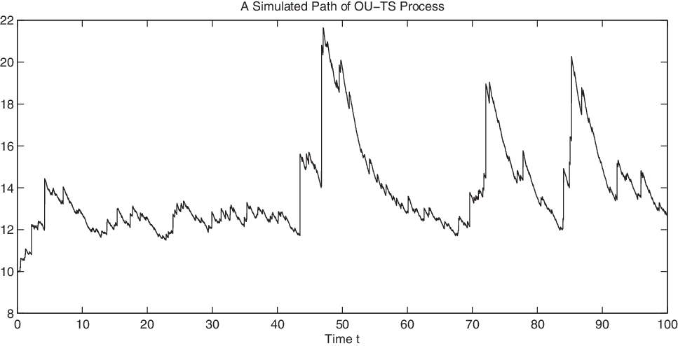
A simulated path of the OU-TS process by Algorithm 3.2, with the parameter setting $(\delta, \varrho; \alpha, \beta, \theta; X_0)=(0.2,1.0;0.9, 0.2, 0.25; 10)$ within the time period of [0,100] and 10 000 equally spaced discretisation steps.

Based on the two types of non-Gaussian OU processes defined above, the associated two types of TS-based OU processes can be naturally constructed, i.e. the so-called OU-TS process and TS-OU process, respectively. Note that we adopt the abbreviations OU-TS and TS-OU from [Reference Barndorff-Nielsen, Nicolato and Shephard11, page 13]; see also [Reference Barndorff-Nielsen and Shephard6, Reference Barndorff-Nielsen and Shephard8, Reference Barndorff-Nielsen, Jensen and SØrensen10], and [Reference Schoutens50, page 48].

Definition 2.5. (TS-based Ornstein–Uhlenbeck processes.) There are two types of TS-based Ornstein–Uhlenbeck process.

1. (i) OU-TS process. For the non-Gaussian OU process $X_t$ of Definition 2.3, if a Lévy subordinator $Z_t$ is a TS process of Definition 2.1, then $X_t$ is an OU-TS process for any time t.

2. (ii) TS-OU process. For the non-Gaussian OU process $Y_t$ of Definition 2.4, if the marginal distribution of $Y_t$ is a positive TS distribution of Definition 2.1, then $Y_t$ is a TS-OU process for any time t.

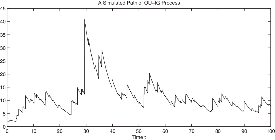
In particular, if the stable index $\alpha=1/2$ , then they reduce to OU-IG and IG-OU processes. Simulated paths of OU-TS and OU-IG processes are plotted in Figures 1 and 2, respectively.

Figure 2:

A simulated path of the OU-IG process by Algorithm 3.4, with the parameter setting $(\delta, \varrho; c; X_0)= (0.2,1.0;0.5;2.0)$ within the time period of [0,100] and 10 000 equally spaced discretisation steps.

OU-TS and TS-OU processes are very tractable, which could facilitate many types of positive time series, such as stochastic volatilities, interest rates, and default intensities. However, most of the literature concentrates on the second type, whereas in this paper we focus on the first type. Meanwhile we provide some important connections between the two.

3. Exact simulation of the OU-TS process

In this section we develop the exact simulation scheme for the OU-TS process based on the exact distributional decomposition, that is, conditional on the value of the OU-TS process at time $t\in \mathbb{R}^+$ , the distribution of the OU-TS process at time $t+\tau$ for any time lag $\tau \in \mathbb{R}^+$ can be broken into three simple elements: one constant, one TS random variable, and one compound Poisson random variable, and each of them can be exactly generated. This is achieved by the identification through the conditional Laplace transforms derived as follows.

Proposition 3.1. For a general non-Gaussian OU process $X_t$ of Definition 2.2, the Laplace transform of $ X_{t+\tau}$ conditional on $X_t$ is given by

(3.1) \begin{equation}\mathbb{E}\big[{\text{e}}^{-v X_{t+\tau} } \mid X_t \big]={\text{e}}^{-v w X_t}\times\exp\biggl(-\dfrac{\varrho}{\delta} \int_{v w}^v \dfrac{\Phi(u)}{u}\,{\text{d}} u \biggr), \quad \tau \in \mathbb{R}^+,\end{equation}

where $w\,{:}\,{\raise-1.5pt{=}}\, {\text{e}}^{-\delta \tau}$ and $\Phi(u)$ is the Laplace exponent of Lévy subordinator $Z_t$ .

Proof. Note that in general the Laplace exponent for $Z_t$ is

\[\Phi(u)=\int_0^\infty (1 - {\text{e}}^{-u y} ) \nu({\text{d}} y),\]

where $\nu$ is the Lévy measure of $Z_t$ . The infinitesimal generator $\mathcal{A}$ of process $ (X_t, t)$ acting on any function f(x, t) within its domain $\Omega (\mathcal{A})$ is given by

(3.2) \begin{equation}\mathcal{A}f (x, t)=\dfrac{\partial f}{\partial t} - \delta x \dfrac{\partial f}{\partial x} + \varrho\biggl( \int_0 ^ \infty [f( x + y, t) - f(x,t)]\nu({\text{d}} y) \biggr),\end{equation}

where $\Omega(\mathcal{A})$ is the domain for the generator $\mathcal{A}$ such that f(x,t) is differentiable with respect to x and t for all x and t, and

\[\biggl| \int_0 ^ \infty [f( x + y, t) - f(x,t)]\nu({\text{d}} y) \biggr| < \infty.\]

By applying the piecewise deterministic Markov processes theory [Reference Davis23] and martingale approach [Reference Dassios and Embrechts16], we can derive the conditional Laplace transform for $X_t$ . More precisely, set $\mathcal{A} f( x, t)=0$ ; we find a martingale

(3.3) \begin{equation}\exp\!(- X_t k \,{\text{e}}^{ \delta t})\exp\biggl(\varrho \int_0^t \Phi(k \,{\text{e}}^{\delta s}) \,{\text{d}} s \biggr) \quad \text{for all } k\in \mathbb{R}^+,\end{equation}

for which the proof is given in Appendix A. By the martingale property and setting $k=v\,{\text{e}}^{ -\delta(t+\tau)}$ , we obtain

\begin{align*} \mathbb{E}[{\text{e}}^{-v X _ {t+\tau}} \mid X _ t] &= \exp\!(-v \,{\text{e}}^ {-\delta \tau} X_t )\exp\biggl( -\varrho\int_t^ {t+\tau} \Phi ( v \,{\text{e}}^{-\delta (t+\tau -s )})\,{\text{d}} s \biggr)\\ &= \exp\!(-v \,{\text{e}}^ {-\delta \tau} X_t ) \exp\biggl(-\dfrac{\varrho}{\delta}\int_{v \,{\text{e}}^ {-\delta \tau}} ^{v} \dfrac{\Phi(u)}{u}\,{\text{d}} u\biggr).\end{align*}

The conditional Laplace transform (3.1) in Proposition 3.1 is the key tool to develop our exact simulation scheme later in this section. An alternative proof of this result via the characteristic function of the stochastic integral for a continuous function proposed by [Reference Lukacs38] can also be found in [Reference Wolfe54]. It can also be used to obtain an analytical formula for the associated conditional expectation in Proposition 3.2.

Proposition 3.2. The expectation of $X_{t+\tau}$ conditional on $X_t$ is given by

(3.4) \begin{equation}\mathbb{E}[ X_{t+\tau} \mid X_t ]=w X_t+ \dfrac{\varrho}{\delta} (1- w)\mathbb{E}[Z_1], \quad \tau \in \mathbb{R}^+,\end{equation}

where $\mathbb{E}[Z_1]=\int_0 ^ \infty s\nu({\text{d}} s)$ .

Proof. Based on Proposition 3.1, we have

\begin{align*}\mathbb{E}[ X_{t+\tau} \mid X_t ]&= -\dfrac{\partial}{\partial v} \mathbb{E}[ {\text{e}}^{-v X_{t+\tau}} \mid X_t ]\bigg|_{v=0} \\ &= {\text{e}}^{-\delta \tau} X_t+ \dfrac{\varrho}{\delta} \lim_{v \rightarrow 0} \big( \Phi^{\prime}(v)-\Phi^{\prime} \big({\text{e}}^{-\delta\tau}v \big) \big)\\ &={\text{e}}^{-\delta\tau} X_t + \dfrac{\varrho}{\delta} \lim_{v \rightarrow 0}\biggl(\int_0^\infty s \,{\text{e}}^{-vs} \nu({\text{d}} s) - w\int_0^\infty s \,{\text{e}}^{-wvs} \nu({\text{d}} s) \biggr)\\&={\text{e}}^{-\delta \tau} X_t + \dfrac{\varrho}{\delta} \big( 1 - {\text{e}}^{-\delta\tau} \big) \int_0 ^ \infty s\nu({\text{d}} s).\hfill\end{align*}

In particular, for the OU-TS process we have $\mathbb{E}[Z_1] = \theta \beta ^ {1-\alpha} \Gamma(1-\alpha)$ , where $\Gamma(\cdot)$ is a gamma function, i.e. $\Gamma(u)\,:\!=\, \int_0^\infty s^{u-1} \,{\text{e}}^{-s}\,{\text{d}} s$ . Set $t=0$ and $\tau=T>0$ in (3.4); we have

(3.5) \begin{equation}\mathbb{E}[ X_T \mid X_0 ]=X_0 \,{\text{e}}^{-\delta T}+\dfrac{\varrho}{\delta} \big(1- \,{\text{e}}^{-\delta T}\big)\theta\beta^{\alpha-1}\Gamma(1-\alpha),\end{equation}

which will be used later for numerically validating our simulation scheme in Section 5.

3.1. Simulation algorithm for the OU-TS process

The conditional distribution of an OU-TS process is decomposable, due to the infinite divisibility property of TS distribution. We choose a ‘cutting’ value to break the OU-TS process into several simple elements such that each one can be exactly simulated. Theorem 3.1 illustrates the exact distributional decomposition of an OU-TS process via integral transforms.

Theorem 3.1. For the OU-TS process $X_t$ of Definition 2.5, the Laplace transform of $X_{t+\tau}$ conditional on $X_t$ can be expressed by

\begin{align*} & \mathbb{E}\big[{\text{e}}^ {-v X_{t+\tau}} \mid X_t\big] \\ & ={\text{e}}^{-v w X_t}\times\exp\biggl(-\dfrac{\varrho\theta(1-w^{\alpha})}{\alpha\delta}\int_{0}^{\infty}(1-{\text{e}}^{-v s})\dfrac{{\text{e}}^{-({{\beta}/{w}})s}}{s^{\alpha+1}}\,{\text{d}} s\biggr) \nonumber\\ &\times\exp\biggl(-\dfrac{\varrho\theta\beta^\alpha\Gamma(1-\alpha)D_w}{\alpha\delta}\int_{0}^{\infty}(1-{\text{e}}^{-v s})\int_{1}^{{{1}/{w}}}\dfrac{(\beta u)^{1-\alpha}}{\Gamma(1-\alpha)}s^{(1-\alpha)-1}\,{\text{e}}^{-\beta us}\dfrac{ u^{\alpha-1}-u^{-1} }{D _ w}\,{\text{d}} u\,{\text{d}} s\biggr), \nonumber\end{align*}

where $w\,{:}\,{\raise-1.5pt{=}}\, {\text{e}}^{-\delta \tau}$ and

(3.6) \begin{equation}D_w\,:\!=\, \dfrac{1}{\alpha} (w^{-\alpha} -1) + \ln w.\end{equation}

Proof. Since the Lévy measure of TS is (2.1), the Laplace exponent is specified by

\begin{equation*} \Phi(u)=\int_0 ^ \infty (1- {\text{e}}^ {-u y}) \dfrac{\theta}{y^{\alpha+1}}\,{\text{e}}^{-\beta y} \,{\text{d}} y=\dfrac{\theta\Gamma(1-\alpha) }{\alpha} [ (\beta + u ) ^\alpha - \beta ^ \alpha].\end{equation*}

Based on Proposition 3.1, we have

\begin{equation*}\mathbb{E} [{\text{e}}^ {-v X_{t+\tau}} \mid X_t]={\text{e}}^{- v w X_t}\exp\biggl(-\dfrac{\varrho}{\delta} \int_{v w} ^ {v}\dfrac{1}{u} \int _ 0 ^ \infty (1- {\text{e}}^ {-u y} )\dfrac{\theta}{y ^ {\alpha + 1}} \,{\text{e}}^ { -\beta y} \,{\text{d}} y \,{\text{d}} u \biggr),\end{equation*}

where

(3.7) \begin{align} & \int_{v w}^{v}\dfrac{1}{u}\int_{0}^{\infty} ( 1-{\text{e}}^{-uy} ) \theta y^{-\alpha-1}\,{\text{e}}^{-\beta y}\,{\text{d}} y\,{\text{d}} u\nonumber\\ & \quad = \int _ {0} ^ {\infty}\dfrac{1 - {\text{e}}^ {- v s }}{s}\int _ {s} ^ {{{s}/{w}}} \theta y^{-\alpha-1}\,{\text{e}}^{-\beta y}\,{\text{d}} y\,{\text{d}} s\nonumber\\ & \quad = \int _ {0} ^ {\infty} \dfrac{1 - {\text{e}}^ {- v s}}{s}\int _ {s} ^ {{{s}/{w}}}\dfrac{\theta}{y ^ {\alpha + 1}} \big({\text{e}}^ {-\beta({{s}/{w}})}+{\text{e}}^ {-\beta y} - {\text{e}}^ {-\beta({{s}/{w}})} \big) \,{\text{d}} y \,{\text{d}} s\nonumber\\ & \quad = \int _ {0} ^ {\infty} \dfrac{ 1 - {\text{e}}^ {- v s } } { s } \int _ {s} ^ {{{s}/{w}}} \dfrac{\theta}{ y ^ { \alpha + 1 }}\,{\text{e}}^ {- \beta ({{s}/{w}})}\,{\text{d}} y \,{\text{d}} s \notag \\ & \quad \quad +\int _ {0} ^ {\infty}\dfrac{1 - {\text{e}}^ {- v s}}{s} \int _ { s } ^ {{{s}/{w}}}\dfrac{\theta}{ y ^ {\alpha + 1}} \big({\text{e}}^ {-\beta y} - {\text{e}}^ {-\beta ({{s}/{w}})} \big)\,{\text{d}} y \,{\text{d}} s.\end{align}

Since $y<{{s}/{w}}$ , the two terms in (3.7) are both positive for any $y\in[s, {{s}/{w}}]$ . In particular, for the first term of (3.7) we have

(3.8) \begin{equation}\int _ {0} ^ {\infty} \dfrac{ 1 - {\text{e}}^ {-v s }}{ s }\int _ {s} ^ {{{s}/{w}}} \dfrac{\theta}{y ^ {\alpha + 1}}\,{\text{e}}^ {-\beta ({{s}/{w}})} \,{\text{d}} y \,{\text{d}} s=\dfrac{\theta(1 - w ^ {\alpha})}{\alpha}\int _ {0} ^ {\infty} ( 1 - {\text{e}}^ {-v s} )\dfrac{{\text{e}}^ {- ({{\beta}/{w}}) s}}{s ^ {\alpha + 1}}\,{\text{d}} s,\end{equation}

and for the second term of (3.7) we have

(3.9) \begin{align} & \int_0 ^ \infty ( 1- {\text{e}}^ { -v s } ) \dfrac{1}{s}\int _ {s} ^ {{{s}/{w}}}\dfrac{\theta}{ y ^ { \alpha + 1}} \big( {\text{e}}^ {-\beta y} - {\text{e}}^ {- \beta ({{s}/{w}})} \big)\,{\text{d}} y \,{\text{d}} s \nonumber\\ & \quad = \theta\int_0 ^ \infty ( 1 - {\text{e}}^ {-v s} )\int_{1}^{{{1}/{w}}}s^{-\alpha}x^{-\alpha-1}\dfrac{{\text{e}}^{-\beta sx}-{\text{e}}^{-\beta({{s}/{w}})}}{s} \,{\text{d}} x\,{\text{d}} s \nonumber\\ & \quad =\theta\int_0 ^ \infty ( 1- {\text{e}}^ { -v s} )\int_{1}^{{{1}/{w}}}x ^ {-\alpha-1} s ^ {-\alpha}\int_{x} ^ {{{1}/{w}}} \beta \,{\text{e}}^ {-\beta su}\,{\text{d}} u \,{\text{d}} x \,{\text{d}} s\nonumber\\ & \quad = \theta\int_0 ^ \infty ( 1- {\text{e}}^ { -v s} )\int_1^{{{1}/{w}}}s^{-\alpha}\beta \,{\text{e}}^{-\beta su}\int_1 ^ u x ^ {-\alpha - 1}\,{\text{d}} x\,{\text{d}} u\,{\text{d}} s \nonumber\\ & \quad =\dfrac{ \theta \beta ^ \alpha}{\alpha}\Gamma( 1 - \alpha) D _ w \int _ 0 ^ \infty ( 1- {\text{e}}^ { -v s } )\int_{1} ^ { {{1}/{w}} }\dfrac{(\beta u) ^ { 1 - \alpha }}{\Gamma( 1 - \alpha )} s ^ { (1 - \alpha) - 1 } \,{\text{e}}^ {-\beta u s}\dfrac{1}{D _ w} \big(u ^ {\alpha - 1} - u ^ {-1} \big)\,{\text{d}} u\,{\text{d}} s,\end{align}

where

\begin{equation*} D_w = \int_1^{{{1}/{w}}} \big(u ^ {\alpha - 1} - u ^ {-1} \big)\,{\text{d}} u=\dfrac{1}{\alpha} (w^{-\alpha} -1) + \ln w.\end{equation*}

The exact distributional decomposition of $X_{t+\tau}$ conditional on $X_t$ can be immediately identified from the representation of Laplace transforms in Theorem 3.1, and hence implies an exact simulation scheme summarised in Algorithm 3.2.

Algorithm 3.2. (Exact simulation for OU-TS process.) The distribution of $X_{t+\tau}$ conditional on $X_t$ can be exactly decomposed by

\[X_{t+\tau} \mid X_t \,{\buildrel \mathcal{D} \over =}\,w X_t+ \widetilde{TS}+\sum^N_{i=1} S_i, \quad \tau \in \mathbb{R}^+,\]

where $w\,:\!=\,{\text{e}}^{-\delta \tau}$ ,

• $\widetilde{TS}$ is a TS random variable of

  (3.10) \begin{equation} \widetilde{TS} \sim \mathsf{TS}\biggl(\alpha, \, \dfrac{\beta}{w}, \, \dfrac{\varrho\theta }{\alpha\delta} (1-w^\alpha) \biggr), \end{equation}
  which can be exactly simulated by Algorithm D.1,

• N is a Poisson random variable of rate \begin{equation}({{ \varrho \theta }/{\alpha \delta}}) \beta^{\alpha} \Gamma(1-\alpha) D_w\end{equation} ,

• $\{S_i\}_{i=1,2,\ldots}$ are conditionally independent and conditionally gamma random variables of

  (3.11) \begin{equation} S_i \mid V \sim {Gamma}(1-\alpha, \, \beta V), \end{equation}
  where ${Gamma}(1-\alpha, \beta V)$ means a gamma distribution with shape parameter $(1-\alpha)$ and rate parameter $\beta V$ , given that V can be exactly simulated via Algorithm 3.3,

• $\widetilde{TS}, N$ and $\{S_i\}_{i=1,2,\ldots}$ are independent of each other.

Proof. From Theorem 3.1 we can see that the original Laplace transform has been divided into three parts, and each part is a well-defined Laplace transform. In particular, (3.8) is the Laplace transform of a TS random variable with Lévy measure

\[\nu({\text{d}} s) = \dfrac{\theta(1 - w ^ {\alpha})}{\alpha}s ^ {-\alpha - 1}\,{\text{e}}^ {- ({{\beta}/{w}}) s}\,{\text{d}} s.\]

Equation (3.9) is the Laplace transform of a compound Poisson random variable with the jump sizes following a gamma distribution of shape parameter $(1-\alpha)$ and rate parameter $\beta V$ . Here V is a well-defined random variable with density function

(3.12) \begin{equation}f_V(u) = \dfrac{1}{D _ w} \big(u ^ {\alpha - 1} - u ^ {-1} \big), \quad u\in\biggl[1,\dfrac{1}{w}\biggr].\end{equation}

Note that there are several different algorithms for generating TS random variables in the literature, such as simple stable rejection (SSR) (Algorithm D.1), double rejection [Reference Devroye24], fast rejection [Reference Hofert32], backward recursive [Reference Dassios, Qu and Zhao22], and two-dimensional single rejection [Reference Qu, Dassios and Zhao45]. The choice for the fundamental TS generator is indeed not our main focus in this paper. Here we directly adopt the SSR scheme just for the purpose of illustration. It is the simplest and most widely used algorithm for exact simulation, and it works more efficiently when $\alpha$ is larger and $\beta,\theta$ are smaller.

Algorithm 3.3. (A/R scheme for V.) The random variable V, defined by its density (3.12), can be exactly simulated via the following A/R procedure.

1. (1) Generate a candidate random variable

   (3.13) \begin{equation} E _ e \,{\buildrel \mathcal{D} \over =}\, \bigl( 1 + \sqrt{ \alpha C_w U ^ { (1) } } \bigr)^ {{{2}/{\alpha}}}, \quad U ^ {( 1 )} \sim \mathsf{U}[0,1], \end{equation}
   where
   \[ C _ w \,{:}\,{\raise-1.5pt{=}}\, \dfrac {1} {\alpha} ( w ^ {- {{\alpha}/{2}} } - 1 ) ^ 2. \]

2. (2) Generate a standard uniform random variable $U ^ {(2)} \sim \mathsf{U}[ 0 , 1]$ .

3. (3) If

   \[ U ^ {(2)} \le \dfrac{1}{2} \dfrac{ E _ e ^ \alpha - 1 } { E _ e ^ \alpha - E _ e ^ {{{ \alpha }/{2}}} }, \]
   then accept this candidate by setting $V = E_e$ ; otherwise, reject this candidate and go back to step (1).

Proof. Based on the density function (3.12), it is easy to derive the CDF of V by

\[F_{V}(u)\,:\!=\,\mathbb{P}\{ V \leq u \}=\dfrac{1}{D_w} \bigg[ \dfrac{1}{\alpha}( u^{\alpha} -1 ) - \ln u \bigg], \quad u \in\biggl[1, \dfrac{1}{w} \biggr].\]

However, its inverse function has no explicit form, and the explicit inverse transform is not available. Then it is natural to consider the A/R scheme for exact simulation. For a detailed introduction to an A/R scheme, see [Reference Asmussen and Glynn2, Reference Glasserman30]. We choose an envelope random variable $E _ e$ defined by its density function

\[ g _ e ( u )= \dfrac{1}{ C _ w }\big( u ^ { \alpha - 1} - u ^ { -{{ \alpha }/{2}} - 1 } \big), \quad u\in\biggl[1, \dfrac{1}{w} \biggr].\]

We can derive its CDF

\[G_e(u)=\dfrac {1}{ \alpha C _ w } \big( u ^ {{{\alpha}/{2}}}- 1 \big) ^ 2, \quad u\in\biggl[1, \dfrac{1}{w} \biggr],\]

which can be inverted explicitly by

\[G _ e^ { - 1 } ( x )=\bigl( 1 + \sqrt{ \alpha C _ w x } \bigr) ^ { {{2}/{ \alpha }} }, \quad x \in [0, 1 ].\]

Hence $E _ e $ can be exactly simulated by explicit inverse transform (3.13). Obviously,

\[\frac{ u ^ {\alpha } -1}{ u ^ {\alpha} - u ^ {{{\alpha}/{2}}} }\]

is a strictly decreasing function of $u\in[1, {{1}/{w}} ]$ . By L’Hôpital’s rule, we can find its upper bound

\[\lim_ { u \downarrow 1 } \dfrac{ u^ \alpha - 1 }{ u ^ {\alpha} - u ^ {{{\alpha}/{2}}} } = 2.\]

Then we have

(3.14) \begin{equation}\dfrac{ f _ V ( u ) } { g _ e ( u ) }=\dfrac{C _ w}{D _ w} \dfrac{ u ^ {\alpha} - 1 }{ u ^ {\alpha} - u ^ {{{\alpha}/{2}}} }\le\dfrac{C _ w}{D _ w}\mathop {\lim }\limits_{u \downarrow 1} \dfrac{ u ^ {\alpha} - 1 }{ u ^ {\alpha} - u ^ {{{\alpha}/{2}}} }=2 \dfrac{ C _ w } { D _ w }\,:\!=\,\bar{c} _ w \quad \text{for all}\ u \in \biggl[ 1, \dfrac {1} {w} \biggr].\end{equation}

Remark 3.1. Note that $\bar{c}_w$ of (3.14) is the expected number of candidates generated until one is accepted, hence $1/\bar{c}_w$ is the acceptance probability, i.e. the probability of acceptance on each attempt. Obviously it is preferable for us to have $\bar{c}_w$ close to 1. In fact our Algorithm 3.3 is pretty efficient, as we can prove in Appendix B that the acceptance probability is guaranteed to be above 50%. More precisely, we have $\bar{c}_w\in(1,2)$ and

(3.15) \begin{equation}\begin{cases}\bar{c}_w \to 1 & \text{when $ w\to 1$,}\\\bar{c}_w \to 2 & \text{when $ w\to 0$.}\end{cases}\end{equation}

3.2. Algorithm for the OU-IG process

We provide a tailored algorithm for a special case of an OU-IG process. The enhancement is mainly achieved by replacing the TS random variable of (3.10) in Algorithm 3.2 with an IG random variable. Mathematical properties of IG distributions are well documented in [Reference Chhikara and Folks15], and it is well known that IG random variables can be very efficiently simulated without A/R using the classical algorithm developed by [Reference Michael, Schucany and Haas41].

Algorithm 3.4. (Algorithm for OU-IG process.) For the OU process $X_t$ with Lévy subordinator $Z_t\sim \mathsf{IG}({{t}/{c}},t^2)$ , $c\in \mathbb{R}^+$ , we can exactly simulate $X_{T+\tau}$ conditional on $X_t$ via modifying Algorithm 3.2 by

1. (1) setting $\alpha=\frac{1}{2}$ , $\beta=\frac{1}{2}c^2$ , and $\theta = {(2 \pi)^{-1/2}}$ ,

2. (2) replacing the general TS random variable (3.10) with the IG random variable

   \[\widetilde{IG}\sim\mathsf{IG}\biggl(\mu_{\mathsf{IG}}= \dfrac{2\varrho}{\delta c}(\sqrt{w}-w), \, \lambda_{\mathsf{IG}} = \biggl[ \dfrac{2\varrho}{\delta }(1-\sqrt{w} ) \biggr]^2 \biggr),\]
   where $\mu_{\mathsf{IG}}$ is the mean parameter and $\lambda_{\mathsf{IG}}$ is the rate parameter.

Proof. For an IG random variable $IG\sim \mathsf{IG}({{1}/{c}},1)$ , the Lévy measure is given by

\[\nu({\text{d}} s) = \dfrac{1}{\sqrt{2\pi s ^3} } \,{\text{e}}^{-({{c^2}/{2}})s}\,{\text{d}} s,\]

and then we have

\[IG \sim \mathsf{TS}\biggl( \dfrac{1}{2}, \, \dfrac{c^2}{2}, \, \dfrac{1}{\sqrt{2\pi}}\biggr).\]

If we set $\alpha=\frac{1}{2}$ , $\beta=\frac{1}{2}c^2$ , and $\theta={(2 \pi)^{-1/2}}$ , then it recovers the special case of an OU-IG process. In particular, (3.10) turns out to be

\[\mathsf{TS}\biggl(\dfrac{1}{2}, \, \dfrac{c^2}{2w}, \, \dfrac{2\varrho}{\delta\sqrt{2\pi}} (1-\sqrt{w} )\biggr),\]

with the associated Laplace exponent

\[\int_0 ^\infty ( 1-{\text{e}}^{-vs})\dfrac{{{(2\varrho(1-\sqrt{w}))}/{\delta}}}{\sqrt{2\pi s^3}} \,{\text{e}}^{-({{({{c}/{\sqrt{w}}})^2}/{2}}) s}\,{\text{d}} s.\]

Note that in general the Laplace exponent of $\mathsf{IG} (\mu_{\mathsf{IG}}, \lambda_{\mathsf{IG}})$ is given by

(3.16) \begin{equation}\int_0^\infty (1-{\text{e}}^{-vs}) \dfrac{\sqrt{\lambda_{\mathsf{IG}}}}{\sqrt{2\pi s^3}} \,{\text{e}}^{-({{({{\sqrt{\lambda_{\mathsf{IG}}}}/{\mu_{\mathsf{IG}}}})^2}/{2}})s}\,{\text{d}} s, \quad \mu_{\mathsf{IG}}, \lambda_{\mathsf{IG}} \in \mathbb{R}^+.\end{equation}

Under the parameter setting of $\alpha=\frac{1}{2}$ , $\beta=\frac{1}{2}c^2$ , and $\theta={(2 \pi)^{-1/2}}$ , the general TS random variable in (3.10) can be replaced by an IG random variable as

\begin{equation*}\mathsf{TS}\biggl( \dfrac{1}{2}, \, \dfrac{c^2}{2w}, \, \dfrac{2\varrho}{\delta\sqrt{2\pi}}(1-\sqrt{w})\biggr) \,{\buildrel \mathcal{D} \over =}\,\mathsf{IG}\biggl(\dfrac{2\varrho}{\delta c}(\sqrt{w}-w), \, \biggl[ \dfrac{2\varrho}{\delta }(1-\sqrt{w} ) \biggr]^2 \biggr).\end{equation*}

4. Exact simulation of the TS-OU process

In this section we extend our approach developed in Section 3 to the TS-OU process $Y_t$ of Definition 2.2. Analogous to Proposition 3.1 for the OU-TS process $X_t$ , the conditional Laplace transform of the TS-OU process $Y_t$ is given by

(4.1) \begin{equation}\mathbb{E}\big[{\text{e}}^{-v Y_{t+\tau} }\mid Y_t \big]={\text{e}}^{-v w Y_t}\times\exp\biggl(- \int_{v w}^v \dfrac{\Phi(u)}{u}\,{\text{d}} u \biggr).\end{equation}

According to the general theory of OU processes [Reference Barndorff-Nielsen and Shephard5, page 173], the stationary TS-OU process $Y_t$ has a TS marginal law with Lévy measure $\nu_{\mathsf{TS}}({\text{d}} y)$ specified in (2.1). The one-dimensional distributions of the process are self-decomposable, and the Laplace exponent $\Phi(u)$ in (4.1) is of the form

\[ \Phi(u) = \int_0^\infty ( 1-{\text{e}}^{-ur})\nu_{\mathsf{BDLP}}({\text{d}} r), \]

with

(4.2) \begin{equation}\nu_{\mathsf{BDLP}}({\text{d}} r)=-\nu_{\mathsf{TS}}({\text{d}} r) - r \dfrac{\partial}{\partial r}\nu_{\mathsf{TS}}({\text{d}} r)= ( \alpha r^{-1}+\beta ) \theta r^{-\alpha} \,{\text{e}}^{-\beta r} \,{\text{d}} r,\end{equation}

where $\nu_{\mathsf{BDLP}}({\text{d}} r)$ is the Lévy measure of BDLP $R_t$ in (2.3).

Given the Lévy measure of $R_t$ , we provide the conditional expectation of $Y_{t}$ as follows.

Proposition 4.1. The expectation of $Y_{t+\tau}$ conditional on $Y_t$ is given by

(4.3) \begin{align}\mathbb{E}[ Y_{t+\tau}\mid Y_t ]&=w Y_t + (1 - w) \theta \beta ^{\alpha-1} \Gamma(1-\alpha), \end{align}

(4.4) \begin{align}\lim_{\tau\to\infty} \mathbb{E}[ Y_{t+\tau}\mid Y_t ]&= \theta \beta ^{1-\alpha} \Gamma(1-\alpha).\end{align}

Proof. Based on (4.2), (4.3) can be immediately derived from (3.4) by

\[\int_0 ^ \infty s \nu_{\mathsf{BDLP}}({\text{d}} s)=\alpha \theta \beta ^{\alpha-1}\Gamma(1-\alpha) +\theta \beta^{\alpha -1} \Gamma(2-\alpha).\]

Take the limit of $\tau\to\infty$ for (4.3), then $w \rightarrow 0$ and we have (4.4).

In fact we can see from (4.2) that the Lévy measure of the BDLP of a TS-OU process is the sum of Lévy measures of a TS process and a compound Poisson process. Hence, based on the exact decomposition of an OU-TS process in Algorithm 3.2, the distribution of a TS-OU process at a given time is equivalent to the sum of a TS random variable and two compound Poisson random variables, as specified by Algorithm 4.1, with the proof outlined in Appendix C.

Algorithm 4.1. (Exact simulation for TS-OU process.) The distribution of $Y_{T+\tau}$ conditional on $Y_t$ can be exactly decomposed as

\begin{equation*} Y_{t+\tau} \mid Y_t \,{\buildrel \mathcal{D} \over =}\,wY_t + \breve{\widetilde{TS}} + \sum_ {i=1} ^ { \tilde{N} } {S}_i +\sum_ {j=1} ^ {\breve{N}} \breve{S}_j, \quad \tau \in \mathbb{R}^+,\end{equation*}

where $w\,:\!=\,{\text{e}}^{-\delta \tau}$ ,

• \begin{equation}\breve{\widetilde{TS}}\end{equation} is a TS random variable of

  (4.5) \begin{equation} \breve{\widetilde{TS}} \sim \mathsf{TS}\biggl( \alpha, \, \dfrac{\beta}{w}, \, \theta (1-w^\alpha) \biggr){,} \end{equation}

• $\tilde{N}$ is a Poisson random variable of rate $\theta \beta^{\alpha} \Gamma(1-\alpha) D_w$ , and the jump sizes $\{S_i\}_{i=1,2,\ldots}$ are i.i.d. and exactly the same as (3.11),

• $\breve{N}$ is another Poisson random variable of rate $ \theta\beta^\alpha \Gamma(1-\alpha) \ln ({{1}/{w}} )$ , and the jump sizes $\{\breve{S} _ j \} _ {j=1,2,\ldots}$ are conditionally independent and conditionally gamma random variables of

  \[ \breve{S}_j \mid V^* \sim {Gamma} (1-\alpha, \, \beta V^* ), \]
  given that
  (4.6) \begin{equation} V^* \,{\buildrel \mathcal{D} \over =}\, \exp ( \delta\tau U^{(3)} ), \quad U^{(3)}\sim \mathsf{U}[0,1]{,}\end{equation}

• $\breve{\widetilde{TS}},\tilde{N},\breve{N}$ , $\{S_i\}_{i=1,2,\ldots}$ and $\{\breve{S} _ j \} _ {j=1,2,\ldots}$ are independent of each other.

Accordingly, we also offer a tailored scheme for the IG-OU process.

Proof. When $\alpha=\frac{1}{2}$ , $\beta=\frac{1}{2}c^2$ , and $\theta={(2 \pi)^{-1/2}}$ , the Laplace exponent of (4.5) is

\[\int_0^\infty (1 - {\text{e}}^{-v s}) \dfrac{ 1-\sqrt{w}}{\sqrt{2\pi s^3}} \,{\text{e}}^ {-({{({{c}/{\sqrt{w}}})^2}/{2}})s}\,{\text{d}} s.\]

Comparing with (3.16), we have

\begin{equation*}\mathsf{TS}\biggl(\dfrac{1}{2},\, \dfrac{c^2}{2w}, \,\theta(1-\sqrt{w})\biggr) \,{\buildrel \mathcal{D} \over =}\,\mathsf{IG}\biggl(\dfrac{1}{c} (\sqrt{w}-w), \, ( 1-\sqrt{w} )^2 \biggr).\end{equation*}

5. Numerical examples

In this section we illustrate the performance and effectiveness of our exact simulation schemes via extensive numerical experiments. We have implemented the exact simulation scheme for four cases, OU-TS/OU-IG and TS-OU/IG-OU processes within the fixed time period [0, T], respectively. They are mainly implemented on a desktop with an Intel Core i7-6700 CPU@3.40GHz processor, 24.00GB RAM, Windows 10 Professional, 64-bit Operating System. The algorithms are coded and performed in MATLAB^® (R2012a), and the computing time is measured by the elapsed CPU time in seconds. We use our algorithms to simulate paths of $X_t$ and $Y_t$ from time 0 to T, and numerically validate and test them based on the true values of means (3.5) and (4.3) at the terminal time T for OU-TS/OU-IG processes and TS-OU/IG-OU processes, respectively. The associated errors from the true values are reported by three standard measures:

1. (i) ${\it difference} = \text{estimated value} - \text{true value}$ ,

2. (ii) ${\it relative error (error %)} = \dfrac{\text{estimated value} - \text{true value}}{\text{true value}}$ ,

3. (iii) root mean square error $\text{RMSE}=\sqrt{\text{bias}^2 + \text{SE}^2}$ , where the SE is the standard error of the simulation output, and the bias is the difference between the expectation of the estimator and the associated true (theoretical) value. For our exact simulation schemes, the bias is zero.

We set the parameters $(\delta, \varrho; \alpha, \beta, \theta; X_0=Y_0; T)=(0.2, 1.0; 0.25, 0.5, 0.25; 10.0; 5.0)$ for OU-TS/TS-OU processes and $(\delta, \varrho; c; X_0=Y_0; T)= (0.2, 1.0; 1.0; 10.0; 5.0)$ for OU-IG/IG-OU processes, and experiment with different numbers of equally spaced discretisation steps within the period [0,T], i.e. $n_{\tau}\,:\!=\,T/\tau$ . Of course, all of our algorithms can be directly applied to the irregularly spaced time points which may be more useful in practice, as the data, such as trade transactions from market microstructure, are often observed at irregularly spaced time points (see [Reference Engle and Russell27]), but the equally spaced cases here just serve for the purpose of illustration.

Table 1

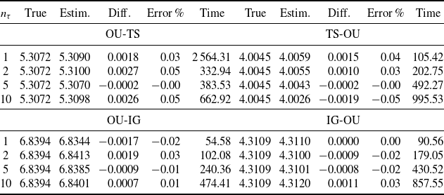
Comparison between the true means and the associated simulation results of our exact simulation schemes for 1 024 000 replications, based on the parameter setting $(\delta, \varrho; \alpha, \beta, \theta; X_0=Y_0; T)=(0.2, 1.0; 0.25, 0.5, 0.25; 10.0; 5.0)$ for OU-TS/TS-OU processes and $(\delta, \varrho; c; X_0=Y_0; T) = (0.2, 1.0; 1.0; 10.0; 5.0)$ for OU-IG/IG-OU processes with $n_\tau=1,2,5,10$ , respectively.

Table 2

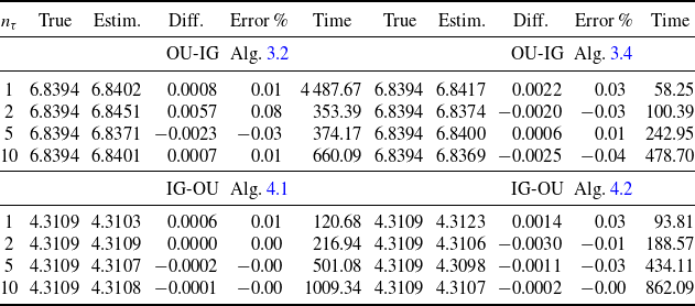
Comparison between the true means and the associated simulation results of our exact simulation schemes for 1 024 000 replications, based on the parameter setting $(\delta, \varrho; c; X_0=Y_0; T)= (0.2, 1.0; 1.0; 10.0; 5.0)$ for OU-IG/IG-OU processes with $n_\tau=1,2,5,10$ , respectively.

Simulated paths of OU-TS/OU-IG processes were presented earlier in Figures 1 and 2, respectively. Numerical verification for the four cases, OU-TS/TS-OU, OU-IG/IG-OU, are reported in Table 1. The efficiency enhancement for simulating OU-IG/IG-OU processes using the tailored schemes (Algorithms 3.4 and 4.2) against the associated general schemes (Algorithms 3.2 and 4.1) can be clearly observed via numerical results reported in Table 2. Overall, from the numerical results reported in this section, it is evident that each algorithm developed in this paper can achieve a very high level of accuracy as well as efficiency.

The conditional mean provides us with the easiest way to test and verify newly developed algorithms, as its true value can be much easier to derive in a simple analytic form in most circumstances, as given by (3.5) and (4.3). In fact our tests and validations based on the means have been carried out using a vast number of various different parameter sets. The results based on other parameter sets show very similar levels of accuracy and efficiency, so in order to make our presentation more concise we do not present all of them here. Of course, other higher moments, values of probabilities, or density functions can be also convenient to use for testing as long as they have analytic forms so that we already know the true values precisely. For example, the conditional Laplace transforms we derived in Proposition 3.1 and Theorem 3.1 could be used for testing as well. But we first have to discretise and truncate the infinite integrals in the Laplace transforms, which would introduce estimation errors. Basically, means can be tested by a sufficient number of different parameter choices. The aim of testing and verifying our algorithms numerically can be achieved similarly, based on the simple mean and higher moments, so we choose means for simplicity and also avoid additional estimation errors.

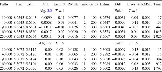
Alternatively, a widely used and simpler approach for simulating stochastic processes is the Euler time-discretisation scheme. However, it is well known that this scheme is not exact and it introduces biases for the estimators. For example, the continuous-time OU-TS process $X_t$ following the SDE (2.2) can be approximated by $\hat{X}_t$ via the Euler discretisation scheme

\[\hat{X}_{t+h} - \hat{X}_t = -\delta \hat{X}_t h + \varrho (Z_{t+h} - Z_t),\]

or

\[\hat{X}_{t+h} = (1 -\delta h) \hat{X}_t + \varrho (Z_{t+h} - Z_t), \quad h = T/n_{g},\]

where $n_{g} \in \mathbb{N}^+$ is the total number of grids within the time interval [0,T], and $(Z_{t+h} - Z_t) \sim \mathsf{TS} (\alpha, \beta,\theta h )$ . According to the principle of optimal allocation of computation budget proposed by [Reference Duffie and Glynn25], the number of time-discretisation grids is set equal to the square root of the number of sample paths, i.e. $n_{g}=\sqrt{n_p}$ , where $n_p$ is the total number of sample paths. 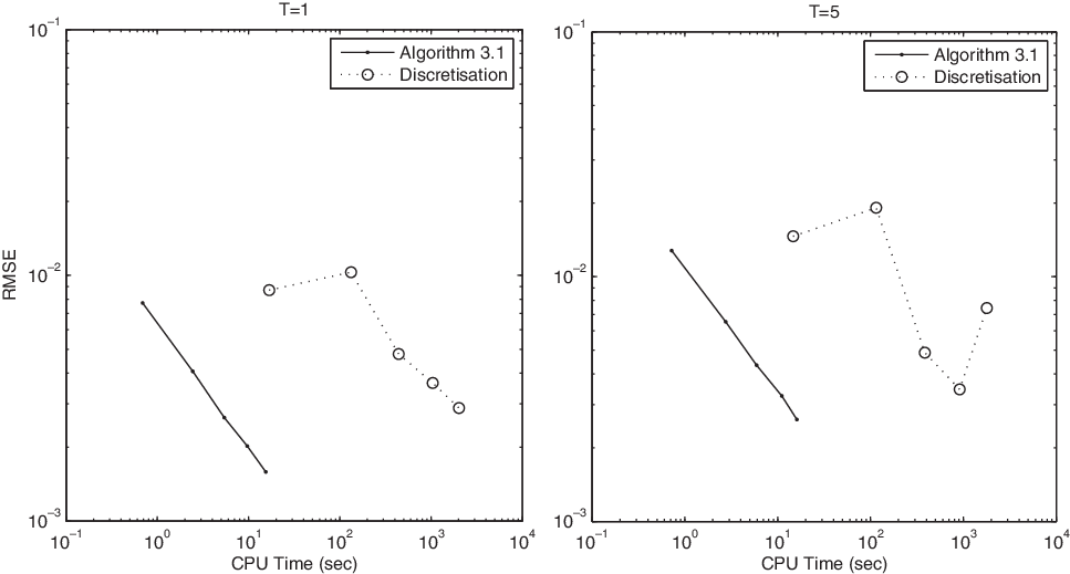The comparison results between Algorithm 3.2 and the Euler discretisation scheme for the OU-TS process, based on the parameter setting $(\delta, \varrho; \alpha, \beta, \theta; X_0)=(0.2, 1.0; 0.25, 0.5, 0.25; 10.0)$ and $T=1,5$ , are reported in Table 3 with convergence comparison in Figure 3. Obviously, our algorithm outperforms the discretisation scheme in terms of RMSE and CPU time. In conclusion, our exact simulation scheme is far more efficient and accurate than the Euler discretisation scheme.

Table 3

Comparison between the true means and the associated simulation results for Algorithm 3.2 and discretisation scheme for the OU-TS process, based on the parameter setting $(\delta, \varrho; \alpha, \beta, \theta; X_0)=(0.2, 1.0; 0.25, 0.5, 0.25; 10.0)$ and $T=1,5$ , respectively, with the associated plots provided in Figure 3.

Figure 3:

Convergence comparison between Algorithm 3.2 and discretisation scheme for the OU-TS process, based on the parameter setting $(\delta, \varrho; \alpha, \beta, \theta; X_0)=(0.2, 1.0; 0.25, 0.5, 0.25; 10.0)$ and $T=1,5$ , respectively, with the associated detailed numerical results reported in Table 3.

6. Extensions

Based on the results proposed in Section 3, one could further decompose certain types of Lévy-driven OU processes with the BDLPs beyond tempered stable processes. The details are provided in Proposition 6.1.

Proposition 6.1. Let $X_t$ be a non-Gaussian OU process of Definition 2.3, and the Lévy measure of the BDLP $Z_t$ is of the form

(6.1) \begin{equation}\nu({\text{d}} y)=\dfrac{\theta h(y)}{y^{\alpha+1} }\,{\text{d}} y,\end{equation}

where $\nu$ satisfies the following condition:

\[\int_0^\infty \min\{ 1, y\}\nu({\text{d}} y)<\infty.\]

For the following two cases, the distribution of $X_{t+\tau} $ conditional on $X_t$ can be exactly decomposed.

Case I. If

(6.2) \begin{equation} \hat{D}_w \,{:}\,{\raise-1.5pt{=}}\, \int_0^\infty \int_1^{{{1}/{w}}} \dfrac{h(su)-h({{s}/{w}}) }{ s^{\alpha+1}u^{\alpha+1}}\,{\text{d}} u\,{\text{d}} s <\infty \end{equation}

and $w\,{:}\,{\raise-1.5pt{=}}\, {\text{e}}^{-\delta \tau}$ , then $X_{t+\tau}\mid X_t$ can be expressed as

\[ X_{t+\tau}\mid X_t \,{\buildrel \mathcal{D} \over =}\, wX_t + w \hat{Z} +\sum_{i=1}^{\hat{N} } \hat{S}_i, \quad \tau\in\mathbb{R}^+, \]

where

• $\hat{Z}$ is a Lévy subordinator with Lévy measure

  \[ \nu({\text{d}} s) = \dfrac{ \varrho\theta(1/w^\alpha-1)}{\alpha\delta} \dfrac{h(s)}{s^{\alpha+1}} \,{\text{d}} s{,} \]

• $\hat{N}$ is a Poisson random variable of rate ${{ \varrho\theta\hat{D}_w}/{\delta}}$ ,

• $\{\hat{S_i}\}_{i=1,2,\ldots}$ are i.i.d. random variables with density

  \[ f_{\hat{S}}(s)= \dfrac{1}{\hat{D}_w} \int_1^{{{1}/{w}}} \dfrac{h(su)-h({{s}/{w}}) }{ s^{\alpha+1}u^{\alpha+1}}\,{\text{d}} u, \quad s\in(0,\infty){,} \]

• $\hat{Z}$ , $\hat{N}$ , and $\{ \hat{S}_i\}_{i=1,2,\ldots}$ are independent of each other.

Case II. If $h(\cdot)$ in (6.1) satisfies the conditions

(6.3) \begin{equation}h(y)\ge {\text{e}}^{-\beta y} \quad {for\ all} \ y\in(0,\infty),\end{equation}

and

(6.4) \begin{equation}\bar{D}_w\,:\!=\,\int_0^\infty \int_1^{{{1}/{w}}} \dfrac{h(su)-{\text{e}}^{-\beta s u} }{ s^{\alpha+1} u^{\alpha+1} }\,{\text{d}} u\,{\text{d}} s <\infty,\end{equation}

and $w\,{:}\,{\raise-1.5pt{=}}\, {\text{e}}^{-\delta \tau}$ , then $X_{t+\tau}\mid X_t$ can be expressed as

\[ X_{t+\tau} \mid X_t \,{\buildrel \mathcal{D} \over =}\, w X_t + \widetilde{TS} + \sum^N_{i=1} S_i+\sum_{i=1}^{\bar{N}}\bar{S}_i, \quad \tau \in \mathbb{R}^+,\]

where

• $\widetilde{TS}$ , N, $\{S_i\}_{i=1,2,\ldots}$ are suggested in Algorithm 3.2,

• $\bar{N}$ is a Poisson random variable of rate ${{\varrho \theta \bar{D}_w}/{\delta}}$ ,

• $\{\bar{S_i}\}_{i=1,2,\ldots}$ are i.i.d. random variables with density

  \[ f_{\bar{S}}(s)= \dfrac{1}{\bar{D}_w} \int_1^{{{1}/{w}}} \dfrac{h(su)-{\text{e}}^{-\beta s u} }{ s^{\alpha+1} u^{\alpha+1} }\,{\text{d}} u, \quad s\in(0,\infty){,} \]

• $\widetilde{TS}$ , N, $\bar{N}$ , $\{S_i\}_{i=1,2,\ldots}$ and $\{\bar{S_i}\}_{i=1,2,\ldots}$ are independent of each other.

Proof. According to Proposition 3.1, the Laplace transform of $X_{t+\tau}$ conditional on $X_t$ is given by

\begin{equation*} \mathbb{E}[ {\text{e}}^{-v X_{t+\tau}}\mid X_t]={\text{e}}^{-vw X_t}\exp\biggl(-\dfrac{ \varrho\theta}{\delta} \int_0^\infty ( 1-{\text{e}}^{-vs}) \dfrac{1}{s}\int_s^{{{s}/{w}}} \dfrac{h(y)}{y^{\alpha+1}}\,{\text{d}} y\,{\text{d}} s \biggr).\end{equation*}

For Case I we have

\begin{align*}&\mathbb{E}[ {\text{e}}^{-v X_{t+\tau}}\mid X_t]\nonumber\\ & \quad ={\text{e}}^{-vw X_t}\exp\biggl(-\dfrac{ \varrho\theta}{\delta} \int_0^\infty ( 1-{\text{e}}^{-vs}) \dfrac{1}{s}\int_s^{{{s}/{w}}} \dfrac{h({{s}/{w}}) }{y^{\alpha+1}}\,{\text{d}} y\,{\text{d}} s \biggr)\notag \\ & \quad \quad \times \exp\biggl(-\dfrac{ \varrho\theta}{\delta} \int_0^\infty ( 1-{\text{e}}^{-vs}) \dfrac{1}{s}\int_s^{{{s}/{w}}} \dfrac{h(y)-h({{s}/{w}}) }{y^{\alpha+1}}\,{\text{d}} y\,{\text{d}} s \biggr)\nonumber\\& \quad ={\text{e}}^{-vw X_t}\exp\biggl(-\dfrac{ \varrho\theta(1/w^\alpha-1)}{\alpha\delta} \int_0^\infty ( 1-{\text{e}}^{-vws}) \dfrac{h(s)}{s^{\alpha+1}} \,{\text{d}} s \biggr)\nonumber\\& \quad \quad \times\exp\biggl(-\dfrac{ \varrho\theta\hat{D}_w}{\delta} \int_0^\infty ( 1-{\text{e}}^{-vs}) \int_1^{{{1}/{w}}} \dfrac{h(su)-h({{s}/{w}}) }{\hat{D}_w s^{\alpha+1}u^{\alpha+1}}\,{\text{d}} u\,{\text{d}} s \biggr),\end{align*}

where $\hat{D}_w$ is specified in (6.2). We can see that $X_{t+\tau}\mid X_t$ can be expressed as the sum of a deterministic constant, a Lévy subordinator with measure proportional to (6.1), and a compound Poisson random variable under the condition $\hat{D}_w<\infty$ .

For Case II we have

\begin{align*} &\mathbb{E}[ {\text{e}}^{-v X_{t+\tau}}\mid X_t]\nonumber\\&= {\text{e}}^{-vw X_t}\exp\biggl(-\dfrac{ \varrho\theta}{\delta} \int_0^\infty ( 1-{\text{e}}^{-vs}) \dfrac{1}{s}\int_s^{{{s}/{w}}} \dfrac{{\text{e}}^{-\beta y} }{y^{\alpha+1}}\,{\text{d}} y\,{\text{d}} s \biggr)\\ & \times \exp\biggl(-\dfrac{ \varrho\theta}{\delta} \int_0^\infty ( 1-{\text{e}}^{-vs}) \dfrac{1}{s}\int_s^{{{s}/{w}}} \dfrac{h(y)-{\text{e}}^{-\beta y} }{y^{\alpha+1}}\,{\text{d}} y\,{\text{d}} s \biggr)\nonumber\\&={\text{e}}^{-vw X_t}\exp\biggl(-\dfrac{\varrho\theta(1-w^{\alpha})}{\alpha\delta}\int_{0}^{\infty}(1-{\text{e}}^{-v s})\dfrac{{\text{e}}^{-{{\beta}/{w}}s}}{s^{\alpha+1}}\,{\text{d}} s\biggr) \nonumber\\& \times\exp\biggl(-\dfrac{\varrho\theta\beta^\alpha\Gamma(1-\alpha)D_w}{\alpha\delta}\int_{0}^{\infty}(1-{\text{e}}^{-v s})\int_{1}^{{{1}/{w}}}\dfrac{(\beta u)^{1-\alpha}}{\Gamma(1-\alpha)}s^{(1-\alpha)-1}\,{\text{e}}^{-\beta us}\dfrac{ u^{\alpha-1}-u^{-1} }{D _ w}\,{\text{d}} u\,{\text{d}} s\biggr)\nonumber\\& \times\exp\biggl(-\dfrac{\varrho\theta \bar{D}_w}{\delta} \int_0^\infty ( 1-{\text{e}}^{-vs}) \int_1^{{{1}/{w}}} \dfrac{h(su)-{\text{e}}^{-\beta s u} }{\bar{D}_w s^{\alpha+1} u^{\alpha+1} } \,{\text{d}} u\,{\text{d}} s \biggr),\end{align*}

where $D_w$ is given by (3.6) and $\bar{D}_w$ is given in (6.4). We can see that, based on the exact decomposition of the OU-TS process in Algorithm 3.2, the distribution of this new Lévy-driven OU process at a given time is equivalent to the sum of a TS random variable and two compound Poisson random variables under the conditions $h(y)\ge {\text{e}}^{-\beta y}$ for all $y\in(0,\infty)$ and $\bar{D}_w<\infty$ .

In general, when the function $h(\cdot)$ is specified, it is highly likely that the simulation scheme for the corresponding Lévy subordinator $Z_t$ is not available, and therefore one has to consider Case II. However, there are some rare cases when the simulation schemes for $Z_t$ with Lévy measure in (6.1) are indeed available. One typical example is an indicator function $h(y)=\textbf{1}_{\{0 \lt y \lt b\}}$ with b being a positive constant. The associated Lévy subordinator $Z_t$ , namely the truncated stable process, can be simulated via the exact simulation scheme proposed by [Reference Dassios, Lim and Qu21]. Hence, by ensuring the corresponding $\hat{D}_w<\infty$ , one could use the decomposition scheme above to sample this truncated stable-driven OU process. The details of the simulation procedures for this truncated stable-driven OU process are provided in [Reference Dassios, Lim and Qu21, page 22].