1 Introduction
Convective flows are of much interest to researchers from both a theoretical and practical point of view. Such interest stems from the occurrence of these flows in many geophysical and engineering fields, including solid matrix heat exchangers, ground water movement, geothermal energy extraction, oil and gas production, thermal insulation drying porous solids, nuclear waste disposal and many others. Mixed convection flows, whereby there is an interaction between an imposed flow and the internally generated buoyancy forces, are also significant in nuclear reactors, solar collectors, crystal growth and cooling electronic systems. Air cooling systems are used as primary cooling media for the efficiency of electronic systems due to being both simple in design and cost-effective in maintenance. To remove heat from these systems, both natural convection and externally forced convection have been used. The interaction between the externally induced flow and natural convection due to the buoyancy forces plays a significant role in the shape and operation of electronic systems.
Stagnation-point flows, describing the fluid motion near the stagnation region at the front of a blunt-nosed body, exists on all solid bodies moving in a fluid. The stagnation region encounters the highest pressure, the highest heat transfer and the highest rates of mass deposition. Hiemenz (Reference Hiemenz1911) was the first to study two-dimensional stagnation flows using a similarity transform to reduce the Navier–Stokes equations to nonlinear ordinary differential equations. The axisymmetric case was later solved by Homann (Reference Homann1936).
Mixed convection over flat surfaces represents another important problem, which is often encountered in the environment and in engineering devices. Therefore, the knowledge of heat transfer phenomena over this kind of geometry is also very important in developing compact and highly efficient heat exchanger components. A literature review reveals that an extensive amount of work has already been done on convection boundary-layer flow near a stagnation point on a vertical flat plate. To the best of our knowledge, no study has yet been done on the mixed convection flow on a non-axisymmetric Homann’s stagnation-point flow. From this survey, it appears that Kuiken (Reference Kuiken1969) has studied the free convection over a vertical flat plate. Merkin (Reference Merkin1989, Reference Merkin1994) has also studied problems on the free convection past a vertical flat plate. Much of this work is described in detail in the books by Gebhart et al. (Reference Gebhart, Jaluria, Mahajan and Sammakia1988), Schlichting & Gersten (Reference Schlichting and Gersten2000), Pop & Ingham (Reference Pop and Ingham2001) and Bejan (Reference Bejan2013).
Hence, given the knowledge of this previously mentioned literature, our aim is to study the mixed convection non-axisymmetric Homann stagnation-point flow over a vertical surface. This problem can be regarded as the extension of the study by Weidman (Reference Weidman2012) to include heat transfer and the effects of the induced buoyancy.
2 Problem formulation
We consider the steady mixed convection non-axisymmetric Homann stagnation-point flow (Homann Reference Homann1936) over a vertical flat wall placed in a viscous and incompressible fluid. It is assumed that the velocity components of the external flow, or potential flow, are
 $U_{e}(x,y)=(a+b)x$
,
 $V_{e}(x,y)=(a-b)y$
and
 $W_{e}(z)=-2az$
. The surface temperature is taken as
 $T_{w}(x)=T_{\infty }+T_{0}x$
. Here
 $x,y$
and
 $z$
are Cartesian coordinates, with the
 $z$
axis measured in the normal direction to the wall and the
 $x$
axis measured in the vertical direction, respectively;
 $a$
is the strain rate of the stagnation-point flow,
 $b$
is the shear rate,
 $T_{\infty }$
is the constant ambient temperature and
 $T_{0}$
is a characteristic temperature scale, with
 $T_{0}>0$
for a heated surface (aiding flow) and
 $T_{0}<0$
for a cooled surface (opposing flow).
The governing equations are, in Cartesian form (see Weidman Reference Weidman2012; Bejan Reference Bejan2013),
 $$\begin{eqnarray}\displaystyle & \displaystyle \frac{\unicode[STIX]{x2202}u}{\unicode[STIX]{x2202}x}+\frac{\unicode[STIX]{x2202}v}{\unicode[STIX]{x2202}y}+\frac{\unicode[STIX]{x2202}w}{\unicode[STIX]{x2202}z}=0, & \displaystyle\end{eqnarray}$$
 $$\begin{eqnarray}\displaystyle & \displaystyle u\frac{\unicode[STIX]{x2202}u}{\unicode[STIX]{x2202}x}+v\frac{\unicode[STIX]{x2202}u}{\unicode[STIX]{x2202}y}+w\frac{\unicode[STIX]{x2202}u}{\unicode[STIX]{x2202}z}=-\frac{1}{\unicode[STIX]{x1D70C}}\frac{\unicode[STIX]{x2202}p}{\unicode[STIX]{x2202}x}+g\unicode[STIX]{x1D6FD}(T-T_{\infty })+\unicode[STIX]{x1D708}\left(\frac{\unicode[STIX]{x2202}^{2}u}{\unicode[STIX]{x2202}x^{2}}+\frac{\unicode[STIX]{x2202}^{2}u}{\unicode[STIX]{x2202}y^{2}}+\frac{\unicode[STIX]{x2202}^{2}u}{\unicode[STIX]{x2202}z^{2}}\right), & \displaystyle\end{eqnarray}$$
 $$\begin{eqnarray}\displaystyle & \displaystyle u\frac{\unicode[STIX]{x2202}v}{\unicode[STIX]{x2202}x}+v\frac{\unicode[STIX]{x2202}v}{\unicode[STIX]{x2202}y}+w\frac{\unicode[STIX]{x2202}v}{\unicode[STIX]{x2202}z}=-\frac{1}{\unicode[STIX]{x1D70C}}\frac{\unicode[STIX]{x2202}p}{\unicode[STIX]{x2202}y}+\unicode[STIX]{x1D708}\left(\frac{\unicode[STIX]{x2202}^{2}v}{\unicode[STIX]{x2202}x^{2}}+\frac{\unicode[STIX]{x2202}^{2}v}{\unicode[STIX]{x2202}y^{2}}+\frac{\unicode[STIX]{x2202}^{2}v}{\unicode[STIX]{x2202}z^{2}}\right), & \displaystyle\end{eqnarray}$$
 $$\begin{eqnarray}\displaystyle & \displaystyle u\frac{\unicode[STIX]{x2202}w}{\unicode[STIX]{x2202}x}+v\frac{\unicode[STIX]{x2202}w}{\unicode[STIX]{x2202}y}+w\frac{\unicode[STIX]{x2202}w}{\unicode[STIX]{x2202}z}=-\frac{1}{\unicode[STIX]{x1D70C}}\frac{\unicode[STIX]{x2202}p}{\unicode[STIX]{x2202}z}+\unicode[STIX]{x1D708}\left(\frac{\unicode[STIX]{x2202}^{2}w}{\unicode[STIX]{x2202}x^{2}}+\frac{\unicode[STIX]{x2202}^{2}w}{\unicode[STIX]{x2202}y^{2}}+\frac{\unicode[STIX]{x2202}^{2}w}{\unicode[STIX]{x2202}z^{2}}\right), & \displaystyle\end{eqnarray}$$
 $$\begin{eqnarray}\displaystyle & \displaystyle u\frac{\unicode[STIX]{x2202}T}{\unicode[STIX]{x2202}x}+v\frac{\unicode[STIX]{x2202}T}{\unicode[STIX]{x2202}y}+w\frac{\unicode[STIX]{x2202}T}{\unicode[STIX]{x2202}z}=\unicode[STIX]{x1D6FC}\left(\frac{\unicode[STIX]{x2202}^{2}T}{\unicode[STIX]{x2202}x^{2}}+\frac{\unicode[STIX]{x2202}^{2}T}{\unicode[STIX]{x2202}y^{2}}+\frac{\unicode[STIX]{x2202}^{2}T}{\unicode[STIX]{x2202}z^{2}}\right), & \displaystyle\end{eqnarray}$$
subject to the boundary conditions
 $$\begin{eqnarray}\displaystyle \left.\begin{array}{@{}c@{}}\displaystyle u=v=w=0,\quad T=T_{w}\quad \text{on }z=0,\\ \displaystyle u\rightarrow U_{e},\quad v\rightarrow V_{e},\quad w\rightarrow W_{e},\quad T\rightarrow T_{\infty },\quad p\rightarrow p_{0}\quad \text{as }z\rightarrow \infty ,\end{array}\right\} & & \displaystyle\end{eqnarray}$$
where
 $u$
,
 $v$
and
 $w$
are, respectively, the velocity components along
 $x$
,
 $y$
and
 $z$
directions,
 $p$
is the fluid pressure,
 $g$
is the acceleration due to gravity,
 $\unicode[STIX]{x1D70C}$
is the constant fluid density,
 $\unicode[STIX]{x1D6FD}$
is the coefficient of thermal expansion,
 $\unicode[STIX]{x1D708}$
is the kinematic viscosity,
 $\unicode[STIX]{x1D6FC}$
is the thermal diffusivity and
 $p_{0}$
is the constant far-field pressure.
We look for similarity solutions to (2.1)–(2.6) following Weidman (Reference Weidman2012) by writing
 $$\begin{eqnarray}\displaystyle \left.\begin{array}{@{}c@{}}\displaystyle u=(a+b)xf^{\prime }(\unicode[STIX]{x1D702}),\quad v=(a-b)yg^{\prime }(\unicode[STIX]{x1D702}),\quad w=-\sqrt{\frac{\unicode[STIX]{x1D708}}{a}}((a+b)f(\unicode[STIX]{x1D702})+(a-b)g(\unicode[STIX]{x1D702})),\\ \displaystyle T-T_{\infty }=T_{0}x\unicode[STIX]{x1D703}(\unicode[STIX]{x1D702}),\quad \unicode[STIX]{x1D702}=\sqrt{\frac{a}{\unicode[STIX]{x1D708}}}z.\end{array}\right\} & & \displaystyle \nonumber\\ \displaystyle & & \displaystyle\end{eqnarray}$$
Substituting transformation (2.7) into (2.1)–(2.6), we obtain the following nonlinear ordinary differential equations,
 $$\begin{eqnarray}\displaystyle & \displaystyle f^{\prime \prime \prime }+(1+\unicode[STIX]{x1D6FE})(ff^{\prime \prime }+1-f^{\prime 2})+(1-\unicode[STIX]{x1D6FE})gf^{\prime \prime }+(1+\unicode[STIX]{x1D6FE})\unicode[STIX]{x1D706}\unicode[STIX]{x1D703}=0, & \displaystyle\end{eqnarray}$$
 $$\begin{eqnarray}\displaystyle & \displaystyle g^{\prime \prime \prime }+(1-\unicode[STIX]{x1D6FE})(gg^{\prime \prime }+1-g^{\prime 2})+(1+\unicode[STIX]{x1D6FE})fg^{\prime \prime }=0, & \displaystyle\end{eqnarray}$$
 $$\begin{eqnarray}\displaystyle & \displaystyle \frac{1}{Pr}\unicode[STIX]{x1D703}^{\prime \prime }+(1+\unicode[STIX]{x1D6FE})(f\unicode[STIX]{x1D703}^{\prime }-f^{\prime }\unicode[STIX]{x1D703})+(1-\unicode[STIX]{x1D6FE})g\unicode[STIX]{x1D703}^{\prime }=0, & \displaystyle\end{eqnarray}$$
subject to the boundary conditions
 $$\begin{eqnarray}\displaystyle \left.\begin{array}{@{}c@{}}\displaystyle f(0)=f^{\prime }(0)=0,\quad g(0)=g^{\prime }(0)=0,\quad \unicode[STIX]{x1D703}(0)=1,\\ \displaystyle f^{\prime }\rightarrow 1,g^{\prime }\rightarrow 1,\unicode[STIX]{x1D703}\rightarrow 0\text{ as }\unicode[STIX]{x1D702}\rightarrow \infty ,\end{array}\right\} & & \displaystyle\end{eqnarray}$$
where primes denote differentiation with respect to the independent variable
 $\unicode[STIX]{x1D702}$
and
 $$\begin{eqnarray}\displaystyle Pr=\frac{\unicode[STIX]{x1D708}}{\unicode[STIX]{x1D6FC}},\quad \unicode[STIX]{x1D706}=\frac{g\unicode[STIX]{x1D6FD}T_{0}}{(a+b)^{2}},\quad \unicode[STIX]{x1D6FE}=\frac{b}{a}. & & \displaystyle\end{eqnarray}$$
The parameter
 $\unicode[STIX]{x1D706}$
represents the strength of the buoyancy force relative to the shear to strain rate and is positive for aiding flow, i.e. buoyancy force in the same direction as the external forcing, or negative for opposing flow, i.e. buoyancy force in the opposite direction to the external forcing. The pressure
 $p$
is given as equation (2.15) in Weidman (Reference Weidman2012); the same result applies here since
 $T=T_{\infty }$
in the outer flow.
The main physical quantities of interest are the values of
 $f^{\prime \prime }(0)$
and
 $g^{\prime \prime }(0)$
, both being measures of the skin friction coefficients, as well as the surface temperature gradient
 $\unicode[STIX]{x1D703}^{\prime }(0)$
. Our main aim is to find how the values of
 $f^{\prime \prime }(0)$
,
 $g^{\prime \prime }(0)$
and
 $\unicode[STIX]{x1D703}^{\prime }(0)$
vary in terms of parameters
 $\unicode[STIX]{x1D6FE}$
and
 $\unicode[STIX]{x1D706}$
. We take the Prandtl number to be fixed at
 $Pr=1.0$
in our results.
3 Results
The boundary-value problem given by (2.8)–(2.11) was solved using bvp4c in MATLAB (Shampine, Gladwell & Thompson Reference Shampine, Gladwell and Thompson2003) and D02AGF in the NAG (Numerical Algorithm Group) library (www.nag.co.uk). When
 $\unicode[STIX]{x1D706}=0$
(forced convection flow), the present problem reduces to that considered by Weidman (Reference Weidman2012) and we start by considering this case. Weidman also pointed out that, when
 $\unicode[STIX]{x1D706}=0$
and
 $\unicode[STIX]{x1D6FE}=1$
, the problem reduces to Hiemenz (Reference Hiemenz1911) flow for
 $f$
and for
 $g$
when
 $\unicode[STIX]{x1D6FE}=-1$
. Also, when
 $\unicode[STIX]{x1D706}=\unicode[STIX]{x1D6FE}=0$
, Homann’s axisymmetric stagnation-point flow (1936) flow is recovered.
3.1 Forced convection,
 $\unicode[STIX]{x1D706}=0$

There are solutions to (2.8)–(2.11) in addition to those given previously by Weidman (Reference Weidman2012) for the flow problem which arise from a singularity as
 $\unicode[STIX]{x1D6FE}\rightarrow -1$
. To consider this we put
 $\unicode[STIX]{x1D6FE}=-1+\unicode[STIX]{x1D6FF}$
and look for a solution valid for small
 $\unicode[STIX]{x1D6FF}$
by writing
 $f=\unicode[STIX]{x1D6FF}^{-1}F$
. Equations (2.8), (2.9) and (2.11) then become
 $$\begin{eqnarray}\displaystyle & \displaystyle F^{\prime \prime \prime }+FF^{\prime \prime }-F^{\prime 2}+\unicode[STIX]{x1D6FF}+(2-\unicode[STIX]{x1D6FF})gF^{\prime \prime }=0, & \displaystyle\end{eqnarray}$$
 $$\begin{eqnarray}\displaystyle & \displaystyle g^{\prime \prime \prime }+(2-\unicode[STIX]{x1D6FF})(gg^{\prime \prime }+1-g^{\prime 2})+Fg^{\prime \prime }=0, & \displaystyle\end{eqnarray}$$
now subject to the boundary conditions
 $$\begin{eqnarray}\displaystyle F(0)=F^{\prime }(0)=0,\quad g(0)=g^{\prime }(0)=0,\quad F^{\prime }\rightarrow \unicode[STIX]{x1D6FF},~g^{\prime }\rightarrow 1,\text{ as }\unicode[STIX]{x1D702}\rightarrow \infty . & & \displaystyle\end{eqnarray}$$
Equations (3.1)–(3.3) suggest looking for an expansion in powers of
 $\unicode[STIX]{x1D6FF}$
, the leading-order terms
 $F_{0}$
and
 $g_{0}$
satisfying
 $$\begin{eqnarray}\displaystyle & \displaystyle F_{0}^{\prime \prime \prime }+F_{0}F_{0}^{\prime \prime }-F_{0}^{\prime 2}+2g_{0}F_{0}^{\prime \prime }=0, & \displaystyle\end{eqnarray}$$
 $$\begin{eqnarray}\displaystyle & \displaystyle g_{0}^{\prime \prime \prime }+2(g_{0}g_{0}^{\prime \prime }+1-g_{0}^{\prime 2})+F_{0}g_{0}^{\prime \prime }=0, & \displaystyle\end{eqnarray}$$
subject to the boundary conditions
 $$\begin{eqnarray}\displaystyle F_{0}(0)=F_{0}^{\prime }(0)=0,\quad g_{0}(0)=g_{0}^{\prime }(0)=0,\quad F_{0}^{\prime }\rightarrow 0,~g_{0}^{\prime }\rightarrow 1,\text{ as }\unicode[STIX]{x1D702}\rightarrow \infty .\quad & & \displaystyle\end{eqnarray}$$
Now suppose
 $F_{0}^{\prime \prime }(0)=-a_{0}$
for some constant
 $a_{0}>0$
; then we can write
 $F_{0}=a_{0}\overline{F}_{0}$
to obtain
 $$\begin{eqnarray}\displaystyle & \displaystyle \overline{F}_{0}^{\prime \prime \prime }+a_{0}(\overline{F}_{0}\overline{F}_{0}^{\prime \prime }-\overline{F}_{0}^{\prime 2})+2g_{0}\overline{F}_{0}^{\prime \prime }=0, & \displaystyle\end{eqnarray}$$
 $$\begin{eqnarray}\displaystyle & \displaystyle g_{0}^{\prime \prime \prime }+2(g_{0}g_{0}^{\prime \prime }+1-g_{0}^{\prime 2})+a_{0}\overline{F}_{0}g_{0}^{\prime \prime }=0, & \displaystyle\end{eqnarray}$$
subject to the boundary conditions
 $$\begin{eqnarray}\displaystyle \left.\begin{array}{@{}c@{}}\displaystyle \overline{F}_{0}(0)=\overline{F}_{0}^{\prime }(0)=0,\quad \overline{F}_{0}^{\prime \prime }(0)=-1,\quad g_{0}(0)=g_{0}^{\prime }(0)=0,\\ \displaystyle \overline{F}_{0}^{\prime }\rightarrow 0,~g_{0}^{\prime }\rightarrow 1,\text{ as }\unicode[STIX]{x1D702}\rightarrow \infty .\end{array}\right\} & & \displaystyle\end{eqnarray}$$
The problem given by (3.7)–(3.9) is an eigenvalue problem for
 $a_{0}$
. A numerical solution to this problem gives
 $a_{0}=1.78068$
and
 $g_{0}^{\prime \prime }(0)=1.66588$
so that
 $$\begin{eqnarray}\displaystyle f^{\prime \prime }(0)\sim -1.78068(1+\unicode[STIX]{x1D6FE})^{-1}+\cdots \,,\quad g^{\prime \prime }(0)\rightarrow 1.66588+\cdots \quad \text{as }\unicode[STIX]{x1D6FE}\rightarrow -1.\hspace{24.0pt} & & \displaystyle\end{eqnarray}$$
The solution branch plotted in Weidman (Reference Weidman2012) gives
 $g^{\prime \prime }(0)=1.74314$
for
 $\unicode[STIX]{x1D6FE}=-1$
.
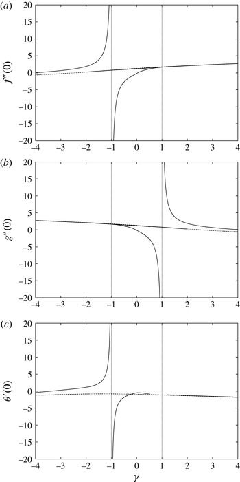
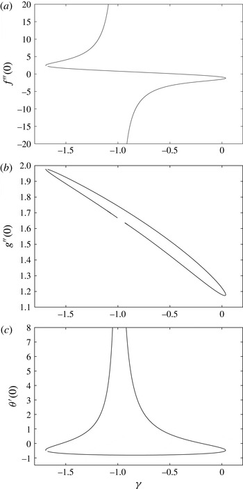
Forced convection: plots of (a)
 $f^{\prime \prime }(0)$
, (b)
 $g^{\prime \prime }(0)$
and (c)
 $\unicode[STIX]{x1D703}^{\prime }(0)$
against
 $\unicode[STIX]{x1D6FE}$
obtained from the numerical solution of (2.8)–(2.11). The previous results given by Weidman (Reference Weidman2012) for the flow problem and the corresponding forced convection solution are shown by the broken lines.




We can now exploit the symmetry given in Weidman (Reference Weidman2012) of
 $\unicode[STIX]{x1D6FE}\rightarrow -\unicode[STIX]{x1D6FE}$
,
 $f\rightarrow g$
and
 $g\rightarrow f$
to extend this analysis to show that there is also a singularity as
 $\unicode[STIX]{x1D6FE}\rightarrow 1$
with
 $$\begin{eqnarray}\displaystyle f^{\prime \prime }(0)\rightarrow 1.66588+\cdots \,,\quad g^{\prime \prime }(0)\sim -1.78068(1-\unicode[STIX]{x1D6FE})^{-1}+\cdots \quad \text{as }\unicode[STIX]{x1D6FE}\rightarrow 1.\qquad & & \displaystyle\end{eqnarray}$$
We can use expressions (3.10) and (3.11) to generate further numerical solutions starting the integrations close to
 $\unicode[STIX]{x1D6FE}=-1$
and to
 $\unicode[STIX]{x1D6FE}=1$
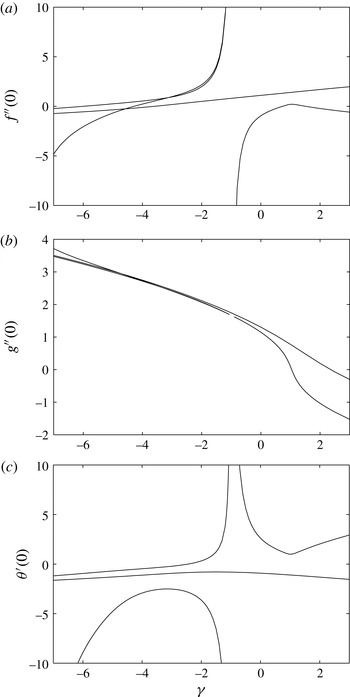
. These are shown in figure 1(a,b) to compare with the previous results given by Weidman (Reference Weidman2012) (shown by broken lines). The singular nature of
 $f^{\prime \prime }(0)$
as
 $\unicode[STIX]{x1D6FE}\rightarrow -1$
and of
 $g^{\prime \prime }(0)$
as
 $\unicode[STIX]{x1D6FE}\rightarrow 1$
is clearly seen in figure 1. For large
 $|\unicode[STIX]{x1D6FE}|$
the solutions follow closely the solution given by Weidman. The results for the corresponding heat transfer problem are shown in figure 1(c) where the full lines are these additional solutions and the broken lines are the results for the heat transfer derived from the solutions given previously by Weidman for the flow problem. We see that
 $\unicode[STIX]{x1D703}^{\prime }(0)$
becomes singular as
 $\unicode[STIX]{x1D6FE}\rightarrow -1$
arising from the singular nature of the solution for
 $f(\unicode[STIX]{x1D702})$
. However, the singularity in
 $g(\unicode[STIX]{x1D702})$
as
 $\unicode[STIX]{x1D6FE}\rightarrow 1$
does not seem to affect the solution for
 $\unicode[STIX]{x1D703}(\unicode[STIX]{x1D702})$
, with the values of
 $\unicode[STIX]{x1D703}^{\prime }(0)$
appearing to progress smoothly through this value of
 $\unicode[STIX]{x1D6FE}$
. We note that Weidman (Reference Weidman2012) mentioned the possibility of further solutions to the forced convection problem, perhaps with a velocity overshoot, but did not plot them.
3.2 Numerical results
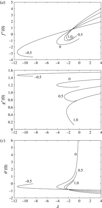
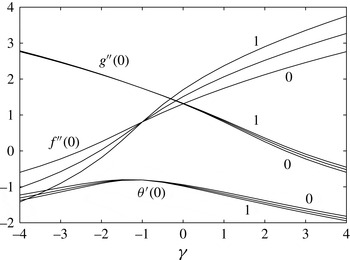
In figure 2 we plot
 $f^{\prime \prime }(0)$
,
 $g^{\prime \prime }(0)$
and
 $\unicode[STIX]{x1D703}^{\prime }(0)$
against
 $\unicode[STIX]{x1D706}$
for representative values of
 $\unicode[STIX]{x1D6FE}>-1$
, noting for
 $\unicode[STIX]{x1D6FE}=-1$
that the solution is independent of
 $\unicode[STIX]{x1D706}$
. A significant feature of these results is the existence of a critical value
 $\unicode[STIX]{x1D706}_{c}$
of
 $\unicode[STIX]{x1D706}$
with the saddle-node bifurcation at
 $\unicode[STIX]{x1D706}=\unicode[STIX]{x1D706}_{c}$
producing two solution branches in
 $\unicode[STIX]{x1D706}\geqslant \unicode[STIX]{x1D706}_{c}$
. These critical values depend on
 $\unicode[STIX]{x1D6FE}$
with
 $|\unicode[STIX]{x1D706}_{c}|$
increasing noticeably as
 $\unicode[STIX]{x1D6FE}$
approaches
 $-1$
. The upper solution branch, as seen in figure 2(a), continues to large positive
 $\unicode[STIX]{x1D706}$
with the values of
 $f^{\prime \prime }(0)$
and
 $g^{\prime \prime }(0)$
increasing and
 $\unicode[STIX]{x1D703}^{\prime }(0)$
decreasing. The lower branch terminates at a finite value of
 $\unicode[STIX]{x1D706}$
; our numerical results suggest that this might be as
 $\unicode[STIX]{x1D706}\rightarrow 0$
from below with
 $\unicode[STIX]{x1D703}^{\prime }(0)$
becoming increasingly larger. Figure 2 leads us to consider the critical points in more detail.
3.2.1 Critical values
We can calculate the critical values numerically following the approach given in Merkin & Mahmood (Reference Merkin and Mahmood1989) and Merkin & Pop (Reference Merkin and Pop2010), for example. In this we make a linear perturbation to (2.8)–(2.11). This results in a linear eigenvalue homogeneous problem for the critical value
 $\unicode[STIX]{x1D706}_{c}$
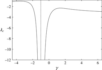
. In figure 3 we plot the values of
 $\unicode[STIX]{x1D706}_{c}$
against
 $\unicode[STIX]{x1D6FE}$
obtained by this method. These results agree with the values of
 $\unicode[STIX]{x1D706}_{c}$
seen in figure 2. We see that there are two sections to the graph, one for
 $\unicode[STIX]{x1D6FE}>-1$
and the other for
 $\unicode[STIX]{x1D6FE}<-1$
, with
 $\unicode[STIX]{x1D706}_{c}<0$
throughout. The values of
 $|\unicode[STIX]{x1D706}_{c}|$
increase rapidly as
 $\unicode[STIX]{x1D6FE}\rightarrow -1$
in both sections, as might be expected from the singular nature of the forced convection solution at
 $\unicode[STIX]{x1D6FE}=-1$
discussed above. Our numerical results suggest that
 $\unicode[STIX]{x1D706}_{c}$
is approaching constant values as
 $\unicode[STIX]{x1D6FE}\rightarrow \infty$
and as
 $\unicode[STIX]{x1D6FE}\rightarrow -\infty$
. A more detailed discussion of the solution for large
 $|\unicode[STIX]{x1D6FE}|$
is given below.
Critical values: a plot of
 $\unicode[STIX]{x1D706}_{c}$
against
 $\unicode[STIX]{x1D6FE}$
.

The existence of critical points for
 $\unicode[STIX]{x1D6FE}<-1$
seen in figure 3 leads us to examine the case when
 $\unicode[STIX]{x1D6FE}<-1$
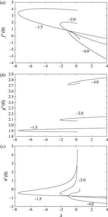
in more detail with plots of
 $f^{\prime \prime }(0)$
,
 $g^{\prime \prime }(0)$
and
 $\unicode[STIX]{x1D703}^{\prime }(0)$
against
 $\unicode[STIX]{x1D706}$
shown in figure 4. We see a similar picture to that seen in figure 2, namely that there is a critical value
 $\unicode[STIX]{x1D706}_{c}$
still dependent on
 $\unicode[STIX]{x1D6FE}$
and which also has
 $|\unicode[STIX]{x1D706}_{c}|$
increasing as
 $\unicode[STIX]{x1D6FE}\rightarrow -1$
from below in agreement with figure 3. The upper branch continues to large
 $\unicode[STIX]{x1D706}$
and the lower branch terminates as
 $\unicode[STIX]{x1D706}\rightarrow 0$
. The only difference from figure 2 is that the values of
 $f^{\prime \prime }(0)$
are negative for large positive
 $\unicode[STIX]{x1D706}$
.




We now consider how the solution varies with
 $\unicode[STIX]{x1D6FE}$
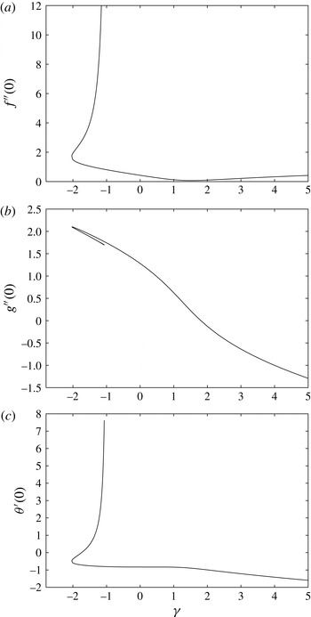
, and in figure 5 we plot
 $f^{\prime \prime }(0)$
,
 $g^{\prime \prime }(0)$
and
 $\unicode[STIX]{x1D703}^{\prime }(0)$
against
 $\unicode[STIX]{x1D6FE}$
for values of
 $\unicode[STIX]{x1D706}$
representative of aiding flow,
 $\unicode[STIX]{x1D706}>0$
; the forced convection,
 $\unicode[STIX]{x1D706}=0$
, is shown for comparison. We see that, in all cases, the solution proceeds to both large positive and large negative values of
 $\unicode[STIX]{x1D6FE}$
. For the values of
 $\unicode[STIX]{x1D706}$
taken, the values of
 $g^{\prime \prime }(0)$
vary only slightly from their forced convection values whereas there is a somewhat greater variation in
 $f^{\prime \prime }(0)$
and
 $\unicode[STIX]{x1D703}^{\prime }(0)$
. When
 $\unicode[STIX]{x1D6FE}=-1$
the problem becomes essentially forced convection, independent of
 $\unicode[STIX]{x1D706}$
, with all the curves passing through the same values of
 $f^{\prime \prime }(0)=0.80676$
,
 $g^{\prime \prime }(0)=1.74314$
and
 $\unicode[STIX]{x1D703}^{\prime }(0)=-0.80676$
, noting, for
 $Pr=1.0$
, that
 $\unicode[STIX]{x1D703}=1-f^{\prime }$
when
 $\unicode[STIX]{x1D6FE}=-1$
.


We next consider opposing flow,
 $\unicode[STIX]{x1D706}<0$
, starting with plots of
 $f^{\prime \prime }(0)$
,
 $g^{\prime \prime }(0)$
and
 $\unicode[STIX]{x1D703}^{\prime }(0)$
against
 $\unicode[STIX]{x1D6FE}$
for
 $\unicode[STIX]{x1D706}=-0.5$
in figure 6. Here we see that there are four disjoint solution sections. One section proceeds to both large positive and large negative values of
 $\unicode[STIX]{x1D6FE}$
(as seen in aiding flow); the other solution sections becoming singular as
 $\unicode[STIX]{x1D6FE}\rightarrow -1$
. Similar results to those shown in figure 6 were found for
 $\unicode[STIX]{x1D706}=-1.0$
. These results agree with the behaviour seen in figure 3 that there appear to be no critical values for this value of
 $\unicode[STIX]{x1D706}$
. However, for larger negative values of
 $\unicode[STIX]{x1D706}$
, figure 6 indicates the possibility of one, two or three critical points, and this is what we next consider by taking representative values of
 $\unicode[STIX]{x1D706}$
for each case.
In figure 7 we plot
 $f^{\prime \prime }(0)$
,
 $g^{\prime \prime }(0)$
and
 $\unicode[STIX]{x1D703}^{\prime }(0)$
against
 $\unicode[STIX]{x1D6FE}$
for
 $\unicode[STIX]{x1D706}=-2.0$
. Here there is just one critical point at
 $\unicode[STIX]{x1D6FE}\simeq -2.040$
giving rise to two solution branches. The lower branch, as seen in figure 7(a), proceeds to large positive
 $\unicode[STIX]{x1D6FE}$
and the upper branch becomes singular as
 $\unicode[STIX]{x1D6FE}\rightarrow -1$
with both
 $f^{\prime \prime }(0)$
and
 $\unicode[STIX]{x1D703}^{\prime }(0)$
becoming large though
 $g^{\prime \prime }(0)$
remains finite. For
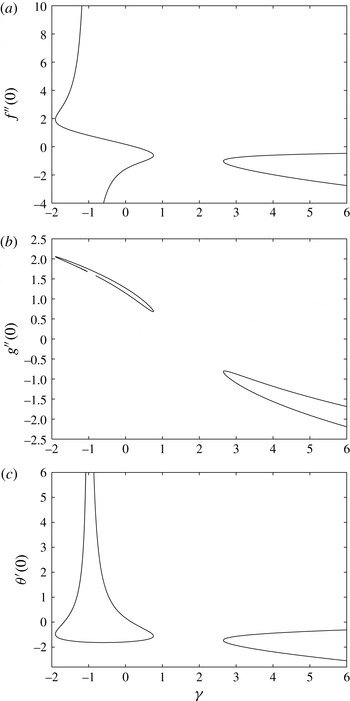
 $\unicode[STIX]{x1D706}=-2.5$
there are three critical points at
 $\unicode[STIX]{x1D6FE}\simeq -1.880,0.749$
and
 $2.649$
, which we can see in figure 8. Here there are two solution sections, one in
 $\unicode[STIX]{x1D6FE}<1$
and the other in
 $\unicode[STIX]{x1D6FE}>1$
. The solution section in
 $\unicode[STIX]{x1D6FE}<1$
has three solution branches arising from the two saddle-node bifurcations in this region with the upper and lower branches becoming singular as
 $\unicode[STIX]{x1D6FE}\rightarrow -1$
. The solution in
 $\unicode[STIX]{x1D6FE}>1$
has two branches arising from the critical point at
 $\unicode[STIX]{x1D6FE}=2.649$
, with both branches proceeding to large
 $\unicode[STIX]{x1D6FE}$
. For
 $\unicode[STIX]{x1D706}=-4.0$
there are two critical points at
 $\unicode[STIX]{x1D6FE}\simeq -1.696$
and
 $0.038$
with the results being plotted in figure 9. Here there are three branches, the middle branch connecting the two critical points, and the upper and lower branches becoming singular as
 $\unicode[STIX]{x1D6FE}\rightarrow -1$
.


The plots shown in figures 2 and 4 indicate there is a limiting form as
 $\unicode[STIX]{x1D706}\rightarrow \infty$
, which is what we now consider.
3.3 Free convection limit,
$\unicode[STIX]{x1D706}$
large

We assume that
 $\unicode[STIX]{x1D6FE}\neq -1$
and to obtain a solution valid for
 $\unicode[STIX]{x1D706}\gg 1$
we put, following Revnic et al. (Reference Revnic, Grosan, Merkin and Pop2009), for example,
 $$\begin{eqnarray}\displaystyle f=\unicode[STIX]{x1D706}^{1/4}\unicode[STIX]{x1D719},\quad g=\unicode[STIX]{x1D706}^{1/4}h,\quad \unicode[STIX]{x1D709}=\unicode[STIX]{x1D706}^{1/4}\unicode[STIX]{x1D702}. & & \displaystyle\end{eqnarray}$$
Equations (2.8)–(2.11) then become
 $$\begin{eqnarray}\displaystyle & \displaystyle \unicode[STIX]{x1D719}^{\prime \prime \prime }+(1+\unicode[STIX]{x1D6FE})(\unicode[STIX]{x1D719}\unicode[STIX]{x1D719}^{\prime \prime }-\unicode[STIX]{x1D719}^{\prime 2})+(1-\unicode[STIX]{x1D6FE})h\unicode[STIX]{x1D719}^{\prime \prime }+(1+\unicode[STIX]{x1D6FE})\unicode[STIX]{x1D706}^{-1}+(1+\unicode[STIX]{x1D6FE})\unicode[STIX]{x1D703}=0, & \displaystyle\end{eqnarray}$$
 $$\begin{eqnarray}\displaystyle & \displaystyle h^{\prime \prime \prime }+(1-\unicode[STIX]{x1D6FE})(hh^{\prime \prime }-h^{\prime 2})+(1+\unicode[STIX]{x1D6FE})\unicode[STIX]{x1D719}h^{\prime \prime }+(1-\unicode[STIX]{x1D6FE})\unicode[STIX]{x1D706}^{-1}=0, & \displaystyle\end{eqnarray}$$
 $$\begin{eqnarray}\displaystyle & \displaystyle \frac{1}{Pr}\unicode[STIX]{x1D703}^{\prime \prime }+(1+\unicode[STIX]{x1D6FE})(\unicode[STIX]{x1D719}\unicode[STIX]{x1D703}^{\prime }-\unicode[STIX]{x1D719}^{\prime }\unicode[STIX]{x1D703})+(1-\unicode[STIX]{x1D6FE})h\unicode[STIX]{x1D703}^{\prime }=0, & \displaystyle\end{eqnarray}$$
subject to the boundary conditions
 $$\begin{eqnarray}\displaystyle \left.\begin{array}{@{}c@{}}\displaystyle \unicode[STIX]{x1D719}(0)=\unicode[STIX]{x1D719}^{\prime }(0)=h(0)=h^{\prime }(0)=0,\quad \unicode[STIX]{x1D703}(0)=1,\\ \displaystyle \unicode[STIX]{x1D719}^{\prime }\rightarrow \unicode[STIX]{x1D706}^{-1/2},~h^{\prime }\rightarrow \unicode[STIX]{x1D706}^{-1/2},~\unicode[STIX]{x1D703}\rightarrow 0\text{ as }\unicode[STIX]{x1D709}\rightarrow \infty ,\end{array}\right\} & & \displaystyle\end{eqnarray}$$
and where primes now denote differentiation with respect to
 $\unicode[STIX]{x1D709}$
.
An expansion in powers of
 $\unicode[STIX]{x1D706}^{-1/2}$
is suggested by boundary conditions (3.16). However, if we apply this directly in (3.14) we see that the leading-order term in
 $h$
is identically zero. This then suggests a solution by expanding
 $$\begin{eqnarray}\displaystyle \unicode[STIX]{x1D719}=\unicode[STIX]{x1D719}_{0}+\unicode[STIX]{x1D706}^{-1/2}\unicode[STIX]{x1D719}_{1}+\cdots \,,\quad h=\unicode[STIX]{x1D706}^{-1/2}h_{0}+\unicode[STIX]{x1D706}^{-1}h_{1}+\cdots \,,\quad \unicode[STIX]{x1D703}=\unicode[STIX]{x1D703}_{0}+\unicode[STIX]{x1D706}^{-1/2}\unicode[STIX]{x1D703}_{1}+\cdots \,. & & \displaystyle \nonumber\\ \displaystyle & & \displaystyle\end{eqnarray}$$
We obtain, at leading order,
 $$\begin{eqnarray}\displaystyle & \displaystyle \unicode[STIX]{x1D719}_{0}^{\prime \prime \prime }+(1+\unicode[STIX]{x1D6FE})(\unicode[STIX]{x1D719}_{0}\unicode[STIX]{x1D719}_{0}^{\prime \prime }-\unicode[STIX]{x1D719}_{0}^{\prime 2})+(1+\unicode[STIX]{x1D6FE})\unicode[STIX]{x1D703}_{0}=0, & \displaystyle\end{eqnarray}$$
 $$\begin{eqnarray}\displaystyle & \displaystyle h_{0}^{\prime \prime \prime }+(1+\unicode[STIX]{x1D6FE})\unicode[STIX]{x1D719}_{0}h_{0}^{\prime \prime }=0, & \displaystyle\end{eqnarray}$$
 $$\begin{eqnarray}\displaystyle & \displaystyle \frac{1}{Pr}\unicode[STIX]{x1D703}_{0}^{\prime \prime }+(1+\unicode[STIX]{x1D6FE})(\unicode[STIX]{x1D719}_{0}\unicode[STIX]{x1D703}_{0}^{\prime }-\unicode[STIX]{x1D719}_{0}^{\prime }\unicode[STIX]{x1D703}_{0})=0, & \displaystyle\end{eqnarray}$$
subject to the boundary conditions
 $$\begin{eqnarray}\displaystyle \left.\begin{array}{@{}c@{}}\displaystyle \unicode[STIX]{x1D719}_{0}(0)=\unicode[STIX]{x1D719}_{0}^{\prime }(0)=h_{0}(0)=h_{0}^{\prime }(0)=0,\quad \unicode[STIX]{x1D703}_{0}(0)=1,\\ \displaystyle \unicode[STIX]{x1D719}_{0}^{\prime }\rightarrow 0,~h_{0}^{\prime }\rightarrow 1,~\unicode[STIX]{x1D703}_{0}\rightarrow 0\text{ as }\unicode[STIX]{x1D709}\rightarrow \infty .\end{array}\right\} & & \displaystyle\end{eqnarray}$$
We can remove
 $\unicode[STIX]{x1D6FE}$
from (3.18)–(3.20) by writing
 $$\begin{eqnarray}\displaystyle \unicode[STIX]{x1D719}_{0}=(1+\unicode[STIX]{x1D6FE})^{-1/2}\overline{\unicode[STIX]{x1D719}}_{0},\quad \overline{\unicode[STIX]{x1D709}}=(1+\unicode[STIX]{x1D6FE})^{1/2}\unicode[STIX]{x1D709},\quad \text{if }\unicode[STIX]{x1D6FE}>-1 & & \displaystyle\end{eqnarray}$$
and
 $$\begin{eqnarray}\displaystyle \unicode[STIX]{x1D719}_{0}=-(-(1+\unicode[STIX]{x1D6FE}))^{-1/2}\overline{\unicode[STIX]{x1D719}}_{0},\quad \overline{\unicode[STIX]{x1D709}}=(-(1+\unicode[STIX]{x1D6FE}))^{1/2}\unicode[STIX]{x1D709},\quad \text{if }\unicode[STIX]{x1D6FE}<-1 & & \displaystyle\end{eqnarray}$$
to obtain
 $$\begin{eqnarray}\displaystyle & \displaystyle \overline{\unicode[STIX]{x1D719}}_{0}^{\prime \prime \prime }+(\overline{\unicode[STIX]{x1D719}}_{0}\overline{\unicode[STIX]{x1D719}}_{0}^{\prime \prime }-\overline{\unicode[STIX]{x1D719}}_{0}^{\prime 2})+\unicode[STIX]{x1D703}_{0}=0, & \displaystyle\end{eqnarray}$$
 $$\begin{eqnarray}\displaystyle & \displaystyle h_{0}^{\prime \prime \prime }+\overline{\unicode[STIX]{x1D719}}_{0}h_{0}^{\prime \prime }=0, & \displaystyle\end{eqnarray}$$
 $$\begin{eqnarray}\displaystyle & \displaystyle \frac{1}{Pr}\unicode[STIX]{x1D703}_{0}^{\prime \prime }+(\overline{\unicode[STIX]{x1D719}}_{0}\unicode[STIX]{x1D703}_{0}^{\prime }-\overline{\unicode[STIX]{x1D719}}_{0}^{\prime }\unicode[STIX]{x1D703}_{0})=0, & \displaystyle\end{eqnarray}$$
still subject to boundary conditions (3.21). A numerical integration of (3.24)–(3.26) gives, for
 $Pr=1.0$
,
 $\overline{\unicode[STIX]{x1D719}}_{0}^{\prime \prime }(0)=0.73950,~h_{0}^{\prime \prime }(0)=0.39270,~\unicode[STIX]{x1D703}_{0}^{\prime }(0)=-0.59509$
so that, when
 $\unicode[STIX]{x1D6FE}>1$
,
 $$\begin{eqnarray}\displaystyle \left.\begin{array}{@{}c@{}}\displaystyle f^{\prime \prime }(0)\sim 0.73950(1+\unicode[STIX]{x1D6FE})^{1/2}\unicode[STIX]{x1D706}^{3/4}+\cdots \,,\quad g^{\prime \prime }(0)\sim 0.39270(1+\unicode[STIX]{x1D6FE})\unicode[STIX]{x1D706}^{1/4}+\cdots \,,\\ \displaystyle \unicode[STIX]{x1D703}^{\prime }(0)\sim -0.59509(1+\unicode[STIX]{x1D6FE})^{1/2}\unicode[STIX]{x1D706}^{1/4}+\cdots \,,\end{array}\right\}\qquad & & \displaystyle\end{eqnarray}$$
or, when
 $\unicode[STIX]{x1D6FE}<-1$
,
 $$\begin{eqnarray}\displaystyle \left.\begin{array}{@{}c@{}}\displaystyle f^{\prime \prime }(0)\sim -0.73950(-(1+\unicode[STIX]{x1D6FE}))^{1/2}\unicode[STIX]{x1D706}^{3/4}+\cdots \,,\quad g^{\prime \prime }(0)\sim 0.39270|(1+\unicode[STIX]{x1D6FE})|\unicode[STIX]{x1D706}^{1/4}+\cdots \,,\\ \displaystyle \unicode[STIX]{x1D703}^{\prime }(0)\sim -0.59509(-(1+\unicode[STIX]{x1D6FE}))^{1/2}\unicode[STIX]{x1D706}^{1/4}+\cdots \,,\end{array}\right\}\hspace{-16.79993pt} & & \displaystyle \nonumber\\ \displaystyle & & \displaystyle\end{eqnarray}$$
as
 $\unicode[STIX]{x1D706}\rightarrow \infty$
. These results are consistent with the values seen in figures 2 and 4.
3.4 Large
$\unicode[STIX]{x1D6FE}$

The nature of the solution for
 $\unicode[STIX]{x1D6FE}$
was treated in Weidman (Reference Weidman2012) for forced convection and we can extend this analysis to the present case. Following Weidman, we apply the transformation
 $f=\unicode[STIX]{x1D6FE}^{-1/2}F,~g=\unicode[STIX]{x1D6FE}^{-1/2}G,~\unicode[STIX]{x1D701}=\unicode[STIX]{x1D6FE}^{1/2}\unicode[STIX]{x1D702}$
, and we obtain
 $$\begin{eqnarray}\displaystyle & \displaystyle F^{\prime \prime \prime }+(1+\unicode[STIX]{x1D6FE}^{-1})(FF^{\prime \prime }+1-F^{\prime 2})-(1-\unicode[STIX]{x1D6FE}^{-1})GF^{\prime \prime }+(1+\unicode[STIX]{x1D6FE}^{-1})\unicode[STIX]{x1D706}\unicode[STIX]{x1D703}=0, & \displaystyle\end{eqnarray}$$
 $$\begin{eqnarray}\displaystyle & \displaystyle G^{\prime \prime \prime }-(1-\unicode[STIX]{x1D6FE}^{-1})(GG^{\prime \prime }-1+G^{\prime 2})+(1+\unicode[STIX]{x1D6FE}^{-1})FG^{\prime \prime }=0, & \displaystyle\end{eqnarray}$$
 $$\begin{eqnarray}\displaystyle & \displaystyle \frac{1}{Pr}\unicode[STIX]{x1D703}^{\prime \prime }+(1+\unicode[STIX]{x1D6FE}^{-1})(F\unicode[STIX]{x1D703}^{\prime }-F^{\prime }\unicode[STIX]{x1D703})-(1-\unicode[STIX]{x1D6FE}^{-1})G\unicode[STIX]{x1D703}^{\prime }=0, & \displaystyle\end{eqnarray}$$
still subject to boundary conditions (2.11) and where primes now denote differentiation with respect to
 $\unicode[STIX]{x1D701}$
.
We obtain, at leading order,
 $$\begin{eqnarray}\displaystyle F^{\prime \prime \prime }+FF^{\prime \prime }+1-F^{\prime 2}-GF^{\prime \prime }+\unicode[STIX]{x1D706}\unicode[STIX]{x1D703}=0,\quad G^{\prime \prime \prime }-GG^{\prime \prime }-1+G^{\prime 2}+FG^{\prime \prime }=0\qquad & & \displaystyle\end{eqnarray}$$
together with
 $$\begin{eqnarray}\displaystyle \frac{1}{Pr}\unicode[STIX]{x1D703}^{\prime \prime }+F\unicode[STIX]{x1D703}^{\prime }-F^{\prime }\unicode[STIX]{x1D703}-G\unicode[STIX]{x1D703}^{\prime }=0, & & \displaystyle\end{eqnarray}$$
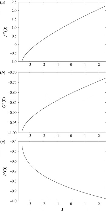
still subject to the boundary conditions given in (2.11). We plot the values of
 $F^{\prime \prime }(0),~G^{\prime \prime }(0)$
and
 $\unicode[STIX]{x1D703}^{\prime }(0)$
obtained from the numerical solution of (3.32) and (3.33) in figure 10.


For
 $\unicode[STIX]{x1D706}$
large we can apply transformation (3.12) in (3.32) and (3.33) to obtain (3.24)–(3.26) at leading order, giving, in the limit of large
 $\unicode[STIX]{x1D6FE}$
and
 $\unicode[STIX]{x1D706}$
,
 $$\begin{eqnarray}\displaystyle \left.\begin{array}{@{}c@{}}\displaystyle f^{\prime \prime }(0)\sim 0.7395\unicode[STIX]{x1D706}^{3/4}\unicode[STIX]{x1D6FE}^{1/2}+\cdots \,,\quad g^{\prime \prime }(0)\sim 0.3927\unicode[STIX]{x1D706}^{1/4}\unicode[STIX]{x1D6FE}^{1/2}+\cdots \,,\\ \displaystyle \unicode[STIX]{x1D703}^{\prime }(0)\sim -0.5951\unicode[STIX]{x1D706}^{1/4}\unicode[STIX]{x1D6FE}^{1/2}+\cdots \end{array}\right\} & & \displaystyle\end{eqnarray}$$
for
 $Pr=1.0$
, consistent with expressions (3.27) in the large-
 $\unicode[STIX]{x1D6FE}$
limit.
We have seen in figures 5 and 6 that the solution can continue to large negative values of
 $\unicode[STIX]{x1D6FE}$
. We can adapt our analysis to this case by writing
 $|\unicode[STIX]{x1D6FE}|$
for
 $\unicode[STIX]{x1D6FE}$
in the transformation and then replacing
 $F$
by
 $-F$
and
 $G$
by
 $-G$
in (3.32) and (3.33).
4 Conclusions
We have extended the results given previously by Weidman (Reference Weidman2012) for the non-axisymmetric Homann stagnation-point flow to include mixed convection effects. Two uniform shear flows are superimposed onto the Homann stagnation-point flow; hence the resulting similarity equations (2.8)–(2.10) subject to boundary conditions (2.11) were seen to involve the mixed convection or buoyancy parameter
 $\unicode[STIX]{x1D706}$
as well as the shear-to-strain-rate ratio
 $\unicode[STIX]{x1D6FE}$
, measuring the strength of the outer (inviscid) flow. The momentum equations (2.8)–(2.10) are coupled, hence need to be solved simultaneously. The parameter
 $\unicode[STIX]{x1D706}$
represents the strength of the natural convection relative to that of forced convection. The limiting values of
 $\unicode[STIX]{x1D706}=0$
and
 $\unicode[STIX]{x1D706}\rightarrow \infty$
correspond respectively to the forced and natural (free) convection limits. The study of mixed convection finds application in many industrial and technical processes where there are temperature differences between the bounding surface and ambient conditions, thereby modifying both the flow and temperature fields. Throughout we took the Prandtl number
 $Pr=1$
, close to the value of
 $Pr\simeq 0.7$
for air.
It was pointed out by Weidman (Reference Weidman2012) that multiple solution branches are expected to exist in this new family of Homann stagnation-point flows with the introduction of the parameter
 $\unicode[STIX]{x1D6FE}$
and hence we started by considering the forced convection,
 $\unicode[STIX]{x1D706}=0$
, solution, finding additional solutions to those presented previously by Weidman (see figure 1). These extra solutions derive from singularities in the solution that can arise as
 $\unicode[STIX]{x1D6FE}\rightarrow -1$
(
 $b=-a$
) and as
 $\unicode[STIX]{x1D6FE}\rightarrow 1$
(
 $b=a$
); see expressions (3.10) and (3.11).
We then examined how the solution varied with
 $\unicode[STIX]{x1D706}$
for representative values of
 $\unicode[STIX]{x1D6FE}>-1$
(figure 2). The main features found here are that the solution proceeded to large positive
 $\unicode[STIX]{x1D706}$
and, perhaps more significantly, that there are critical values
 $\unicode[STIX]{x1D706}_{c}$
, dependent on
 $\unicode[STIX]{x1D6FE}$
, limiting the range of solutions to
 $\unicode[STIX]{x1D706}\geqslant \unicode[STIX]{x1D706}_{c}$
. This led us to treat these critical values in more detail (figure 3), showing also the existence of critical values for
 $\unicode[STIX]{x1D6FE}<-1$
, which we examined in figure 4. Our calculations of these critical points became singular as
 $\unicode[STIX]{x1D6FE}\rightarrow -1$
as, perhaps, could be expected from the forced convection solution and shown in figure 1.
The existence of buoyancy-induced convection changed the behaviour of these flows significantly. We looked at how the solution varied with
 $\unicode[STIX]{x1D6FE}$
for representative values of
 $\unicode[STIX]{x1D706}$
starting with aiding flow
 $\unicode[STIX]{x1D706}>0$
(figure 5). Our results indicated that the solution continued to large positive and large negative values of
 $\unicode[STIX]{x1D6FE}$
. We then considered opposing flow,
 $\unicode[STIX]{x1D706}<0$
(figures 6–9), motivated by our discussion of the critical values with there being the possibility, for
 $\unicode[STIX]{x1D706}<-1.0$
, of having one, two or three critical points. In each case we saw a singularity in the solution as
 $\unicode[STIX]{x1D6FE}\rightarrow -1$
. However, the singularity seen as
 $\unicode[STIX]{x1D6FE}\rightarrow 1$
for forced convection did not appear to be reflected in these solutions. This might be accounted for by the fact that, since the temperature
 $\unicode[STIX]{x1D703}(\unicode[STIX]{x1D702})$
field plays a more significant role in mixed convection for the shear flow
 $f(\unicode[STIX]{x1D702})$
and as seen in figure 1(c), the temperature field appears smooth as
 $\unicode[STIX]{x1D6FE}$
passes through
 $\unicode[STIX]{x1D6FE}=1$
.
An asymptotic solution for the free convection limit,
 $\unicode[STIX]{x1D706}\rightarrow \infty$
, was then derived, reducing the problem to one independent of
 $\unicode[STIX]{x1D6FE}$
, equations (3.24)–(3.26) leading to expressions (3.27) and (3.28). The scalings (3.12) for this limit were chosen to balance the viscous term, the convective terms and the buoyancy term in (2.8), with the outer flow appearing at higher order. We discussed the large positive
 $\unicode[STIX]{x1D6FE}$
solution, being an extension of that derived by Weidman (Reference Weidman2012) to the mixed convection case, indicating how this could be modified to large negative values of
 $\unicode[STIX]{x1D6FE}$
. Finally we comment on the temporal stability of the solutions arising from the time-dependent version of the present case. The saddle-node bifurcation, a real eigenvalue passing through zero, at the critical points will lead to a change in the stability of the solution. Which branch is stable when there are dual and multiple solutions and how this change in local stability affects the behaviour of the full time-dependent problem is beyond the scope of the present paper, though well worth further study.
The basic fluid flow problem considered here is described fully by Weidman (Reference Weidman2012). Having the bounding surface heated, as here at a temperature above that of the ambient fluid, can have a significant influence on this basic flow. Analysis indicates that the parameter that characterizes mixed convection is
 $\unicode[STIX]{x1D706}=Gr/Re^{n}$
, where the Grashof number
 $Gr$
and the Reynolds number
 $Re$
represent the strength of the natural convection and forced flow effects, respectively. The exponent
 $n$
depends on the geometry, the thermal boundary condition, the type of fluid, etc. In the present case
 $n=2$
(Gebhart et al.
Reference Gebhart, Jaluria, Mahajan and Sammakia1988). When the buoyancy forces generated by the wall heating act in the same direction as the external forcing, here having
 $\unicode[STIX]{x1D706}>0$
, this can lead to a much enhanced flow achieving flow velocities much greater than would be seen otherwise. Alternatively, when the buoyancy forces act in the opposite direction to the external forcing,
 $\unicode[STIX]{x1D706}<0$
, these can limit the existence of an attached flow, as here through critical values
 $\unicode[STIX]{x1D706}_{c}$
of
 $\unicode[STIX]{x1D706}$
and, more generally, lead to instability and flow separation. A detailed knowledge of how the wall heating affects the flow is an essential prerequisite to understanding these features.