


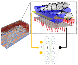



1. Introduction
Turbulent flows are ubiquitous in our daily life and determine the performances and the energy efficiencies of various thermo-fluids devices (Brunton & Noack Reference Brunton and Noack2015). In most engineering flows, turbulence is bounded by a solid surface, and their interaction plays a crucial role in generation and maintenance of near-wall turbulence, and associated momentum and heat transport between fluid and solid. Even over simple geometries such as a smooth flat wall, however, turbulence exhibits complex behaviour due to its nonlinear and multiscale nature, so that prediction and control of turbulent flow remain challenging.
In this study, we consider the control of a fully developed turbulent channel flow, which is one of the canonical flow configurations. Since near-wall turbulence is responsible for the increase in wall skin friction, a tremendous amount of effort has been devoted to reducing the skin friction drag. In general, flow control strategies can be categorized into passive and active schemes (Gad-el Hak Reference Gad-el Hak1996). The passive scheme does not require power input for control, and its typical example is a riblet surface (Dean & Bhushan Reference Dean and Bhushan2010). In contrast, the active scheme requires additional power input for control, and it can be further classified into predetermined and feedback controls. The former applies a control input with a predetermined spatio-temporal distribution regardless of an instantaneous flow state. This makes a control system simple since no sensing of a flow field is required. Despite its simplicity, it is known that the predetermined control achieves relatively high drag reduction rates, and various control modes, such as spanwise wall oscillation (Jung, Mangiavacchi & Akhavan Reference Jung, Mangiavacchi and Akhavan1992; Quadrio & Ricco Reference Quadrio and Ricco2004), streamwise travelling wave of wall blowing and suction (Min et al. Reference Min, Kang, Speyer and Kim2006; Lieu, Marref & Jovanović Reference Lieu, Marref and Jovanović2010; Mamori, Iwamoto & Murata Reference Mamori, Iwamoto and Murata2014), and uniform wall blowing (Sumitani & Kasagi Reference Sumitani and Kasagi1995; Kametani & Fukagata Reference Kametani and Fukagata2011), have been proposed.
In contrast, the feedback control determines a control input based on a sensor signal obtained from an instantaneous flow field, therefore it enables a more flexible control. Meanwhile, due to the large degrees of freedom of the flow state and also the control input, optimizing a feedback control law is quite challenging. Therefore, existing control strategies have often been developed based on researchers’ physical insights. A typical example of a feedback control is the so-called opposition control (Choi, Moin & Kim Reference Choi, Moin and Kim1994; Hammond, Bewley & Moin Reference Hammond, Bewley and Moin1998; Chung & Talha Reference Chung and Talha2011), where local wall blowing and suction is applied so as to cancel the wall-normal velocity fluctuation at a certain height from the wall. The sensing plane is called a detection plane, and its optimal height has been reported as  $y^+=15$ in a wall unit (Hammond et al. Reference Hammond, Bewley and Moin1998). The relationship between the wall-normal velocity on the detection plane and the control input has been assumed commonly to be linear a priori, and its optimal weight coefficient was found to be approximately unity (Choi et al. Reference Choi, Moin and Kim1994; Chung & Talha Reference Chung and Talha2011). It should be noted that optimization of these parameters in the control algorithm has mostly been done through trial and error, and such an approach is quite inefficient even for a simple control algorithm where the relationship between the sensor signal and the control input is assumed to be linear.
There also exists another approach to develop efficient feedback control laws. Optimal control theory is a powerful tool to optimize a control input with large degrees of freedom by explicitly leveraging mathematical models of a flow system such as Navier–Stokes equations and mass conservation. Specifically, the spatio-temporal distribution of a control input is determined so as to minimize a prescribed cost functional. The cost functional can be defined within a certain time horizon, so that the future flow dynamics is taken into consideration in the optimization procedures. Optimal control theory was applied successfully to a low-Reynolds-number turbulent channel flow by Bewley, Moin & Temam (Reference Bewley, Moin and Temam2001), and it was demonstrated that the flow can be relaminarized. One of the major drawbacks in optimal control theory is that it requires expensive iterations of forward and adjoint simulations within the time horizon in order to determine the optimal control input. By assuming a vanishingly small time horizon, suboptimal control theory (Lee, Kim & Choi Reference Lee, Kim and Choi1998; Hasegawa & Kasagi Reference Hasegawa and Kasagi2011) provides an analytical expression of the control input without solving adjoint equations, but its control performance is not as high as that achieved by optimal control theory, suggesting the importance of considering future flow dynamics in determining the control input. Another issue is that there exists a severe limitation in the length of the time horizon employed in optimal control theory due to inherent instability of adjoint equations (Wang, Hu & Blonigan Reference Wang, Hu and Blonigan2014). Specifically, the maximum time horizon is approximately 100 in a wall unit (Bewley et al. Reference Bewley, Moin and Temam2001; Yamamoto, Hasegawa & Kasagi Reference Yamamoto, Hasegawa and Kasagi2013), which is quite short considering the time scale of wall turbulence. In particular, this limitation becomes critical at higher Reynolds numbers where large-scale structures play important roles in the dynamics of wall turbulence (Kim & Adrian Reference Kim and Adrian1999).
In recent years, much attention has been paid to reinforcement learning as a new framework for developing efficient control strategies in various fields, such as robot control (Kober, Bagnell & Peters Reference Kober, Bagnell and Peters2013) and games (Silver et al. Reference Silver2016). In reinforcement learning, an agent decides its action based on a current state. As a consequence, the agent receives a reward from an environment. By repeating this interaction with the environment, the agent learns an efficient policy, which dictates the relationship between the state and the action, so as to maximize the total expected future reward. In this way, the policy can be optimized from a long-term perspective. In addition, by combining reinforcement learning and deep neural networks, deep reinforcement learning (Sutton & Barto Reference Sutton and Barto2018) can deal naturally with a complex nonlinear relationship between sensor signals and a control input. We note that there already exist several studies applying machine learning techniques for reducing skin friction drag in a turbulent channel flow. For example, Lee et al. (Reference Lee, Kim, Babcock and Goodman1997) first applied neural networks to design a controller to suppress a certain physical quantity of interest in the short term, i.e. after one time step. More recently, Han & Huang (Reference Han and Huang2020) and Park & Choi (Reference Park and Choi2020) applied convolutional neural networks to predict the wall-normal velocity fluctuation at the detection plane to reproduce the opposition control (Choi et al. Reference Choi, Moin and Kim1994) based on wall measurements only. However, the reinforcement learning distinguishes itself from those other machine learning techniques in the sense that it provides a framework to develop novel control strategies that are effective in the long term. It is therefore no surprise that reinforcement learning is gaining more and more attention for its applications to fluid mechanics. Recent attempts and achievements are summarized in several comprehensive review articles (Rabault et al. Reference Rabault, Ren, Zhang, Tang and Xu2020; Garnier et al. Reference Garnier, Viquerat, Rabault, Larcher, Kuhnle and Hachem2021).
Previous studies cover a variety of purposes, such as drag reduction (Koizumi, Tsutsumi & Shima Reference Koizumi, Tsutsumi and Shima2018; Rabault et al. Reference Rabault, Kuchta, Jensen, Reglade and Cerardi2019; Rabault & Kuhnle Reference Rabault and Kuhnle2019; Fan et al. Reference Fan, Yang, Wang, Triantafyllou and Karniadakis2020; Tang et al. Reference Tang, Rabault, Kuhnle, Wang and Wang2020; Tokarev, Palkin & Mullyadzhanov Reference Tokarev, Palkin and Mullyadzhanov2020; Xu et al. Reference Xu, Zhang, Deng and Rabault2020; Ghraieb et al. Reference Ghraieb, Viquerat, Larcher, Meliga and Hachem2021; Paris, Beneddine & Dandois Reference Paris, Beneddine and Dandois2021; Ren, Rabault & Tang Reference Ren, Rabault and Tang2021), control of heat transfer (Beintema et al. Reference Beintema, Corbetta, Biferale and Toschi2020; Hachem et al. Reference Hachem, Ghraieb, Viquerat, Larcher and Meliga2021), optimization of microfluidics (Dressler et al. Reference Dressler, Howes, Choo and de Mello2018; Lee et al. Reference Lee, Balu, Stoecklein, Ganapathysubramanian and Sarkar2021), optimization of artificial swimmers (Novati et al. Reference Novati, Verma, Alexeev, Rossinelli, Van Rees and Koumoutsakos2018; Verma, Novati & Koumoutsakos Reference Verma, Novati and Koumoutsakos2018; Yan et al. Reference Yan, Chang, Tian, Wang, Zhang and Liu2020; Zhu et al. Reference Zhu, Tian, Young, Liao and Lai2021) and shape optimization (Yan et al. Reference Yan, Zhu, Kuang and Wang2019; Li, Zhang & Chen Reference Li, Zhang and Chen2021; Viquerat et al. Reference Viquerat, Rabault, Kuhnle, Ghraieb, Larcher and Hachem2021; Qin et al. Reference Qin, Wang, Wang, Wang, Sun and Zhong2021). In terms of drag reduction considered in the present study, Rabault et al. (Reference Rabault, Kuchta, Jensen, Reglade and Cerardi2019) considered control of a two-dimensional flow around a cylinder at a low Reynolds number. They assumed wall blowing and suction from two local slits over the cylinder, and demonstrated that a control policy obtained by reinforcement learning achieves 8 % drag reduction. Tang et al. (Reference Tang, Rabault, Kuhnle, Wang and Wang2020) discussed Reynolds number effects on the control performance at different Reynolds numbers, namely 100, 200, 300 and 400, and also showed the possibility of applying the obtained control policy to unseen Reynolds numbers. Paris et al. (Reference Paris, Beneddine and Dandois2021) optimized the arrangement of sensors employed for controlling two-dimensional laminar flow behind a cylinder. Their sparsity-seeking algorithm allows us to reduce a number of sensors down to five without sacrificing the control performance. Ghraieb et al. (Reference Ghraieb, Viquerat, Larcher, Meliga and Hachem2021) proposed a degenerated version of reinforcement learning so that it does not require the information of the state as an input. This allows us to find effective open-loop control policies for both laminar and turbulent flows around an aerofoil and a cylinder. Fan et al. (Reference Fan, Yang, Wang, Triantafyllou and Karniadakis2020) demonstrated experimentally that reinforcement learning can find effective rotation modes of small cylinders around a primal stationary cylinder for its drag reduction. As shown above, most previous studies consider relatively simple flow fields such as a two-dimensional laminar flow around a blunt object. Also, their control inputs are wall blowing and suction from slots at two or four prescribed locations, or rotation/vibrations of one or two cylinders, so that the degrees of freedom for a control input are commonly limited. Therefore, it remains an open question whether reinforcement learning can be applicable to turbulence control with a control input having large degrees of freedom.
To the best of the authors’ knowledge, this is the first study applying reinforcement learning to control of a fully developed turbulent channel flow for reducing skin friction drag. As is often the case with wall turbulence control, we consider wall blowing and suction as a control input, which is defined at each computational grid point on the wall. This makes the degrees of freedom of the control input quite large ( $O(10^4)$), compared with those assumed in the existing applications of reinforcement learning. This paper is organized as follows. After introducing our problem setting in § 2, we explain the framework of the present reinforcement learning in detail in § 3. Then we present new control policies obtained in the present study, and their control results in § 4. In § 5, we discuss further how the unique features of the present control policies lead to high control performances. Finally, we summarize the present study in § 6.
2. Problem setting
2.1. Governing equations and boundary conditions
We consider a fully developed turbulent channel flow with wall blowing and suction as a control input, as shown in figure 1. The coordinate systems are set so that  $x$,
 $y$ and
 $z$ correspond to the streamwise, wall-normal and spanwise directions, respectively. The corresponding velocity components are denoted by
 $u$,
 $v$ and
 $w$. Time is expressed by
 $t$. The origin of the coordinates is placed on the bottom wall as shown in figure 1. Unless stated otherwise, we consider only the bottom half of the channel due to the symmetry of the system. The governing equations of the fluid flow are the following incompressible Navier–Stokes and continuity equations:
 \begin{gather} \frac{\partial u_i}{\partial t} + u_j\,\frac{\partial u_i}{\partial x_j} ={-}\frac{\partial p}{\partial x_i} + \frac{1}{Re}\,\frac{\partial ^2 u_i}{\partial x_j\,\partial x_j}, \end{gather}
 \begin{gather}\frac{\partial u_i}{\partial x_i} = 0, \end{gather}
where  $p$ is the static pressure. Throughout this paper, all variables without a superscript are non-dimensionalized by the channel half-width
 $h^*$ and the bulk mean velocity
 $U^*_{b}$, while a variable with an asterisk indicates a dimensional value. A constant flow rate condition is imposed, so that the bulk Reynolds number is
 $Re_{b} \equiv {2U^*_{b} h^*}/{\nu ^*} = 4646.72$, where
 $\nu ^*$ is the kinematic viscosity of the fluid. The corresponding friction Reynolds number in the uncontrolled flow is
 $Re_{\tau } \equiv {u^*_{\tau } h^*}/{\nu ^*} \approx 150$. Here, the friction velocity is defined as
 $u^*_{\tau } = \sqrt {\underline {\tau _w^*} / \rho ^*}$, where
 $\rho ^*$ is the fluid density, and
 $\underline {\tau _w^*}$ is the space–time average of the wall friction.
Schematic of the computational domain and coordinate system.

Periodic boundary conditions are imposed in the streamwise and spanwise directions. As for the wall-normal direction, we impose no-slip conditions for the tangential velocity components on the wall, while wall blowing and suction with zero-net-mass flux is applied as a control input:
 \begin{equation} u_i (x, 0, z, t) = \phi(x, z, t)\,\delta_{i2}. \end{equation}
Here,  $\phi (x, z, t)$ indicates the space–time distribution of wall blowing and suction at the bottom wall (
 $y = 0$), and
 $\delta _{ij}$ is the Kronecker delta. Wall blowing and suction is also imposed at the top wall, and its space–time distribution is determined based on the same control policy as that used for the bottom wall, so that the resulting flow is always statistically symmetric with respect to the channel centre. The objective of the present study is to find an effective strategy to determine the distributions of
 $\phi (x, z, t)$ for drag reduction.
In reinforcement learning, a control policy (control law) is learned on a trial-and-error basis requiring a large number of simulations. In order to reduce the computational cost for the training, we introduce the minimal channel (Jiménez & Moin Reference Jiménez and Moin1991), which has the minimum domain size to maintain turbulence. Accordingly, the streamwise, wall-normal and spanwise domain sizes are set to be  $(L_{x}, L_{y}, L_{z}) = (2.67, 2.0, 0.8)$. Once a control policy is obtained in the minimal channel, it is assessed in a larger domain with
 $(L_{x}, L_{y}, L_{z}) = (2.5 {\rm \pi}, 2.0, {\rm \pi})$. Hereafter, the latter larger domain is referred to as a full channel.
2.2. Numerical methodologies
The governing equations (2.1) and (2.2) are discretized in space by a pseudo-spectral method (Boyd Reference Boyd2001). Specifically, Fourier expansions are adopted in the streamwise and spanwise directions, while Chebyshev polynomials are used in the wall-normal direction. For the minimal channel, the number of modes used in each direction is  $(N_{x}, N_{y}, N_{z}) = (16, 65, 16)$, whilst they are set to be
 $(N_{x}, N_{y}, N_{z}) = (64, 65, 64)$ for the full channel. The
 $3/2$ rule is applied to eliminate aliasing errors, and therefore the number of grid points in the physical space is 1.5 times the number of modes employed in each direction.
As for the time advancement, a fractional step method (Kim & Moin Reference Kim and Moin1985) is applied to decouple the pressure term from (2.1). The second-order Adams–Bashforth method is used for the advection term. For viscous terms, we employ the Euler implicit method, since the Crank–Nicolson method sometimes leads to numerical instability due to its slightly narrower stability region (Kajishima & Taira Reference Kajishima and Taira2016). This is reasonable considering that the reinforcement learning is a trial-and-error process, which can lead to unstable control policies, especially during the early stage of learning. Hence it is more advantageous to prioritize stability over accuracy during the training, and then to verify the resulting control performances by the obtained control policies with higher-order schemes afterwards. Indeed, in the present study, a time-advancement scheme hardly affects the evaluation of the skin friction drag for a given control policy, as shown in Appendix D, since we commonly use a relatively small time step in both training and evaluation phases.
Specifically, the time step is set to be  $\Delta t^{+}=0.06$ and
 $0.03$ for the minimal and full channels, respectively. The superscript
 $+$ denotes a quantity scaled by the viscous scale in the uncontrolled flow throughout this paper. The above setting of the time step ensures that the Courant number is less than unity even with wall blowing and suction. The present numerical scheme has already been validated and applied successfully to control and estimation problems in previous studies (Yamamoto et al. Reference Yamamoto, Hasegawa and Kasagi2013; Suzuki & Hasegawa Reference Suzuki and Hasegawa2017).
3. Reinforcement learning
3.1. Outline
Reinforcement learning is a problem where an agent (learner) learns the optimal policy that maximizes a long-term total reward through trial and error. Specifically, an agent receives a state  $s$ from an environment (control target) and decides an action
 $a$ based on a policy
 $\mu (a|s)$. By executing the action against the environment, the state changes from
 $s$ to
 $s'$, and a resulting instantaneous reward
 $r$ is obtained. Then
 $s'$ and
 $r$ are fed back to the agent and the policy is updated. With the new policy, the next action
 $a'$ under the new state
 $s'$ is determined. By repeating the above interaction with the environment, the agent learns the optimal policy. If the next state
 $s'$ and the instantaneous reward
 $r$ depend only on the previous state
 $s$ and the action
 $a$, then this process is called the Markov decision process, which is the basis of the reinforcement learning (Sutton & Barto Reference Sutton and Barto2018).
In the current flow control problem, the environment is a fully developed turbulent channel flow, whereas the state is sensing a signal from the instantaneous flow field, and the action corresponds to the control input, i.e. wall blowing and suction. The instantaneous reward  $r(t)$ is the friction coefficient
 $C_f(t)$ with a negative sign, since the reward is defined to be maximized, while the wall friction should be minimized in the present study. Specifically, it is defined as
 \begin{equation} r(t) ={-} C_{f}(t), \end{equation}
where
 \begin{equation} C_{f}(t) = \frac{\overline{\tau_{w}}}{\frac{1}{2} \rho U_{b}^{2}}. \end{equation}
Here,  $\overline {\tau _{w}}$ is the spatial mean of the wall shear stress over the entire wall, and therefore both
 $r$ and
 $C_f$ are functions of time as written explicitly in (3.1) and (3.2). It should be noted that there is no unique way to define the reward. For example, the inverse of the friction coefficient, i.e.
 $r(t)=1/C_f(t)$, could be another choice. The major difference from the present choice, (3.1), is that the reward increases more rapidly when
 $C_f$ becomes smaller. It was confirmed, however, that there is no significant difference in the final outcome. More detailed comparisons in the resulting control policies and their performances between the two rewards can be found in Appendix A.
Our objective is to find an efficient control policy that describes the relationship between the flow state and the action for maximizing the future total reward. In the present study, we use the deep deterministic policy gradient (DDPG) algorithm (Lillicrap et al. Reference Lillicrap, Hunt, Pritzel, Heess, Erez, Tassa, Silver and Wierstra2016), which is a framework to optimize a deterministic policy. Specifically, this algorithm consists of two neural networks, called an actor and a critic, as shown in figure 2. The input of the actor is the state  $s$, while its output is the action
 $a$. Therefore, the actor dictates a control policy
 $\mu (a|s)$, and it has to be optimized. For this purpose, another network, i.e. a critic, is introduced. The inputs of the critic are the current state
 $s$ and the action
 $a$. The critic outputs the estimation of an action value function
 $Q^{\mu } (s,a)$, i.e. the expected total future reward when a certain action
 $a$ is taken under a certain state
 $s$. It should be noted that during the training, although the instantaneous reward, i.e. instantaneous wall friction, is obtained at every time step from simulation, we generally do not know
 $Q^{\mu } (s,a)$, since it is determined by the equilibrium state after the current control policy
 $\mu$ is applied continuously to the flow field. The role of the critic network is to estimate
 $Q^{\mu } (s,a)$ from past states, actions and resulting rewards.
Schematic diagram of the DDPG algorithm.

As for training the networks, the actor is first trained so as to maximize the expected total reward  $Q^{\mu } (s,a)$ while fixing the critic network. Then the critic is optimized so that the resulting
 $Q^{\mu } (s,a)$ minimizes the following squared residual of the Bellman equation:
 \begin{equation} L_{critic} = \left\{ r(s,a) + \gamma\,Q^{\mu} (s',a') - Q^{\mu} (s,a) \right\}^2. \end{equation}
As shown in figure 2, the two networks are coupled and trained alternatively, so that both of them will be optimized after a number of trials. Here,  $\gamma$ is the time discount rate. If it is set to be small, then the agent searches for a control policy yielding a short-term benefit. In contrast, when
 $\gamma$ approaches unity, the policy is optimized from a longer-term perspective. Meanwhile, it is also known that when it is set too large, the agent tends to select no action to avoid failure, i.e. drag increase. In this study,
 $\gamma$ is set to be
 $0.99$, which is the same as the value used commonly in previous studies (Fan et al. Reference Fan, Yang, Wang, Triantafyllou and Karniadakis2020; Paris et al. Reference Paris, Beneddine and Dandois2021).
3.2. State, action and network setting
Ideally, the velocity field throughout the entire domain should be defined as the state, and wall blowing and suction imposed at each grid point should be considered as the action. In such a case, however, the degrees of freedom of the state and the action become quite large, so that network training will be difficult. Meanwhile, considering the homogeneity of the current flow configuration in the streamwise and spanwise directions, wall blowing and suction could be decided based on the local information of the flow field. For example, the opposition control (Choi et al. Reference Choi, Moin and Kim1994), which is one of the well-known control strategies, applies local wall blowing and suction so as to cancel the wall-normal velocity fluctuation above the wall. Belus et al. (Reference Belus, Rabault, Viquerat, Che, Hachem and Reglade2019) also introduce the idea of the translational invariance to the control of a one-dimensional falling liquid film based on reinforcement learning. They demonstrate that exploiting the locality of the flow system effectively accelerates network training. Hence, in the present study, we also assume that a local control input can be decided based solely on the velocity information above the location where the control is applied. Specifically, we set the detection plane height to  $y_d^+ = 15$, which is found to be optimal for the opposition control in previous studies (Hammond et al. Reference Hammond, Bewley and Moin1998; Chung & Talha Reference Chung and Talha2011). We note that we have conducted additional configuration where the state is defined as the velocity information at multiple locations above the wall. It was found that the resultant control performance is not improved significantly from that obtained in the present configuration with a single sensing location, and the largest weight was confirmed at approximately
 $y^+ = 15$ (see Appendix B). Hence the present study focuses on a control with the single detection plane located at
 $y^+_d = 15$ from the wall.
As a first step, we consider the simplest linear actor, defined as
 \begin{equation} a \equiv \phi(x, z, t) = \alpha \, v'(x, y_d, z, t) + \beta + N. \end{equation}
Here, the prime indicates the deviation from the spatial mean, so that  $v' = v - \bar {v}$. Throughout this study, the velocity fluctuation used in the state is defined as the deviation from its spatial mean in the
 $x$ and
 $z$ directions at each instant, and
 $\alpha$ and
 $\beta$ are constants to be optimized. In order to enhance the robustness of the training, a random noise
 $N$ with zero mean and standard deviation
 $0.1$ in a wall unit is added. Throughout the present study, the same magnitude of
 $N$ is used in all the cases. In the present flow configuration, where periodicity is imposed in the streamwise and spanwise directions,
 $\bar {v}$ is null, and therefore
 $v' = v$. We also note that the same values of
 $\alpha$ and
 $\beta$ are used for all locations on the wall. In addition, a net mass flux from each wall is assumed to be zero, so that
 $\beta$ is zero. Eventually, the above problem reduces to optimizing the single parameter
 $\alpha$ in the actor. This configuration will be referred to as Case Li00, as shown in table 1. For this control algorithm (3.4), the previous study (Chung & Talha Reference Chung and Talha2011) reported that the optimal value of
 $\alpha$ is approximately unity. The purpose of revisiting this configuration is to assess whether the present reinforcement learning can reproduce the opposition control, find the optimal value of
 $\alpha$, and achieve a drag reduction similar to that reported in the previous study. We also note that the output of the actor is clipped to
 $-1 \leq \phi ^{+} \leq 1$ before applying it to the flow simulation in order to avoid a large magnitude of the control input.
Considered cases with the corresponding state, numbers of layers and nodes, an activation function, and the weight coefficient  $d$ for the control cost.

Considering that the skin friction drag is related directly to the Reynolds shear stress  $-\overline {u'v'}$ (Fukagata, Iwamoto & Kasagi Reference Fukagata, Iwamoto and Kasagi2002), the streamwise velocity fluctuation
 $u'$ would also be worth considering in addition to
 $v'$. Hence, for the rest of the cases shown in table 1, both
 $u'$ and
 $v'$ at
 $y^+_d = 15$ are considered as the state. The actor network has 1 layer and 8 nodes, as shown in figure 3(a). We have changed the size of the actor network and found that further increases in the numbers of layers and nodes do not improve the resultant control performance (see Appendix C). The mathematical expression of the present actor network is
 \begin{equation} a \equiv \phi(x, z, t) = \tanh\left[ \sigma\left\{ u'(x, y_d, z)\,\boldsymbol{\alpha}_{11}+v'(x, y_d, z)\,\boldsymbol{\alpha}_{12}+\boldsymbol{\beta}_1\right\} \boldsymbol{\cdot} \boldsymbol{\alpha}_2 + \beta_2\right] + N, \end{equation}
where  $\boldsymbol {\alpha }_{11}$,
 $\boldsymbol {\alpha }_{12}$,
 $\boldsymbol {\beta }_1$ and
 $\boldsymbol {\alpha }_2$ are vectors having the same dimension as the number of the nodes, while
 $\beta _2$ is a scalar quantity. As for the activation function
 $\sigma$, we consider rectified linear unit (ReLU), sigmoid, leaky ReLU and hyperbolic tangent, which are referred to respectively as Cases R18, S18, LR18 and T18 as listed in table 1. The last two digits in each case name represent the numbers of layers and nodes employed in the actor. We also note that a hyperbolic tangent is used for the activation function of the output layer in order to map the range of the control input into
 $\| \phi ^+ \| < 1.0$.
Network structures of (a) the actor and (b) the critic.

The network structure of the critic is shown schematically in figure 3(b). It consists of two layers with 8 and 16 nodes for the first and second layers for the state, and another one-layer network with 16 nodes for the action. Then the two networks are integrated by an additional two layers with 64 nodes, and the final output is the action value function  $Q^{\mu } (s,a)$. ReLU is used for the activation function.
In order to take into account the cost for applying the control, we extend the reward as
 \begin{equation} r ={-}C_{f} - d\,\frac{\overline{(\phi^+)^{2}}}{2}. \end{equation}
The second term of (3.6) represents the cost of control, and  $d$ is a weight coefficient that determines the balance between the wall friction and the cost of applying the control. In the present study,
 $d$ is changed systematically from 0 to 0.1, which cases are referred to as R18, R18D1, R18D2 and R18D3 (see table 1).
We note that the current reward ((3.1) or (3.6)) is defined based on the global quantities, which are averaged in the homogeneous directions  $x$ and
 $z$, whereas the control policy is defined locally as (3.5). Another option would be to define the reward locally as well. Belus et al. (Reference Belus, Rabault, Viquerat, Che, Hachem and Reglade2019) assessed carefully these two possibilities and concluded that to define both the control policy and the reward locally is more effective in training the network for their one-dimensional liquid film problem. In the present problem, however, we found that the training becomes unstable when the local reward is used. The reason for the instability is unclear, but we speculate as follows. In the case of wall turbulence, it is not difficult to achieve local drag reduction by applying strong wall blowing. However, it is highly possible that this will cause large drag increase afterwards (downstream). Therefore, using a local reward may not be effective for evaluating the global drag reduction effect in the present case. Consequently, the reward is defined globally throughout this study. It would also be interesting to include the spanwise velocity fluctuation
 $w'$ to the state. However, we found that it does not contribute to further improvement of the resultant policy (not shown here). It is in contrast to Choi et al. (Reference Choi, Moin and Kim1994), where it is shown that the opposition control based on
 $w'$ is most effective in reducing the skin friction drag. In their case, however, the control input is also a spanwise velocity on the wall, while the present study considers wall blowing and suction as a control input. Hence which quantities should be included in the state could depend on flow and control configurations.
3.3. Learning procedures
Figure 4 shows the general outline of the present learning procedures. The two networks, i.e. actor and critic, are trained in parallel with flow simulation within a fixed time interval, which is called an episode. In the present study, the episode duration is set to be  $T^+ = 600$, and the flow simulation is repeated within the same interval, i.e.
 $t\in [0, T]$. In each episode, the flow simulation is started from the identical initial field at
 $t = 0$, which is a fully developed uncontrolled flow. For
 $t > 0$, the control input
 $\phi$ is applied from the two walls in accordance with the control policy
 $\mu (a|s)$. We set the episode duration as
 $T^+ = 600$, so that the period covers the entire process in which the initial uncontrolled flow transits to another fully developed flow with the applied control. If the episode length is too short, then the flow does not converge to a fully developed state, so that the obtained policy is effective for only the initial transient after the onset of the control. Meanwhile, if the episode length becomes longer, then the obtained policy is more biased to the fully developed state under the control, and therefore might not be effective for the initial transient. According to our experience, the episode duration should be determined so that it covers the entire procedures for the initial uncontrolled flow to converge to another fully developed state after the onset of a control. Of course, the transient period should generally depend on a control policy and also a flow condition, therefore the optimal episode duration has to be found by trial and error. The number of training episodes is set to be
 $100$. We tested additional training with different initial conditions and also with twice the number of episodes in several cases, and confirmed that the resulting control policies presented in this study are hardly affected by them. We also note that in the present study, the control policy generally converges and exhibits similar features in the last 10–20 episodes within the total 100 episodes.
Schematic of the learning process.

Within each episode, the agent interacts consecutively with the flow by applying a control, and receives the instantaneous reward (3.1) or (3.6). Based on each interaction, the networks of the actor and the critic are updated. The Adam optimizer is used for both the networks, whereas the learning rate is set to be  $0.001$ and
 $0.002$ for the actor and the critic, respectively. The buffer size is set to be 5 000 000, while the batch size is 64. In the present study, the networks are trained every short interval
 $\Delta t^+_{update} = 0.6$. Accordingly, the control input is also recalculated from the updated policy at the same time interval. Within the time interval, the control input is interpolated linearly (see figure 4). Ideally, a smaller time interval is better, since there will be more chances to update the networks. Meanwhile, it is known that a short training interval often causes numerical instability (Rabault et al. Reference Rabault, Kuchta, Jensen, Reglade and Cerardi2019; Fan et al. Reference Fan, Yang, Wang, Triantafyllou and Karniadakis2020). Our preliminary simulation results indicate that
 $\Delta t^+_{update} = 0.6$ leads to the best control performance.
The detailed numerical conditions of the present flow simulations, and also the network configurations used in the present reinforcement learning, are summarized in tables 2 and 3, respectively. The wall clock time needed for the training of  $100$ episodes, i.e. for running direct numerical simulations of
 $100$ cases within
 $t^+ = 600$ in the minimal channel, with a single core of Intel Xeon Gold 6132 (2.6 GHz) is approximately one day. Most computational costs are for performing flow simulations, and the other costs such as updating the network parameters are quite minor. We also note that in the present study, the training of the networks is always conducted in the minimal channel, so that we do not apply transfer learning, where the network is first trained in the minimal channel or in the fully channel with a coarser mesh, and then fine tuning is performed in the full channel with a higher resolution. A few trials suggest that training in the full-size channel makes the training procedures much slower and sometimes unsuccessful, whereas successful cases result in policies similar to those obtained in the minimal channel. Hence the present reinforcement learning can successfully extract essential features of the effective control policies from the minimal channel.
Numerical conditions in the present flow simulations.

Parameters in the present reinforcement learning for Case R18.

4. Results of reinforcement learning
4.1. Linear policy: revisiting the opposition control
As a first step, we consider Case Li00, where only the wall-normal velocity fluctuation  $v'$ at the detection plane at
 $y^+_d = 15$ is used as a state, and the policy dictating the relationship between the state and the control input is linear, as described in (3.4). The time traces of the instantaneous
 $C_f$ for different episodes are shown in figure 5. The line colour changes from green to blue as the number of episodes increases. For comparison, we also plot the temporal evolution of
 $C_f$ for the uncontrolled and opposition control cases, with black and red lines, respectively. It can be seen that
 $C_f$ is reduced successfully as the training proceeds, and eventually converges to a value similar to that obtained by the opposition control.
Temporal evolution of  $C_{f}$ obtained in each episode for Case Li00. With increasing episode number, the line colour changes from green to blue. Black and red lines correspond to uncontrolled and opposition control cases.

In figure 6, the time average  $\langle C_f \rangle$ of the instantaneous friction coefficient is shown, where the bracket
 $\langle {\cdot } \rangle$ indicates the time average within the final period
 $500 \leq t^{+} \leq 600$ in each episode. It can be seen that
 $\langle {C_{f}}\rangle$ decreases for the first ten episodes, then converges to the value obtained by the opposition control. Figure 7 shows the policy, i.e. the control input versus the state, obtained at the end of each episode. The line colour changes from green to blue with increasing episode number. As described by (3.4), the relationship between the state
 $v'$ and the control input
 $\phi$ is linear, and the maximum absolute value of
 $\phi ^+$ is clipped to unity. The red line corresponds to the case
 $(\alpha, \beta ) = (-1.0, 0)$ in (3.4), which was found to be optimal for the opposition control in Chung & Talha (Reference Chung and Talha2011). It can be seen that the present policy reproduces the opposition control with the optimal values
 $(\alpha, \beta ) = (-1.0, 0)$ quite well, while the present policy has a slightly steeper slope. This is probably attributed to the fact that the magnitude of
 $\phi$ is clipped in the present policy. From the above results, we validate that the present reinforcement learning successfully finds the optimal linear control policy that has been reported in the previous studies (Choi et al. Reference Choi, Moin and Kim1994; Chung & Talha Reference Chung and Talha2011).
Time average of the friction coefficient  $\langle C_{f}\rangle$ at the final period
 $500 \leq t^{+} \leq 600$ in each episode. Blue indicates Case Li00; thick black indicates uncontrolled; dashed black indicates opposition control; thin black indicates laminar.

Obtained policy in Case Li00 at the end of each episode. With increasing episode number, the line colour changes from green to blue. The red line represents the opposition control where  $(w, b) = (-1.0, 0)$.

4.2. Nonlinear control policies
In this subsection, we present the results obtained by nonlinear policies, where a hidden layer and a nonlinear activation function are added to the actor network as listed in table 1.
4.2.1. Obtained policies
Figure 8 shows  $\langle {C_{f}}\rangle$ as a function of the episode number for Cases R18, S18, LR18 and T18 using different activation functions. For all the cases,
 $\langle {C_{f}}\rangle$ reduces from the uncontrolled value with increasing episode number, and eventually converges to a value similar to or even smaller than that achieved by the opposition control. In particular, higher drag reduction rates than that of the opposition control can be confirmed clearly in Cases R18, LR18 and S18.
Plots of  $\langle C_{f} \rangle$ versus episode number for different policies obtained in the present reinforcement learning. Blue indicates Case R18; yellow indicates Case S18; green indicates Case LR18; red indicates Case T18.

The policy obtained at the best episode where the maximum drag reduction rate is achieved in each case is shown in figures 9(b–e), where the control input  $\phi$ is plotted as a function of the state
 $(u', v')$ at
 $y_d^+ = 15$. Red and blue correspond to wall blowing and suction, respectively. For reference, we also plot the policy of the opposition control defined by (3.4) with
 $(\alpha, \beta ) = (-1.0, 0)$ in figure 9(a). In this case, the control input depends on only
 $v'$, so that the colour contours are horizontal, and the control input
 $\phi$ depends linearly on the state
 $v'$.
Control input as a function of the flow state at  $y^+_d = 15$: (a) opposition control; (b) Case R18; (c) Case S18; (d) Case LR18; (e) Case T18; (f) joint p.d.f. of
 $u'$ and
 $v'$ at
 $y^+ = 15$ in the uncontrolled flow.

In contrast, the present nonlinear control policies shown in figures 9(b–e) obviously depend on not only  $v'$, but also
 $u'$. In addition, the control input switches rapidly between wall blowing and suction, depending drastically on the state, i.e.
 $u'$ and
 $v'$ at
 $y^+_d = 15$. Specifically, for Cases R18 and T18 shown in figures 9(b) and 9(e), respectively, the boundary between wall blowing and suction is inclined, so that wall blowing is applied when a high-speed fluid (
 $u' > 0$) approaches the wall (
 $v' < 0$), while wall suction is applied for upwelling (
 $v' >0$) of low-momentum fluid (
 $u' < 0$). On the other hand, for Cases S18 and LR18 shown in figures 9(c) and 9(d), respectively, the boundary between wall blowing and suction is almost vertical, so that the control input depends mostly on the streamwise velocity fluctuation
 $u'$ only. It should be emphasized that such complex nonlinear relationships between the state and the control input can be obtained first by introducing the neural network for the actor. The joint probability density function (p.d.f.) of
 $u'$ and
 $v'$ at
 $y^+_d = 15$ for the uncontrolled flow is plotted in figure 9(f). It can be confirmed that the joint p.d.f. fits roughly in the plot range, and the boundaries between wall blowing and suction obtained in all the cases cross the central part of the joint p.d.f.
4.2.2. Control performances of obtained policies
As mentioned in § 3.3, the present control policies are obtained through iterative training within the fixed episode period  $T^+ = 600$. In order to evaluate their control performances, here we note that the exploration noise
 $N$ in the control policy (3.5) is introduced only during the training process, while it is hereafter turned off in the evaluation of the obtained policies. The time evolutions of the instantaneous
 $C_f$ for the obtained policies are shown in figure 10. It can be seen that all the nonlinear policies obtained in the present study achieve drag reduction rates higher than that achieved by the opposition control. In particular, relaminarization can be confirmed in Cases R18 and T18. However, it should be noted that these policies may not always be optimal, since the control performance of each policy could depend on an initial condition, especially for the minimal channel considered here. Indeed, when we apply the present policies to another initial condition, the resultant drag reduction rates are commonly larger than that obtained by the opposition control, while the relaminarization is not always confirmed (not shown here). Due to the small domain size of the minimal channel, the turbulent flow becomes intermittent even in the uncontrolled flow (Jiménez & Moin Reference Jiménez and Moin1991), therefore it is difficult to distinguish whether relaminarization is caused by the applied control or the intermittency of the flow.
Time evolutions of  $C_f$ obtained with different policies in the minimal channel.

In order to evaluate the control performances of the obtained policies, we apply them to the full channel. The results are shown in figure 11. Although relaminarization is no longer achieved in the full channel, it can be seen that the present control policies still outperform the opposition control. We regard the initial period  $T+ = 3000$ after the onset of the control shown in figure 11 as a transient period. Then the skin friction drag is further averaged over another period
 $T+ = 4000$ to obtain the value at an equilibrium state. Throughout this study, the same criterion is used for the evaluation of the skin friction drag in the full channel. The resulting drag reduction rates achieved by Cases R18, S18, LR18 and T18 are respectively 31 %, 35 %, 35 % and 27 %, while that of the opposition control remains 23 %.
Time evolutions of  $C_f$ obtained with different policies in the full channel.

In summary, it is demonstrated that the control policies obtained in the minimal channel still work in the full channel, and the present reinforcement learning successfully finds control policies more efficient than the existing opposition control. We also note that Cases R18, S18 and LR18 lead to similar drag reduction rates, so we do not make particular statements about which case is the best. Rather, we consider that the common features found from these obtained policies shown in figures 9(b–e) – such as the strong dependency of the control input on both  $u'$ and
 $v'$, and the rapid switch from wall blowing and suction – are more important. In the following, taking the optimal policy obtained in Case R18 as the default, we investigate further how each feature contributes to the resulting drag reduction effects.
Before closing this subsection, we also briefly address the generality of the present results. The nonlinear policies shown in figures 9(b–e) commonly exhibit a rapid switch between wall blowing and suction, which may cause numerical oscillations and affect the resultant control performances, especially when a pseudo-spectral method is used. Therefore, we have also assessed the obtained policies in the same flow configurations with another code based on a finite difference method. We found that the resultant drag reduction rates are hardly affected by changing the numerical scheme. The detailed comparisons between the two numerical schemes are summarized in Appendix D.
4.3. Effects of the control cost
Here, we assess the impacts of the weight  $d$ for the control cost in the reward (3.6) by comparing Cases R18, R18D1, R18D2 and R18D3. Figure 12 shows the average drag reduction rates during the final 20 episodes after the flow reaches an equilibrium state for each case in the minimal channel. Specifically, 38 %, 38 %, 10 % and 7 % of drag reduction are obtained in Cases R18, R18D1, R18D2 and R18D3, respectively. We also note that these values change to 31 %, 23 %, 7 % and 14 % in the full channel, respectively. From the above results, it can be confirmed that the resulting drag reduction rate decreases with increasing the weight
 $d$ for the control cost. This suggests that the control cost is properly reflected in the learning process of the present reinforcement learning.
Drag reduction rates averaged over the final 20 episodes after the flow reaches an equilibrium state for the minimal channel in Cases R18, R18D1, R18D2 and R18D3. The dashed line corresponds to the drag reduction rate of the opposition control.

The obtained policy at the final episode in each case is shown in figures 13(b–e) together with that of the opposition control in figure 13(a). Specifically, in Case R18D1, where  $d$ is relatively small, the obtained policy shown in figure 13(c) is similar to that in Case R18 shown in figure 13(b), where no control cost is taken into account. It should also be noted, however, that the control input in Case R18D1 almost vanishes in the central region of figure 13(c). This indicates that when the cost for the control is relatively small, the obtained policy avoids applying the control when the streamwise and wall-normal velocity fluctuations are relatively small. This is reasonable, since larger velocity fluctuations should have larger contributions to the momentum transfer in the near-wall region. When the cost for the control becomes larger in Cases R18D2 and R18D3, it can be seen that the obtained control policies shown in figures 13(d,e) tend to be similar to the opposition control shown in figure 13(a). From these results, the opposition control can be considered optimal when the weight for the cost of the control becomes large.
Control input as a function of the flow state at  $y^+_d = 15$: (a) opposition control; (b) Case R18; (c) Case R18D1; (d) Case R18D2; (e) Case R18D3.

Before closing this section, we summarize the power consumptions for applying the controls in Cases R18, R18D1, R18D2 and R18D3. The conservative estimate of the control power input for applying wall blowing and suction at the bottom wall can be given by the formula (Hasegawa & Kasagi Reference Hasegawa and Kasagi2011)
 \begin{equation} \varPi = \left\langle S_1 p_w v_w+\tfrac{1}{2} S_2 v_w^3 \right\rangle, \end{equation}
where the bracket indicates the average in the  $x$ and
 $z$ directions, and also time.
 $v_w\ (= \phi )$ denotes the wall blowing and suction at the bottom wall, and
 $p_w$ is the wall pressure. Since the energy recovery from the flow is unrealistic, we introduce switching functions
 $S_1$ and
 $S_2$ to make sure that a local negative value is discarded. Namely,
 $S_1=1$ when
 $p_w v_w>0$, and
 $S_1=0$ when
 $p_w v_w\le 0$. Similarly,
 $S_2=1$ when
 $v_w>0$, while
 $S_2=0$ when
 $v_w\le 0$. As a result, it is found that the ratios of the control power input to the pumping power for driving the uncontrolled flow are 0.53 %, 0.30 %, 0.24 % and 0.14 % for Cases R18, R18D1, R18D2 and R18D3, respectively. These values are approximately two orders of magnitude smaller than the obtained drag reduction rates reported above. Hence the power consumptions for applying the present controls are negligible.
5. Feature analyses of obtained policies and control inputs
5.1. Effects of the rate of change from wall blowing to suction
The unique features of the control policies obtained in the present reinforcement learning are the rapid switches between wall blowing and suction, and their dependency on the streamwise and wall-normal velocity fluctuations at the detection plane  $y^+_d = 15$, as shown in figure 9. In this subsection, we clarify how each feature affects the resulting drag reduction rate, and leads to a drag reduction higher than that obtained by the opposition control. For this purpose, we extract their features, systematically change parameters characterizing them, and evaluate the resulting control performances. We note that all results presented in this subsection are obtained in the full channel.
5.1.1.  $u'$-based control

We first consider the policies obtained in Cases S18 and LR18 shown in figures 9(c,d). Both of these policies depend mainly on  $u'$. In order to clarify how the rate of change from wall blowing to suction in
 $u'$-based control affects the control performance, we consider the policies
 \begin{equation} \phi^{+} = \begin{cases} \alpha_u u'^{+}|_{y^{+}=15} & ({-}1 \leq \alpha_u u'^{+} \leq 1),\\ -1 & (\alpha_u u'^{+} <{-}1),\\ 1 & (\alpha_u u'^{+} > 1), \end{cases} \end{equation}
where  $\alpha _u$ is a parameter controlling the rate of change from wall blowing to suction, changed systematically from
 $0.01$ to
 $\infty$ in the present study. As in the previous cases,
 $\phi ^+$ is constrained from
 $-1.0$ to
 $1.0$. The corresponding policies in the
 $u'\unicode{x2013}v'$ plane and the obtained drag reduction rates are summarized in table 4.
Control policies and resulting drag reduction rates in the full channel for different slopes  $\alpha _u$ from wall blowing to suction in
 $u'$-based control.

In Case U3, where the slope from wall blowing to suction is moderate, i.e.  $\alpha _u = 0.1$, 20 % drag reduction rate is achieved, and this value is similar to that obtained by the opposition control. When the rate of change from wall blowing to suction becomes steeper, i.e.
 $\alpha _u > 0.1$, the drag reduction rate increases further. From this result, it can be concluded that the sharp change from wall blowing to suction is effective in the
 $u'$-based control.
5.1.2. $v'$-based control

Here, we consider the effects of the rate of change from wall blowing to suction in  $v'$-based control. In this case, the policy depends on the wall-normal velocity fluctuation
 $v'$ only, and it can be expressed as
 \begin{equation} \phi^{+} = \begin{cases} \alpha_{v} v'^{+}|_{y^{+}=15} & ({-}1 \leq \alpha_v v'^{+} \leq 1),\\ -1 & (\alpha_v v'^{+} <{-}1),\\ 1 & (\alpha_v v'^{+} > 1). \end{cases} \end{equation}
Again,  $\alpha _v$ determines the slope from wall blowing to suction. It should be noted that when
 $\alpha _v = -1.0$, it corresponds to the opposition control. The results are summarized in table 5.
Control policies and resulting drag reduction rates in the full channel for different slopes  $\alpha _v$ from wall blowing to suction in
 $v'$-based control.

In contrast to  $u'$-based control summarized in table 4, the opposite trend can be seen. Namely, the drag reduction rate is reduced as
 $\alpha _v$ increases. It should be noted that Chung & Talha (Reference Chung and Talha2011) conducted a parametric survey changing
 $\alpha _v$ from
 $-0.1$ to
 $-1.0$, and reported that
 $\alpha _v = -1.0$ is optimal within the range. Hence we do not repeat these cases here. The current results indicate that the further decrease of
 $\alpha _v$ from
 $-1.0$ does not improve the control performance.
5.1.3. $u'v'$-based control

Next, we consider the effects of the rate of change from wall blowing to suction for a policy that depends on both  $u'$ and
 $v'$. In this case, the considered policies are expressed as
 \begin{equation} \phi^{+} = \begin{cases} \alpha_{uv} \left(\dfrac{u'^{+}|_{y^{+}=15}}{2} - v'^{+}|_{y^{+}=15}\right) & \left({-}1 \leq \alpha_{uv} \left(\dfrac{u'^{+}}{2} - v'^{+}\right) \leq 1\right),\\ -1 & \left(\alpha_{uv} \left(\dfrac{u'^{+}}{2} - v'^{+}\right) <{-}1\right),\\ 1 & \left(\alpha_{uv} \left(\dfrac{u'^{+}}{2} - v'^{+}\right) > 1\right), \end{cases} \end{equation}
where  $\alpha _{uv}$ is the rate of the change from wall blowing to suction. As summarized in table 6, the contours representing the control policies have the same inclination angle, which is taken from the policy obtained by the reinforcement learning in Case R18 shown in figure 9(b). It is found that the resultant drag reduction rate increases with increasing
 $\alpha _{uv}$. This trend is similar to that of
 $u'$-based control, but opposite to
 $v'$-based control. From these results, we could conclude that the rapid switch between wall blowing and suction is effective for a policy depending on
 $u'$, and such a policy can outperform the existing opposition control, which is based on
 $v'$ only.
Control policies and resulting drag reduction rates in the full channel for different slopes  $\alpha _{uv}$ from wall blowing to suction in
 $u'v'$-based control.

5.1.4. Effects of the inclination of the boundary between wall blowing and suction
Finally, we investigate the effects of the inclination angle of the boundary between wall blowing and suction. Specifically, the policies considered here can be expressed by
 \begin{equation} \phi^{+} = \begin{cases} -1 & \left(0 > \epsilon u'^{+}|_{y^{+}=15} - v'^{+}|_{y^{+}=15}\right),\\ 1 & \left(0 \leq \epsilon u'^{+}|_{y^{+}=15} - v'^{+}|_{y^{+}=15}\right), \end{cases} \end{equation}
where  $\epsilon$ controls the inclination angle of the boundary and is changed systematically as shown in table 7.
Drag reduction rate with different inclination angle of the boundary between rapidly changing wall blowing and suction.

It is interesting to note that the resultant drag reduction rate increases with increasing  $\epsilon$, i.e. the inclination angle. In Case IA5, where the control policy depends only on
 $u'$, i.e.
 $\epsilon = \infty$, the drag reduction rate becomes maximum. This policy is quite similar to those obtained in Cases S18 and LR18 shown in figures 9(c) and 9(d), respectively. It can also be seen that the drag reduction rates almost saturate when
 $\epsilon$ is larger than
 $0.25$. Therefore, the control policies obtained in figures 9(b) and 9(e) can also be considered nearly optimal. Considering that all the policies shown in figures 9(b–e) are obtained through training in the minimal channel, we can conclude that the reinforcement learning can successfully find the effective control policies that can be transferable to the full channel.
5.2. Spatio-temporal distribution of control inputs
It is of interest to investigate the spatio-temporal distribution of wall blowing and suction determined by the policy obtained from the current reinforcement learning and how it results in a drag reduction rate higher than that obtained by the conventional opposition control. The instantaneous flow fields as well as the control inputs at  $t^{+}= 0.6$ and
 $20.4$ after the onset of the control in Case R18 are shown in figures 14(a) and 14(b), respectively. It can be seen that the control input switches rapidly from wall blowing to suction, i.e.
 $\phi = 1.0$ and
 $-1.0$, consistent with the policy shown in figure 9(b). Just after the onset of the control, at
 $t^{+}= 0.6$, the control input is elongated in the streamwise direction, reflecting instantaneous near-wall streaky structures (see figure 14a). Interestingly, as time passes, the control input transits to a coherent wave-like input as shown in figure 14(b), which is almost uniform in the spanwise direction, and its streamwise wavelength is equal to the streamwise domain size.
Visualization of the flow fields and the control inputs in the full-size channel when applying the policy obtained in Case R18 (a) at  $t^{+}=0.6$, and (b) at
 $t^{+}=20.4$. White contours show iso-surfaces of the second invariant of the deformation tensor
 $Q$ (
 $Q^{+}=0.004$). Red to blue colours on the bottom wall indicate wall blowing and suction, respectively.

We also note that similar wave-like control inputs can be generated when policies with a rapid change from wall blowing to suction are applied. In order to extract a coherent component from the control input, we define the spanwise average of the instantaneous control input  $\phi$ on each wall as
 \begin{equation} \tilde{\phi}(x, t) = \frac{1}{L_z} \int_0^{L_z} \phi (x, z, t) \,{\rm d}z. \end{equation}
The spanwise-averaged control inputs in Cases R18, U6 and V4 as functions of  $t$ and
 $x$ are shown in figures 15(a), 15(b) and 15(c), respectively. We note that the corresponding drag reduction rates for Case R18, U6 and V4 are 31 %, 37 % and 9 %, respectively.
Spanwise-averaged control input  $\tilde {\phi }^+$ as a function of time
 $t$ and the streamwise coordinate
 $x$ in (a) Case R18, (b) Case U6, (c) Case V4.

In Case R18, the wall blowing and suction switches at a high frequency, while its wave nodes move slowly upstream (see figure 15a). In contrast, when the control policy of Case U6 is applied, a downstream travelling wave can be confirmed, as shown in figure 15(b), while a standing-wave-like control input can be confirmed in Case V4 (see figure 15c). Since all three policies switch rapidly from strong wall blowing to suction depending on the state  $u'$ and
 $v'$ at the detection plane
 $y^+_d = 15$, such an abrupt change of the control input causes a strong perturbation at the detection plane. This in turn determines the control input in the next time step. Such feedback between the control input and the flow state at the detection plane should yield the wave-like coherent control inputs observed here. Indeed, the time period of switching from wall blowing to suction in Cases R18 and V4 is equal to the time step for updating the control input, i.e.
 $\Delta t^+_{update} = 0.6$.
It has been reported that drag reduction can be achieved by applying a travelling-wave-like control input. For example, Min et al. (Reference Min, Kang, Speyer and Kim2006) showed that sub-laminar drag can be achieved by an upstream travelling wave of wall blowing and suction when its phase speed is approximately three times the bulk mean velocity. As mentioned before, the wave node obtained in Case R18 shown in figure 15(a) travels in the upstream direction, and its velocity normalized by the bulk mean velocity is approximately  $3.34$. Although the travelling speed of the wave node in Case R18 agrees well with the value reported previously, the spanwise-averaged control input obtained in Case R18 switches wall blowing and suction at a higher frequency, so it is essentially different from the upstream travelling waves considered in the previous study.
Meanwhile, relaminarization is also caused by a downstream travelling wave when the phase speed is larger than 1.5 times the bulk mean velocity (Lieu et al. Reference Lieu, Marref and Jovanović2010; Mamori et al. Reference Mamori, Iwamoto and Murata2014). However, the phase speed of the downstream wave obtained in Case U6 shown figure 15(b) is much faster, i.e. approximately 28 when it is normalized by the bulk mean velocity. In order to clarify whether the coherent wave-like inputs observed in figures 15(a–c) alone lead to drag reduction or not, we conduct additional simulations where only the coherent control inputs – which are uniform in the spanwise direction and depend only on the streamwise direction and the time – are applied. It should be noted that in these cases, the applied controls are no longer feedback controls, but predetermined controls, since the control inputs are determined a priori, and do not depend on the instantaneous flow state. The results are shown in figure 16. It is found that applying solely the coherent wave-like control inputs hardly leads to drag reduction. This indicates that the present controls are feedback controls, and applying a control input based on the instantaneous flow state is essential to yield the drag reduction effects.
Time evolutions of  $C_f$ obtained with the spanwise-averaged control inputs in Cases R18, U6 and V4. For comparison, the values in the uncontrolled flow, the opposition control and the laminar flow are also plotted as thick black, dashed black and thin black lines, respectively.

Based on the above findings, we investigate further the effects of the local control input. In figures 17(a,b), we show the spatial distributions of the instantaneous control inputs (wall blowing and suction) on the bottom wall at  $t^+ = 0$ and
 $30.0$ in Case R18. Similarly, the instantaneous streamwise velocity fluctuations on the detection plane
 $y^+_d = 15$ at
 $t^+ = 0$ and
 $30.0$ are shown in figures 17(c,d), while the wall-normal velocity fluctuations on
 $y^+_d = 15$ at
 $t^+ = 0$ and
 $30.0$ are presented in figures 17(e,f). It can be seen that the control input at the onset of the control, i.e.
 $t^+ = 0$, shown in figure 17(a), agrees well with that of the streamwise velocity fluctuation shown in figure 17(c). This is because the optimal policy in Case R18 applies wall blowing and suction based on the streamwise velocity fluctuation at the detection plane, especially when its magnitude is large, i.e.
 $|{u'}^+| > 2$ (see figure 9b). In contrast, after some time has passed since the onset of the control, the streamwise velocity fluctuation at the detection plane is suppressed due to the control applied up to that point. Consequently, the control input shown at
 $t^+ = 30.0$ in figure 17(b) correlates negatively with the wall-normal velocity fluctuation at
 $y^+_d = 15$ shown in figure 17(f). This indicates that the applied control input on the wall propagates immediately in the wall-normal direction due to the incompressibility of the fluid, and the feedback of the wall-normal velocity fluctuation on the detection plane causes the coherent travelling-wave-like control input. As discussed already, however, such a coherent control input alone does not cause drag reduction effects. A closer look at figure 17(b) reveals that small-scale fluctuations in the control input are superimposed on the coherent input. These small-scale fluctuations coincide with regions with relatively large streamwise velocity fluctuation in figure 17(d), and should play essential roles in reducing skin friction drag.
Visualization of the control input and the velocity fluctuations on the detection plane in the full-size channel for the optimal policy obtained in Case R18. Control input at (a)  $t^{+}=0.0$, and (b)
 $t^{+}=30.0$. Streamwise velocity fluctuation on the detection plane at (c)
 $t^{+}=0.0$, and (d)
 $t^{+}=30.0$. Wall-normal velocity fluctuation on the detection plane at (e)
 $t^{+}=0.0$, and (f)
 $t^{+}=30.0$.

Figure 18 shows more detailed comparison between the local control inputs applied in Case R18 and the opposition control. Note that the same instantaneous uncontrolled flow field is used, and only the control inputs are different in the two figures. White surfaces corresponds to vortex cores, with black vectors representing the local fluid motions. Red and blue contours correspond to high- and low-speed regions. The detection plane at  $y^+_d = 15$ is expressed by yellow, while the applied control input is shown by red vectors. It can be seen that the local control inputs in Case R18 and the opposition control are quite different, especially below the low-speed region. In the case of the opposition control, strong wall blowing is applied below the low-speed region (see figure 18b) so as to cancel the downwelling motion towards the bottom wall induced by the upper streamwise vortex. In contrast, wall suction is applied at the same region in Case R18 shown in figure 18(a), since its control policy depends mostly on the streamwise velocity fluctuation at the detection plane. It can be considered that applying strong wall suction below low-speed streaks prevents their lift-up, and therefore stabilizes the flow in a long-term perspective.
Instantaneous near-wall turbulent structures and control inputs by (a) the optimal policy in Case R18, and (b) the opposition control. Vortex cores and associated fluid motions are depicted by the white iso-surfaces of the second invariant of the deformation tensor ( $Q^+ = 0.01$) and the black vectors, respectively. The blue and red regions correspond to low- and high-speed regions (
 $u' = -3.0$ and
 $3.5$). Red vectors show the control input on the bottom wall. The yellow surface represents the detection plane at
 $y^+_d = 15$ from the bottom wall.

6. Conclusions
In this study, reinforcement learning is first applied to obtain effective control strategies using wall blowing and suction for reducing skin friction drag in a fully developed turbulent channel flow. The present framework is based on the deep deterministic policy gradient (DDPG) algorithm (Lillicrap et al. Reference Lillicrap, Hunt, Pritzel, Heess, Erez, Tassa, Silver and Wierstra2016), where the actor network dictating a control policy reads the flow state and outputs the action, i.e. the control input, while the critic network estimates the expected total future reward, i.e. a long-term drag reduction rate, when a certain action is taken under a certain flow state. The two networks are trained simultaneously through a number of trials in direct numerical simulation.
We first considered a simple policy where the local wall blowing and suction is linearly related to the wall-normal velocity fluctuation at the detection plane  $y^+_d = 15$. It is found that the current reinforcement learning successfully finds the optimal weight coefficient reported in the previous study (Chung & Talha Reference Chung and Talha2011). Next, we extended the above framework by adding the streamwise velocity fluctuation as well as the wall-normal velocity fluctuation as the state, and also including nonlinear activation functions in the actor network. It is demonstrated that the obtained policies lead to drag reduction rates as high as 37 %, which is higher than the 23 % achieved by the existing opposition control. The obtained control policies are characterized by a sharp change from wall blowing to suction depending on the streamwise and wall-normal velocity fluctuations at the detection plane. Further detailed analyses indicate that such a control policy with a rapid switch between wall blowing and suction is particularly effective when a control policy depends on the streamwise velocity fluctuation at the detection plane.
It should be emphasized that finding such an effective and highly nonlinear control policy is quite difficult by relying solely on researchers’ insights, and it becomes possible by a systematic learning framework leveraged by neural networks. One of great advantages in the reinforcement learning is that it can learn not only from successes, but also from failures through numerous trials. In the flow control community, effective control laws have often been sought by human through trial and error. Reinforcement learning has a potential to replace such human efforts to explore effective control policies. Although we are still in the process of developing newly emerging methodologies, based on the obtained control policies, it is expected that we will be able to gain a deeper understanding of flow physics and new control guidelines. The unique control policies obtained in the present study would also contribute to these purposes. In the current study, we consider only the streamwise and wall-normal velocity fluctuations at a certain distance from the wall as a state, and there is a possibility that more effective control strategies could be found by extending the state in space and/or time. Meanwhile, our preliminary results suggest that the learning becomes more difficult when the network size becomes larger (see Appendix C). Establishing effective learning methodologies is obviously crucial. In the present study, we employ the DDPG algorithm, while some existing studies successfully applied the proximal policy optimization algorithm (Belus et al. Reference Belus, Rabault, Viquerat, Che, Hachem and Reglade2019) to different flow problems (Rabault et al. Reference Rabault, Kuchta, Jensen, Reglade and Cerardi2019; Rabault & Kuhnle Reference Rabault and Kuhnle2019; Tang et al. Reference Tang, Rabault, Kuhnle, Wang and Wang2020; Tokarev et al. Reference Tokarev, Palkin and Mullyadzhanov2020; Xu et al. Reference Xu, Zhang, Deng and Rabault2020; Ghraieb et al. Reference Ghraieb, Viquerat, Larcher, Meliga and Hachem2021; Paris et al. Reference Paris, Beneddine and Dandois2021; Ren et al. Reference Ren, Rabault and Tang2021). Even for the current DDPG, enormous efforts are needed to validate various training parameters and network hyperparameters, and to clarify the optimal configuration. In particular, the network structures of the actor and the critic should have significant impacts on the training results. Since such verification is difficult to complete by a single group, it should be conducted by collaboration among multiple groups across countries. For this, we open the source code used in the present reinforcement learning (https://github.com/YSKLAB-SHARE/RL-turbulence-control).
The current study considers only a single low Reynolds number, and the applicability of the current approach to higher Reynolds numbers needs to be investigated. Considering that the obtained policies in the minimal channel work well in the full-size channel as well in the present study, transfer learning over Reynolds numbers, which combines pre-training at lower Reynolds numbers and then fine tuning at higher Reynolds numbers, could also be an interesting option. We also note that approaches of treating a system as a black box, as typified by reinforcement learning, should generally have wide applicability to experimental studies (Fan et al. Reference Fan, Yang, Wang, Triantafyllou and Karniadakis2020). In particular, if the state, action and reward can be measured and evaluated online, then the training becomes much faster and more effective than that in simulation. The above issues should be explored further in future studies.
Funding
This work was partially supported by JSPS KAKENHI grant nos JP20H02063 and JP21H05007.
Declaration of interests
The authors report no conflict of interest.
Appendix A. Performances with different rewards
There are numerous ways to define the reward. In this appendix, we consider the following reward as an alternative to (3.1) used in the present study:
 \begin{equation} r(t) = \frac{1}{C_f(t)}. \end{equation}
This new reward also increases with decreasing  $C_f$, but its increasing rate becomes larger with decreasing
 $C_f$. The learning curves with the two rewards in Case R18 are compared in figure 19(a). We can confirm a similar or slightly larger reduction of
 $C_f$ with the new reward. The resultant optimal policy obtained with the new reward is shown in figure 19(b), and it is closer to
 $u'$-based control. Nonetheless, the essential features of the optimal policies obtained with the present and new definitions ((3.1) and (A1)) are quite similar (compare figure 19b with figure 9b). Namely, wall blowing and suction switch rapidly, and it depends on not only the wall-normal velocity fluctuation, but the streamwise velocity fluctuation at the detection plane. Therefore, the effects of different definitions of the reward are minor.
(a) Comparison of the learning curves with different rewards, i.e.  $r(t) = -C_f(t)$ and
 $r(t)=1/C_f(t)$ in Case R18. (b) Resultant optimal policy obtained with the reward
 $r(t)=1/C_f(t)$.

Appendix B. Control policy based on flow states at different locations
The present results indicate that control policies based on the streamwise velocity fluctuation are generally more effective than those based on the wall-normal velocity fluctuation only. Meanwhile, all the policies considered in the present study are based on the flow state at a single location  $y^+_d = 15$ from the wall. Here, we show one example where the state is extended to multiple locations from the wall.
Specifically, we use the streamwise velocity fluctuation  $u'$ at 10 different locations from the wall, i.e.
 $y^+_{d, i} = 5$,
 $10$,
 $15$,
 $20$,
 $25$,
 $30$,
 $34$,
 $41$,
 $44$ and
 $51$. In order to make the problem simple, we consider the following linear control policy:
 \begin{equation} a \equiv \phi(x, z, t) = \tanh\left\{ \sum_{i=1}^{10} \alpha_i\,u'(x, y_{d, i}, z) +\beta \right\} + N, \end{equation}
where  $\alpha _i$ (
 $i = 1, \ldots, 10$) and
 $\beta$ are linear weights and a bias to be optimized, while
 $N$ is a zero-mean random noise, the standard deviation of which is
 $0.1$ in the wall unit.
Figure 20 shows the distribution of the weights  $\alpha _i$ for different distances from the wall at the end of the episode where the maximum drag reduction is achieved. It can be seen that the weights
 $y^+_d = 15\unicode{x2013}20$ become maximum. When this policy is applied in the full channel, the drag reduction rate 36 % is achieved. When the same linear activation function is used for a single detection plane at
 $y^+_d = 15$, the resulting drag reduction rate reduces to 29 % (see Appendix E). Hence the flow information at multiple
 $y$ locations is certainly useful for constructing effective control policies. Meanwhile, even if we consider a single detection plane
 $y^+_d$, by leveraging a nonlinear activation function, we can achieve a 31 % drag reduction rate in Case R18. This suggests that the single detection plane at
 $y^+ = 15$ already contains considerable information to characterize and control near-wall turbulence, at least for the present low Reynolds number. Furthermore, we also check the control performance when we consider the single detection plane at
 $y^+_d = 20$ in Case R18, since the corresponding weight is the largest in figure 20. The obtained drag reduction rate is approximately 28 %, which is also less than the 31 % obtained with the single detection plane at
 $y^+_d = 15$. From these results, we conclude that
 $y^+_d = 15$ is the optimal for a single detection plane, and further increase of the number of detection planes will not improve significantly the control performance.
Weights for  $u'$ at different locations in the best policy obtained for (B1).

Appendix C. Effects of the numbers of layers and nodes employed in the actor
Here, we summarize some results with different numbers of layers and nodes used for the actor. The obtained control policies and resulting drag reduction rates for all the cases considered are summarized in table 8. Except for the numbers of layers and nodes in the actor, the other settings such as an activation function in the actor, the hyperparameters in the critic and learning procedures are the same as for Case R18 in table 1. The drag reduction rates listed in table 8 are obtained by averaging the final 20 episodes during the training after the flow fields converge to equilibrium states.
Cases with different numbers of layers and nodes used in the hidden layers of the actor.

It can be seen that the obtained control policies are qualitatively similar in Cases R14, R18 and R24. Among them, Case R18 results in the highest drag reduction rate. In Case R28, where the actor has the most complex network among all the cases considered, drag reduction is not achieved. It is still unclear why the policies do not converge when the network becomes more complex. It may be attributed to the difficulties in training large networks. In summary, Case R18 with 1 layer and 8 nodes is found to be suitable for the present problem setting.
Appendix D. Dependency of control performance on numerical schemes
As shown in figure 9, effective policies obtained in the present study commonly show a rapid change from wall blowing to suction depending on the flow state at  $y^+_d = 15$. This may cause unphysical oscillations and affect the resulting drag reduction rate. In particular, such numerical effects could appear more strongly in a spectral method employed in the present study due to the Gibbs phenomena. Therefore, we conduct additional simulations with a finite difference method in order to confirm the universality of the present results. Note that we use the same policies obtained from the spectral method, and their control performances in the full channel are evaluated by another code.
Specifically, we use an open-source flow solver called Incompact3d (Laizet & Lamballais Reference Laizet and Lamballais2009; Laizet & Li Reference Laizet and Li2011), which is based on the sixth-order compact finite difference scheme. Time integration is conducted by using the second-order Crank–Nicolson scheme for the wall-normal diffusion term, whereas the third-order Adams–Bashforth scheme is applied for the other terms. The friction Reynolds number and the domain size are set to  $Re_{\tau }\approx 150$ and
 $(L_{x}, L_{y}, L_{z}) = (2.5{\rm \pi}, 2, {\rm \pi})$, respectively. These are the same as used for the full channel in the present study. The number of grids in each direction is set to
 $(N_{x}, N_{y}, N_{z}) = (128, 129, 96)$, resulting in the spatial resolutions
 $\Delta x^{+} = 9.2$,
 $\Delta y^{+} = 0.83 \unicode{x2013}6.6$ and
 $\Delta z^{+} = 4.9$.
Table 9 shows the comparisons of the drag reduction rates obtained by the present pseudo-spectral and finite difference methods for typical control policies, i.e. Cases R18, U3, U6 and V4, together with the results of the opposition control. We note that a rapid switch from wall blowing to suction exists in Cases R18, U6 and V4, while it changes smoothly in the rest of the cases. It can be seen that the impacts of the employed numerical schemes on the resultant drag reduction rates generally remain minor, so that the control performances obtained by the preset policies can be considered universal.
Comparison of drag reduction rates for different policies obtained by pseudo-spectral and finite difference methods.

Appendix E. Influences of a nonlinear activation function in the actor network
Here, we investigate the effects of a nonlinear activation function used in the actor network. Specifically, we simply change the activation function ReLU used in Case R18 to a linear function, whereas the other learning conditions and network parameters are kept exactly the same. The new case with the linear activation function is referred to as Case Li18. The best policy obtained in Case Li18 is shown in figure 21. It can be seen that the resulting policy is qualitatively similar to those obtained with the nonlinear activation function in Case R18 shown in figure 9(b). In Case Li18, however, the change from wall blowing to suction is smoother than that obtained in Case R18. The best policy obtained in Case Li18 is then applied to the full-size channel, and the resulting drag reduction rate is 29 %, which is slightly smaller than the 31 % achieved by Case R18. Hence we could conclude that nonlinearity in the actor is not critical in the present problem. Meanwhile, as shown in tables 4 and 6, a steeper change of the control input leads to a higher control performance, when the control input depends on the streamwise velocity fluctuation. The present results suggest that the nonlinear activation function used in the actor helps to approach this limit. Finally, in the present study, we clip the maximal absolute value of the control input. Such constraints in the control input are common in not only numerical simulations, but also experiments, and introduce additional nonlinearity in the control policy. One of the advantages in the reinforcement learning is that the nonlinearity in the control policy can be handled in a straightforward manner. We also note that there are attempts (Jagtap, Kawaguchi & Karniadakis Reference Jagtap, Kawaguchi and Karniadakis2020) to introduce adaptive parameters in the activation function itself, so that, in principle, the value for the clipping could also be learned and optimized.
Control input as a function of the flow state at  $y^+_d=15$ obtained from Case Li18.


 Open access

