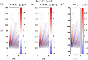
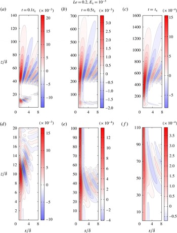
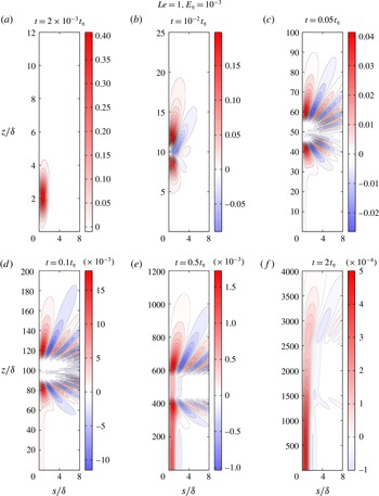
1 Introduction
It is well known that magnetohydrodynamic (MHD) turbulence differs from conventional turbulence in two ways: the magnetic field makes the flow anisotropic in the sense that the velocity gradient in the direction parallel to the field is significantly reduced, and the induced electric currents in the fluid cause ohmic dissipation of energy. The energy decay and anisotropy in freely decaying MHD turbulence have been measured in laboratory experiments (Alemany et al.
Reference Alemany, Moreau, Sulem and Frisch1979; Sreenivasan & Alboussière Reference Sreenivasan and Alboussière2002) operating in the limit of low magnetic Reynolds number,
 $Rm=u\unicode[STIX]{x1D6FF}/\unicode[STIX]{x1D702}\ll 1$
, where
 $u$
is the root mean square (r.m.s.) velocity of flow structures of length scale
 $\unicode[STIX]{x1D6FF}$
and
 $\unicode[STIX]{x1D702}$
is the magnetic diffusivity. Experiments on rotating liquid metal MHD turbulence at
 $Rm\sim 0.1$
(Brito et al.
Reference Brito, Cardin, Nataf and Marolleau1995) and
 $Rm\sim 10$
(Brito et al.
Reference Brito, Alboussiére, Cardin, Gagnière, Jault, Rizza, Masson, Nataf and Schmitt2011) reproduce the magnetostrophic regime where the ratio of the magnetic to Coriolis forces is of order unity, although the laws of energy decay in this regime are not known. Rapid rotation of the Earth’s outer core gives rise to thin convection columns aligned with the rotation axis (Busse Reference Busse1970) for which
 $Rm$
is naturally small. While
 $Rm$
based on the length scale of the Earth’s outer core (
 ${\sim}10^{3}~\text{km}$
) is possibly
 ${\sim}10^{3}$
(Olson Reference Olson and Olson2015), small-scale motions of
 $Rm\sim 1$
may be important for magnetic field generation within the core. The interaction between the small-scale velocity and the small-scale magnetic field gives rise to a large-scale mean magnetic field (Steenbeck, Krause & Rädler Reference Steenbeck, Krause and Rädler1966), a mechanism that finds support from dynamo experiments (Stieglitz & Müller Reference Stieglitz and Müller2001). In the Earth-like regime of rapid rotation and small nonlinear inertia, the backreaction of the magnetic field generates kinetic helicity whereby an axial dipole field holds itself up (Sreenivasan & Jones Reference Sreenivasan and Jones2011), and, notably, this process may occur in columns whose transverse length scales are largely determined by the rotation rate (Sreenivasan & Gopinath Reference Sreenivasan and Gopinath2017). Because the small scales of the velocity and the magnetic field in the core cannot be resolved from analysis of the secular variation of the Earth’s field (e.g. Kono & Roberts Reference Kono and Roberts2002), either rapidly rotating dynamo models or low-
 $Rm$
core turbulence models are needed to understand the dynamics of the small scales. Recent studies have proposed that ohmic dissipation in the core is maximum at length scales for which
 $Rm\sim 1$
, and much smaller length scales may support Alfvén waves (Nataf & Schaeffer Reference Nataf, Schaeffer and Olson2015). In addition, it is clear from numerical simulations of the geodynamo (Sreenivasan Reference Sreenivasan2010; Soderlund, King & Aurnou Reference Soderlund, King and Aurnou2012; Gopinath & Sreenivasan Reference Gopinath and Sreenivasan2015) that the self-generated magnetic field does not significantly increase the length scale of convection so as to render small scales unimportant. Convective vortices of
 $Rm\sim 1$
or less can therefore exist, for which the low-
 $Rm$
approximation gives a good qualitative description (Moffatt & Loper Reference Moffatt and Loper1994).
An early study by Lehnert (Reference Lehnert1955) considered the effect of a mean magnetic field on small-scale turbulence with and without background rotation. In particular, the behaviour of the solution is determined by the magnitude of a parameter that measures the ratio of the Alfvén wave frequency to the diffusion frequency,
 $$\begin{eqnarray}\unicode[STIX]{x1D701}=\frac{2\boldsymbol{B}\boldsymbol{\cdot }\boldsymbol{k}}{(\unicode[STIX]{x1D707}\unicode[STIX]{x1D70C})^{1/2}(\unicode[STIX]{x1D702}-\unicode[STIX]{x1D708})k^{2}},\end{eqnarray}$$
where
 $\boldsymbol{B}$
is the uniform mean magnetic field,
 $\boldsymbol{k}$
is the wave vector,
 $\unicode[STIX]{x1D707}$
is the magnetic permeability,
 $\unicode[STIX]{x1D70C}$
is the density and
 $\unicode[STIX]{x1D708}$
is the kinematic viscosity. For
 $|\unicode[STIX]{x1D701}|>1$
, a damped oscillatory solution occurs. Without rotation,
 $|\unicode[STIX]{x1D701}|=1$
marks the transition to a decaying solution, signifying pure diffusion. Crucially, with rotation, Lehnert found that the transition from periodic to aperiodic motions is displaced from
 $|\unicode[STIX]{x1D701}|=1$
to
 $|\unicode[STIX]{x1D701}|<1$
. The important role of the Coriolis force in delaying the wave–diffusion transition has not been addressed in the literature on MHD turbulence since the work of Lehnert. Moffatt (Reference Moffatt1967) looked at the long-time decay of an initial (non-rotating) turbulence for
 $|\unicode[STIX]{x1D701}|\gg 1$
and obtained the decay of kinetic and magnetic energies in the damped Alfvén wave phase and the subsequent phase of pure diffusion.
Analysis in the purely diffusive phase of MHD is considerably simplified through the quasistatic (
 $qs$
) approximation (Roberts Reference Roberts1967), where the rate of change of the induced field
 $\boldsymbol{b}$
is considered to be small in comparison with the diffusion frequency
 $\unicode[STIX]{x1D702}k^{2}$
in the limit of
 $Rm\ll 1$
. The
 $qs$
approximation is justified by most laboratory experiments with liquid metals, except in situations where Alfvén waves are generated (Jameson Reference Jameson1961; Alboussière et al.
Reference Alboussière, Cardin, Debray, Rizza, Masson, Plunian, Ribeiro and Schmitt2011). Simplified models of small-scale turbulence in the Earth’s core largely follow the
 $qs$
approximation (Braginsky & Meytlis Reference Braginsky and Meytlis1990; St. Pierre Reference St. Pierre1996; Siso-Nadal, Davidson & Graham Reference Siso-Nadal, Davidson and Graham2003; Siso-Nadal & Davidson Reference Siso-Nadal and Davidson2004), where the picture is that of linear inertial waves along the rotation axis and pseudodiffusion of momentum along the magnetic field lines. With the background rotation
 $\unicode[STIX]{x1D734}$
orthogonal to
 $\boldsymbol{B}$
, the long-time structure of the turbulence at low
 $Rm$
is that of platelets on
 $\boldsymbol{B}$
–
 $\unicode[STIX]{x1D734}$
planes (St. Pierre Reference St. Pierre1996; Siso-Nadal & Davidson Reference Siso-Nadal and Davidson2004).
In the presence of strong rotation, the consequences of neglecting
 $\unicode[STIX]{x2202}\boldsymbol{b}/\unicode[STIX]{x2202}t$
in the induction equation via the
 $qs$
approximation may be serious. First, the passage from the damped wave phase to the subsequent diffusive phase may be significantly delayed by rotation, which makes the wave phase an important part of rotating MHD turbulence. The decay of turbulence dominated by magneto-Coriolis (MC) waves has not received much theoretical attention. Second, the balance between the magnetic, buoyancy and Coriolis forces in rapidly rotating dynamos gives rise to slow magnetostrophic waves which are suppressed in
 $qs$
models. While the regime of occurrence of magnetostrophic waves in rotating MHD turbulence has been identified as large scale (Galtier Reference Galtier2014), and these waves appear in low-inertia geodynamo models (e.g. Hori, Jones & Teed Reference Hori, Jones and Teed2015), it is not known whether small scales of
 $Rm\sim 1$
or less that form in rapidly rotating planetary core convection can give rise to these waves in the presence of a mean magnetic field. It is therefore essential that simplified models of MHD turbulence that include the dynamics of damped MC waves are developed. The present study is a first step in this direction.
Motivated by the early studies of freely decaying small-scale turbulence under a magnetic field (Lehnert Reference Lehnert1955; Moffatt Reference Moffatt1967), we consider the long-time evolution of an isolated vortex at
 $Rm\ll 1$
. In this limit, the induced field
 $\boldsymbol{b}(\boldsymbol{x},t)$
satisfies the following linearized induction equation:
 $$\begin{eqnarray}\frac{\unicode[STIX]{x2202}\boldsymbol{b}}{\unicode[STIX]{x2202}t}=(\boldsymbol{B}\boldsymbol{\cdot }\unicode[STIX]{x1D735})\boldsymbol{u}+\unicode[STIX]{x1D702}\unicode[STIX]{x1D6FB}^{2}\boldsymbol{b}.\end{eqnarray}$$
In addition, the eddy turnover time
 $\unicode[STIX]{x1D6FF}/u$
is considered to be large compared with the Joule time
 $\unicode[STIX]{x1D70F}=\unicode[STIX]{x1D707}\unicode[STIX]{x1D702}\unicode[STIX]{x1D70C}/B^{2}$
as well as the rotation time
 $(2\unicode[STIX]{x1D6FA})^{-1}$
(where
 $\unicode[STIX]{x1D6FA}$
is the rotation rate), which essentially translates to the conditions of large magnetic interaction parameter
 $N$
and small Rossby number
 $Ro$
,
 $$\begin{eqnarray}N=\frac{B^{2}\unicode[STIX]{x1D6FF}}{\unicode[STIX]{x1D707}\unicode[STIX]{x1D702}\unicode[STIX]{x1D70C}u}\gg 1,\quad Ro=\frac{u}{2\unicode[STIX]{x1D6FA}\unicode[STIX]{x1D6FF}}\ll 1.\end{eqnarray}$$
These conditions imply that the nonlinear part of the inertial force is small compared with the Coriolis and Lorentz forces in the following equation of motion:
 $$\begin{eqnarray}\frac{\unicode[STIX]{x2202}\boldsymbol{u}}{\unicode[STIX]{x2202}t}=-\frac{1}{\unicode[STIX]{x1D70C}}\unicode[STIX]{x1D735}p^{\ast }+\frac{1}{\unicode[STIX]{x1D707}\unicode[STIX]{x1D70C}}(\boldsymbol{B}\boldsymbol{\cdot }\unicode[STIX]{x1D735})\boldsymbol{b}-2\unicode[STIX]{x1D734}\times \boldsymbol{u}+\unicode[STIX]{x1D708}\unicode[STIX]{x1D6FB}^{2}\boldsymbol{u},\end{eqnarray}$$
where
 $p^{\ast }=p-(\unicode[STIX]{x1D70C}/2)|\unicode[STIX]{x1D734}\times \boldsymbol{x}|^{2}+\boldsymbol{b}^{2}/2\unicode[STIX]{x1D707}$
. Equations (1.4) and (1.2) admit damped MC waves for a period of time; then, a diffusion-dominated phase ensues. An important aim of this study is to examine the wave phase of decay and the time scale for the wave–diffusion phase transition.
In § 2, the problem of long-time evolution of a flow structure and its general solutions are presented. Section 3 investigates the regime of strong background rotation, where the inertial wave frequency is much higher than the Alfvén wave frequency. The decay laws in the wave-dominated phase and the subsequent diffusion-dominated phase are obtained, followed by the wave–diffusion transition time scales. Two dimensionless parameters emerge from this analysis: the ratio of the inertial wave to Alfvén wave time scales,
 $Le$
, and the ratio of the inertial wave to magnetic diffusion time scales,
 $E_{\unicode[STIX]{x1D702}}$
, which are expressible in terms of the parameters
 $Rm$
,
 $N$
and
 $Ro$
by
 $Le^{2}=NRo^{2}\,Rm^{-1}$
and
 $E_{\unicode[STIX]{x1D702}}=Ro\,Rm^{-1}$
. Section 4 considers the regime of weak rotation, where the Alfvén wave frequency is much higher than the inertial wave frequency. Section 5 examines the computed general solutions of the initial value problem in § 2. Apart from verifying the decay laws obtained for the regime of strong rotation, these solutions bring out the difference between the decay patterns of fast and slow MC waves. Section 6 discusses some implications of this study for rotating planetary cores.
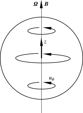
Schematic of an initial disturbance in a quiescent fluid subject to background rotation and a uniform axial magnetic field.

2 Problem set-up and general solutions
In this study, we consider the long-time damping of an initially localized disturbance in an incompressible rotating fluid threaded by a uniform magnetic field
 $\boldsymbol{B}=B_{0}\hat{\boldsymbol{e}}_{\boldsymbol{z}}$
. In cylindrical polar coordinates (
 $s,\unicode[STIX]{x1D719},z$
), the initial velocity field is taken to be symmetric about its own axis (independent of
 $\unicode[STIX]{x1D719}$
) and of the form
 $\boldsymbol{u}=(0,u_{\unicode[STIX]{x1D719}0},0)$
, where
 $$\begin{eqnarray}u_{\unicode[STIX]{x1D719}0}=As\exp [-(s^{2}+z^{2})/\unicode[STIX]{x1D6FF}^{2}].\end{eqnarray}$$
Here,
 $A$
is a constant and
 $\unicode[STIX]{x1D6FF}$
is the length scale of the flow. Figure 1 shows this initial blob of fluid, which subsequently evolves under the influence of coaxial background rotation
 $\unicode[STIX]{x1D734}$
and mean magnetic field
 $\boldsymbol{B}$
. Since equations (1.4) and (1.2) together lead to equation (A 1) for the velocity transform (appendix A) that admits plane wave solutions, the general solution for the toroidal velocity transform is given by
 $$\begin{eqnarray}\hat{u} _{\unicode[STIX]{x1D719}}=A_{1}\text{e}^{\text{i}\unicode[STIX]{x1D706}_{1}t}+B_{1}\text{e}^{\text{i}\unicode[STIX]{x1D706}_{2}t}+C_{1}\text{e}^{\text{i}\unicode[STIX]{x1D706}_{3}t}+D_{1}\text{e}^{\text{i}\unicode[STIX]{x1D706}_{4}t},\end{eqnarray}$$
where
 $\unicode[STIX]{x1D706}_{1-4}$
are the damped MC wave frequencies (appendix A). Here,
 $\unicode[STIX]{x1D706}_{1,2}$
represent fast inertial waves weakly modified by the mean magnetic field whereas
 $\unicode[STIX]{x1D706}_{3,4}$
represent slow magnetostrophic waves (Lehnert Reference Lehnert1954; Acheson & Hide Reference Acheson and Hide1973). For simplicity, these waves are henceforth called fast and slow MC waves. In (2.2),
 $A_{1}$
,
 $B_{1}$
,
 $C_{1}$
and
 $D_{1}$
are functions of the wavenumbers
 $k_{s}$
and
 $k_{z}$
and are evaluated from the initial (
 $t=0$
) conditions for
 $\hat{u} _{\unicode[STIX]{x1D719}}$
and its time derivatives.
From similar arguments, the general solution for the induced toroidal magnetic field transform is given by
 $$\begin{eqnarray}\hat{b}_{\unicode[STIX]{x1D719}}=A_{2}\text{e}^{\text{i}\unicode[STIX]{x1D706}_{1}t}+B_{2}\text{e}^{\text{i}\unicode[STIX]{x1D706}_{2}t}+C_{2}\text{e}^{\text{i}\unicode[STIX]{x1D706}_{3}t}+D_{2}\text{e}^{\text{i}\unicode[STIX]{x1D706}_{4}t},\end{eqnarray}$$
where
 $A_{2}$
,
 $B_{2}$
,
 $C_{2}$
and
 $D_{2}$
are evaluated from the initial conditions for
 $\hat{b}_{\unicode[STIX]{x1D719}}$
and its time derivatives.
2.1 Solutions of the initial value problem
The Hankel–Fourier transform
 $$\begin{eqnarray}\hat{\boldsymbol{f}}(k_{s},k_{z})=\frac{1}{2\unicode[STIX]{x03C0}^{2}}\int _{0}^{\infty }\int _{0}^{\infty }\boldsymbol{f}(s,z)\text{J}_{1}(k_{s}s)\text{e}^{-\text{i}k_{z}z}s\,\text{d}s\,\text{d}z,\end{eqnarray}$$
where
 $\text{J}_{1}$
is the Bessel function of the first kind of order one, is applied to the toroidal components of (1.4) and (1.2),
 $$\begin{eqnarray}\displaystyle & \displaystyle \frac{\unicode[STIX]{x2202}\hat{u} _{\unicode[STIX]{x1D719}}}{\unicode[STIX]{x2202}t}=\frac{B_{0}\text{i}k_{z}}{\unicode[STIX]{x1D707}\unicode[STIX]{x1D70C}}\hat{b}_{\unicode[STIX]{x1D719}}-2\unicode[STIX]{x1D6FA}\hat{u} _{s}-\unicode[STIX]{x1D708}k^{2}\hat{u} _{\unicode[STIX]{x1D719}}, & \displaystyle\end{eqnarray}$$
 $$\begin{eqnarray}\displaystyle & \displaystyle \frac{\unicode[STIX]{x2202}\hat{b}_{\unicode[STIX]{x1D719}}}{\unicode[STIX]{x2202}t}=B_{0}\text{i}k_{z}\hat{u} _{\unicode[STIX]{x1D719}}-\unicode[STIX]{x1D702}k^{2}\hat{b}_{\unicode[STIX]{x1D719}}, & \displaystyle\end{eqnarray}$$
where
 $k^{2}=k_{s}^{2}+k_{z}^{2}$
.
From (2.2), the initial conditions for
 $\hat{u} _{\unicode[STIX]{x1D719}}$
and its time derivatives are given by
 $$\begin{eqnarray}\left.\begin{array}{@{}c@{}}\displaystyle A_{1}+B_{1}+C_{1}+D_{1}=\hat{u} _{\unicode[STIX]{x1D719}0}=a_{1},\\ \displaystyle A_{1}\unicode[STIX]{x1D706}_{1}+B_{1}\unicode[STIX]{x1D706}_{2}+C_{1}\unicode[STIX]{x1D706}_{3}+D_{1}\unicode[STIX]{x1D706}_{4}=-\text{i}\left(\frac{\unicode[STIX]{x2202}\hat{u} _{\unicode[STIX]{x1D719}}}{\unicode[STIX]{x2202}t}\right)_{\!\!0}=a_{2},\\ \displaystyle A_{1}\unicode[STIX]{x1D706}_{1}^{2}+B_{1}\unicode[STIX]{x1D706}_{2}^{2}+C_{1}\unicode[STIX]{x1D706}_{3}^{2}+D_{1}\unicode[STIX]{x1D706}_{4}^{2}=-\left(\frac{\unicode[STIX]{x2202}^{2}\hat{u} _{\unicode[STIX]{x1D719}}}{\unicode[STIX]{x2202}t^{2}}\right)_{\!\!0}=a_{3},\\ \displaystyle A_{1}\unicode[STIX]{x1D706}_{1}^{3}+B_{1}\unicode[STIX]{x1D706}_{2}^{3}+C_{1}\unicode[STIX]{x1D706}_{3}^{3}+D_{1}\unicode[STIX]{x1D706}_{4}^{3}=\text{i}\!\left(\frac{\unicode[STIX]{x2202}^{3}\hat{u} _{\unicode[STIX]{x1D719}}}{\unicode[STIX]{x2202}t^{3}}\right)_{\!\!0}=a_{4}.\end{array}\right\}\end{eqnarray}$$
While the Hankel–Fourier transform of the initial condition (2.1) gives
 $\hat{u} _{\unicode[STIX]{x1D719}0}$
(Abramovitz & Stegun Reference Abramovitz and Stegun1965), two other physical conditions are necessary to evaluate the initial time derivatives: (i) the initial poloidal velocity is zero, so that
 $\hat{u} _{s0}=0$
, and (ii) if the mean magnetic field is taken to be switched on at the instant
 $t=0$
, the magnetic field perturbation takes finite time to develop by induction, so
 $\hat{b}_{\unicode[STIX]{x1D719}0}=0$
. Algebraic simplifications using (2.5) and (2.6) give the right-hand sides of (2.7) as follows:
 $$\begin{eqnarray}\displaystyle & \displaystyle a_{1}=\hat{u} _{\unicode[STIX]{x1D719}0}=\frac{k_{s}\unicode[STIX]{x1D6FF}^{5}}{16\unicode[STIX]{x03C0}^{3/2}}\text{e}^{-k^{2}\unicode[STIX]{x1D6FF}^{2}/4}, & \displaystyle\end{eqnarray}$$
 $$\begin{eqnarray}\displaystyle & \displaystyle a_{2}=\text{i}\unicode[STIX]{x1D708}k^{2}\hat{u} _{\unicode[STIX]{x1D719}0}, & \displaystyle\end{eqnarray}$$
 $$\begin{eqnarray}\displaystyle & \displaystyle a_{3}=\left(V_{A}^{2}k_{z}^{2}+\frac{4\unicode[STIX]{x1D6FA}^{2}k_{z}^{2}}{k^{2}}-\unicode[STIX]{x1D708}^{2}k^{4}\right)\hat{u} _{\unicode[STIX]{x1D719}0}, & \displaystyle\end{eqnarray}$$
 $$\begin{eqnarray}\displaystyle & \displaystyle a_{4}=\text{i}[(2\unicode[STIX]{x1D708}+\unicode[STIX]{x1D702})V_{A}^{2}k_{z}^{2}k^{2}+12\unicode[STIX]{x1D6FA}^{2}\unicode[STIX]{x1D708}k_{z}^{2}-\unicode[STIX]{x1D708}^{3}k^{6}]\hat{u} _{\unicode[STIX]{x1D719}0}, & \displaystyle\end{eqnarray}$$
where
 $V_{A}=B_{0}/\sqrt{\unicode[STIX]{x1D707}\unicode[STIX]{x1D70C}}$
is the Alfvén velocity. Equations (2.8)–(2.11) in turn give
 $$\begin{eqnarray}\left.\begin{array}{@{}c@{}}\displaystyle A_{1}=\frac{a_{4}-a_{3}(\unicode[STIX]{x1D706}_{2}+\unicode[STIX]{x1D706}_{3}+\unicode[STIX]{x1D706}_{4})+a_{2}[\unicode[STIX]{x1D706}_{2}(\unicode[STIX]{x1D706}_{3}+\unicode[STIX]{x1D706}_{4})+\unicode[STIX]{x1D706}_{3}\unicode[STIX]{x1D706}_{4}]-a_{1}\unicode[STIX]{x1D706}_{3}\unicode[STIX]{x1D706}_{4}\unicode[STIX]{x1D706}_{2}}{(\unicode[STIX]{x1D706}_{1}-\unicode[STIX]{x1D706}_{2})(\unicode[STIX]{x1D706}_{1}-\unicode[STIX]{x1D706}_{3})(\unicode[STIX]{x1D706}_{1}-\unicode[STIX]{x1D706}_{4})},\\ \displaystyle B_{1}=\frac{a_{4}-a_{3}(\unicode[STIX]{x1D706}_{1}+\unicode[STIX]{x1D706}_{3}+\unicode[STIX]{x1D706}_{4})+a_{2}[\unicode[STIX]{x1D706}_{1}(\unicode[STIX]{x1D706}_{3}+\unicode[STIX]{x1D706}_{4})+\unicode[STIX]{x1D706}_{3}\unicode[STIX]{x1D706}_{4}]-a_{1}\unicode[STIX]{x1D706}_{3}\unicode[STIX]{x1D706}_{4}\unicode[STIX]{x1D706}_{1}}{(\unicode[STIX]{x1D706}_{2}-\unicode[STIX]{x1D706}_{1})(\unicode[STIX]{x1D706}_{2}-\unicode[STIX]{x1D706}_{3})(\unicode[STIX]{x1D706}_{2}-\unicode[STIX]{x1D706}_{4})},\\ \displaystyle C_{1}=\frac{a_{4}-a_{3}(\unicode[STIX]{x1D706}_{1}+\unicode[STIX]{x1D706}_{2}+\unicode[STIX]{x1D706}_{4})+a_{2}[\unicode[STIX]{x1D706}_{1}(\unicode[STIX]{x1D706}_{2}+\unicode[STIX]{x1D706}_{4})+\unicode[STIX]{x1D706}_{2}\unicode[STIX]{x1D706}_{4}]-a_{1}\unicode[STIX]{x1D706}_{2}\unicode[STIX]{x1D706}_{4}\unicode[STIX]{x1D706}_{1}}{(\unicode[STIX]{x1D706}_{3}-\unicode[STIX]{x1D706}_{4})(\unicode[STIX]{x1D706}_{3}-\unicode[STIX]{x1D706}_{1})(\unicode[STIX]{x1D706}_{3}-\unicode[STIX]{x1D706}_{2})},\\ \displaystyle D_{1}=\frac{a_{4}-a_{3}(\unicode[STIX]{x1D706}_{1}+\unicode[STIX]{x1D706}_{2}+\unicode[STIX]{x1D706}_{3})+a_{2}[\unicode[STIX]{x1D706}_{1}(\unicode[STIX]{x1D706}_{2}+\unicode[STIX]{x1D706}_{3})+\unicode[STIX]{x1D706}_{2}\unicode[STIX]{x1D706}_{3}]-a_{1}\unicode[STIX]{x1D706}_{2}\unicode[STIX]{x1D706}_{3}\unicode[STIX]{x1D706}_{1}}{(\unicode[STIX]{x1D706}_{4}-\unicode[STIX]{x1D706}_{3})(\unicode[STIX]{x1D706}_{4}-\unicode[STIX]{x1D706}_{2})(\unicode[STIX]{x1D706}_{4}-\unicode[STIX]{x1D706}_{1})}.\end{array}\right\}\end{eqnarray}$$
From (2.3), the initial conditions for
 $\hat{b}_{\unicode[STIX]{x1D719}}$
and its time derivatives are given by
 $$\begin{eqnarray}\left.\begin{array}{@{}c@{}}\displaystyle A_{2}+B_{2}+C_{2}+D_{2}=\hat{b}_{\unicode[STIX]{x1D719}0}=b_{1},\\ \displaystyle A_{2}\unicode[STIX]{x1D706}_{1}+B_{2}\unicode[STIX]{x1D706}_{2}+C_{2}\unicode[STIX]{x1D706}_{3}+D_{2}\unicode[STIX]{x1D706}_{4}=-\text{i}\!\left(\frac{\unicode[STIX]{x2202}\hat{b}_{\unicode[STIX]{x1D719}}}{\unicode[STIX]{x2202}t}\right)_{\!\!0}=b_{2},\\ \displaystyle A_{2}\unicode[STIX]{x1D706}_{1}^{2}+B_{2}\unicode[STIX]{x1D706}_{2}^{2}+C_{2}\unicode[STIX]{x1D706}_{3}^{2}+D_{2}\unicode[STIX]{x1D706}_{4}^{2}=-\left(\frac{\unicode[STIX]{x2202}^{2}\hat{b}_{\unicode[STIX]{x1D719}}}{\unicode[STIX]{x2202}t^{2}}\right)_{\!\!0}=b_{3},\\ \displaystyle A_{2}\unicode[STIX]{x1D706}_{1}^{3}+B_{2}\unicode[STIX]{x1D706}_{2}^{3}+C_{2}\unicode[STIX]{x1D706}_{3}^{3}+D_{2}\unicode[STIX]{x1D706}_{4}^{3}=\text{i}\!\left(\frac{\unicode[STIX]{x2202}^{3}\hat{b}_{\unicode[STIX]{x1D719}}}{\unicode[STIX]{x2202}t^{3}}\right)_{\!\!0}=b_{4}.\end{array}\right\}\end{eqnarray}$$
The right-hand sides of (2.13) are obtained as follows:
 $$\begin{eqnarray}\displaystyle & \displaystyle b_{1}=0, & \displaystyle\end{eqnarray}$$
 $$\begin{eqnarray}\displaystyle & \displaystyle b_{2}=B_{0}k_{z}\hat{u} _{\unicode[STIX]{x1D719}0}, & \displaystyle\end{eqnarray}$$
 $$\begin{eqnarray}\displaystyle & \displaystyle b_{3}=\text{i}(\unicode[STIX]{x1D708}+\unicode[STIX]{x1D702})B_{0}k_{z}k^{2}\hat{u} _{\unicode[STIX]{x1D719}0}, & \displaystyle\end{eqnarray}$$
 $$\begin{eqnarray}\displaystyle & \displaystyle b_{4}=B_{0}k_{z}\left[V_{A}^{2}k_{z}^{2}+\frac{4\unicode[STIX]{x1D6FA}^{2}k_{z}^{2}}{k^{2}}-k^{4}(\unicode[STIX]{x1D708}^{2}+\unicode[STIX]{x1D702}^{2}+\unicode[STIX]{x1D708}\unicode[STIX]{x1D702})\right]\hat{u} _{\unicode[STIX]{x1D719}0}, & \displaystyle\end{eqnarray}$$
which in turn give
 $$\begin{eqnarray}\left.\begin{array}{@{}c@{}}\displaystyle A_{2}=\frac{b_{4}-b_{3}(\unicode[STIX]{x1D706}_{2}+\unicode[STIX]{x1D706}_{3}+\unicode[STIX]{x1D706}_{4})+b_{2}[\unicode[STIX]{x1D706}_{2}(\unicode[STIX]{x1D706}_{3}+\unicode[STIX]{x1D706}_{4})+\unicode[STIX]{x1D706}_{3}\unicode[STIX]{x1D706}_{4}]}{(\unicode[STIX]{x1D706}_{1}-\unicode[STIX]{x1D706}_{2})(\unicode[STIX]{x1D706}_{1}-\unicode[STIX]{x1D706}_{3})(\unicode[STIX]{x1D706}_{1}-\unicode[STIX]{x1D706}_{4})},\\ \displaystyle B_{2}=\frac{b_{4}-b_{3}(\unicode[STIX]{x1D706}_{1}+\unicode[STIX]{x1D706}_{3}+\unicode[STIX]{x1D706}_{4})+b_{2}[\unicode[STIX]{x1D706}_{1}(\unicode[STIX]{x1D706}_{3}+\unicode[STIX]{x1D706}_{4})+\unicode[STIX]{x1D706}_{3}\unicode[STIX]{x1D706}_{4}]}{(\unicode[STIX]{x1D706}_{2}-\unicode[STIX]{x1D706}_{1})(\unicode[STIX]{x1D706}_{2}-\unicode[STIX]{x1D706}_{3})(\unicode[STIX]{x1D706}_{2}-\unicode[STIX]{x1D706}_{4})},\\ \displaystyle C_{2}=\frac{b_{4}-b_{3}(\unicode[STIX]{x1D706}_{1}+\unicode[STIX]{x1D706}_{2}+\unicode[STIX]{x1D706}_{4})+b_{2}[\unicode[STIX]{x1D706}_{1}(\unicode[STIX]{x1D706}_{2}+\unicode[STIX]{x1D706}_{4})+\unicode[STIX]{x1D706}_{2}\unicode[STIX]{x1D706}_{4}]}{(\unicode[STIX]{x1D706}_{3}-\unicode[STIX]{x1D706}_{4})(\unicode[STIX]{x1D706}_{3}-\unicode[STIX]{x1D706}_{1})(\unicode[STIX]{x1D706}_{3}-\unicode[STIX]{x1D706}_{2})},\\ \displaystyle D_{2}=\frac{b_{4}-b_{3}(\unicode[STIX]{x1D706}_{1}+\unicode[STIX]{x1D706}_{2}+\unicode[STIX]{x1D706}_{3})+b_{2}[\unicode[STIX]{x1D706}_{1}(\unicode[STIX]{x1D706}_{2}+\unicode[STIX]{x1D706}_{3})+\unicode[STIX]{x1D706}_{2}\unicode[STIX]{x1D706}_{3}]}{(\unicode[STIX]{x1D706}_{4}-\unicode[STIX]{x1D706}_{3})(\unicode[STIX]{x1D706}_{4}-\unicode[STIX]{x1D706}_{2})(\unicode[STIX]{x1D706}_{4}-\unicode[STIX]{x1D706}_{1})}.\end{array}\right\}\end{eqnarray}$$
For a given time, the toroidal velocity and magnetic fields in real space (
 $u_{\unicode[STIX]{x1D719}}$
,
 $b_{\unicode[STIX]{x1D719}}$
) may now be recovered from (2.2) and (2.3) by the inverse Hankel–Fourier transform,
 $$\begin{eqnarray}\boldsymbol{f}(s,z)=4\unicode[STIX]{x03C0}\int _{0}^{\infty }\int _{0}^{\infty }\hat{\boldsymbol{f}}(k_{s},k_{z})\text{J}_{1}(k_{s}s)\text{e}^{\text{i}k_{z}z}k_{s}\,\text{d}k_{s}\,\text{d}k_{z}.\end{eqnarray}$$
Although the Coriolis force generates poloidal components of
 $\hat{\boldsymbol{u}}$
and hence
 $\hat{\boldsymbol{b}}$
, we shall see in § 5 that for
 $Ro\ll 1$
, background rotation equalizes the toroidal and poloidal energies regardless of whether the inertial wave frequency is higher or lower in magnitude than the Alfvén wave frequency. It is therefore possible to study magnetic damping of the system by looking at the evolution of the toroidal components of the fields,
 $\hat{u} _{\unicode[STIX]{x1D719}}$
and
 $\hat{b}_{\unicode[STIX]{x1D719}}$
. Before looking at the computed general solutions of our initial value problem, we discuss approximate analytical solutions in the inviscid limit (
 $\unicode[STIX]{x1D708}=0$
) that provide long-time decay laws for the kinetic and magnetic energies of the system. The decay begins in a wave-dominated phase that lasts for a significant period of time, and subsequently enters a diffusion-dominated phase. First, we consider the regime of strong rotation where the inertial wave frequency
 $\unicode[STIX]{x1D6FA}k_{z}/k$
is much higher in magnitude than the Alfvén wave frequency
 $V_{A}k_{z}$
.
3 Strong rotation: approximate analytical solutions
In the inviscid limit, the relative orders of magnitude of the fundamental frequencies in the two phases of decay are given by the following inequalities:
-
(i)
 $\unicode[STIX]{x1D6FA}k_{z}/k\gg V_{A}k_{z}\gg \unicode[STIX]{x1D702}k^{2}/2$
(wave-dominated phase);
-
(ii)
$\unicode[STIX]{x1D702}k^{2}/2\gg \unicode[STIX]{x1D6FA}k_{z}/k\gg V_{A}k_{z}$
(diffusion-dominated phase).


We begin by obtaining approximations for the fast (
 $\unicode[STIX]{x1D706}_{1,2}$
) and slow (
 $\unicode[STIX]{x1D706}_{3,4}$
) MC wave frequencies in the two phases.
3.1 Frequency approximations in the wave-dominated phase
Noting that
 $\unicode[STIX]{x1D6FA}k_{z}/k$
is the dominant frequency in this phase, the fast MC wave frequency
 $\unicode[STIX]{x1D706}_{1}$
(appendix A) in the inviscid limit (
 $\unicode[STIX]{x1D708}=0$
) is rewritten in the form
 $$\begin{eqnarray}\unicode[STIX]{x1D706}_{1}=\frac{\unicode[STIX]{x1D6FA}k_{z}}{k}+\text{i}\frac{\unicode[STIX]{x1D702}k^{2}}{2}+\frac{\unicode[STIX]{x1D6FA}k_{z}}{k}\sqrt{\left(\frac{V_{A}k}{\unicode[STIX]{x1D6FA}}\right)^{2}+1-\left(\frac{\unicode[STIX]{x1D702}k^{3}}{2\unicode[STIX]{x1D6FA}k_{z}}\right)^{2}-\text{i}\frac{\unicode[STIX]{x1D702}k^{3}}{\unicode[STIX]{x1D6FA}k_{z}}}.\end{eqnarray}$$
Since
 $\unicode[STIX]{x1D702}k^{3}/2\unicode[STIX]{x1D6FA}k_{z}\ll V_{A}k/\unicode[STIX]{x1D6FA}\ll 1$
,
 $$\begin{eqnarray}\unicode[STIX]{x1D706}_{1}\approx \frac{\unicode[STIX]{x1D6FA}k_{z}}{k}+\text{i}\frac{\unicode[STIX]{x1D702}k^{2}}{2}+\frac{\unicode[STIX]{x1D6FA}k_{z}}{k}\sqrt{1+\left(\frac{V_{A}k}{\unicode[STIX]{x1D6FA}}\right)^{2}-\text{i}\frac{\unicode[STIX]{x1D702}k^{3}}{\unicode[STIX]{x1D6FA}k_{z}}}.\end{eqnarray}$$
Letting
 $x=V_{A}k/\unicode[STIX]{x1D6FA}$
and
 $y=\unicode[STIX]{x1D702}k^{3}/\unicode[STIX]{x1D6FA}k_{z}$
in (3.2),
 $$\begin{eqnarray}\displaystyle \sqrt{1+x^{2}-\text{i}y} & = & \displaystyle \sqrt{1+x^{2}}\left[1-\text{i}\frac{y}{1+x^{2}}\right]^{1/2},\nonumber\\ \displaystyle & {\approx} & \displaystyle \sqrt{1+x^{2}}\left[1-\text{i}\frac{y}{2(1+x^{2})}\right],\nonumber\\ \displaystyle & {\approx} & \displaystyle 1+\frac{x^{2}}{2}-\text{i}\frac{y}{2}\left(1-\frac{x^{2}}{2}\right).\end{eqnarray}$$
Use of this approximation in (3.2) gives
 $$\begin{eqnarray}\unicode[STIX]{x1D706}_{1}\approx \frac{\unicode[STIX]{x1D6FA}k_{z}}{k}+\text{i}\frac{\unicode[STIX]{x1D702}k^{2}}{2}+\frac{\unicode[STIX]{x1D6FA}k_{z}}{k}\left[1+\frac{V_{A}^{2}k^{2}}{2\unicode[STIX]{x1D6FA}^{2}}-\text{i}\frac{\unicode[STIX]{x1D702}k^{3}}{2\unicode[STIX]{x1D6FA}k_{z}}\left(1-\frac{V_{A}^{2}k^{2}}{2\unicode[STIX]{x1D6FA}^{2}}\right)\right],\end{eqnarray}$$
and noting that the term containing
 $V_{A}^{2}k^{2}/2\unicode[STIX]{x1D6FA}^{2}$
is negligible in the real part of the frequency, we obtain
 $$\begin{eqnarray}\unicode[STIX]{x1D706}_{1}\approx \frac{2\unicode[STIX]{x1D6FA}k_{z}}{k}+\text{i}\frac{\unicode[STIX]{x1D702}V_{A}^{2}k^{4}}{4\unicode[STIX]{x1D6FA}^{2}}.\end{eqnarray}$$
In a similar way,
 $$\begin{eqnarray}\unicode[STIX]{x1D706}_{2}\approx -\frac{2\unicode[STIX]{x1D6FA}k_{z}}{k}+\text{i}\frac{\unicode[STIX]{x1D702}V_{A}^{2}k^{4}}{4\unicode[STIX]{x1D6FA}^{2}}.\end{eqnarray}$$
The slow MC wave frequency
 $\unicode[STIX]{x1D706}_{3}$
(appendix A) in the inviscid limit is rewritten in the form
 $$\begin{eqnarray}\unicode[STIX]{x1D706}_{3}=-\frac{\unicode[STIX]{x1D6FA}k_{z}}{k}+\text{i}\frac{\unicode[STIX]{x1D702}k^{2}}{2}+\frac{\unicode[STIX]{x1D6FA}k_{z}}{k}\sqrt{\left(\frac{V_{A}k}{\unicode[STIX]{x1D6FA}}\right)^{2}+1-\left(\frac{\unicode[STIX]{x1D702}k^{3}}{2\unicode[STIX]{x1D6FA}k_{z}}\right)^{2}+\text{i}\frac{\unicode[STIX]{x1D702}k^{3}}{\unicode[STIX]{x1D6FA}k_{z}}},\end{eqnarray}$$
approximated by
 $$\begin{eqnarray}\unicode[STIX]{x1D706}_{3}\approx -\frac{\unicode[STIX]{x1D6FA}k_{z}}{k}+\text{i}\frac{\unicode[STIX]{x1D702}k^{2}}{2}+\frac{\unicode[STIX]{x1D6FA}k_{z}}{k}\sqrt{1+\left(\frac{V_{A}k}{\unicode[STIX]{x1D6FA}}\right)^{2}+\text{i}\frac{\unicode[STIX]{x1D702}k^{3}}{\unicode[STIX]{x1D6FA}k_{z}}}\end{eqnarray}$$
and further simplified to
 $$\begin{eqnarray}\unicode[STIX]{x1D706}_{3}\approx \frac{V_{A}^{2}k_{z}k}{2\unicode[STIX]{x1D6FA}}+\text{i}\unicode[STIX]{x1D702}k^{2}.\end{eqnarray}$$
In a similar way,
 $$\begin{eqnarray}\unicode[STIX]{x1D706}_{4}\approx -\frac{V_{A}^{2}k_{z}k}{2\unicode[STIX]{x1D6FA}}+\text{i}\unicode[STIX]{x1D702}k^{2}.\end{eqnarray}$$
3.2 Frequency approximations in the diffusion-dominated phase
Noting that
 $\unicode[STIX]{x1D702}k^{2}/2$
is the dominant frequency in this phase, the fast MC wave frequency
 $\unicode[STIX]{x1D706}_{1}$
in the inviscid limit is rewritten in the form
 $$\begin{eqnarray}\unicode[STIX]{x1D706}_{1}=\frac{\unicode[STIX]{x1D6FA}k_{z}}{k}+\text{i}\frac{\unicode[STIX]{x1D702}k^{2}}{2}+\frac{\unicode[STIX]{x1D702}k^{2}}{2}\sqrt{\left(\frac{2V_{A}k_{z}}{\unicode[STIX]{x1D702}k^{2}}\right)^{2}+\left(\frac{2\unicode[STIX]{x1D6FA}k_{z}}{\unicode[STIX]{x1D702}k^{3}}-\text{i}\right)^{2}}.\end{eqnarray}$$
Since
 $2V_{A}k_{z}/\unicode[STIX]{x1D702}k^{2}\ll 2\unicode[STIX]{x1D6FA}k_{z}/\unicode[STIX]{x1D702}k^{3}\ll 1$
, further simplification gives
 $$\begin{eqnarray}\unicode[STIX]{x1D706}_{1}\approx \frac{2\unicode[STIX]{x1D6FA}k_{z}}{k}+\text{i}\frac{k_{z}^{2}}{\unicode[STIX]{x1D70F}k^{2}},\end{eqnarray}$$
where
 $\unicode[STIX]{x1D70F}=\unicode[STIX]{x1D702}/V_{A}^{2}$
is the Joule time. In a similar way,
 $$\begin{eqnarray}\unicode[STIX]{x1D706}_{2}\approx -\frac{2\unicode[STIX]{x1D6FA}k_{z}}{k}+\text{i}\frac{k_{z}^{2}}{\unicode[STIX]{x1D70F}k^{2}}.\end{eqnarray}$$
The slow MC wave frequency
 $\unicode[STIX]{x1D706}_{3}$
is rewritten in the form
 $$\begin{eqnarray}\unicode[STIX]{x1D706}_{3}=-\frac{\unicode[STIX]{x1D6FA}k_{z}}{k}+\text{i}\frac{\unicode[STIX]{x1D702}k^{2}}{2}+\frac{\unicode[STIX]{x1D702}k^{2}}{2}\sqrt{\left(\frac{2V_{A}k_{z}}{\unicode[STIX]{x1D702}k^{2}}\right)^{2}+\left(\frac{2\unicode[STIX]{x1D6FA}k_{z}}{\unicode[STIX]{x1D702}k^{3}}+\text{i}\right)^{2}}\end{eqnarray}$$
and approximated by
 $$\begin{eqnarray}\unicode[STIX]{x1D706}_{3}\approx \frac{2\unicode[STIX]{x1D6FA}V_{A}^{2}k_{z}^{3}}{\unicode[STIX]{x1D702}^{2}k^{5}}+\text{i}\unicode[STIX]{x1D702}k^{2}.\end{eqnarray}$$
In a similar way,
 $$\begin{eqnarray}\unicode[STIX]{x1D706}_{4}\approx -\frac{2\unicode[STIX]{x1D6FA}V_{A}^{2}k_{z}^{3}}{\unicode[STIX]{x1D702}^{2}k^{5}}+\text{i}\unicode[STIX]{x1D702}k^{2}.\end{eqnarray}$$
The
 $\unicode[STIX]{x1D706}_{1,2}$
frequency approximations (3.12) and (3.13) are the same as the frequencies
 $\unicode[STIX]{x1D706}_{qs}$
obtained directly from the dispersion relation in the quasistatic (
 $qs$
) limit (appendix A, equation (A 4) for
 $\unicode[STIX]{x1D708}=0$
), which indicates that the system undergoes transition to the diffusion-dominated
 $qs$
phase essentially via progressive damping of the fast MC wave.
The imaginary parts of
 $\unicode[STIX]{x1D706}_{3,4}$
in (3.9), (3.10) and (3.15), (3.16) indicate that the slow MC wave decay is isotropic throughout. In contrast, the imaginary parts of
 $\unicode[STIX]{x1D706}_{1,2}$
in (3.12) and (3.13) indicate that the fast MC wave decay is anisotropic in the diffusion-dominated phase. We shall return to this point in § 5.
3.3 Energy decay in the wave-dominated phase
We investigate the decay of kinetic and magnetic energies for the fast and slow MC wave components separately. As noted earlier, the inviscid (
 $\unicode[STIX]{x1D708}=0$
) limit is considered to focus attention on magnetic damping.
3.3.1 Fast wave kinetic energy
The velocity transform
 $\hat{u} _{\unicode[STIX]{x1D719},\text{f}}=A_{1}\text{e}^{\text{i}\unicode[STIX]{x1D706}_{1}t}$
representing the forward-travelling (
 $z>0$
) fast MC wave component is analysed, where
 $A_{1}$
is obtained from (2.12). Following algebraic simplifications using the frequency approximations (3.5), (3.6), (3.9) and (3.10) as well as the inequality
 $\unicode[STIX]{x1D6FA}k_{z}/k\gg V_{A}k_{z}\gg \unicode[STIX]{x1D702}k^{2}/2$
for the wave-dominated phase, we obtain
 $$\begin{eqnarray}\hat{u} _{\unicode[STIX]{x1D719},\text{f}}\approx \frac{\hat{u} _{\unicode[STIX]{x1D719}0}}{2}\exp \left(-\frac{\unicode[STIX]{x1D702}V_{A}^{2}k^{4}t}{4\unicode[STIX]{x1D6FA}^{2}}\right)\left[\cos \left(\frac{2\unicode[STIX]{x1D6FA}k_{z}t}{k}\right)-\frac{3\unicode[STIX]{x1D702}V_{A}^{2}k^{5}}{8\unicode[STIX]{x1D6FA}^{3}k_{z}}\sin \left(\frac{2\unicode[STIX]{x1D6FA}k_{z}t}{k}\right)\right]\end{eqnarray}$$
as the leading-order solution. It is notable that the fast wave undergoes diffusion on a time scale
 $$\begin{eqnarray}t_{1}=\frac{4\unicode[STIX]{x1D6FA}^{2}}{\unicode[STIX]{x1D702}V_{A}^{2}k_{0}^{4}},\end{eqnarray}$$
where
 $k_{0}$
is the initial wavenumber of the disturbance.
For
 $t\ll t_{1}$
,
 $\hat{u} _{\unicode[STIX]{x1D719},\text{f}}\approx \hat{u} _{\unicode[STIX]{x1D719}0}/2$
, so that the kinetic energy given by Parseval’s theorem,
 $$\begin{eqnarray}E_{\text{k},\text{f}}=16\unicode[STIX]{x03C0}^{4}\int _{0}^{\infty }\int _{0}^{\infty }|\hat{u} _{\unicode[STIX]{x1D719},\text{f}}|^{2}k_{s}\,\text{d}k_{s}\,\text{d}k_{z},\end{eqnarray}$$
simplifies to
 $$\begin{eqnarray}E_{\text{k},\text{f}}\approx \frac{\sqrt{2}\unicode[STIX]{x03C0}^{3/2}\unicode[STIX]{x1D6FF}^{5}}{64}=\frac{E_{0}}{4}\end{eqnarray}$$
by taking the expression for
 $\hat{u} _{\unicode[STIX]{x1D719}0}$
from equation (2.8). Here,
 $E_{0}$
is the initial kinetic energy of the disturbance.
For
 $t\gtrsim t_{1}$
, the kinetic energy is expanded as
 $$\begin{eqnarray}\displaystyle E_{\text{k},\text{f}} & {\approx} & \displaystyle 4\unicode[STIX]{x03C0}^{4}\int _{0}^{\infty }\int _{0}^{\infty }|\hat{u} _{\unicode[STIX]{x1D719}0}|^{2}\exp \left(-\frac{\unicode[STIX]{x1D702}V_{A}^{2}k^{4}t}{2\unicode[STIX]{x1D6FA}^{2}}\right)k_{s}\,\text{d}k_{s}\,\text{d}k_{z},\nonumber\\ \displaystyle & {\approx} & \displaystyle \frac{\unicode[STIX]{x03C0}\unicode[STIX]{x1D6FF}^{10}}{64}\int _{0}^{\infty }\int _{0}^{\infty }k_{s}^{3}\exp \left(-\frac{k^{2}\unicode[STIX]{x1D6FF}^{2}}{2}-\frac{\unicode[STIX]{x1D702}V_{A}^{2}k^{4}t}{2\unicode[STIX]{x1D6FA}^{2}}\right)\text{d}k_{s}\,\text{d}k_{z}.\end{eqnarray}$$
Using the substitutions
 $k_{s}=k\cos \unicode[STIX]{x1D703}$
and
 $k_{z}=k\sin \unicode[STIX]{x1D703}$
, we obtain
 $$\begin{eqnarray}\displaystyle E_{\text{k},\text{f}} & {\approx} & \displaystyle \frac{\unicode[STIX]{x03C0}\unicode[STIX]{x1D6FF}^{10}}{64}\int _{0}^{\unicode[STIX]{x03C0}/2}\cos ^{3}\unicode[STIX]{x1D703}\,\text{d}\unicode[STIX]{x1D703}\int _{0}^{\infty }k^{4}\exp \left(-\frac{k^{2}\unicode[STIX]{x1D6FF}^{2}}{2}-\frac{\unicode[STIX]{x1D702}V_{A}^{2}k^{4}t}{2\unicode[STIX]{x1D6FA}^{2}}\right)\,\text{d}k,\nonumber\\ \displaystyle & {\approx} & \displaystyle \frac{\unicode[STIX]{x03C0}\unicode[STIX]{x1D6FF}^{10}}{96}\int _{0}^{\infty }k^{4}\exp \left(-\frac{k^{2}\unicode[STIX]{x1D6FF}^{2}}{2}-\frac{\unicode[STIX]{x1D702}V_{A}^{2}k^{4}t}{2\unicode[STIX]{x1D6FA}^{2}}\right)\,\text{d}k.\end{eqnarray}$$
The integral in (3.22), of the form
 $$\begin{eqnarray}I_{A}=\int _{0}^{\infty }k^{4}\text{exp}(-ak^{2}-bk^{4})\,\text{d}k,\end{eqnarray}$$
where
 $a=\unicode[STIX]{x1D6FF}^{2}/2$
and
 $b=\unicode[STIX]{x1D702}V_{A}^{2}t/2\unicode[STIX]{x1D6FA}^{2}$
, has the following solution (B 4, appendix B):
 $$\begin{eqnarray}I_{A}=\frac{\sqrt{a}\exp (a^{2}/8b)}{32b^{5/2}}\left[(a^{2}+2b)\text{K}_{1/4}\left(\frac{a^{2}}{8b}\right)-a^{2}\text{K}_{3/4}\left(\frac{a^{2}}{8b}\right)\right],\end{eqnarray}$$
where
 $\text{K}_{n}(x)$
is the modified Bessel function of the second kind. In the limit
 $b\rightarrow \infty$
(
 $t\gg t_{1}$
),
 $I_{A}$
is approximated by (B 9, appendix B)
 $$\begin{eqnarray}I_{A}\approx \frac{\unicode[STIX]{x1D6E4}(1/4)b^{-5/4}}{16}+O(b^{-7/4}).\end{eqnarray}$$
Hence, the kinetic energy in this limit evolves as
 $$\begin{eqnarray}\displaystyle E_{\text{k},\text{f}} & {\approx} & \displaystyle \frac{\unicode[STIX]{x03C0}\unicode[STIX]{x1D6FF}^{10}}{96}\times \frac{\unicode[STIX]{x1D6E4}(1/4)b^{-5/4}}{16},\nonumber\\ \displaystyle & {\approx} & \displaystyle \frac{\unicode[STIX]{x03C0}\unicode[STIX]{x1D6FF}^{10}\unicode[STIX]{x1D6E4}(1/4)}{1536}\left(\frac{2t}{k_{0}^{4}t_{1}}\right)^{-5/4}.\end{eqnarray}$$
Since
 $k_{0}\unicode[STIX]{x1D6FF}=\sqrt{5}$
for our initial condition (2.1), the kinetic energy simplifies to
 $$\begin{eqnarray}E_{\text{k},\text{f}}\approx \frac{25\sqrt{5}\unicode[STIX]{x03C0}\unicode[STIX]{x1D6FF}^{5}\unicode[STIX]{x1D6E4}(1/4)}{2^{5/4}\times 1536}\left(\frac{t}{t_{1}}\right)^{-5/4}.\end{eqnarray}$$
For
 $t\gg t_{1}$
, the fast wave kinetic energy decays as
 $(t/t_{1})^{-5/4}$
.
3.3.2 Fast wave magnetic energy
The induced magnetic field transform
 $\hat{b}_{\unicode[STIX]{x1D719},\text{f}}=A_{2}\text{e}^{\text{i}\unicode[STIX]{x1D706}_{1}t}$
representing the fast MC wave component is analysed, where
 $A_{2}$
is obtained from (2.18). Following simplifications using the frequency approximations as in § 3.3.1, we obtain
 $$\begin{eqnarray}\hat{b}_{\unicode[STIX]{x1D719},\text{f}}\approx \text{i}\sqrt{\unicode[STIX]{x1D707}\unicode[STIX]{x1D70C}}\hat{u} _{\unicode[STIX]{x1D719}0}\frac{V_{A}k}{4\unicode[STIX]{x1D6FA}}\exp \left(-\frac{\unicode[STIX]{x1D702}V_{A}^{2}k^{4}t}{4\unicode[STIX]{x1D6FA}^{2}}\right)\left[\sin \left(\frac{2\unicode[STIX]{x1D6FA}k_{z}t}{k}\right)+\frac{\unicode[STIX]{x1D702}k^{3}}{2\unicode[STIX]{x1D6FA}k_{z}}\cos \left(\frac{2\unicode[STIX]{x1D6FA}k_{z}t}{k}\right)\right].\end{eqnarray}$$
We note from (3.28) that
 $\hat{b}_{\unicode[STIX]{x1D719},\text{f}}$
develops by induction on a time scale
 $$\begin{eqnarray}t_{\unicode[STIX]{x1D6FA}}=\frac{k_{0}}{2\unicode[STIX]{x1D6FA}k_{z0}},\end{eqnarray}$$
where
 $k_{z0}$
is the initial
 $z$
-wavenumber of the disturbance.
Since the energy of this induced field component is given by Parseval’s theorem as
 $$\begin{eqnarray}E_{\text{m},\text{f}}=\frac{16\unicode[STIX]{x03C0}^{4}}{\unicode[STIX]{x1D707}\unicode[STIX]{x1D70C}}\int _{0}^{\infty }\int _{0}^{\infty }|\hat{b}_{\unicode[STIX]{x1D719},\text{f}}|^{2}k_{s}\,\text{d}k_{s}\,\text{d}k_{z},\end{eqnarray}$$
for
 $t_{\unicode[STIX]{x1D6FA}}\ll t\ll t_{1}$
,
 $$\begin{eqnarray}\displaystyle E_{\text{m},\text{f}} & {\approx} & \displaystyle \frac{\unicode[STIX]{x03C0}^{4}V_{A}^{2}}{\unicode[STIX]{x1D6FA}^{2}}\int _{0}^{\infty }\int _{0}^{\infty }k^{2}|\hat{u} _{\unicode[STIX]{x1D719}0}|^{2}k_{s}\,\text{d}k_{s}\,\text{d}k_{z},\nonumber\\ \displaystyle & {\approx} & \displaystyle \frac{\unicode[STIX]{x03C0}V_{A}^{2}\unicode[STIX]{x1D6FF}^{10}}{256\unicode[STIX]{x1D6FA}^{2}}\int _{0}^{\infty }\int _{0}^{\infty }k^{2}k_{s}^{3}\exp \left(-\frac{\unicode[STIX]{x1D6FF}^{2}k^{2}}{2}\right)\,\text{d}k_{s}\,\text{d}k_{z}.\end{eqnarray}$$
Using the substitutions
 $k_{s}=k\cos \unicode[STIX]{x1D703}$
and
 $k_{z}=k\sin \unicode[STIX]{x1D703}$
, we obtain
 $$\begin{eqnarray}\displaystyle E_{\text{m},\text{f}} & {\approx} & \displaystyle \frac{\unicode[STIX]{x03C0}V_{A}^{2}\unicode[STIX]{x1D6FF}^{10}}{256\unicode[STIX]{x1D6FA}^{2}}\int _{0}^{\unicode[STIX]{x03C0}/2}\cos ^{3}\unicode[STIX]{x1D703}\,\text{d}\unicode[STIX]{x1D703}\int _{0}^{\infty }k^{6}\exp \left(-\frac{\unicode[STIX]{x1D6FF}^{2}k^{2}}{2}\right)\,\text{d}k,\nonumber\\ \displaystyle & {\approx} & \displaystyle \frac{\unicode[STIX]{x03C0}V_{A}^{2}\unicode[STIX]{x1D6FF}^{10}}{384\unicode[STIX]{x1D6FA}^{2}}\int _{0}^{\infty }k^{6}\exp \left(-\frac{\unicode[STIX]{x1D6FF}^{2}k^{2}}{2}\right)\,\text{d}k,\nonumber\\ \displaystyle & {\approx} & \displaystyle \frac{15\sqrt{2}\unicode[STIX]{x03C0}^{3/2}\unicode[STIX]{x1D6FF}^{5}}{192}Le^{2},\end{eqnarray}$$
where
 $Le=V_{A}/2\unicode[STIX]{x1D6FA}\unicode[STIX]{x1D6FF}$
is the Lehnert number (Lehnert Reference Lehnert1954; Jault Reference Jault2008) which measures the initial ratio of the inertial wave to Alfvén wave time scales. To obtain (3.32), the solution of the Gaussian integral
 $I_{6}(a)$
(B 15, appendix B) is used.
For
 $t\gtrsim t_{1}$
, the magnetic energy is given by
 $$\begin{eqnarray}\displaystyle E_{\text{m},\text{f}} & {\approx} & \displaystyle \frac{\unicode[STIX]{x03C0}^{4}V_{A}^{2}}{\unicode[STIX]{x1D6FA}^{2}}\int _{0}^{\infty }\int _{0}^{\infty }k^{2}|\hat{u} _{\unicode[STIX]{x1D719}0}|^{2}\exp \left(-\frac{\unicode[STIX]{x1D702}V_{A}^{2}k^{4}t}{2\unicode[STIX]{x1D6FA}^{2}}\right)k_{s}\,\text{d}k_{s}\,\text{d}k_{z},\nonumber\\ \displaystyle & {\approx} & \displaystyle \frac{\unicode[STIX]{x03C0}V_{A}^{2}\unicode[STIX]{x1D6FF}^{10}}{256\unicode[STIX]{x1D6FA}^{2}}\int _{0}^{\infty }\int _{0}^{\infty }k^{2}k_{s}^{3}\exp \left(-\frac{\unicode[STIX]{x1D6FF}^{2}k^{2}}{2}-\frac{\unicode[STIX]{x1D702}V_{A}^{2}k^{4}t}{2\unicode[STIX]{x1D6FA}^{2}}\right)\,\text{d}k_{s}\,\text{d}k_{z}.\end{eqnarray}$$
Using the substitutions
 $k_{s}=k\cos \unicode[STIX]{x1D703}$
and
 $k_{z}=k\sin \unicode[STIX]{x1D703}$
, we obtain
 $$\begin{eqnarray}\displaystyle E_{\text{m},\text{f}} & {\approx} & \displaystyle \frac{\unicode[STIX]{x03C0}V_{A}^{2}\unicode[STIX]{x1D6FF}^{10}}{256\unicode[STIX]{x1D6FA}^{2}}\int _{0}^{\unicode[STIX]{x03C0}/2}\cos ^{3}\unicode[STIX]{x1D703}\,\text{d}\unicode[STIX]{x1D703}\int _{0}^{\infty }k^{6}\text{exp}\left(-\frac{\unicode[STIX]{x1D6FF}^{2}k^{2}}{2}-\frac{\unicode[STIX]{x1D702}V_{A}^{2}k^{4}t}{2\unicode[STIX]{x1D6FA}^{2}}\right)\,\text{d}k,\nonumber\\ \displaystyle & {\approx} & \displaystyle \frac{\unicode[STIX]{x03C0}V_{A}^{2}\unicode[STIX]{x1D6FF}^{10}}{384\unicode[STIX]{x1D6FA}^{2}}\int _{0}^{\infty }k^{6}\exp \left(-\frac{\unicode[STIX]{x1D6FF}^{2}k^{2}}{2}-\frac{\unicode[STIX]{x1D702}V_{A}^{2}k^{4}t}{2\unicode[STIX]{x1D6FA}^{2}}\right)\,\text{d}k.\end{eqnarray}$$
The integral in (3.34), of the form
 $$\begin{eqnarray}I_{B}=\int _{0}^{\infty }k^{6}\exp (-ak^{2}-bk^{4})\,\text{d}k,\end{eqnarray}$$
where
 $a=\unicode[STIX]{x1D6FF}^{2}/2$
and
 $b=\unicode[STIX]{x1D702}V_{A}^{2}t/2\unicode[STIX]{x1D6FA}^{2}$
, has the following solution (B 11, appendix B):
 $$\begin{eqnarray}I_{B}=\frac{a^{3/2}\exp (a^{2}/8b)}{64b^{7/2}}\left[(a^{2}+3b)\text{K}_{3/4}\left(\frac{a^{2}}{8b}\right)-(a^{2}+5b)\text{K}_{1/4}\left(\frac{a^{2}}{8b}\right)\right].\end{eqnarray}$$
In the limit
 $b\rightarrow \infty$
(
 $t\gg t_{1}$
),
 $I_{B}$
is approximated by (B 12, appendix B)
 $$\begin{eqnarray}I_{B}\approx \frac{3\unicode[STIX]{x1D6E4}(3/4)}{16}b^{-7/4}+O(b^{-9/4}).\end{eqnarray}$$
Hence, the magnetic energy in this limit evolves as
 $$\begin{eqnarray}\displaystyle E_{\text{m},\text{f}} & {\approx} & \displaystyle \frac{\unicode[STIX]{x03C0}V_{A}^{2}\unicode[STIX]{x1D6FF}^{10}}{384\unicode[STIX]{x1D6FA}^{2}}\times \frac{3\unicode[STIX]{x1D6E4}(3/4)}{16}b^{-7/4},\nonumber\\ \displaystyle & {\approx} & \displaystyle \frac{125\sqrt{5}\unicode[STIX]{x03C0}\unicode[STIX]{x1D6FF}^{5}\unicode[STIX]{x1D6E4}(3/4)}{2^{7/4}\times 512}\,Le^{2}\left(\frac{t}{t_{1}}\right)^{-7/4}.\end{eqnarray}$$
For
 $t\gg t_{1}$
, the fast wave magnetic energy decays as
 $(t/t_{1})^{-7/4}$
.
3.3.3 Slow wave kinetic energy
The slow MC wave component of the toroidal velocity,
 $\hat{u} _{\unicode[STIX]{x1D719},\text{s}}=C_{1}\text{e}^{\text{i}\unicode[STIX]{x1D706}_{3}t}$
, is analysed, where
 $C_{1}$
is obtained from (2.12). After algebraic simplifications using the frequency approximations (3.5), (3.6), (3.9) and (3.10), we obtain
 $$\begin{eqnarray}\hat{u} _{\unicode[STIX]{x1D719},\text{s}}\approx -\frac{\hat{u} _{\unicode[STIX]{x1D719}0}V_{A}^{2}k^{2}}{8\unicode[STIX]{x1D6FA}^{2}}\exp (-\unicode[STIX]{x1D702}k^{2}t)\left[\cos \left(\frac{V_{A}^{2}k_{z}kt}{2\unicode[STIX]{x1D6FA}}\right)+\frac{4\unicode[STIX]{x1D702}k\unicode[STIX]{x1D6FA}}{V_{A}^{2}k_{z}}\sin \left(\frac{V_{A}^{2}k_{z}kt}{2\unicode[STIX]{x1D6FA}}\right)\right],\end{eqnarray}$$
where
 $V_{A}^{2}k^{2}/8\unicode[STIX]{x1D6FA}^{2}=Le^{2}\,\unicode[STIX]{x1D6FF}^{2}k^{2}/2$
. It is notable that the slow wave undergoes diffusion on the time scale
 $$\begin{eqnarray}t_{\unicode[STIX]{x1D702}}=(\unicode[STIX]{x1D702}k_{0}^{2})^{-1}.\end{eqnarray}$$
For
 $t\ll t_{\unicode[STIX]{x1D702}}$
, the slow wave solution is of the form
 $$\begin{eqnarray}\hat{u} _{\unicode[STIX]{x1D719},\text{s}}\approx -\frac{\hat{u} _{\unicode[STIX]{x1D719}0}}{2}Le^{2}\unicode[STIX]{x1D6FF}^{2}k^{2},\end{eqnarray}$$
so the kinetic energy for
 $t\ll t_{\unicode[STIX]{x1D702}}$
is
 $$\begin{eqnarray}E_{\text{k},\text{s}}\approx \frac{\unicode[STIX]{x03C0}\unicode[STIX]{x1D6FF}^{14}Le^{4}}{64}\int _{0}^{\infty }\int _{0}^{\infty }k_{s}^{3}k^{4}\exp \left(-\frac{\unicode[STIX]{x1D6FF}^{2}k^{2}}{2}\right)\,\text{d}k_{s}\,\text{d}k_{z},\end{eqnarray}$$
which eventually simplifies to
 $$\begin{eqnarray}E_{\text{k},\text{s}}\approx \frac{105\unicode[STIX]{x03C0}\sqrt{2}\unicode[STIX]{x1D6FF}^{5}}{192}Le^{4}\end{eqnarray}$$
by using the solution of the Gaussian integral
 $I_{8}(a)$
(B 15, appendix B).
For
 $t\gtrsim t_{\unicode[STIX]{x1D702}}$
, the slow wave solution takes the form
 $$\begin{eqnarray}\hat{u} _{\unicode[STIX]{x1D719},\text{s}}\approx -\frac{\hat{u} _{\unicode[STIX]{x1D719}0}}{2}\,Le^{2}\unicode[STIX]{x1D6FF}^{2}k^{2}\exp (-\unicode[STIX]{x1D702}k^{2}t),\end{eqnarray}$$
so the kinetic energy is
 $$\begin{eqnarray}\displaystyle E_{\text{k},\text{s}} & {\approx} & \displaystyle \frac{Le^{4}\unicode[STIX]{x03C0}\unicode[STIX]{x1D6FF}^{14}}{64}\int _{0}^{\infty }\int _{0}^{\infty }k^{4}k_{s}^{3}\exp \left(-\frac{k^{2}\unicode[STIX]{x1D6FF}^{2}}{2}-2\unicode[STIX]{x1D702}k^{2}t\right)\,\text{d}k_{s}\,\text{d}k_{z},\nonumber\\ \displaystyle & {\approx} & \displaystyle \frac{Le^{4}\unicode[STIX]{x03C0}\unicode[STIX]{x1D6FF}^{14}}{96}\int _{0}^{\infty }k^{8}\exp \left[-k^{2}\left(\frac{\unicode[STIX]{x1D6FF}^{2}}{2}+2\unicode[STIX]{x1D702}t\right)\right]\,\text{d}k,\end{eqnarray}$$
which, by using the solution for
 $I_{8}(a)$
(B 15, appendix B), simplifies to
 $$\begin{eqnarray}\displaystyle E_{\text{k},\text{s}} & {\approx} & \displaystyle \frac{105Le^{4}\unicode[STIX]{x03C0}\unicode[STIX]{x1D6FF}^{14}}{3072}\times \left(\frac{\unicode[STIX]{x1D6FF}^{2}}{2}+2\unicode[STIX]{x1D702}t\right)^{-9/2},\nonumber\\ \displaystyle & {\approx} & \displaystyle \frac{105Le^{4}\unicode[STIX]{x03C0}\unicode[STIX]{x1D6FF}^{14}}{3072}\times \left[\frac{5}{2k_{0}^{2}}\left(1+\frac{4}{5}\frac{t}{t_{\unicode[STIX]{x1D702}}}\right)\right]^{-9/2},\end{eqnarray}$$
since
 $k_{0}\unicode[STIX]{x1D6FF}=\sqrt{5}$
for our initial condition (2.1).
The kinetic energy for
 $t\gg t_{\unicode[STIX]{x1D702}}$
is given by
 $$\begin{eqnarray}E_{\text{k},\text{s}}\approx \frac{65\,625\sqrt{5}\unicode[STIX]{x03C0}\unicode[STIX]{x1D6FF}^{5}}{49\,152\sqrt{2}}Le^{4}\left(\frac{t}{t_{\unicode[STIX]{x1D702}}}\right)^{-9/2}.\end{eqnarray}$$
For
 $t\gg t_{\unicode[STIX]{x1D702}}$
, the slow wave kinetic energy decays as
 $(t/t_{\unicode[STIX]{x1D702}})^{-9/2}$
.
3.3.4 Slow wave magnetic energy
The slow wave component of the toroidal magnetic field,
 $\hat{b}_{\unicode[STIX]{x1D719},\text{s}}=C_{2}\text{e}^{\text{i}\unicode[STIX]{x1D706}_{3}t}$
, is now considered, where
 $C_{2}$
is obtained from (2.18). Algebraic simplifications using the frequency approximations give
 $$\begin{eqnarray}\hat{b}_{\unicode[STIX]{x1D719},\text{s}}\approx -\text{i}\sqrt{\unicode[STIX]{x1D707}\unicode[STIX]{x1D70C}}\hat{u} _{\unicode[STIX]{x1D719}0}\frac{V_{A}k}{4\unicode[STIX]{x1D6FA}}\exp (-\unicode[STIX]{x1D702}k^{2}t)\left[\sin \left(\frac{V_{A}^{2}k_{z}kt}{2\unicode[STIX]{x1D6FA}}\right)+\frac{\unicode[STIX]{x1D702}k^{3}}{2\unicode[STIX]{x1D6FA}k_{z}}\cos \left(\frac{V_{A}^{2}k_{z}kt}{2\unicode[STIX]{x1D6FA}}\right)\right].\end{eqnarray}$$
From (3.48), we note that
 $\hat{b}_{\unicode[STIX]{x1D719},\text{s}}$
develops on a time scale
 $$\begin{eqnarray}t_{\text{s}}=\frac{2\unicode[STIX]{x1D6FA}}{V_{A}^{2}k_{z0}k_{0}}.\end{eqnarray}$$
For
 $t_{\text{s}}\ll t\ll t_{\unicode[STIX]{x1D702}}$
, the energy of this induced field component is given by
 $$\begin{eqnarray}\displaystyle E_{\text{m},\text{s}} & {\approx} & \displaystyle \frac{\unicode[STIX]{x03C0}^{4}V_{A}^{2}}{\unicode[STIX]{x1D6FA}^{2}}\int _{0}^{\infty }\int _{0}^{\infty }k^{2}|\hat{u} _{\unicode[STIX]{x1D719}0}|^{2}k_{s}\,\text{d}k_{s}\,\text{d}k_{z},\nonumber\\ \displaystyle & {\approx} & \displaystyle \frac{\unicode[STIX]{x03C0}V_{A}^{2}\unicode[STIX]{x1D6FF}^{10}}{256\unicode[STIX]{x1D6FA}^{2}}\int _{0}^{\infty }\int _{0}^{\infty }k^{2}k_{s}^{3}\text{exp}\left(-\frac{\unicode[STIX]{x1D6FF}^{2}k^{2}}{2}\right)\,\text{d}k_{s}\,\text{d}k_{z},\end{eqnarray}$$
which simplifies to
 $$\begin{eqnarray}\displaystyle E_{\text{m},\text{s}} & {\approx} & \displaystyle \frac{\unicode[STIX]{x03C0}V_{A}^{2}\unicode[STIX]{x1D6FF}^{10}}{384\unicode[STIX]{x1D6FA}^{2}}\int _{0}^{\infty }k^{6}\text{exp}\left(-\frac{\unicode[STIX]{x1D6FF}^{2}k^{2}}{2}\right)\,\text{d}k,\nonumber\\ \displaystyle & {\approx} & \displaystyle \frac{15\sqrt{2}\unicode[STIX]{x03C0}^{3/2}\unicode[STIX]{x1D6FF}^{5}}{192}Le^{2}.\end{eqnarray}$$
For
 $t\gtrsim t_{\unicode[STIX]{x1D702}}$
, we obtain
 $$\begin{eqnarray}E_{\text{m},\text{s}}\approx \frac{\unicode[STIX]{x03C0}^{4}V_{A}^{2}}{\unicode[STIX]{x1D6FA}^{2}}\int _{0}^{\infty }\int _{0}^{\infty }k^{2}|\hat{u} _{\unicode[STIX]{x1D719}0}|^{2}\exp (-2\unicode[STIX]{x1D702}k^{2}t)k_{s}\,\text{d}k_{s}\,\text{d}k_{z},\end{eqnarray}$$
which simplifies to
 $$\begin{eqnarray}\displaystyle E_{\text{m},\text{s}} & {\approx} & \displaystyle \frac{\unicode[STIX]{x03C0}V_{A}^{2}\unicode[STIX]{x1D6FF}^{10}}{256\unicode[STIX]{x1D6FA}^{2}}\int _{0}^{\infty }\int _{0}^{\infty }k^{2}k_{s}^{3}\exp \left[-k^{2}\left(\frac{\unicode[STIX]{x1D6FF}^{2}}{2}+2\unicode[STIX]{x1D702}t\right)\right]\,\text{d}k_{s}\,\text{d}k_{z},\nonumber\\ \displaystyle & {\approx} & \displaystyle \frac{\unicode[STIX]{x03C0}V_{A}^{2}\unicode[STIX]{x1D6FF}^{10}}{384\unicode[STIX]{x1D6FA}^{2}}\int _{0}^{\infty }k^{6}\exp \left[-k^{2}\left(\frac{\unicode[STIX]{x1D6FF}^{2}}{2}+2\unicode[STIX]{x1D702}t\right)\right]\,\text{d}k,\end{eqnarray}$$
which, by using the solution for
 $I_{6}(a)$
(B 15, appendix B), gives
 $$\begin{eqnarray}E_{\text{m},\text{s}}\approx \frac{15\unicode[STIX]{x03C0}^{3/2}\unicode[STIX]{x1D6FF}^{12}}{1536}\times \frac{V_{A}^{2}}{4\unicode[STIX]{x1D6FA}^{2}\unicode[STIX]{x1D6FF}^{2}}\times \left[\frac{5}{2k_{0}^{2}}\left(1+\frac{4}{5}\frac{t}{t_{\unicode[STIX]{x1D702}}}\right)\right]^{-7/2}.\end{eqnarray}$$
The magnetic energy for
 $t\gg t_{\unicode[STIX]{x1D702}}$
is given by
 $$\begin{eqnarray}E_{\text{m},\text{s}}=\frac{1875\sqrt{5}\unicode[STIX]{x03C0}^{3/2}\unicode[STIX]{x1D6FF}^{5}}{12\,288\sqrt{2}}Le^{2}\left(\frac{t}{t_{\unicode[STIX]{x1D702}}}\right)^{-7/2}.\end{eqnarray}$$
For
 $t\gg t_{\unicode[STIX]{x1D702}}$
, the slow wave magnetic energy decays as
 $(t/t_{\unicode[STIX]{x1D702}})^{-7/2}$
.
3.4 Energy decay in the diffusion-dominated phase
The velocity transform
 $\hat{u} _{\unicode[STIX]{x1D719},\text{f}}=A_{1}\text{e}^{\text{i}\unicode[STIX]{x1D706}_{1}t}$
of the fast MC wave component is analysed, where
 $A_{1}$
is obtained from (2.12). Following simplifications using the frequency approximations (3.12), (3.13), (3.15) and (3.16) as well as the inequality
 $\unicode[STIX]{x1D702}k^{2}/2\gg \unicode[STIX]{x1D6FA}k_{z}/k\gg V_{A}k_{z}$
for the diffusion-dominated phase, we obtain at leading order
 $$\begin{eqnarray}A_{1}\text{e}^{\text{i}\unicode[STIX]{x1D706}_{1}t}\approx \frac{\hat{u} _{\unicode[STIX]{x1D719}0}}{2}\exp \left(-\frac{\unicode[STIX]{x1D714}_{A}^{2}}{\unicode[STIX]{x1D714}_{\unicode[STIX]{x1D702}}}t\right)\left(1+\text{i}\frac{\unicode[STIX]{x1D714}_{\unicode[STIX]{x1D6FA}}\unicode[STIX]{x1D714}_{A}^{2}}{\unicode[STIX]{x1D714}_{\unicode[STIX]{x1D702}}^{3}}\right)[\cos (\unicode[STIX]{x1D714}_{\unicode[STIX]{x1D6FA}}t)+\text{i}\sin (\unicode[STIX]{x1D714}_{\unicode[STIX]{x1D6FA}}t)],\end{eqnarray}$$
where
 $\unicode[STIX]{x1D714}_{\unicode[STIX]{x1D6FA}}=2\unicode[STIX]{x1D6FA}k_{z}/k$
,
 $\unicode[STIX]{x1D714}_{A}=V_{A}k_{z}$
and
 $\unicode[STIX]{x1D714}_{\unicode[STIX]{x1D702}}=\unicode[STIX]{x1D702}k^{2}$
. The real part of the right-hand side above gives
 $$\begin{eqnarray}\hat{u} _{\unicode[STIX]{x1D719},\text{f}}\approx \frac{\hat{u} _{\unicode[STIX]{x1D719}0}}{2}\exp \left(-\frac{k_{z}^{2}t}{\unicode[STIX]{x1D70F}k^{2}}\right)\left[\cos \left(\frac{2\unicode[STIX]{x1D6FA}k_{z}t}{k}\right)-\frac{2\unicode[STIX]{x1D6FA}V_{A}^{2}k_{z}^{3}}{\unicode[STIX]{x1D702}^{3}k^{7}}\sin \left(\frac{2\unicode[STIX]{x1D6FA}k_{z}t}{k}\right)\right],\end{eqnarray}$$
where
 $\unicode[STIX]{x1D70F}=\unicode[STIX]{x1D702}/V_{A}^{2}$
. Because of strongly anisotropic diffusion,
 $k_{z}\rightarrow 0$
for
 $t\gg \unicode[STIX]{x1D70F}$
, which results in
 $$\begin{eqnarray}\hat{u} _{\unicode[STIX]{x1D719},\text{f}}\approx \frac{\hat{u} _{\unicode[STIX]{x1D719}0}}{2}\exp \left(-\frac{k_{z}^{2}t}{k^{2}\unicode[STIX]{x1D70F}}\right).\end{eqnarray}$$
Following a similar approach,
 $$\begin{eqnarray}\hat{b}_{\unicode[STIX]{x1D719},\text{f}}\approx \frac{\text{i}B_{0}k_{z}\hat{u} _{\unicode[STIX]{x1D719}0}}{2\unicode[STIX]{x1D702}k^{2}}\exp \left(-\frac{k_{z}^{2}t}{k^{2}\unicode[STIX]{x1D70F}}\right).\end{eqnarray}$$
From (3.58) and (3.59), the kinetic and magnetic energies for
 $t\gg \unicode[STIX]{x1D70F}$
follow:
 $$\begin{eqnarray}\displaystyle & \displaystyle E_{\text{k},\text{f}}\approx \frac{3\unicode[STIX]{x03C0}^{2}\unicode[STIX]{x1D6FF}^{5}}{256}\left(\frac{t}{\unicode[STIX]{x1D70F}}\right)^{-1/2}, & \displaystyle\end{eqnarray}$$
 $$\begin{eqnarray}\displaystyle & \displaystyle E_{\text{m},\text{f}}\approx \frac{\unicode[STIX]{x03C0}^{2}\unicode[STIX]{x1D6FF}^{5}}{1024}\times \frac{B_{0}^{2}\unicode[STIX]{x1D6FF}^{2}}{\unicode[STIX]{x1D707}\unicode[STIX]{x1D70C}\unicode[STIX]{x1D702}^{2}}\left(\frac{t}{\unicode[STIX]{x1D70F}}\right)^{-3/2}, & \displaystyle\end{eqnarray}$$
where
 $B_{0}^{2}\unicode[STIX]{x1D6FF}^{2}/\unicode[STIX]{x1D707}\unicode[STIX]{x1D70C}\unicode[STIX]{x1D702}^{2}=S^{2}$
,
 $S$
being the Lundquist number that measures the ratio of magnetic diffusion to Alfvén wave time scales. The decay laws
 $E_{\text{k}}/E_{0}\sim (t/\unicode[STIX]{x1D70F})^{-1/2}$
and
 $E_{\text{m}}/E_{0}\sim S^{2}(t/\unicode[STIX]{x1D70F})^{-3/2}$
were obtained in the diffusion-dominated phase of classical (non-rotating) MHD turbulence at
 $Rm\ll 1$
and
 $N\gg 1$
(Moffatt Reference Moffatt1967).
The slow MC wave components
 $\hat{u} _{\unicode[STIX]{x1D719},\text{s}}=C_{1}\text{e}^{\text{i}\unicode[STIX]{x1D706}_{3}t}$
and
 $\hat{b}_{\unicode[STIX]{x1D719},\text{s}}=C_{2}\text{e}^{\text{i}\unicode[STIX]{x1D706}_{3}t}$
are not affected by the wave–diffusion transition of the system as the imaginary parts of the frequencies
 $\unicode[STIX]{x1D706}_{3,4}$
are the same in both of the phases. Therefore, the decay laws
 $E_{\text{k},\text{s}}/E_{0}\sim (t/t_{\unicode[STIX]{x1D702}})^{-9/2}$
(3.47) and
 $E_{\text{m},\text{s}}/E_{0}\sim (t/t_{\unicode[STIX]{x1D702}})^{-7/2}$
(3.55) continue to hold in the diffusion-dominated phase. In § 5, we find that the diffusion frequency
 $\unicode[STIX]{x1D702}k^{2}/2$
never becomes dominant for the slow wave solution. Rather, the inequality
 $\unicode[STIX]{x1D6FA}k_{z}/k\gg V_{A}k_{z}\gg \unicode[STIX]{x1D702}k^{2}/2$
holds throughout the evolution of the slow wave.
3.5 Wave–diffusion transition time scales
The time at which the kinetic energies in the wave-dominated and diffusion-dominated phases are of the same order is estimated from (3.27) and (3.60),
 $$\begin{eqnarray}\left(\frac{t}{t_{1}}\right)^{-5/4}\sim \left(\frac{t}{\unicode[STIX]{x1D70F}}\right)^{-1/2},\end{eqnarray}$$
which in turn gives
 $$\begin{eqnarray}\displaystyle \frac{t}{t_{1}} & {\sim} & \displaystyle \left(\frac{t_{1}}{\unicode[STIX]{x1D70F}}\right)^{2/3},\nonumber\\ \displaystyle & {\sim} & \displaystyle \left(\frac{4\unicode[STIX]{x1D6FA}^{2}}{\unicode[STIX]{x1D702}^{2}k_{0}^{4}}\right)^{2/3},\end{eqnarray}$$
 $$\begin{eqnarray}\displaystyle t=t_{\text{k}} & {\sim} & \displaystyle E_{\unicode[STIX]{x1D702}}^{-4/3}t_{1},\end{eqnarray}$$
where
 $$\begin{eqnarray}E_{\unicode[STIX]{x1D702}}=\frac{\unicode[STIX]{x1D702}}{2\unicode[STIX]{x1D6FA}\unicode[STIX]{x1D6FF}^{2}}\end{eqnarray}$$
is sometimes called the magnetic Ekman number.
The time at which the magnetic energies in the wave-dominated and diffusion-dominated phases are of the same order is estimated from (3.38) and (3.61) as follows:
 $$\begin{eqnarray}\displaystyle \frac{t}{t_{1}} & {\sim} & \displaystyle \left(\frac{Le}{S}\right)^{8}\left(\frac{t_{1}}{\unicode[STIX]{x1D70F}}\right)^{6},\nonumber\\ \displaystyle & {\sim} & \displaystyle E_{\unicode[STIX]{x1D702}}^{8}\left(\frac{4\unicode[STIX]{x1D6FA}^{2}}{\unicode[STIX]{x1D702}^{2}k_{0}^{4}}\right)^{6},\end{eqnarray}$$
 $$\begin{eqnarray}\displaystyle t=t_{\text{m}} & {\sim} & \displaystyle E_{\unicode[STIX]{x1D702}}^{-4}t_{1}.\end{eqnarray}$$
3.6 Summary of energy decay
The energy decay laws in the regime of strong rotation (
 $\unicode[STIX]{x1D6FA}k_{z}/k\gg V_{A}k_{z}\gg \unicode[STIX]{x1D702}k^{2}/2$
) are summarized below, where the subscripts
 $\text{k}$
and
 $\text{m}$
denote kinetic and magnetic energies, and the subscripts
 $\text{f}$
and
 $\text{s}$
denote fast and slow MC waves:
 $$\begin{eqnarray}\displaystyle \displaystyle \frac{E_{\text{k},\text{f}}}{E_{0}} & {\sim} & \displaystyle \left\{\begin{array}{@{}ll@{}}1\quad & (t\ll t_{1}),\\ (t/t_{1})^{-5/4}\quad & (t_{1}\ll t\ll E_{\unicode[STIX]{x1D702}}^{-4/3}t_{1}),\\ (t/\unicode[STIX]{x1D70F})^{-1/2}\quad & (t\gg E_{\unicode[STIX]{x1D702}}^{-4/3}t_{1});\end{array}\right.\end{eqnarray}$$
 $$\begin{eqnarray}\displaystyle \displaystyle \frac{E_{\text{m},\text{f}}}{E_{0}} & {\sim} & \displaystyle \left\{\begin{array}{@{}ll@{}}Le^{2}\quad & (t_{\unicode[STIX]{x1D6FA}}\ll t\ll t_{1}),\\ Le^{2}(t/t_{1})^{-7/4}\quad & (t_{1}\ll t\ll E_{\unicode[STIX]{x1D702}}^{-4}t_{1}),\\ S^{2}(t/\unicode[STIX]{x1D70F})^{-3/2}\quad & (t\gg E_{\unicode[STIX]{x1D702}}^{-4}t_{1});\end{array}\right.\end{eqnarray}$$
 $$\begin{eqnarray}\displaystyle \displaystyle \frac{E_{\text{k},\text{s}}}{E_{0}} & {\sim} & \displaystyle \left\{\begin{array}{@{}ll@{}}Le^{4}\quad & (t\ll t_{\unicode[STIX]{x1D702}}),\\ Le^{4}(t/t_{\unicode[STIX]{x1D702}})^{-9/2}\quad & (t\gg t_{\unicode[STIX]{x1D702}});\end{array}\right.\end{eqnarray}$$
 $$\begin{eqnarray}\displaystyle \displaystyle \frac{E_{\text{m},\text{s}}}{E_{0}} & {\sim} & \displaystyle \left\{\begin{array}{@{}ll@{}}Le^{2}\quad & (t_{\text{s}}\ll t\ll t_{\unicode[STIX]{x1D702}}),\\ Le^{2}(t/t_{\unicode[STIX]{x1D702}})^{-7/2}\quad & (t\gg t_{\unicode[STIX]{x1D702}}).\end{array}\right.\end{eqnarray}$$
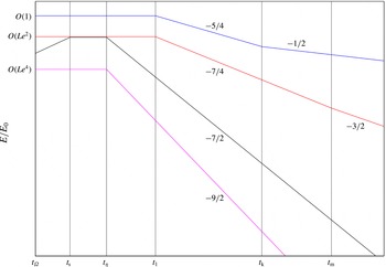
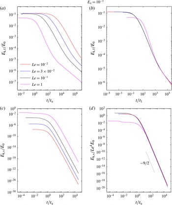
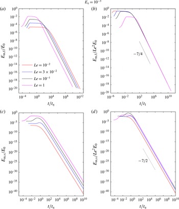
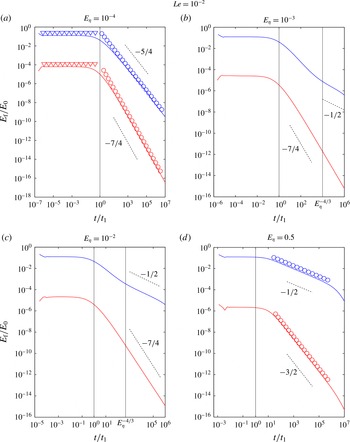
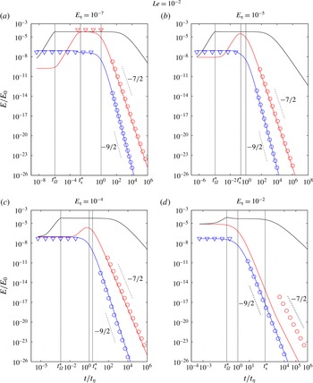
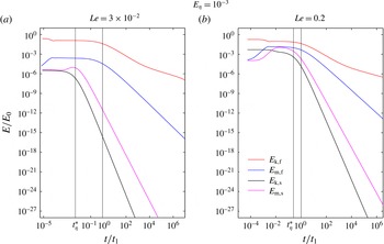
Figure 2 shows the evolution of kinetic and magnetic energies in the regime of strong rotation. As the slow MC waves decay much faster than the fast MC waves, the long-time decay of vortices is essentially controlled by the decay of the fast waves.
Decay of energies in the regime of strong rotation. The four lines represent the fast wave kinetic (blue), fast wave magnetic (red), slow wave kinetic (magenta) and slow wave magnetic (black) energies. The times
 $t_{\text{k}}$
and
 $t_{\text{m}}$
, defined in (3.64) and (3.67), mark the wave–diffusion transitions of the fast wave kinetic and magnetic energies. The time
 $t_{1}$
is defined in (3.18),
 $t_{\unicode[STIX]{x1D6FA}}$
is defined in (3.29),
 $t_{\unicode[STIX]{x1D702}}$
is defined in (3.40) and
 $t_{\text{s}}$
is defined in (3.49).

4 Weak rotation: Approximate analytical solutions
In this section, we consider the regime of weak rotation, where the Alfvén wave frequency
 $V_{A}k_{z}$
is much higher in magnitude than the inertial wave frequency
 $\unicode[STIX]{x1D6FA}k_{z}/k$
. It must be noted that the Rossby number
 $Ro\ll 1$
in this regime, so that the nonlinear inertial force is still negligible compared with the Coriolis force in the equation of motion.
In the inviscid limit, the relative orders of magnitude of the fundamental frequencies in the two phases of decay are given by the following inequalities:
-
(i)
$V_{A}k_{z}\gg \unicode[STIX]{x1D6FA}k_{z}/k\gg \unicode[STIX]{x1D702}k^{2}/2$
(wave-dominated phase); -
(ii)
$\unicode[STIX]{x1D702}k^{2}/2\gg V_{A}k_{z}\gg \unicode[STIX]{x1D6FA}k_{z}/k$
(diffusion-dominated phase).


We begin by obtaining approximations for the fast (
 $\unicode[STIX]{x1D706}_{1,2}$
) and slow (
 $\unicode[STIX]{x1D706}_{3,4}$
) MC wave frequencies in the two phases.
4.1 Frequency approximations in the wave-dominated phase
Noting that
 $V_{A}k_{z}$
is the dominant frequency in this phase, the fast MC wave frequency
 $\unicode[STIX]{x1D706}_{1}$
(appendix A) in the inviscid limit is rewritten in the form
 $$\begin{eqnarray}\unicode[STIX]{x1D706}_{1}=\frac{\unicode[STIX]{x1D6FA}k_{z}}{k}+\text{i}\frac{\unicode[STIX]{x1D702}k^{2}}{2}+V_{A}k_{z}\sqrt{1+\left(\frac{\unicode[STIX]{x1D6FA}}{V_{A}k}-\text{i}\frac{\unicode[STIX]{x1D702}k^{2}}{2V_{A}k_{z}}\right)^{2}}.\end{eqnarray}$$
Since
 $\unicode[STIX]{x1D702}k^{2}/2V_{A}k_{z}\ll \unicode[STIX]{x1D6FA}/V_{A}k\ll 1$
, further simplification gives
 $$\begin{eqnarray}\unicode[STIX]{x1D706}_{1}\approx \left(V_{A}k_{z}+\frac{\unicode[STIX]{x1D6FA}k_{z}}{k}\right)+\text{i}\left(\frac{\unicode[STIX]{x1D702}k^{2}}{2}-\frac{\unicode[STIX]{x1D6FA}\unicode[STIX]{x1D702}k}{2V_{A}}\right).\end{eqnarray}$$
In a similar way,
 $$\begin{eqnarray}\unicode[STIX]{x1D706}_{2}\approx -\left(V_{A}k_{z}+\frac{\unicode[STIX]{x1D6FA}k_{z}}{k}\right)+\text{i}\left(\frac{\unicode[STIX]{x1D702}k^{2}}{2}-\frac{\unicode[STIX]{x1D6FA}\unicode[STIX]{x1D702}k}{2V_{A}}\right).\end{eqnarray}$$
The slow MC wave frequency
 $\unicode[STIX]{x1D706}_{3}$
(appendix A) is rewritten in the form
 $$\begin{eqnarray}\unicode[STIX]{x1D706}_{3}=-\frac{\unicode[STIX]{x1D6FA}k_{z}}{k}+\text{i}\frac{\unicode[STIX]{x1D702}k^{2}}{2}+V_{A}k_{z}\sqrt{1+\left(\frac{\unicode[STIX]{x1D6FA}}{V_{A}k}+\text{i}\frac{\unicode[STIX]{x1D702}k^{2}}{2V_{A}k_{z}}\right)^{2}}\end{eqnarray}$$
and approximated by
 $$\begin{eqnarray}\unicode[STIX]{x1D706}_{3}\approx \left(V_{A}k_{z}-\frac{\unicode[STIX]{x1D6FA}k_{z}}{k}\right)+\text{i}\left(\frac{\unicode[STIX]{x1D702}k^{2}}{2}+\frac{\unicode[STIX]{x1D6FA}\unicode[STIX]{x1D702}k}{2V_{A}}\right).\end{eqnarray}$$
In a similar way,
 $$\begin{eqnarray}\unicode[STIX]{x1D706}_{4}\approx -\left(V_{A}k_{z}-\frac{\unicode[STIX]{x1D6FA}k_{z}}{k}\right)+\text{i}\left(\frac{\unicode[STIX]{x1D702}k^{2}}{2}+\frac{\unicode[STIX]{x1D6FA}\unicode[STIX]{x1D702}k}{2V_{A}}\right).\end{eqnarray}$$
4.2 Frequency approximations in the diffusion-dominated phase
Noting that
 $\unicode[STIX]{x1D702}k^{2}/2$
is the dominant frequency in this phase, the fast MC wave frequency
 $\unicode[STIX]{x1D706}_{1}$
is rewritten in the form
 $$\begin{eqnarray}\unicode[STIX]{x1D706}_{1}=\frac{\unicode[STIX]{x1D6FA}k_{z}}{k}+\text{i}\frac{\unicode[STIX]{x1D702}k^{2}}{2}+\frac{\unicode[STIX]{x1D702}k^{2}}{2}\sqrt{\left(\frac{2V_{A}k_{z}}{\unicode[STIX]{x1D702}k^{2}}\right)^{2}+\left(\frac{2\unicode[STIX]{x1D6FA}k_{z}}{\unicode[STIX]{x1D702}k^{3}}-\text{i}\right)^{2}}.\end{eqnarray}$$
Since
 $2\unicode[STIX]{x1D6FA}k_{z}/\unicode[STIX]{x1D702}k^{3}\ll 2V_{A}k_{z}/\unicode[STIX]{x1D702}k^{2}\ll 1$
, further simplification gives
 $$\begin{eqnarray}\unicode[STIX]{x1D706}_{1}\approx \frac{2\unicode[STIX]{x1D6FA}k_{z}}{k}+\text{i}\frac{k_{z}^{2}}{\unicode[STIX]{x1D70F}k^{2}}.\end{eqnarray}$$
In a similar way,
 $$\begin{eqnarray}\unicode[STIX]{x1D706}_{2}\approx -\frac{2\unicode[STIX]{x1D6FA}k_{z}}{k}+\text{i}\frac{k_{z}^{2}}{\unicode[STIX]{x1D70F}k^{2}}.\end{eqnarray}$$
The slow MC wave frequency
 $\unicode[STIX]{x1D706}_{3}$
is rewritten in the form
 $$\begin{eqnarray}\unicode[STIX]{x1D706}_{3}=-\frac{\unicode[STIX]{x1D6FA}k_{z}}{k}+\text{i}\frac{\unicode[STIX]{x1D702}k^{2}}{2}+\frac{\unicode[STIX]{x1D702}k^{2}}{2}\sqrt{\left(\frac{2V_{A}k_{z}}{\unicode[STIX]{x1D702}k^{2}}\right)^{2}+\left(\frac{2\unicode[STIX]{x1D6FA}k_{z}}{\unicode[STIX]{x1D702}k^{3}}+\text{i}\right)^{2}}\end{eqnarray}$$
and approximated by
 $$\begin{eqnarray}\unicode[STIX]{x1D706}_{3}\approx \frac{2\unicode[STIX]{x1D6FA}V_{A}^{2}k_{z}^{3}}{\unicode[STIX]{x1D702}^{2}k^{5}}+\text{i}\unicode[STIX]{x1D702}k^{2}.\end{eqnarray}$$
In a similar way,
 $$\begin{eqnarray}\unicode[STIX]{x1D706}_{4}\approx -\frac{2\unicode[STIX]{x1D6FA}V_{A}^{2}k_{z}^{3}}{\unicode[STIX]{x1D702}^{2}k^{5}}+\text{i}\unicode[STIX]{x1D702}k^{2}.\end{eqnarray}$$
The
 $\unicode[STIX]{x1D706}_{1,2}$
frequency approximations (4.8) and (4.9) are the same as those obtained in (3.12) and (3.13), implying that the diffusion-dominated quasistatic (
 $qs$
) phase (appendix A, equation (A 4) for
 $\unicode[STIX]{x1D708}=0$
) is common to the regimes of strong and weak rotation. The two modes that physically exist in the
 $qs$
phase are those of the fast wave,
 $\unicode[STIX]{x1D706}_{1,2}$
. The slow wave modes
 $\unicode[STIX]{x1D706}_{3,4}$
are not relevant to this phase as they represent isotropic decay.
4.3 Energy decay and wave–diffusion transition
We investigate the decay of kinetic and magnetic energies in the inviscid (
 $\unicode[STIX]{x1D708}=0$
) limit. Using the frequency approximations (4.8), (4.9), (4.11) and (4.12) as well as the inequality
 $V_{A}k_{z}\gg \unicode[STIX]{x1D6FA}k_{z}/k\gg \unicode[STIX]{x1D702}k^{2}/2$
for the wave-dominated phase, we obtain at leading order
 $$\begin{eqnarray}\displaystyle & \displaystyle \hat{u} _{\unicode[STIX]{x1D719},\text{f}}\approx \frac{\hat{u} _{\unicode[STIX]{x1D719}0}}{4}\exp (-\unicode[STIX]{x1D6FD}_{1}t)\left[\cos \unicode[STIX]{x1D6FC}_{1}t+\left(\frac{\unicode[STIX]{x1D702}k^{2}}{2V_{A}k_{z}}-\frac{9\unicode[STIX]{x1D6FA}\unicode[STIX]{x1D702}k}{4V_{A}^{2}k_{z}}\right)\sin \unicode[STIX]{x1D6FC}_{1}t\right], & \displaystyle\end{eqnarray}$$
 $$\begin{eqnarray}\displaystyle & \displaystyle \hat{u} _{\unicode[STIX]{x1D719},\text{s}}\approx \frac{\hat{u} _{\unicode[STIX]{x1D719}0}}{4}\exp (-\unicode[STIX]{x1D6FD}_{2}t)\left[\cos \unicode[STIX]{x1D6FC}_{2}t+\left(\frac{\unicode[STIX]{x1D702}k^{2}}{2V_{A}k_{z}}+\frac{9\unicode[STIX]{x1D6FA}\unicode[STIX]{x1D702}k}{4V_{A}^{2}k_{z}}\right)\sin \unicode[STIX]{x1D6FC}_{2}t\right], & \displaystyle\end{eqnarray}$$
 $$\begin{eqnarray}\displaystyle & \displaystyle \hat{b}_{\unicode[STIX]{x1D719},\text{f}}\approx \text{i}\sqrt{\unicode[STIX]{x1D707}\unicode[STIX]{x1D70C}}\frac{\hat{u} _{\unicode[STIX]{x1D719}0}}{4}\exp (-\unicode[STIX]{x1D6FD}_{1}t)\left[\sin \unicode[STIX]{x1D6FC}_{1}t+\left(\frac{3\unicode[STIX]{x1D702}\unicode[STIX]{x1D6FA}k}{4V_{A}^{2}k_{z}}\right)\cos \unicode[STIX]{x1D6FC}_{1}t\right], & \displaystyle\end{eqnarray}$$
 $$\begin{eqnarray}\displaystyle & \displaystyle \hat{b}_{\unicode[STIX]{x1D719},\text{s}}\approx \text{i}\sqrt{\unicode[STIX]{x1D707}\unicode[STIX]{x1D70C}}\frac{\hat{u} _{\unicode[STIX]{x1D719}0}}{4}\exp (-\unicode[STIX]{x1D6FD}_{2}t)\left[\sin \unicode[STIX]{x1D6FC}_{2}t+\left(\frac{3\unicode[STIX]{x1D702}\unicode[STIX]{x1D6FA}k}{4V_{A}^{2}k_{z}}\right)\cos \unicode[STIX]{x1D6FC}_{2}t\right], & \displaystyle\end{eqnarray}$$
where
 $$\begin{eqnarray}\unicode[STIX]{x1D6FC}_{1}=V_{A}k_{z}+\frac{\unicode[STIX]{x1D6FA}k_{z}}{k},\quad \unicode[STIX]{x1D6FD}_{1}=\frac{\unicode[STIX]{x1D702}k^{2}}{2}-\frac{\unicode[STIX]{x1D6FA}\unicode[STIX]{x1D702}k}{2V_{A}};\end{eqnarray}$$
 $$\begin{eqnarray}\unicode[STIX]{x1D6FC}_{2}=V_{A}k_{z}-\frac{\unicode[STIX]{x1D6FA}k_{z}}{k},\quad \unicode[STIX]{x1D6FD}_{2}=\frac{\unicode[STIX]{x1D702}k^{2}}{2}+\frac{\unicode[STIX]{x1D6FA}\unicode[STIX]{x1D702}k}{2V_{A}}.\end{eqnarray}$$
In the limit
 $V_{A}k/\unicode[STIX]{x1D6FA}\rightarrow \infty$
, equations (4.13)–(4.16) take the form
 $$\begin{eqnarray}\displaystyle & \displaystyle \hat{u} _{\unicode[STIX]{x1D719},\text{f}}=\hat{u} _{\unicode[STIX]{x1D719},\text{s}}\approx \frac{\hat{u} _{\unicode[STIX]{x1D719}0}}{4}\exp \left(-\frac{\unicode[STIX]{x1D702}k^{2}}{2}t\right)\left[\cos (V_{A}k_{z}t)+\frac{\unicode[STIX]{x1D702}k^{2}}{2V_{A}k_{z}}\sin (V_{A}k_{z}t)\right], & \displaystyle\end{eqnarray}$$
 $$\begin{eqnarray}\displaystyle & \displaystyle \hat{b}_{\unicode[STIX]{x1D719},\text{f}}=\hat{b}_{\unicode[STIX]{x1D719},\text{s}}\approx \text{i}\sqrt{\unicode[STIX]{x1D707}\unicode[STIX]{x1D70C}}\frac{\hat{u} _{\unicode[STIX]{x1D719}0}}{4}\exp \left(-\frac{\unicode[STIX]{x1D702}k^{2}}{2}t\right)\sin (V_{A}k_{z}t). & \displaystyle\end{eqnarray}$$
Using equation (2.8) for
 $\hat{u} _{\unicode[STIX]{x1D719}0}$
and Parseval’s theorem, the kinetic energy for times
 $t\gtrsim t_{\unicode[STIX]{x1D702}}$
is given by
 $$\begin{eqnarray}E_{\text{k}}\approx \frac{\unicode[STIX]{x03C0}\unicode[STIX]{x1D6FF}^{10}}{64}\int _{0}^{\infty }\int _{0}^{\infty }k_{s}^{3}\exp \left[-\left(\frac{k^{2}\unicode[STIX]{x1D6FF}^{2}}{2}+\unicode[STIX]{x1D702}k^{2}t\right)\right]\,\text{d}k_{s}\,\text{d}k_{z},\end{eqnarray}$$
which, by using the solutions for
 $I_{0}(a)$
and
 $I_{3}(a)$
(B 15, appendix B), gives
 $$\begin{eqnarray}E_{\text{k}}\approx \frac{\unicode[STIX]{x03C0}\unicode[STIX]{x1D6FF}^{10}}{256}\times \frac{1}{(\unicode[STIX]{x1D6FF}^{2}/2+\unicode[STIX]{x1D702}t)^{2}}\times \sqrt{\frac{\unicode[STIX]{x03C0}}{\unicode[STIX]{x1D6FF}^{2}/2+\unicode[STIX]{x1D702}t}},\end{eqnarray}$$
and, for
 $t\gg t_{\unicode[STIX]{x1D702}}$
,
 $$\begin{eqnarray}E_{\text{k}}\approx \frac{25\sqrt{5}\unicode[STIX]{x03C0}^{3/2}\unicode[STIX]{x1D6FF}^{5}}{256}\left(\frac{t}{t_{\unicode[STIX]{x1D702}}}\right)^{-5/2}.\end{eqnarray}$$
A similar analysis gives the magnetic energy
 $E_{\text{m}}=E_{\text{k}}$
. The decay law in (4.23) was obtained for the damped (Alfvén) wave phase in non-rotating MHD turbulence at
 $Rm\ll 1$
and
 $N\gg 1$
(Moffatt Reference Moffatt1967).
In the diffusion-dominated phase (
 $\unicode[STIX]{x1D702}k^{2}/2\gg V_{A}k_{z}\gg \unicode[STIX]{x1D6FA}k_{z}/k$
), the energies follow the decay laws
 $$\begin{eqnarray}E_{\text{k}}/E_{0}\sim (t/\unicode[STIX]{x1D70F})^{-1/2},\quad E_{\text{m}}/E_{0}\sim S^{2}(t/\unicode[STIX]{x1D70F})^{-3/2},\end{eqnarray}$$
as in (3.60) and (3.61) respectively.
From (4.23) and (4.24), the time scale for wave–diffusion transition of
 $E_{\text{k}}$
is obtained from the condition
 $$\begin{eqnarray}\left(\frac{t}{t_{\unicode[STIX]{x1D702}}}\right)^{-5/2}\sim \left(\frac{t}{\unicode[STIX]{x1D70F}}\right)^{-1/2},\end{eqnarray}$$
which gives
 $$\begin{eqnarray}t=t_{\text{k}}\sim S^{1/2}t_{\unicode[STIX]{x1D702}}.\end{eqnarray}$$
The time scale for wave–diffusion transition of
 $E_{\text{m}}$
is obtained from the condition
 $$\begin{eqnarray}\left(\frac{t}{t_{\unicode[STIX]{x1D702}}}\right)^{-5/2}\sim S^{2}\left(\frac{t}{\unicode[STIX]{x1D70F}}\right)^{-3/2},\end{eqnarray}$$
which gives
 $$\begin{eqnarray}t=t_{\text{m}}\sim St_{\unicode[STIX]{x1D702}}.\end{eqnarray}$$
5 Computed general solution
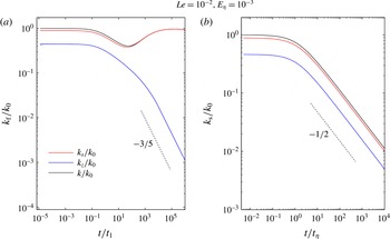
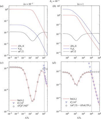
The general solution of our initial value problem, given by (2.2) and (2.3), is computed. The values of
 $\hat{u} _{\unicode[STIX]{x1D719}}$
and
 $\hat{b}_{\unicode[STIX]{x1D719}}$
and their respective energies are calculated at discrete time points
 $t$
, each decade in time being covered by 30 points. To resolve the fast wave velocity,
 $2\times 10^{5}$
spectral points are used in
 $k_{s}$
and
 $k_{z}$
, whereas the fast wave magnetic field and the slow waves are adequately resolved by
 $2\times 10^{4}$
points. Because of progressive magnetic diffusion, the truncation values of
 $k_{s}$
and
 $k_{z}$
can be decreased in time, which means that the computations are well resolved at large times. The initial truncation value for both wavenumbers is set to 50, in view of the mean initial wavenumbers
 $k_{s0}=8$
and
 $k_{z0}=4$
for the flow given by (2.1) with the chosen initial length scale
 $\unicode[STIX]{x1D6FF}=1/4$
. The kinetic and magnetic energies are calculated from the exact velocity and induced field transforms by Parseval’s theorem (see, e.g., (3.19) and (3.30)), where the upper limits of the integrals are the truncation values of
 $k_{s}$
and
 $k_{z}$
. The computed energies are then compared with their analytical approximations derived from the leading-order inviscid solutions of the transforms.
Viscous diffusion is kept small by choosing a small magnetic Prandtl number,
 $Pm=10^{-10}$
. The magnetic Reynolds number
 $Rm$
based on the peak value of the initial velocity
 $u_{\unicode[STIX]{x1D719}0}$
and the length scale
 $\unicode[STIX]{x1D6FF}$
is
 $10^{-2}$
. The mean magnetic field intensity
 $B_{0}$
and the background rotation rate
 $\unicode[STIX]{x1D6FA}$
are chosen such that the Lehnert number
 $Le=V_{A}/2\unicode[STIX]{x1D6FA}\unicode[STIX]{x1D6FF}$
varies in the range
 $10^{-2}{-}1$
, representing the regimes of strong as well as relatively weak background rotation. Although
 $Le$
based on the length scale of the Earth’s outer core (
 ${\sim}10^{3}~\text{km}$
) can lie in the range
 $3\times 10^{-5}$
–
 $5\times 10^{-4}$
(Jault Reference Jault2008; Gillet, Schaeffer & Jault Reference Gillet, Schaeffer and Jault2011), for the small-scale structures of
 $Rm\sim 1$
or less considered in this study,
 $Le\sim 10^{-2}$
represents the regime of strong rotation. The value of
 $E_{\unicode[STIX]{x1D702}}$
(defined in (3.65)) determines whether the solution is wave-dominated (
 $E_{\unicode[STIX]{x1D702}}\ll 1$
) or strongly affected by magnetic diffusion (
 $E_{\unicode[STIX]{x1D702}}\sim 1$
) initially. The Rossby number
 $Ro=E_{\unicode[STIX]{x1D702}}Rm\ll 1$
throughout this study.
To compute the frequencies, the mean values of the wavenumbers for the velocity field are first calculated through ratios of
 $L^{2}$
norms,
 $$\begin{eqnarray}\overline{k}_{z}=\frac{\Vert k_{z}\hat{u} _{\unicode[STIX]{x1D719}}\Vert }{\Vert \hat{u} _{\unicode[STIX]{x1D719}}\Vert },\quad \overline{k}=\frac{\Vert k\hat{u} _{\unicode[STIX]{x1D719}}\Vert }{\Vert \hat{u} _{\unicode[STIX]{x1D719}}\Vert }.\end{eqnarray}$$
Computed values of the wavenumbers
 $k_{z}$
,
 $k_{s}$
and
 $k$
normalized by the initial wavenumber
 $k_{0}$
for (a) the fast MC wave velocity (subscript f) and (b) the slow MC wave velocity (subscript s). The time axes are normalized by the respective decay time scales,
 $t_{1}$
and
 $t_{\unicode[STIX]{x1D702}}$
.

Plots of the
 $z$
,
 $s$
and resultant wavenumbers shown individually for the fast and slow MC wave components (figure 3
a,b) reveal a basic difference between the two waves. For the fast wave,
 $k_{z}$
alone decreases progressively in time, whereas
 $k_{s}$
and
 $k$
do not change much (panel a). In contrast, the slow wave wavenumbers decrease together in time (panel b). (The slopes of decay for the two waves are also measured.) The inference is that the fast wave undergoes strongly anisotropic magnetic diffusion whereas the slow wave diffusion is isotropic.
Computed frequencies for the fast wave solution
 $\hat{u} _{\unicode[STIX]{x1D719},\text{f}}$
in the regimes of strong (
 $Le=10^{-2}$
) and relatively weak (
 $Le=1$
) rotation. (a,b) The fundamental frequencies of the inertial wave (
 $\unicode[STIX]{x1D6FA}k_{z}/k$
), Alfvén wave (
 $V_{A}k_{z}$
) and magnetic diffusion (
 $\unicode[STIX]{x1D702}k^{2}/2$
). (c,d) A comparison of the imaginary part of the frequency
 $\unicode[STIX]{x1D706}_{1}$
with its approximations in the wave and diffusive phases of decay.

Computed frequencies for the slow wave solution
 $\hat{u} _{\unicode[STIX]{x1D719},\text{s}}$
in the regimes of strong (
 $Le=10^{-2}$
) and relatively weak (
 $Le=1$
) rotation. (a,b) The fundamental frequencies of the inertial wave (
 $\unicode[STIX]{x1D6FA}k_{z}/k$
), Alfvén wave (
 $V_{A}k_{z}$
) and magnetic diffusion (
 $\unicode[STIX]{x1D702}k^{2}/2$
). (c,d) A comparison of the imaginary part of the frequency
 $\unicode[STIX]{x1D706}_{3}$
with its approximations.

Figures 4 and 5 present the computed frequencies of the fast and slow wave components,
 $\hat{u} _{\unicode[STIX]{x1D719},\text{f}}$
and
 $\hat{u} _{\unicode[STIX]{x1D719},\text{s}}$
, separately. We choose
 $E_{\unicode[STIX]{x1D702}}=10^{-3}$
, which is sufficiently small for wave motion to be dominant initially. For the fast wave (figure 4), the three fundamental frequencies shown in (a) and (b) follow their anticipated orders of magnitude. The strongly rotating regime (
 $Le=10^{-2}$
) has
 $\unicode[STIX]{x1D6FA}k_{z}/k>V_{A}k_{z}$
throughout, and
 $\unicode[STIX]{x1D702}k^{2}/2$
becomes the dominant frequency at
 $t\approx 10^{5}t_{1}$
(marked by the thin vertical line). The weakly rotating regime (
 $Le=1$
) has
 $V_{A}k_{z}>\unicode[STIX]{x1D6FA}k_{z}/k$
throughout, with
 $\unicode[STIX]{x1D702}k^{2}/2$
eventually gaining the upper hand at
 $t\approx 10^{6}t_{1}$
. The wave–diffusion transition is thus evident in both regimes. The interesting point, however, is that the magnitude of Lehnert’s parameter
 $\unicode[STIX]{x1D701}$
(1.1) has fallen well below unity at the transition in figure 4(a), whereas
 $\unicode[STIX]{x1D701}=1$
at the transition in figure 4(b). Since
 $t_{1}$
varies as
 $1/Le^{2}$
, the wave–diffusion transition for strong rotation occurs much later than that for weak rotation.
In figure 4(c,d), the computed imaginary part of the fast wave frequency
 $\unicode[STIX]{x1D706}_{1}$
is compared with the frequency approximations in the wave-dominated and diffusion-dominated phases of decay. For strong rotation (
 $Le=10^{-2}$
),
 $\text{Im}\{\unicode[STIX]{x1D706}_{1}\}$
matches closely with
 $\unicode[STIX]{x1D702}V_{A}^{2}k^{4}/4\unicode[STIX]{x1D6FA}^{2}$
(see (3.5)) only in the wave-dominated phase, and with
 $k_{z}^{2}/\unicode[STIX]{x1D70F}k^{2}$
(see (3.12)) only in the diffusion-dominated phase. For relatively weak rotation (
 $Le=1$
),
 $\text{Im}\{\unicode[STIX]{x1D706}_{1}\}$
matches closely with
 $(\unicode[STIX]{x1D702}k^{2}/2-\unicode[STIX]{x1D6FA}\unicode[STIX]{x1D702}k/2V_{A})$
(see (4.2)) only in the wave-dominated phase, and with
 $k_{z}^{2}/\unicode[STIX]{x1D70F}k^{2}$
(see (4.8)) only in the diffusion-dominated phase. In short, the frequency approximations in the two phases of decay faithfully reproduce the actual frequency of the wave.
Turning to the computed slow wave frequencies (figure 5), we find that the diffusion frequency
 $\unicode[STIX]{x1D702}k^{2}/2$
never exceeds
 $\unicode[STIX]{x1D6FA}k_{z}/k$
or
 $V_{A}k_{z}$
, which indicates that the slow wave decays independently of the wave–diffusion transition of the fast wave. From figure 5(c), we note that
 $\text{Im}\{\unicode[STIX]{x1D706}_{3}\}$
matches closely with
 $\unicode[STIX]{x1D702}k^{2}$
(see (3.9), (3.15)) throughout the decay. For relatively weak rotation (
 $Le=1$
),
 $V_{A}k_{z}$
is initially greater than
 $\unicode[STIX]{x1D6FA}k_{z}/k$
(figure 5
b), during which period
 $\text{Im}\{\unicode[STIX]{x1D706}_{3}\}$
is well approximated by
 $(\unicode[STIX]{x1D702}k^{2}/2+\unicode[STIX]{x1D6FA}\unicode[STIX]{x1D702}k/2V_{A})$
(see (4.5)). Subsequently, however,
 $\unicode[STIX]{x1D6FA}k_{z}/k$
becomes dominant, upon which
 $\text{Im}\{\unicode[STIX]{x1D706}_{2}\}$
is approximated by
 $\unicode[STIX]{x1D702}k^{2}$
, as in the regime of strong rotation (figure 5
d).
Contour plots at three different times of the fast MC wave velocity spectrum
 $\hat{u} _{\unicode[STIX]{x1D719},\text{f}}$
for (a–c) the regime of strong rotation (
 $Le=10^{-2}$
) and (d–f) the regime of relatively weak rotation (
 $Le=1$
).

Contour plots at three different times of the slow MC wave velocity spectrum
 $\hat{u} _{\unicode[STIX]{x1D719},\text{s}}$
in the regime of strong rotation (
 $Le=10^{-2}$
).

The velocity spectra of the fast and slow MC waves (figures 6 and 7) show that their decay patterns are fundamentally different. In strong rotation (
 $Le=10^{-2}$
), the fast wave spectrum develops a very fine banded structure within
 $t\sim 10t_{1}$
, visualized only by significantly reducing the
 $k_{z}$
-axis range (figure 6
b,c). For relatively weak rotation (
 $Le=1$
), the fine structure develops only at large times, so the effect of anisotropic magnetic diffusion is noticeable. The initial spectrum (figure 6
d) evolves into a conical section where all of the energy is concentrated in the neighbourhood of the
 $k_{s}$
-axis and ohmic dissipation is dominant near the
 $k_{z}$
-axis (e.g. Alemany et al.
Reference Alemany, Moreau, Sulem and Frisch1979). The half-angle of the cone,
 $\unicode[STIX]{x1D703}=\cos ^{-1}(k_{z}/k)$
, increases with time (figure 6
e,f), indicating progressive increase of flow anisotropy. The slow MC wave spectrum, in contrast, shrinks isotropically in time (figure 7
a–c) because its decay factor
 $\text{e}^{-\unicode[STIX]{x1D702}k^{2}t}$
is independent of the angle
 $\unicode[STIX]{x1D703}$
(see (3.39)).
Comparison of the toroidal and poloidal kinetic (subscript k) and magnetic (subscript m) energies for two values of
 $Le$
. The toroidal energies are shown with solid lines and the poloidal energies with symbols.

Since the poloidal
 $(s,z)$
components of the velocity and induced magnetic field may be obtained in a form similar to (2.2) and (2.3), their energies are computed and compared with the toroidal energies (figure 8). Except for an early phase of evolution, the background rotation equalizes the poloidal and toroidal energies for both values of
 $Le$
. Therefore, the laws derived for the evolution of toroidal energy (§§ 3 and 4) also hold for the total energy of the system. The brief equipartition between
 $E_{\text{k}}$
and
 $E_{\text{m}}$
noted for
 $Le=1$
would last longer for
 $Le>1$
(weaker rotation).
Evolution of kinetic energy of the fast (a,b) and slow (c,d) MC wave components for four values of
 $Le$
. The colour codes for all panels are given in (a).

Figure 9 confirms the scalings obtained for the kinetic energy. As in previous figures, we set
 $E_{\unicode[STIX]{x1D702}}=10^{-3}$
, giving initial wave dominance. With time scaled with respect to
 $t_{1}$
, the computed fast wave energies at different values of
 $Le$
(figure 9
a) collapse to a single curve, with the exception of the case
 $Le=1$
which has the weakest rotation (figure 9
b). A lower value of
 $E_{\unicode[STIX]{x1D702}}$
is required to see a wave phase decay law spanning several decades (see figure 11
a below). As the energy decay is not rotation-dependent in the diffusion-dominated phase, the curve for
 $Le=1$
merges with the other curves in this phase. The slow wave kinetic energy is self-similar when scaled by
 $Le^{4}$
, and follows the
 $(t/t_{\unicode[STIX]{x1D702}})^{-9/2}$
decay law (see (3.70) and figure 9
d), except for the case
 $Le=1$
which does not have the
 $O(Le^{4})$
scaling for
 $t<t_{\unicode[STIX]{x1D702}}$
. Figure 10 gives the evolution of magnetic energy for
 $E_{\unicode[STIX]{x1D702}}=10^{-3}$
and different
 $Le$
. The fast wave magnetic energy
 $E_{\text{m},\text{f}}$
scaled by
 $Le^{2}$
decays as
 $(t/t_{1})^{-7/4}$
in self-similar fashion (see (3.69) and figure 10
b) except for the case
 $Le=1$
which does not have the
 $O(Le^{2})$
scaling for
 $t<t_{\unicode[STIX]{x1D702}}$
. The slow wave magnetic energy
 $E_{\text{m},\text{s}}$
scaled by
 $Le^{2}$
follows a robust
 $(t/t_{\unicode[STIX]{x1D702}})^{-7/2}$
decay (see (3.71) and figure 10
d); that having been said, the self-similarity is not exact because the field evolution in the initial transient is different in each case (see also figure 12).
Evolution of magnetic energy of the fast (a,b) and slow (c,d) MC wave components for four values of
 $Le$
. The colour codes for all panels are given in (a).

The computed kinetic (blue line) and magnetic (red line) energies of the fast (f) MC wave, with their approximate analytical estimates shown with symbols. In (a), the blue triangles give the initial energy ratio
 $1/4$
(3.20), the blue circles are obtained from (3.27), the red triangles from (3.32) and the red circles from (3.38). In (d), the blue circles are obtained from (3.60) and the red circles from (3.61).

The computed kinetic (blue line) and magnetic (red line) energies of the slow (s) MC wave, with their approximate analytical estimates shown with symbols. The fast wave magnetic energy (black line) is provided for comparison. The blue triangles are obtained from (3.43), the blue circles from (3.47), the red triangles from (3.51) and the red circles from (3.55). The dimensionless times marked on the horizontal axes are
 $t_{\unicode[STIX]{x1D6FA}}^{\ast }=t_{\unicode[STIX]{x1D6FA}}/t_{\unicode[STIX]{x1D702}}$
and
 $t_{\text{s}}^{\ast }=t_{\text{s}}/t_{\unicode[STIX]{x1D702}}$
, where
 $t_{\unicode[STIX]{x1D6FA}}$
is defined in (3.29) and
 $t_{\text{s}}$
is defined in (3.49).

Figure 11 compares the computed kinetic and magnetic energies of the fast MC wave with their approximate analytical solutions. Because it is computationally difficult to capture both the wave-dominated phase and the subsequent diffusion-dominated phase in one calculation, separate calculations that focus on each phase as well as the wave–diffusion transition are performed by taking different values of
 $E_{\unicode[STIX]{x1D702}}$
. A sufficiently low value of
 $E_{\unicode[STIX]{x1D702}}$
(
 $10^{-4}$
) is required to see the
 ${\sim}t^{-5/4}$
wave phase decay of the kinetic energy that begins at
 $t\sim t_{1}$
(figure 11
a). Because of finite diffusion, this decay is not clearly visible in figure 11(b) or in figure 9(b), where
 $E_{\unicode[STIX]{x1D702}}=10^{-3}$
is taken. However, this run captures the wave–diffusion transition occurring at
 $t_{\text{k}}\approx 10^{4}t_{1}$
(i.e.
 ${\sim}E_{\unicode[STIX]{x1D702}}^{-4/3}t_{1}$
). As
 $E_{\unicode[STIX]{x1D702}}$
is increased, the diffusive phase lengthens at the expense of the wave phase, revealing the
 ${\sim}t^{-1/2}$
decay for
 $E_{\text{k},\text{f}}$
(figure 11
c). For
 $E_{\unicode[STIX]{x1D702}}=0.5$
, the evolution is entirely diffusion-dominated (figure 11
d). The fast wave magnetic energy
 $E_{\text{m},\text{f}}$
normalized by
 $E_{0}$
follows the
 $O(Le^{2})$
scaling in (3.32) for
 $t\ll t_{1}$
and the
 ${\sim}t^{-7/4}$
scaling in (3.38) for
 $t\gg t_{1}$
(figure 11
a). However, no wave–diffusion transition is noted for
 $E_{\unicode[STIX]{x1D702}}=10^{-4}$
–
 $10^{-2}$
. By increasing
 $E_{\unicode[STIX]{x1D702}}$
to 0.5, the diffusion-dominated
 ${\sim}t^{-3/2}$
decay for
 $E_{\text{m},\text{f}}$
is recovered (figure 11
d).
Figure 12 compares the computed kinetic and magnetic energies of the slow MC wave with their approximate analytical solutions. The fast wave magnetic energy, which develops on the time scale
 $t_{\unicode[STIX]{x1D6FA}}$
, is given for comparison. In all cases, the kinetic energy
 $E_{\text{k},\text{s}}$
normalized by
 $E_{0}$
closely follows the constant
 $O(Le^{4})$
scaling in (3.43) for
 $t\ll t_{\unicode[STIX]{x1D702}}$
and the
 ${\sim}t^{-9/2}$
scaling in (3.47) for
 $t\gg t_{\unicode[STIX]{x1D702}}$
. For
 $E_{\unicode[STIX]{x1D702}}=10^{-7}$
(figure 12
a), the slow wave time scale
 $t_{\text{s}}$
is sufficiently smaller than the diffusion time scale
 $t_{\unicode[STIX]{x1D702}}$
so that the magnetic energy
 $E_{\text{m},\text{s}}$
normalized by
 $E_{0}$
follows the
 $O(Le^{2})$
scaling (3.51) for the period
 $t_{\text{s}}<t<t_{\unicode[STIX]{x1D702}}$
. The magnetic energies of the slow and fast waves are equal during this period, in line with the theory for strong rotation (figure 2). Increase of
 $E_{\unicode[STIX]{x1D702}}$
causes progressive decrease of
 $E_{\text{m},\text{s}}$
relative to
 $E_{\text{m},\text{f}}$
due to enhanced diffusion. The computed value of
 $E_{\text{m},\text{s}}$
closely follows the
 ${\sim}t^{-7/2}$
scaling in (3.55) for
 $t\gg t_{\unicode[STIX]{x1D702}}$
, except for the case
 $E_{\unicode[STIX]{x1D702}}=10^{-2}$
(figure 12
d), where the computed value departs appreciably from theory. Here,
 $t_{\text{s}}\gg t_{\unicode[STIX]{x1D702}}$
, so that the Elsasser number
 $\unicode[STIX]{x1D6EC}\sim t_{\unicode[STIX]{x1D702}}/t_{\text{s}}$
is small. (More precisely, the Elsasser number for this case is
 $\unicode[STIX]{x1D6EC}=Le^{2}/E_{\unicode[STIX]{x1D702}}=10^{-2}$
.) In this regime, the slow magnetic modes are known to take the form of quasi-free-decay (QFD) magnetic modes (Schmitt Reference Schmitt2012; Canet, Finlay & Fournier Reference Canet, Finlay and Fournier2014). These modes are, however, not thought to be important for the Earth’s core, where the Elsasser number is much higher.
Contour plots of the toroidal velocity
 $u_{\unicode[STIX]{x1D719}}$
in the region
 $z>0$
at different times (in units of the magnetic diffusion time) for the parameters shown.

Contour plots of the toroidal velocity
 $u_{\unicode[STIX]{x1D719}}$
in the region
 $z>0$
at different times (in units of the magnetic diffusion time) for the parameters shown. The region where the slow MC wave is present in (a–c) is shown magnified in (d–f).

Contour plots of the toroidal velocity
 $u_{\unicode[STIX]{x1D719}}$
in the region
 $z>0$
at different times (in units of the magnetic diffusion time) for the parameters shown. In units of the Alfvén wave travel time
 $t_{A}$
, the respective times are (a)
 $2t_{A}$
, (b)
 $10t_{A}$
, (c)
 $50t_{A}$
, (d)
 $100t_{A}$
, (e)
 $500t_{A}$
and (f)
 $2000t_{A}$
.

Figures 13–15 show the evolution of the blob of fluid whose initial form is given by (2.1). The wave-dominated phase is in focus, wherein the magnetic diffusion frequency is kept small by the choice of a low magnetic Ekman number,
 $E_{\unicode[STIX]{x1D702}}=10^{-3}$
. Three values of the Lehnert number
 $Le$
are considered,
 $10^{-2}$
,
 $0.2$
and
 $1$
. In the strongly rotating regime of
 $Le=10^{-2}$
(figure 13), the solution is dominated by the fast MC wave, the behaviour of which is similar to that of the classical linear inertial wave in a non-magnetic system that propagates along the rotation axis (compare the
 $z$
-axis limits in figure 13). The slow MC wave does not show up in the contour plots because its velocity is very small in this regime. For
 $Le=0.2$
(figure 14), the slow MC wave appears, trailing the fast wave at small times. However, as shown separately in figure 14(d–f), the slow wave is damped rapidly, and would eventually fade away in the total solution. The effect of magnetic diffusion is already visible in the strands that connect the fast and slow wave components (figure 14
b). For
 $Le=1$
, the initial disturbance evolves as a diffused Alfvén wave (figure 15
a) and subsequently splits to form a fast wave and a slow wave component which are comparable in strength until
 $t\approx 0.5t_{\unicode[STIX]{x1D702}}$
(figure 15
b–e). Apart from the diffusion strands that connect the wave packets, the notable feature of this solution is that both the fast and the slow waves travel together along
 $z$
as a ‘unified’ wave at the Alfvén speed until the slow wave undergoes diffusion. This is evident from tracking the midpoint of the unified wave, which propagates as
 $z/\unicode[STIX]{x1D6FF}=t/t_{A}$
,
 $t_{A}$
being the Alfvén wave travel time. It is expected that with rotation tending to zero, the fast and slow wave solutions of equal magnitude would merge and tend to the non-dispersive damped Alfvén wave solution (see § 4.3).
It has been proposed that Alfvén waves form in rotating MHD turbulence in the limit
 $V_{A}k/\unicode[STIX]{x1D6FA}\rightarrow \infty$
, where
 $V_{A}/\unicode[STIX]{x1D6FA}$
is interpreted as a magnetoinertial length (Galtier Reference Galtier2014). While our study confirms that Alfvén waves are generated in this regime of weak rotation given by
 $V_{A}k_{z}\gg \unicode[STIX]{x1D6FA}k_{z}/k$
, we find that a magnetically damped system that initially produces Alfvén waves because of relatively weak rotation can subsequently give rise to fast and slow MC waves. A recent study of a forced undamped system where the magnetic field was orthogonal to the rotation axis (Bardsley & Davidson Reference Bardsley and Davidson2016) showed columnar structures propagating as Alfvén waves along the field lines in a regime that corresponds to that of weak rotation in this paper. If the wavenumber orthogonal to
 $\unicode[STIX]{x1D734}$
is much larger than the wavenumber parallel to it, a regime of weak rotation that supports Alfvén waves may be obtained for
 $Le\ll 1$
; that is, for a field strength much lower than that obtained in this study. Analysis of a forced damped system would help in estimating the smallest length scale that can support Alfvén waves in the Earth’s core in the face of magnetic diffusion.
6 Discussion
This study examines the long-time damping of an isolated flow structure subject to background rotation and a uniform coaxial magnetic field. The system obeys the conditions of
 $Rm\ll 1$
,
 $Ro\ll 1$
and
 $N\gg 1$
. In the regime of strong rotation, where
 $\unicode[STIX]{x1D6FA}k_{z}/k\gg V_{A}k_{z}\gg \unicode[STIX]{x1D702}k^{2}/2$
, the decay laws for the fast MC waves,
 $E_{\text{k},\text{f}}/E_{0}\sim (t/t_{1})^{-5/4}$
and
 $E_{\text{m},\text{f}}/E_{0}\sim Le^{2}(t/t_{1})^{-7/4}$
, determine the damping of the system. The slow MC waves decay far more rapidly as
 $E_{\text{k},\text{s}}/E_{0}\sim Le^{4}(t/t_{\unicode[STIX]{x1D702}})^{-9/2}$
and
 $E_{\text{m},\text{s}}/E_{0}\sim Le^{2}(t/t_{\unicode[STIX]{x1D702}})^{-7/2}$
. In the regime of weak rotation, where
 $V_{A}k_{z}\gg \unicode[STIX]{x1D6FA}k_{z}/k\gg \unicode[STIX]{x1D702}k^{2}/2$
, the decay laws for damped Alfvén waves in non-rotating MHD turbulence,
 $E_{\text{k}}/E_{0}=E_{\text{m}}/E_{0}\sim (t/t_{\unicode[STIX]{x1D702}})^{-5/2}$
, are recovered. In either regime, the diffusion-dominated phase follows the well-known decay laws
 $E_{\text{k}}/E_{0}\sim (t/\unicode[STIX]{x1D70F})^{-1/2}$
and
 $E_{\text{m}}/E_{0}\sim S^{2}(t/\unicode[STIX]{x1D70F})^{-3/2}$
for
 $qs$
MHD turbulence at
 $N\gg 1$
. These results indicate that the laws derived for an isolated vortex as the initial condition are applicable to freely decaying MHD turbulence originating from any velocity field. It is further known from laboratory experiments that the kinetic energy of a localized turbulent flow initiated by an electric current pulse decays as
 ${\sim}t^{-1/2}$
in the linear
 $qs$
phase (Sreenivasan & Alboussière Reference Sreenivasan and Alboussière2002), signifying that the energy decay is unaffected by the nature of the initial condition. In a strongly rotating system, where
 $E_{\unicode[STIX]{x1D702}}\ll 1$
, the time scale for the passage of the fast wave kinetic energy to the diffusion-dominated phase,
 $t_{\text{k}}\sim E_{\unicode[STIX]{x1D702}}^{-4/3}t_{1}$
, can be so large that the MHD turbulence would remain in the damped wave phase for a considerable period of time.
Since numerical simulations of the geodynamo (§ 1) suggest that rapid rotation forces convection to operate in small scales even in the presence of the magnetic field, it is essential to know whether scales of
 $Rm\sim 1$
or less can support fast and slow MC waves in the Earth’s core. Although length scales at which the Lundquist number
 $S\sim 1$
can have
 $Rm\ll 1$
(Nataf & Schaeffer Reference Nataf, Schaeffer and Olson2015), the longevity of these scales is determined by their wave–diffusion transition time scale. Because the frequency at which energy is injected through blobs of light elements near the inner core boundary is likely to be small compared with the frequency of the fast MC waves, analysis of a freely decaying MHD system provides some insight into the evolution of small scales in the core. Scales of
 $\unicode[STIX]{x1D6FF}\approx 2$
km give
 $Rm\approx 1$
and
 $E_{\unicode[STIX]{x1D702}}\approx 1.7\times 10^{-3}$
, by assuming
 $u=5\times 10^{-4}~\text{m}~\text{s}^{-1}$
(Starchenko & Jones Reference Starchenko and Jones2002) and
 $\unicode[STIX]{x1D702}=1~\text{m}^{2}~\text{s}^{-1}$
. For an average field strength
 $B_{0}=2~\text{mT}$
, the interaction parameter
 $N\approx 1270$
and the Lehnert number
 $Le\approx 6\times 10^{-2}$
, which can generate fast MC waves. The damping of the fast waves begins on the time scale
 $t_{1}\sim 4\unicode[STIX]{x1D6FA}^{2}\unicode[STIX]{x1D6FF}^{4}/\unicode[STIX]{x1D702}V_{A}^{2}$
(
 ${\sim}30$
years), and the wave–diffusion transition time scale for the kinetic energy is
 $t_{\text{k}}\sim 10^{5}$
years. (The onset of viscous diffusion occurs at
 $t_{\unicode[STIX]{x1D708}}\sim 10^{5}$
years, assuming
 $Pm\sim 10^{-6}$
for the core.) As the forcing from buoyancy cannot advance this time scale, turbulence at
 $Rm\sim 1$
would be in a state of perpetual damped wave motion, without ever seeing the diffusion-dominated
 $qs$
phase. In the absence of background rotation, small scales of
 $\unicode[STIX]{x1D6FF}\approx 2~\text{km}$
would have entered the diffusive phase on the time scale
 $S^{1/2}t_{\unicode[STIX]{x1D702}}\sim 275$
days, several orders of magnitude shorter than the wave–diffusion transition time with rotation.
The computed kinetic and magnetic energies of the fast and slow MC waves for a fixed
 $E_{\unicode[STIX]{x1D702}}$
and two values of
 $Le$
. The thin vertical lines show the onset of decay of the slow waves (
 $t=t_{\unicode[STIX]{x1D702}}$
) and the fast waves (
 $t=t_{1}$
). The colour codes given in (b) apply to both panels.

An important issue is the value of
 $Le$
that would support slow MC waves in core turbulence initiated by the injection of isolated blobs. In the regime of strong rotation, the kinetic energy of the slow wave
 $E_{\text{k},\text{s}}$
scales as
 $Le^{4}E_{0}$
for
 $t\ll t_{\unicode[STIX]{x1D702}}$
, whereas its magnetic energy
 $E_{\text{m},\text{s}}$
scales as
 $Le^{2}E_{0}$
for
 $t_{\text{s}}\ll t\ll t_{\unicode[STIX]{x1D702}}$
(figure 2). The induced magnetic field is thus far more efficient than the velocity in supporting slow MC waves for
 $Le\ll 1$
. Numerical experiments at
 $Le=10^{-2}$
show that
 $E_{\unicode[STIX]{x1D702}}$
must be less than
 $10^{-5}$
for
 $E_{\text{m},\text{s}}$
to be comparable to
 $E_{\text{m},\text{f}}$
in the early stages of evolution (see figure 12
a,b). It is therefore apparent that small-scale structures for which
 $E_{\unicode[STIX]{x1D702}}\sim 10^{-3}$
would require a higher
 $Le$
to support slow MC waves. The relative magnitudes of the slow and fast wave energies, shown in figure 16 for
 $E_{\unicode[STIX]{x1D702}}=10^{-3}$
and two values of
 $Le$
, support this line of reasoning. The case
 $Le=3\times 10^{-2}$
gives
 $E_{\text{m},\text{s}}\sim E_{\text{k},\text{s}}$
for
 $t<t_{\unicode[STIX]{x1D702}}$
, while
 $E_{\text{m},\text{f}}$
is substantially higher in magnitude. The case
 $Le=0.2$
, on the other hand, gives
 $E_{\text{m},\text{s}}\sim E_{\text{m},\text{f}}$
for
 $t<t_{\unicode[STIX]{x1D702}}$
, suggesting that both slow and fast waves are generated simultaneously before their diffusion sets in at times
 $t_{\unicode[STIX]{x1D702}}$
and
 $t_{1}$
respectively. Furthermore,
 $E_{\text{k},\text{s}}$
is much closer to
 $E_{\text{k},\text{f}}$
for
 $Le=0.2$
than for
 $Le=3\times 10^{-2}$
. These results are consistent with the contour plots of velocity, where the slow wave makes its presence felt only for
 $Le>0.1$
(figures 14 and 15); that is, for Elsasser number
 $\unicode[STIX]{x1D6EC}=Le^{2}/E_{\unicode[STIX]{x1D702}}>10$
. Consequently, a mean intensity of
 ${\sim}10$
mT (e.g. Hori et al.
Reference Hori, Jones and Teed2015) or even higher is plausible for the toroidal magnetic field within the Earth’s core. In short, slow magnetostrophic waves can originate from small-scale motions subject to a relatively intense mean toroidal field.
For
 $\boldsymbol{B}$
orthogonal to
 $\unicode[STIX]{x1D734}$
, torsional Alfvén waves may be supported for mean field strengths of 1.3–2 mT which correspond to core travel times of 4–6 years, inferred from length of day variation data (Gillet et al.
Reference Gillet, Jault, Canet and Fournier2010) and noted in magnetoconvection simulations (Teed, Jones & Tobias Reference Teed, Jones and Tobias2015). For
 $\boldsymbol{B}$
aligned with
 $\unicode[STIX]{x1D734}$
(as in this study), the case of
 $Le>1$
applies to rapidly rotating bodies generating intense mean magnetic fields. Here, the decay should initially resemble that of damped Alfvén waves, but subsequently MC waves may appear when
 $\unicode[STIX]{x1D6FA}k_{z}/k>V_{A}k_{z}$
(figure 5
b). This regime needs to be investigated computationally as it lies between the asymptotic limits of strong and weak rotation.
Acknowledgements
B.S. thanks the Department of Science and Technology (Government of India) for the award of a SwarnaJayanti Fellowship. The computations were performed on SahasraT, the supercomputer at IISc Bangalore.
Appendix A. Frequencies of damped MC waves
Taking the curl of equations (1.4) and (1.2) and noting that
 $\unicode[STIX]{x1D735}\times \unicode[STIX]{x1D74E}=-\unicode[STIX]{x1D6FB}^{2}\boldsymbol{u}$
, the transform of the resulting wave equation for
 $\boldsymbol{u}$
gives
 $$\begin{eqnarray}\left[\left(\frac{\unicode[STIX]{x2202}}{\unicode[STIX]{x2202}t}+\unicode[STIX]{x1D708}k^{2}\right)\left(\frac{\unicode[STIX]{x2202}}{\unicode[STIX]{x2202}t}+\unicode[STIX]{x1D702}k^{2}\right)+V_{A}^{2}k_{z}^{2}\right]^{2}\hat{\boldsymbol{u}}=-\frac{4\unicode[STIX]{x1D6FA}^{2}k_{z}^{2}}{k^{2}}\left(\frac{\unicode[STIX]{x2202}}{\unicode[STIX]{x2202}t}+\unicode[STIX]{x1D702}k^{2}\right)^{2}\hat{\boldsymbol{u}},\end{eqnarray}$$
where both
 $\unicode[STIX]{x1D734}$
and
 $\boldsymbol{B}$
act in the
 $z$
-direction and
 $V_{A}=B_{0}/\sqrt{\unicode[STIX]{x1D707}\unicode[STIX]{x1D70C}}$
is the Alfvén velocity. Seeking plane wave solutions of the form
 $\hat{\boldsymbol{u}}\sim \text{e}^{\text{i}\unicode[STIX]{x1D706}t}$
, we obtain the relation
 $$\begin{eqnarray}(\text{i}\unicode[STIX]{x1D706}+\unicode[STIX]{x1D708}k^{2})(\text{i}\unicode[STIX]{x1D706}+\unicode[STIX]{x1D702}k^{2})+V_{A}^{2}k_{z}^{2}=\pm \text{i}\left[\frac{2\unicode[STIX]{x1D6FA}k_{z}}{k}(\text{i}\unicode[STIX]{x1D706}+\unicode[STIX]{x1D702}k^{2})\right],\end{eqnarray}$$
which yields four solutions for
 $\unicode[STIX]{x1D706}$
which consist of the fundamental frequencies
 $\unicode[STIX]{x1D6FA}k_{z}/k$
(inertial wave),
 $V_{A}k_{z}$
(Alfvén wave),
 $\unicode[STIX]{x1D702}k^{2}/2$
(magnetic diffusion) and
 $\unicode[STIX]{x1D708}k^{2}/2$
(viscous diffusion),
 $$\begin{eqnarray}\left.\begin{array}{@{}c@{}}\displaystyle \unicode[STIX]{x1D706}_{1}=\frac{\unicode[STIX]{x1D6FA}k_{z}}{k}+\frac{\text{i}(\unicode[STIX]{x1D708}+\unicode[STIX]{x1D702})k^{2}}{2}+\sqrt{V_{A}^{2}k_{z}^{2}+\left(\frac{\unicode[STIX]{x1D6FA}k_{z}}{k}+\frac{\text{i}k^{2}(\unicode[STIX]{x1D708}-\unicode[STIX]{x1D702})}{2}\right)^{2}},\\ \displaystyle \unicode[STIX]{x1D706}_{2}=-\frac{\unicode[STIX]{x1D6FA}k_{z}}{k}+\frac{\text{i}(\unicode[STIX]{x1D708}+\unicode[STIX]{x1D702})k^{2}}{2}-\sqrt{V_{A}^{2}k_{z}^{2}+\left(\frac{\unicode[STIX]{x1D6FA}k_{z}}{k}-\frac{\text{i}k^{2}(\unicode[STIX]{x1D708}-\unicode[STIX]{x1D702})}{2}\right)^{2}},\\ \displaystyle \unicode[STIX]{x1D706}_{3}=-\frac{\unicode[STIX]{x1D6FA}k_{z}}{k}+\frac{\text{i}(\unicode[STIX]{x1D708}+\unicode[STIX]{x1D702})k^{2}}{2}+\sqrt{V_{A}^{2}k_{z}^{2}+\left(\frac{\unicode[STIX]{x1D6FA}k_{z}}{k}-\frac{\text{i}k^{2}(\unicode[STIX]{x1D708}-\unicode[STIX]{x1D702})}{2}\right)^{2}},\\ \displaystyle \unicode[STIX]{x1D706}_{4}=\frac{\unicode[STIX]{x1D6FA}k_{z}}{k}+\frac{\text{i}(\unicode[STIX]{x1D708}+\unicode[STIX]{x1D702})k^{2}}{2}-\sqrt{V_{A}^{2}k_{z}^{2}+\left(\frac{\unicode[STIX]{x1D6FA}k_{z}}{k}+\frac{\text{i}k^{2}(\unicode[STIX]{x1D708}-\unicode[STIX]{x1D702})}{2}\right)^{2}}.\end{array}\right\}\end{eqnarray}$$
A.1 Frequencies in the quasistatic limit
For
 $\unicode[STIX]{x2202}\boldsymbol{b}/\unicode[STIX]{x2202}t=0$
in (1.2), the damped frequencies in the so-called
 $qs$
limit are given by
 $$\begin{eqnarray}\unicode[STIX]{x1D706}=\unicode[STIX]{x1D706}_{qs}=\pm \frac{2\unicode[STIX]{x1D6FA}k_{z}}{k}+\text{i}\left(\frac{V_{A}^{2}k_{z}^{2}}{\unicode[STIX]{x1D702}k^{2}}+\unicode[STIX]{x1D708}k^{2}\right).\end{eqnarray}$$
Here,
 $\unicode[STIX]{x1D702}/V_{A}^{2}=\unicode[STIX]{x1D70F}$
, also known as the Joule time. For
 $\unicode[STIX]{x1D708}=0$
,
 $\unicode[STIX]{x1D706}_{qs}$
matches the fast MC wave frequency in the diffusion-dominated regime, given by (3.12) and (3.13).
Appendix B. Evaluation of integrals
B.1 Integral
$I_{A}$
(§ 3.3.1)

From 3.469 in Gradshteyn & Ryzhik (Reference Gradshteyn and Ryzhik2007),
 $$\begin{eqnarray}I=\int _{0}^{\infty }\exp (-\unicode[STIX]{x1D707}x^{4}-2\unicode[STIX]{x1D708}x^{2})\,\text{d}x=\frac{1}{4}\sqrt{\frac{2\unicode[STIX]{x1D708}}{\unicode[STIX]{x1D707}}}\exp \left(\frac{\unicode[STIX]{x1D708}^{2}}{2\unicode[STIX]{x1D707}}\right)\text{K}_{1/4}\left(\frac{\unicode[STIX]{x1D708}^{2}}{2\unicode[STIX]{x1D707}}\right),\end{eqnarray}$$
where
 $\text{K}_{n}(z)$
is the modified Bessel function of the second kind. By substituting
 $\unicode[STIX]{x1D707}=b$
and
 $2\unicode[STIX]{x1D708}=a$
in the above integral, we obtain
 $$\begin{eqnarray}I=\int _{0}^{\infty }\exp (-ax^{2}-bx^{4})\,\text{d}x=\frac{1}{4}\sqrt{\frac{a}{b}}\exp \left(\frac{a^{2}}{8b}\right)\text{K}_{1/4}\left(\frac{a^{2}}{8b}\right).\end{eqnarray}$$
Using the Leibniz integral rule,
 $$\begin{eqnarray}I_{A}=-\frac{\unicode[STIX]{x2202}I}{\unicode[STIX]{x2202}b}=\int _{0}^{\infty }x^{4}\exp (-ax^{2}-bx^{4})\,\text{d}x.\end{eqnarray}$$
Differentiation of the right-hand side of (B 2) with respect to
 $b$
gives
 $$\begin{eqnarray}I_{A}=-\frac{\unicode[STIX]{x2202}I}{\unicode[STIX]{x2202}b}=\frac{\sqrt{a}\exp (a^{2}/8b)}{32b^{5/2}}\left[(a^{2}+2b)\text{K}_{1/4}\left(\frac{a^{2}}{8b}\right)-a^{2}\text{K}_{3/4}\left(\frac{a^{2}}{8b}\right)\right],\end{eqnarray}$$
by using the result
 $$\begin{eqnarray}\frac{\unicode[STIX]{x2202}}{\unicode[STIX]{x2202}b}\left[\text{K}_{1/4}\left(\frac{a^{2}}{8b}\right)\right]=-\frac{a^{2}}{16b^{2}}\left[\text{K}_{-3/4}\left(\frac{a^{2}}{8b}\right)+\text{K}_{5/4}\left(\frac{a^{2}}{8b}\right)\right]\end{eqnarray}$$
and the following identities:
 $$\begin{eqnarray}\text{K}_{-n}(z)=\text{K}_{n}(z),\quad \text{K}_{n}(z)=\text{K}_{n-2}(z)+\frac{2(n-1)}{z}\text{K}_{n-1}(z).\end{eqnarray}$$
To obtain the asymptotic form of
 $I_{A}$
for
 $b\rightarrow \infty$
, we use the result
 $$\begin{eqnarray}\text{K}_{n}(z)\approx \frac{1}{2}\unicode[STIX]{x1D6E4}(n)\left(\frac{z}{2}\right)^{-n}\end{eqnarray}$$
for
 $n>0$
and
 $z\rightarrow 0$
(e.g. 9.6.9 in Abramovitz & Stegun Reference Abramovitz and Stegun1965). The following approximations then apply to (B 4) for
 $b\rightarrow \infty$
:
 $$\begin{eqnarray}\exp (a^{2}/8b)\approx 1,\quad \text{K}_{1/4}\left(\frac{a^{2}}{8b}\right)\approx \unicode[STIX]{x1D6E4}(1/4)\frac{b^{1/4}}{a^{1/2}},\quad \text{K}_{3/4}\left(\frac{a^{2}}{8b}\right)\approx 4\unicode[STIX]{x1D6E4}(3/4)\frac{b^{3/4}}{a^{3/2}},\end{eqnarray}$$
which lead to
 $$\begin{eqnarray}\displaystyle I_{A} & {\approx} & \displaystyle \frac{\sqrt{a}}{32}\left[(a^{2}+2b)\unicode[STIX]{x1D6E4}(1/4)\frac{b^{-9/4}}{\sqrt{a}}-4\unicode[STIX]{x1D6E4}(3/4)\sqrt{a}b^{-7/4}\right],\nonumber\\ \displaystyle & {\approx} & \displaystyle \frac{\sqrt{a}}{32}\left[a^{2}\unicode[STIX]{x1D6E4}(1/4)\frac{b^{-9/4}}{\sqrt{a}}+2\unicode[STIX]{x1D6E4}(1/4)\frac{b^{-5/4}}{\sqrt{a}}-4\unicode[STIX]{x1D6E4}(3/4)\sqrt{a}b^{-7/4}\right],\nonumber\\ \displaystyle & {\approx} & \displaystyle \frac{\unicode[STIX]{x1D6E4}(1/4)}{16}b^{-5/4}+O(b^{-7/4}).\end{eqnarray}$$
B.2 Integral
$I_{B}$
(§ 3.3.2)

Using the Leibniz integral rule,
 $$\begin{eqnarray}I_{B}=-\frac{\unicode[STIX]{x2202}I_{A}}{\unicode[STIX]{x2202}a}=\int _{0}^{\infty }x^{6}\exp (-ax^{2}-bx^{4})\,\text{d}x.\end{eqnarray}$$
Differentiation of the right-hand side of equation (B 4) with respect to
 $a$
gives
 $$\begin{eqnarray}-\frac{\unicode[STIX]{x2202}I_{A}}{\unicode[STIX]{x2202}a}=\frac{a^{3/2}\exp (a^{2}/8b)}{64b^{7/2}}\left[(a^{2}+3b)\text{K}_{3/4}\left(\frac{a^{2}}{8b}\right)-(a^{2}+5b)\text{K}_{1/4}\left(\frac{a^{2}}{8b}\right)\right],\end{eqnarray}$$
where the identities in (B 6) are again used.
For
 $b\rightarrow \infty$
, the approximations in (B 8) apply to (B 11), which leads to
 $$\begin{eqnarray}\displaystyle I_{B} & {\approx} & \displaystyle \frac{a^{3/2}}{64}\left[\left(a^{2}+3b\right)4\unicode[STIX]{x1D6E4}(3/4)\frac{b^{-11/4}}{a^{3/2}}-(a^{2}+5b)\unicode[STIX]{x1D6E4}(1/4)\frac{b^{-13/4}}{\sqrt{a}}\right],\nonumber\\ \displaystyle & {\approx} & \displaystyle \frac{a^{3/2}}{64}\left[4\unicode[STIX]{x1D6E4}(3/4)\left(\sqrt{a}b^{-11/4}+\frac{3b^{-7/4}}{a^{3/2}}\right)-\unicode[STIX]{x1D6E4}(1/4)\left(a^{3/2}b^{-13/4}+\frac{5b^{-9/4}}{\sqrt{a}}\right)\right],\nonumber\\ \displaystyle & {\approx} & \displaystyle \frac{3\unicode[STIX]{x1D6E4}(3/4)}{16}b^{-7/4}+O(b^{-9/4}).\end{eqnarray}$$
B.3 Gaussian integrals
From Weisstein (Reference Weisstein2003),
 $$\begin{eqnarray}\displaystyle I_{n}(a)=\int _{0}^{\infty }x^{n}\exp (-ax^{2})\,\text{d}x & = & \displaystyle \frac{(n-1)!!}{2^{n/2+1}a^{n/2}}\sqrt{\frac{\unicode[STIX]{x03C0}}{a}}\quad (\text{for even}~n),\end{eqnarray}$$
 $$\begin{eqnarray}\displaystyle & = & \displaystyle \frac{[(n-1)/2]!}{2a^{(n+1)/2}}\quad (\text{for odd}~n),\end{eqnarray}$$
from which we obtain, for example,
 $$\begin{eqnarray}I_{0}(a)=\frac{1}{2}\sqrt{\frac{\unicode[STIX]{x03C0}}{a}},\quad I_{3}(a)=\frac{1}{2a^{2}},\quad I_{6}(a)=\frac{15}{16a^{3}}\sqrt{\frac{\unicode[STIX]{x03C0}}{a}},\quad I_{8}(a)=\frac{105}{32a^{4}}\sqrt{\frac{\unicode[STIX]{x03C0}}{a}}.\end{eqnarray}$$