Political scientists have long used statistical techniques to infer causal relationships. Many advocate the use of experiments as the primary means of drawing causal inferences with statistics (Green and Gerber Reference Green and Gerber2002). Given that experiments are often unfeasible, others advocate relying on natural experiments or quasi-experiments as much as possible (Sekhon Reference Sekhon2009). Although natural experiments are considered by many to be the best alternative to randomized experimentation, they are not without complications. This stems from the fact that, in a natural experiment, assignment to treatment occurs in some haphazard manner. Although such haphazard treatment assignment is typically preferable to contexts where units entirely self-select into their treatment status, it is very different from the assignment in experiments where randomization is a known fact. As such, natural experiments generally entail complications that are absent when randomization is known to hold (Sekhon and Titiunik Reference Sekhon and Titiunik2012).
Although natural experiments come in a myriad of forms, one popular type is based on geographic variation of the treatment of interest, where units in a treated area are compared with units in a control area. In this kind of natural experiment, certain features of geography allow researchers to plausibly claim that treatment assignment is haphazard or as-if random. Natural experiments based on geography have been used to draw causal inferences about nation building, governance, and ethnic relations in Africa (Asiwaju Reference Asiwaju1985; Laitin Reference Laitin1986; Miles and Rochefort Reference Miles and Rochefort1991; Miles Reference Miles1994; Miguel Reference Miguel2004; Posner Reference Posner2004; Berger Reference Berger2009), media effects in Europe and the United States (Huber and Arceneaux Reference Huber and Arceneaux2007; Krasno and Green Reference Krasno and Green2008; Kern and Hainmueller Reference Kern and Hainmueller2008), local policies in US cities (Gerber, Kessler and Meredith Reference Gerber, Kessler and Meredith2011), and polarization in the American electorate (Nall Reference Nall2012).
Using the potential outcomes framework, we examine how geographic natural experiments can be used as valid identification strategies and present different assumptions under which they can lead to valid causal inferences. We make a distinction between geographic natural experiments that are based on adjacent areas and those that are not, and argue that the most convincing geographic natural experiments are often those that analyze adjacent areas and focus the analysis in a small area around the border that separates them. In this class of geographic natural experiments, we further distinguish between a Local Geographic Ignorability (LGI) design, where units within a narrow band around the border are assumed to be good counterfactuals for each other, and a Geographic Regression Discontinuity (GRD) design—which we develop in detail in Keele and Titiunik (Reference Keele and Titiunik2015)— where the comparability of treated and control units need not occur in any band around the border and instead occurs exactly at the boundary points. We also discuss the complications that arise when multiple geographic borders overlap leading to several treatments occurring simultaneously.
We demonstrate how a clear understanding of the necessary identification assumptions can inform empirical analysis through two case studies on the effect of ballot initiatives on voter turnout. Specifically, we study Garfield Heights, Ohio, and Milwaukee, Wisconsin, where an initiative was on the city ballot but not on the ballot in neighboring municipalities. In Garfield Heights, we find evidence that ballot initiatives increase turnout, whereas our analysis of the Milwaukee initiative suggests null results. Our empirical analysis illustrates general issues about the use of geographic variation to make causal inferences and demonstrates how a clear understanding of the necessary assumptions can guide the statistical analysis.
The remainder of the article is organized as follows. The next section discusses different identification strategies based on geography and outlines the plausibility of each one. The third section discusses the details of our empirical application, the fourth section describes our data, and the fifth section outlines the need for specialized geography-based analysis. The penultimate section presents our empirical results and the last section concludes.
Geographic Identification of Causal Effects
In natural experiments based on geography, units in a treated area are compared with units in a control area, which we denote by A t and A c, respectively. We adopt the potential outcomes framework, and assume that unit or individual i has two potential outcomes, Y i1 and Y i0, which correspond to levels of treatment T i=1 and T i=0, respectively.Footnote 1 In this context, T i=1 denotes that unit i is within A t and T i=0 denotes that i is within A c. Our setup defines the unit of observation as individuals within geographic areas, which implies that the underlying manipulation we are considering is one where individuals, not geographic areas, are assigned to the treatment or control condition. We are interested in the effect of treatment for unit i, τ i=Y i1−Y i0. The observed outcome is Y i=T iY i1+(1−T i)Y i0, and the fundamental problem of causal inference is that we cannot observe both Y i1 and Y i0 simultaneously for any given unit, which implies that we are unable to estimate the individual effect τ i. However, under certain assumptions, we will be able to learn about, for example, average effects.
One assumption that analysts might invoke is what we call geographic treatment ignorability:
ASSUMPTION 1: (Geographic Treatment Ignorability). For any unit, the potential outcomes are independent of treatment assignment. That is, Y i1,Y i0╨T i.
Under Assumption 1, assignment to treated and control areas is as-if randomly assigned: this is the assumption that would be true if units had been assigned at random to A c or A t. This assumption is unlikely to hold in practice, as in most applications of geographic natural experiments the process by which some individuals come to be in treated versus control areas is more haphazard than random. A more plausible assumption is that assignment to treated and control areas is as-if random, but only after we control for (or “condition on”) a set of observable covariates:
ASSUMPTION 2: (Conditional Geographic Treatment Ignorability). For any unit, the potential outcomes are independent of treatment assignment once we condition on pretreatment covariates X.Footnote 2 That is, Y i1,Y i0╨T i|Xi.
Under either Assumption 1 or 2, recovering the treatment effect of interest from observed data would be simple. Unfortunately, in most social science applications of geographic treatments, we have no a priori reason to argue that geography justifies either assumption. For example, trying to show that Assumption 1 holds, an analyst might show that several observed covariates are balanced across A c and A t, an implication of this assumption, but Assumption 1 also implies that unobservable variables that may affect the outcome of interest are unrelated to the treatment, which, absent an explicit manipulation of treatment, will be much harder to argue. Importantly, both assumptions imply that there is no leverage to be gained by using spatial information about the location of the boundary between A c and A t. In fact, these areas need not even be adjacent.
We argue that, generally, geographic natural experiments based on Assumption 1 or 2 will be unconvincing. A much more promising alternative is to consider designs where treated and control areas are adjacent. When this occurs, researchers can invoke identification assumptions based on this adjacency, all of which presuppose that the way in which these areas were separated (or the way in which units sorted into these areas) was arbitrary or haphazard and leads to the expectation that comparisons between treatment and control areas are more plausible for units located near the boundary that separates them.
Geographic Natural Experiments Based on Borders
When the process by which the boundary between adjacent areas is haphazard, researchers can weaken Assumption 1 or 2 above by assuming instead that ignorability only holds in a small area around the boundary. Exploiting a border between adjacent areas, however, often introduces the complication of compound treatments. This phenomenon occurs when more than one border is located at the same place, and multiple treatments affect the areas of interest simultaneously. When the boundary of interest is simultaneously the boundary of multiple institutional, administrative or political units, we need an assumption that allows us to isolate the treatment of interest from all other treatments that occur simultaneously. In the literature, this assumption is called the Compound Treatment Irrelevance assumption (Keele and Titiunik Reference Keele and Titiunik2014).
To state this assumption formally, we assume there are K binary treatments that occur simultaneously, denoted T ij, j=1, 2, … , K for each individual i, and T ij={0, 1}. In general, potential outcomes can be functions of each of these simultaneously occurring treatments, but we assume that only the kth treatment, T ik, is of interest. We make our previous potential outcome notation more general and let  $$Y_{{i{\bf T}_{i} }} $$
be the potential outcome of individual i with Ti=(T i1, T i2, … T ik … , T iK)′ a K-dimensional vector. This notation explicitly allows all K treatments to affect potential outcomes. When the boundary of interest induces multiple simultaneous treatments, we must explicitly assume that the treatment of interest is the only treatment that affects potential outcomes:
ASSUMPTION 3: (Compound Treatment Irrelevance). Assume the treatment of interest is the kth treatment. For each i and for all possible pairs of treatment vectors Ti and  $${\bf T'}_{i} $$
,
 $$Y_{{i{\bf T}_{i} }} =Y_{{i{\bf T}^{'} _{i} }} $$
if
 $$T_{{ik}} =T'_{{ik}} $$
.
When Assumption 3 holds, we can write  $$Y_{{i{\bf T}_{i} }} =Y_{{iT_{{ik}} }} $$
and denote potential outcomes simply as Y i1 and Y i0. In one of the applications that we study below, the border of interest—a municipal border—coincides with school district boundaries. In that application, there are at least two treatments that may affect potential outcomes, the treatment induced by the municipal border, which we denote T i1, and the treatment induced by the school district border, which we denote T i2. In this case, invoking Assumption 3 with T i1 as the treatment of interest leads to
 $$Y_{{i(T_{{i1}} ,T_{{i2}} )'}} =Y_{{iT_{{i1}} }} $$
, which means that potential outcomes depend only on the treatment induced by the municipal border. In the other application we study, however, we are able to isolate the boundary of interest and avoid this assumption. In general, analysts will have to either justify this assumption or search for locations where it can be avoided.Footnote 3
If Compound Treatment Irrelevance is assumed (or better yet, holds by construction), inferences in the context of geographic natural experiments based on adjacent areas can be based on different assumptions. The first assumption we consider is that, close to the border, treated, and control units are valid counterfactuals for each other:
ASSUMPTION 4: (Local Geographic Treatment Ignorability). When A c and A t are adjacent, the potential outcomes are independent of treatment assignment only for units that are close to the boundary that separates A c from A t. That is, Y i1, Y i0╨T i | d i<D, where D is a scalar, D>0 and d i is unit’s i perpendicular distance to the boundary (i.e., the shortest distance to the boundary from i’s location).
Note that Assumption 4 requires information about each unit’s location. This information need not be as detailed as each individual’s geographic coordinate position, but it does require that researchers know at least whether or not each unit falls in the small area around the boundary. Invoking assumptions of this sort, either formally or informally, is common in applications of geographic natural experiments. For example, in his study of the political salience of cultural cleavages, Posner (Reference Posner2004) selected pairs of Chewa and Tumbuka villages on either side of the Zambia–Malawi border that were “very close together, on the logic that this would provide a natural control for geographic and ecological factors that might affect villagers’ welfare or modes of agricultural production and, thus, potentially their attitudes toward outgroup members [the outcome of interest]” (Posner Reference Posner2004, 531). Similarly, Lavy (Reference Lavy2010, 1165) studied the effect of free school choice on students’ outcomes using a sample of students in a narrow band around the municipal border that separates treated and control areas and claimed that “limiting the sample to observations within such a narrow bandwidth yields a sample that is balanced in the constant observable and unobservable characteristics of treatment and control units.”
Under Assumption 4, restricting the analysis to narrow bands or buffers around the border will yield valid treatment effect estimates. But how would a researcher know if this assumption is plausible and how small the buffer should be? Like Assumption 1 (and unlike Assumption 2), Assumption 4 has the observable implication that covariates determined before treatment is assigned (often called “predetermined” or “pretreatment” covariates) should have similar distributions in treated and control areas in a narrow band around the border. Thus, to gauge the plausibility of this assumption, researchers can examine whether imbalance in pretreatment covariates is reduced as narrower and narrower buffers are considered. If reducing the buffers increases comparability in observables, researchers can make a case about the plausibility of Assumption 4, and perform the analysis in the band (or bands) where predetermined covariates are indistinguishable in both areas. In general, we argue that balance in pretreatment covariates as a function of spatial proximity to the border (where proximity is defined by buffers around the border or by two-dimensional measures of distance, as we consider below), provides a useful criterion for evaluating the plausibility of geographic natural experiments. In what follows, we refer to geographic natural experiments based on Assumption 4 as Local Geographic Ignorability designs.
In some applications, an LGI assumption may not be plausible. When this happens, researchers can consider an alternative assumption based on continuity rather than ignorability, and exploit the discontinuity in treatment assignment that occurs at the geographic boundary together with an assumption about the continuity of the potential outcomes at the boundary. We provide a brief overview of this design here, but refer the reader to Keele and Titiunik (Reference Keele and Titiunik2015) for a full discussion of this design, which we call the Geographic Regression Discontinuity design. In a standard Regression Discontinuity (RD) design, the probability of receiving treatment changes discontinuously as a function of a “forcing variable” or “score,” whereas potential outcomes vary only smoothly.Footnote 4 A GRD design requires generalizing the standard RD design to include a two-dimensional score, where the two dimensions are geographic coordinates that uniquely represent each unit’s geographic location. Similar to a design based on Assumption 4, this design presupposes that A c and A t are adjacent, and exploits units’ spatial proximity to the border that separates these areas, together with the fact that treatment assignment jumps discontinuously along this boundary. The geographic location of individual i is given by two coordinates such as latitude and longitude, (S i1,S i2)=Si. We use st∈A t to refer to locations in the treatment area and sc∈A c to refer to locations in the control area. We compute each observation i’s distance to any point on the border, and use vectors, in bold, to simplify the notation. We call the set that collects all boundary points B, and when convenient we denote a single boundary point b=(S 1, S 2)∈B. Assignment of T i is now a deterministic function of the score Si, which has a discontinuity at the known boundary B.
As discussed in Keele and Titiunik (Reference Keele and Titiunik2015), the following continuity assumption (together with some additional conditions), leads to identification of the average treatment effect at each boundary point:
ASSUMPTION 5: (Continuity in Two-Dimensional Score). The conditional regression functions E(Y i0|Si=s) and E(Y i1|Si=s) are continuous in s at all points b on the boundary.
Note that in a GRD design, the probability of treatment jumps discontinuously along an infinite collection of points—the collection of all points b∈B. In other words, as in a GRD design the cutoff is a boundary, under appropriate assumptions the GRD design will identify the treatment effect at each of the boundary points. Note also that identification under Assumption 5 requires knowing the spatial location of each unit and the boundary in a coordinate system such as latitude and longitude. When this information is not available, Assumption 4 might be unavoidable, and data quality will have a direct effect on the identifying assumption that may be invoked.
A simpler implementation of the GRD design uses the perpendicular distance to the boundary as the score instead of the two-dimensional measure of distance required by Assumption 5. As discussed in Keele and Titiunik (Reference Keele and Titiunik2015), this geographically “naive” measure of distance ignores the spatial nature of geographic locations, as the shortest distance from an individual’s location to the boundary does not determine the exact location of this individual on a map. In other words, this naive distance does not account for distance along the border. An implementation of the RD design based on such naive distance measure would estimate an average effect, but this effect might mask considerable heterogeneity across boundary points. For example, establishing the plausibility of a GRD design estimating average effects on predetermined covariates using a naive approach might mask points on the boundary where these covariates are discontinuous. Moreover, implementation of a geographic RD design based on a naive distance measure undermines the typical justification for the design—that units on either side of a border but very near each other are good counterfactuals for one another. A naive implementation based on nearest distance typically treats all units in the control area as equally valid counterfactuals for every treated unit, even if these control units are very far apart from each other. This will be most problematic when the boundary of interest is long since, as the boundary becomes longer, the distance between any control-treated pair can be made arbitrarily large by simply moving one of the units along the boundary while leaving the other’s location fixed, even if both units are within a narrow band around the border. A naive GRD design may nonetheless be appropriate in some applications, particularly when the border of interest is short and defines a homogeneous region.
Furthermore, whether a design should be based on a continuity assumption such as Assumption 5 or a local randomization assumption such as Assumption 4 hinges on whether the average potential outcomes vary very steeply with distance or they can be reasonably approximated by a constant function of distance in a small neighborhood of the boundary. See Cattaneo, Frandsen and Titiunik (Reference Cattaneo, Frandsen and Titiunik2015) for a discussion of the relationship between RD designs based on a continuity condition and RD designs based on a local randomization condition.
Some authors have argued that RD designs are a generally superior form of natural experiment (see, e.g., Lee and Lemieux Reference Lee and Lemieux2010). One might be tempted to imbue the GRD design with the same properties, but some caution is necessary. The score in an RD design can be given a behavioral interpretation, according to which it is comprised both of deliberate efforts by agents to reach the cutoff and also of a stochastic component that reflects that these efforts are subject to random shocks outside the agents’ control (Lee Reference Lee2008). When the stochastic component is small relative to the systematic component and agents are able to precisely “sort” around the threshold, the RD design will not yield valid estimates of the parameter of interest. This is equally true in the GRD design. When the discontinuity is a geographic boundary between A c and A t and the units of analysis are individuals who reside in these areas, identification under Assumption 5 requires that people cannot precisely sort around the boundary in a way that makes potential outcomes discontinuous. Indeed, this concern also applies to inferences based on Assumption 4, which requires that there are no unobservable confounders in the small area around the boundary where the local conditional independence is invoked.
Thus, in various forms, the assumptions above require that the placement of each unit on either side of the geographic boundary between A c and A t be as-if random or, in other words, that units cannot precisely sort or self-select to one side of the boundary based on unobserved factors that are also correlated with the outcomes of interest. The difficulty is that in geographic contexts, people will often be able to carefully select their place of residence based on the boundary of interest. For example, features such as the quality of schools and the price of housing may vary discontinuously at the border of a city limit when this limit overlaps with school districts. If this is true, the assumptions above might be violated. Thus, in any geographic natural experiment based on a border, analysts must carefully analyze preexisting differences in the populations on each side of the boundary. The burden is on analysts to present compelling evidence that preexisting differences do not occur. That evidence should come in the form of demonstrating that baseline characteristics have the same distribution on either side of the boundary, together with plausible claims about the similarity of unobservable characteristics—for which, naturally, no test will be available.
In some applications, observable characteristics are significantly different in a small neighborhood on both sides of the cutoff, but there is reason to believe that, once these observables are controlled for, there are no unobserved confounders inside this neighborhood. In these cases, Assumption 4 may be replaced by its conditional-on-observables counterpart:
ASSUMPTION 4.b: (Conditional Local Geographic Treatment Ignorability). When A c and A t are adjacent, the potential outcomes are independent of treatment assignment only for units that are close to the boundary that separates A c from A t, conditional on pretreatment characteristics X. That is, Y i1, Y i0╨T i | Xi, d i<D, where D is a scalar, D>0, and d i is unit’s i perpendicular distance to the boundary (i.e., the shortest distance to the boundary from i’s location).
Assumption 4.b weakens Assumption 4, and invokes independence between treatment assignment and potential outcomes near the boundary only after predetermined covariates have been conditioned on.
From a formal point of view, each of the assumptions stated above leads to a different estimation strategy. Under Assumption 1, a simple difference in means between treated and control outcomes will recover the average treatment effect. Under Assumption 2, one must condition on predetermined covariates in the estimation; in this case, treatment effects can be estimated by means of parametric adjustment methods such as multivariate linear regression or by a non-parametric method such as matching. Under an LGI design (Assumption 4), estimation can proceed as under Assumption 1, except that it should only include observations within a small buffer around the border. Finally, estimation under a GRD design (Assumption 5) could be done by means of local linear estimation within a specified bandwidth that weights observations according to their distance to the specific boundary point where the treatment is being estimated (see Keele and Titiunik Reference Keele and Titiunik2014 for details). Estimation based on the local conditional Assumption 4.b might proceed by including geographic distance along with other covariates in a statistical model, estimating a simple regression model restricted to units near a border, or using a matching estimator as in Keele, Titiunik and Zubizarreta (Reference Keele and Minozzi2014). Furthermore, readers should note that the parameters that can be identified and estimated under each assumption are generally different. Although Assumptions 1 and 2 allow for identification of global average treatment effects, Assumption 4 (and its conditional counterpart 4.b) recovers local average treatment effects only for those units within the narrow buffer around the border, and Assumption 5 allows identification of the local average effect of treatment at each boundary point.
Empirical Application: Ballot Initiatives and Voter Turnout
One feature of the political institutions in some states is the ballot initiative process. Although the method by which direct legislation is implemented varies, in 24 states citizens can place legislative statutes directly on the ballot for passage by the electorate. Although the initiative process is often decried as populism run amok in the popular press, the consequences of initiatives are thought to be benign to favorable in much of the academic literature (Lupia and Matsusaka Reference Lupia and Matsusaka2004; Matsusaka Reference Matsusaka2004; Smith and Tolbert Reference Smith and Tolbert2004). For good or ill, few doubt that direct legislation changes outcomes across states, particularly on the issue area in question. It is also thought, however, that initiatives have spillover effects on outcomes unrelated to the policy issue on the ballot. In particular, it is thought that ballot initiatives increase voter turnout. Below, we discuss why we might expect states with initiatives to have higher levels of voter turnout.
In a presidential or Congressional election, voters’ estimates of the benefits of voting must be imprecise. Electoral promises from candidates are often necessarily general and possibly ambiguous. Even if a candidate were to promise a large tax cut or a large increase in targeted public goods, once elected the politician may renege on the promise and even presidents can do little without Congressional approval. Thus, electoral victory by a preferred candidate does not ensure a specific benefit to voters. In contrast, initiatives often have precise payoffs (a reduction in taxes or a ban on smoking) and become law in a relatively short period of time if not immediately after the election. Therefore, initiatives are more likely to provide immediate and precise payoffs to voters that make the benefits of voting more salient. Ballot initiatives, however, certainly do not guarantee increased levels of voter turnout. In many elections, the promised benefit of any initiative may not be enough to offset the costs of voting and the very small chance of being decisive. Or perhaps only those with sufficient individual resources will understand the benefits. Moreover, passage of an initiative does not guarantee it will be enacted. Many initiatives depend on cooperation from the state legislature, and there is evidence that state politicians do not always cooperate (Gerber et al. Reference Gerber, Lupia, McCubbins and Kiewiet2001). From a theoretical standpoint, then, it is unclear whether we should expect differences in voter turnout across states with and without direct legislation.
The empirical literature that has attempted to link ballot initiatives to increased turnout is mixed. Early work found little evidence that turnout was higher when initiatives were on the ballot (Everson Reference Everson1981; Magleby Reference Magleby1984). Later work did find such a link (Tolbert, Grummel and Smith Reference Tolbert and Grummel2001), but stipulated a conditional effect (Smith Reference Smith2001). This conditionality is owing to the differing content of initiatives: not every initiative promises clearly defined benefits or is salient to voters. Although Proposition 13 in California offered an obvious payoff to a well-defined constituency through lower property taxes, the benefits of many initiatives are diffuse and not well defined. For example, Proposition 60 in California required that all parties participating in a primary election would advance their candidate with the most votes to the general election. Initiatives of this type often have little salience to the general public. An initiative such as Proposition 60 may not be enough to outweigh the costs of voting in that election for many voters. Later work has found that the number of initiatives appears to matter, that is, that more initiatives lead to higher turnout (Tolbert and Grummel Reference Tolbert and Smith2003; Tolbert, McNeal and Smith Reference Tolbert, Grummel and Smith2003; Smith and Tolbert Reference Smith and Tolbert2004; Tolbert and Smith Reference Tolbert, McNeal and Smith2005). Other analysts find that turnout only rises with initiative use in midterm elections (Lacey Reference Lacey2005; Daniel and Yohai Reference Daniel and Yohai2008). The minimal consensus in the literature is that salient initiatives in midterm elections increase turnout. However, Smith and Tolbert (Reference Smith and Tolbert2004) and Tolbert and Smith (Reference Tolbert, McNeal and Smith2005) contend that the effect of initiatives holds in presidential elections as well.
As the initiative process, like many other political phenomena, maps directly to geographic areas, we might study its effects with a geographic natural experiment. For example, the Cincinnati metropolitan area straddles the border between Kentucky (where initiatives cannot be introduced on the ballot) and Ohio (where initiatives can be introduced). We assert that state borders, here the Ohio border, do not make for a convincing design, as we suspect that citizens carefully and precisely choose their state of residence, possibly more precisely than, for example, their county or municipality of residence. Moreover, invoking a geographic natural experiment would require us to separate the initiative effect from other state-level factors like electoral competitiveness that can be magnified by the Electoral College, specific statewide elections and candidates, political culture, demographics, or variation in state election procedures such as voter registration laws, all of which may affect turnout. Unless we are confident that distance to the state border and/or pretreatment covariates will control for these varied factors, any attempt to isolate cross-state turnout differences owing to ballot initiatives will be seriously compromised. Instead, we attempt to isolate the causal effect of initiatives on turnout by studying municipal ballot initiatives, where an initiative is on the ballot in one municipality but not in other adjacent cities. The advantage of such a design is that state-level factors such as the voting registration system and political culture are held constant by the design. Recent work has demonstrated the importance of accounting for unobserved state-level confounders in studies of voter turnout (Keele and Minozzi Reference Keele, Titiunik and Zubizarreta2012).
We study two different municipal initiatives. The first is from Garfield Heights, Ohio, a suburb of Cleveland. In 2010, there were no state-level initiatives on the Ohio ballot, but voters in Garfield Heights faced two local initiatives. The first revoked the use of photomonitoring devices to detect traffic violations. The second would have abolished a new fee for trash collection enacted by the City Council. The first initiative passed by a mere 80 votes, whereas the second initiative resulted in exact tie of 4606 votes for and 4606 votes against. Our second example is in Milwaukee, Wisconsin, where in 2008 the National Association of Working Women helped place an initiative on the ballot that mandated all private employers in the city of Milwaukee provide 1 hour of sick leave for every 30 hours worked. This initiative appeared on the ballot within the city limits of Milwaukee, but did not appear on the ballot in the municipalities that surround Milwaukee and are also within Milwaukee county. The initiative passed, receiving slightly >68 percent of the vote. On the countywide ballot, citizens also voted on a sales tax increase, which passed as well.Footnote 5 The initiative was easy to understand and highly salient; we found 64 different mentions of this initiative in the local newspapers from July up until election day. Importantly, in both of our examples, the municipalities are within the same county. As election administration is conducted at the county level, comparisons across counties could be threatened by, for example, differences in voting technology or density of polling places. In our design, such county-level confounders are entirely avoided. Section A.1 in the Appendix contains the exact wording of the initiatives.
Figure 1 contains a map of Garfield Heights and its surrounding municipalities. The first thing we do is assess whether the Garfield Height city limit is shared by other borders in order to understand whether we can avoid compound treatments or whether we will have to assume Compound Treatment Irrelevance. Garfield Heights and the surrounding municipalities share the same US House, State Senate, and State House districts, thus avoiding compound treatments with those administrative units. Next, we look at school district boundaries. Importantly, while we found that the border for the Garfield Heights school district generally follows the city limit, houses in the northeast part of the city fall within the Cleveland city school district. As a consequence, the northeast segment of the border that separates Garfield Heights from Cleveland is populated by residents, who, despite being on opposites sides of the city border, belong to the same school district. Figure 2 contains a map of Garfield Heights with the school district boundary highlighted. For the short segment of the municipal boundary highlighted in this figure, we can entirely avoid the Compound Treatment Irrelevance assumption, as in this segment the municipal limit is exactly isolated. For this reason, below we base our inferences on this area. Figure 2 also contains the location of elementary schools in the area along with the school rating based on test scores from www.greatschools.org. The rating system runs from 1 to 10, with 1 denoting the lowest quality schools. The quality of the school in Garfield Heights that is within the Cleveland school district is similar to the quality of schools in Cleveland, whereas other schools in Garfield Heights are rated considerably higher. Therefore, we base our inferences on comparisons within this region.
Garfield Heights, Ohio with geographic discontinuity based on city limit

Garfield Heights, Ohio city limit with highlight of overlap with Cleveland school district Note: numbers denote (www.greatschools.org) rating of school quality based on test scores. The scale is from 1 to 10 with 1 being the lowest quality schools.
Figure 3 contains a map of Milwaukee county, the area we study in our second example. The area in yellow comprises the city of Milwaukee, which is surrounded by 17 suburbs that are considered Minor Civil Divisions—the equivalent of a municipality in the US Census. Six of these municipalities do not share a border with the city of Milwaukee, whereas the rest have contiguous borders with the city to varying degrees. Although these are suburban areas, they do not represent recent movements to the suburbs, which have occurred much farther west along the Interstate 94 corridor in Waukesha county. Unfortunately, unlike our first example, school district boundaries overlap perfectly with the city limit. This is problematic, as preferences for suburban schools could lead to differential sorting across the city border. There are also several places where legislative districts follow the city limit. Thus, in the Milwaukee example we have to assume Compound Treatment Irrelevance, making this design less persuasive than the Ohio design.
Milwaukee county with geographic discontinuity based on Milwaukee city limit Note: areas outside Milwaukee county did not have any initiatives on the ballot.
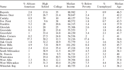
Below we use housing prices, which summarize information about neighborhood amenities, to select segments along the border where sorting seems to be less of a concern. We also provide a formal comparison of schools in Milwaukee county in Section A.2 in the Appendix. Basic comparisons of Milwaukee to the surrounding suburbs demonstrate that the city is more ethnically diverse, has lower housing prices, and lower socio-economic status. Census data from 2000 also reveals clear divisions between the city and its immediate suburbs. Median household income in Milwaukee is just under $34,000, whereas it is nearly $54,000 in the suburbs. The percentage of African-American residents that are of voting age in Milwaukee is 29 percent, whereas it is <1.5 percent in the suburbs. The difference in median housing value is nearly $60,000. Although the percentage of high-school graduates is nearly identical, nearly 21 percent in the suburbs have a college degree, whereas just over 12 percent in the city have a college degree. In Section A.3 in the Appendix, we provide more detailed comparisons and a map that shows spatial variation in racial residential patterns. Although the city of Milwaukee as a whole is clearly quite different from its suburbs, in terms of research design the crucial question is whether citizens near the city limit are more similar than what we observe based on full samples of residents.
Data
We use the Ohio and Wisconsin voter files, the databases of registered voters maintained by each state for administrative purposes to record voting outcomes. Both voter files also contain a limited number of covariates: date of birth, gender, and voting history. The Ohio voter file records party registration but not race, whereas the Wisconsin voter file records neither race nor party registration. To better understand how the treated and control areas might differ, we also use data from housing sales. Data from housing sales have a number of advantages. First, according to hedonic pricing theory, a house can be seen as a bundle composed of different attributes, and house prices can be used to infer the implicit prices of these attributes, which include not only physical characteristics of the house but also environmental characteristics of the neighborhood where the house is located, such as school quality, safety, etc. Models of hedonic house prices have been used, for example, to estimate the cost of local tax rates and to measure environmental quality (for reviews, see Sheppard Reference Sheppard1999; Malpezzi Reference Malpezzi2002). Second, these data are not aggregated, which allows us to precisely estimate how they vary around the boundary of interest. To that end, we acquired records for all houses sold in the appropriate zip codes in Cuyahoga County, Ohio, from 2008 to 2010, and in Milwaukee county, Wisconsin, from 2006 to 2008. There were nearly 5000 houses sold in and around Garfield Heights and nearly 30,000 houses sold in Milwaukee county during the time periods we study.
We also made limited use of census data. First, we collected block-level data. Blocks are the lowest unit of census geography, but the number of covariates available at this level is limited. At the block level, we have measures for the percentage of African-Americans and Hispanics, as well as median age. For the 2000 Census, block group-level data provide a richer set of covariates such as education and income. The drawback is that a block group contains between 600 and 3000 people. Given the large size of block groups, it is often difficult to tell whether there is meaningful spatial variation in block group-level measures as one approaches the boundaries of interest. For example, all of Garfield Heights is covered by fewer than eight block groups. Finally, we also collected electoral data, including partisan vote shares for federal offices and the governor as well as aggregate turnout measures for the two elections before the treated election. In Ohio, electoral data estimates are available at the census block level; in Wisconsin, electoral results are aggregated to wards, which are equivalent to precincts. In the next section, we describe how we used geographic information systems (GIS) software to process and geo-reference our data.
In both of the applications that follow, past turnout behavior would appear to be an important pretreatment covariate to either condition on or use as a placebo outcome. That is, in both cases past turnout is known to be unaffected by the ballot initiatives we study in 2008 and 2010. However, past turnout might be affected by other initiatives in previous elections. For example, in 2006, the residents of Milwaukee voted on an anti-Iraq War initiative that was not on the ballot in the suburbs, implying that past turnout is not strictly treatment free. This is less of a concern in Ohio given that 2008 was a presidential election. In this case, we expect that any local-level initiative would be of little consequence compared with the turnout efforts of presidential campaigns in a battleground state. For these reasons we avoid conditioning on past turnout in our analyses.
Geographic Analysis
We use GIS software to process the data before the final statistical analysis. We argue that without GIS analysis, geographic natural experiments are significantly weakened. GIS software allows analysts to more fully exploit geography and spatial proximity. We now outline the geographic analysis we performed to implement the different designs in Garfield Heights and Milwaukee county.Footnote 6
First, we geocoded both the voter file and data on housing sales. Geocoding is the process of converting addresses into a coordinate system, typically latitude and longitude. Geocoding allows us to know the distance between voters and the boundary of interest,Footnote 7 and, in the case of the GRD design, to develop a score that reflects the two dimensions of geographic space. Once we completed the geocoding, GIS software also allowed us to merge the individual-level data from the voter file with covariates collected from larger geographies such as census blocks and wards.Footnote 8
Second, we used the latitude and longitude obtained from the geocoding to calculate the spatial—or two-dimensional—distance between voter residences and the city limit directly. A simple application of the Euclidean distance with the points defined by latitude and longitude would be appropriate if voters resided in a plane, but the Earth is a sphere. As naive Euclidean distances calculated between geographic locations can severely overestimate the distance, we used the chordal distance, a rescaling of the Euclidean distance that incorporates the earth’s curvature (see Banerjee Reference Banerjee2005).
Finally, we used GIS software for a number of smaller tasks in our Milwaukee and Ohio examples. First, we created what is called a buffer around the city limit. The buffer is a spatial object that records which voters fall within a specified distance of a geographic boundary. We used a buffer to identify which voters are within 50, 100, 200, 300, 400, 500, 750, and 1000 meters from the city limit. Second, we used GIS to obtain a grid of points on the city limit for the calculation of treatment effects. We did this by dividing the Milwaukee city limit into points defined by latitude and longitude, spaced at intervals of at least 1 km. In Ohio, we used GIS to select final area of analysis—the area inside the Cleveland school district highlighted in Figure 2.
Results
As we noted in the second section, a number of different assumptions about geography may be invoked for the identification of causal effects. In the analyses that follow, we provide estimates under different identification strategies and evaluate whether exploiting geography directly appears to improve the credibility of the design. To that end, we focus on both the plausibility of the assumptions outlined in the second section and how inferences change as a function of conducting estimation based on each of these assumptions.
Garfield Heights
We first present the results from Garfield Heights, Ohio. We start with estimates based on assumptions that exploit geography in a very limited way: we estimate the average difference in turnout rates between the city of Garfield Heights and all adjacent cities, and then the average treatment effect controlling for a number of covariates via linear regression. As we do exclude some parts of Ohio and focus on one suburb of Cleveland, we have done some limited geographic conditioning. These estimation strategies are based on Assumptions 1 and 2, respectively. As shown in Table 1, in both cases the estimate indicates that turnout was nearly 4 percentage points higher in Garfield Heights. As mentioned in the second section, an analysis of this type does little to exploit geography, and we would not classify this as a natural experiment in that treatment assignment is entirely a function of decisions by voters and is not haphazard in any way. As such, there is little to suggest that the estimated effect is not contaminated by unmeasured confounders.
Garfield Heights, Ohio: Initiative Effect Estimates Under Differing Assumptions

Note: point estimates are recorded as percentages. Estimation under geographic ignorability assumption uses no covariates for adjustment. Estimation under geographic conditional ignorability adjusts age, age squared, Democratic vote share for president and US House in 2008, Democratic vote share for US Senate and House in 2006, percentage of Hispanic, percentage of African-American, percentage of Asian, percentage of owner-occupied housing, percentage of vacant housing, aggregated turnout from 2008 and 2006. SEs are adjusted for clustering at the block level.
An alternative research design exploits geography more carefully in hopes of finding a treatment assignment mechanism that is closer to as-if random. To that end, we could apply a Geographic Local Ignorability (GLI) or a GRD design. In both cases, we would use geographic information to compare voters just outside Garfield Heights with voters just inside Garfield Heights. Both designs would be more compelling if residents sorted around the Garfield Heights city limit in an as-if random fashion, an assumption we believe is plausible in the area of overlap between the city limit and the Cleveland school district in northeastern Garfield Heights. In this area, residents on both sides of the Garfield Heights city limit reside in the same school district and we are able to avoid other compound treatments in this location. For these reasons, we restrict our analysis to this small segment of the city limit, and the small area surrounding it. Given that the border between the two areas is short, the area of analysis is small, and we have strong evidence of covariate balance in this small area (see below), a GLI design based on Assumption 4 appears appropriate for this application.
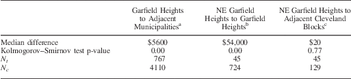
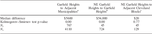
To better understand the plausibility of our identification assumption, we perform a balance analysis on three different housing price comparisons. First, we compare Garfield Heights to the entire surrounding metropolitan area. Second, we compare census blocks that are within both the Garfield Heights municipality and school district to census blocks that are within the Garfield Heights municipality but within the Cleveland school district. Finally, we compare census blocks within the Cleveland school district and Garfield Heights to the nearest set of census blocks that are also within the Cleveland school district but in the city of Cleveland. These comparisons will help us understand whether Garfield Heights appears to be generally different from the areas around it, and whether a clear discontinuity exists at the school district border.
The results of this analysis, reported in Table 2, are striking. First, houses in Garfield Heights are typically more expensive than those in adjacent municipalities, with a median difference of $5600. We tested for equality of the two distributions with the Kolmogorov–Smirnov (KS) test, and the p-value is statistically significant (p<0.001). When we compare prices for houses in the area of Garfield Heights that is inside the Cleveland school district to prices for houses in the rest of Garfield Heights, the median difference is substantial at $54,000. This comparison suggests that residents sort around the school district boundary between Cleveland and Garfield Heights. However, when we compare the same northeastern area of Garfield Heights to nearby census blocks in Cleveland, a comparison that keeps the school district constant, the median difference is a mere $20 with a KS test p-value of 0.77.Footnote 9 Based on this evidence, it appears that the part of Garfield Heights that shares schools with Cleveland is comparable with that part of Cleveland.
Garfield Heights, Ohio: Balance Test for Housing Prices
Note:
a Comparison of all houses sold within the zip codes that surround Garfield Heights with all houses sold within Garfield Heights from 2008 to 2010.
b Comparison of all houses sold within Garfield Heights that are not in Cleveland city school districts with all houses sold within Garfield Heights that are in Cleveland city school districts.
c Comparison of all houses sold within Garfield Heights that are in Cleveland city school districts with all houses sold in the nearest 42 census blocks in Cleveland and are in the same school district.
Given the results from the balance analysis, we think that a GLI design is plausible in the area where the Cleveland school district overlaps with northeastern Garfield Heights. Here, we can more forcefully argue that it might be an accident that someone lives in Garfield Heights rather than Cleveland. By basing our inference on the GLI design as characterized by Assumption 4, geography serves as useful method for reducing heterogeneity through a more focused comparison where treated and control units are clearly more comparable. As a result, we estimated the initiatives treatment effect by comparing turnout in the part of Garfield Heights within the Cleveland school district to turnout in the adjacent parts of Cleveland.
We estimate results with a simple difference in means for voters in this local area. As a comparison, we also estimate the effect under Assumption 4.b, using a linear regression specification to condition on age, party identification, the percentage of voters that are African-American or Hispanic, and the percentage of vacant houses. There is no need to condition on legislative districts as all of Garfield Heights falls within the same state and US legislative districts. With the exception of the first two measures, these covariates are census block-level measures. The results are in Table 3. The simple estimate of the treatment effect in this local area, at nearly 10 percentage points, is much larger than the estimates in Table 1. Conditioning on covariates decreases the magnitude of the effect, but this estimate is still double what we found when we conditioned on the same covariates in a larger geographic area. Given the empirical evidence based on housing prices, these estimates are far more credible than those based on global ignorability assumptions.
Garfield Heights, Ohio: Initiative Effect Within Areas with Overlapping School Districts

Note: point estimates are recorded as percentages. Treated area is the northeast part of Garfield Heights that is within the Cleveland school district. Control area consists of 42 nearest census blocks that are within the city limits of Cleveland.
Milwaukee
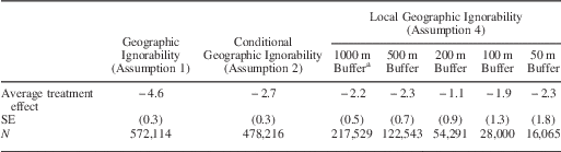
We now estimate the effect of initiatives on turnout in Milwaukee. As in the Garfield Heights example, instead of presenting one estimate from a single design, we proceed by exploring whether our estimates change depending on the identification assumption we invoke. We start with estimates based on Assumptions 1 and 2, which do not directly exploit geography. We first estimate the average difference in turnout rates between the city of Milwaukee and its suburbs, and then the same average treatment effect controlling for a number of covariates in a linear regression. The first two columns of Table 4 contain both estimates, and in both cases turnout is lower in Milwaukee.
2008 Milwaukee Ballot Initiative Effect Estimates Under Differing Assumptions
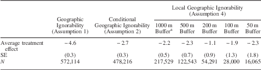
Note: estimation under geographic ignorability assumption uses no covariates for adjustment. Estimation under geographic conditional ignorability adjusts for sex, age, age squared, percentage of minority, percentage of African-American of voting age, median income, median housing value, percentage of housing units that are owner occupied, percentage with a high-school degree, percentage with a college degree, Democratic vote share for president and US House in 2004, Democratic vote share for governor and US Senate in 2006, and fixed effects for US House district and state legislative districts. SEs adjusted for clustering at the block level.
a A buffer is a band of specified distance width around the Milwaukee city limit. Estimates within geographic buffers are the average treated minus control difference for all voters who live within the specified distance from the city limit.
Next, we condition on distance alone using a GLI design under Assumption 4. We estimate effects by taking the average difference in turnout rates between the city and suburbs for those that live within a set distance from the city limit. Specifically, we define bands or buffers of 50, 100, 200, 500, and 1000 meters on either side of the Milwaukee city limit and calculate the average treatment effect for voters within each band via regression. We adjust standard errors for clustering within census blocks, and we do not use any covariates. The estimates are shown in the last five columns in Table 4, and are between −1 and −2.3 percentage points. That is, turnout in Milwaukee was typically lower in 2008 even in areas near the city limit. What is notable is that conditioning on distance buffers alone plays a very similar role to conditioning on covariates: the estimate in column 2 is generally similar to the buffer estimates.
Next, we turn to a GRD design based on Assumption 5. We avoid implementing this design in a naive way, as a simple examination of municipal-level census data suggests that there is high heterogeneity along the Milwaukee city boundary. For example, median income in Milwaukee is $32,000, whereas in the suburb of Wauwatosa it is $55,000. However, median income in the suburb of West Allis, which is adjacent to Wauwatosa to the south, is $39,000.Footnote 10
We analyze different points along the boundary to capture this heterogeneity using the local linear estimator that is commonly used in RD designs (see, e.g., Hahn, Todd and van der Klaauw Reference Hahn, Todd and van der Klaauw2001; Porter Reference Porter2003; Imbens and Lemieux Reference Imbens and Lemieux2008). Keele and Titiunik (Reference Keele and Titiunik2015) discuss in detail the use of local polynomial estimation in geographic contexts. With this estimator, we choose a fixed number of points along the boundary, and estimate the treated and control differences at each point weighting each observation within a given bandwidth by its distance to the point. We chose a fixed 1 km bandwidth for all points, but we also estimated mean squared error (MSE) optimal bandwidths. As these MSE optimal bandwidths were in all cases larger than 1 km, our fixed bandwidth effectively undersmooths and ensures that inferences based on conventional p-values and confidence intervals are valid (see Calonico, Cattaneo and Titiunik Reference Calonico, Cattaneo and Titiunik2014b). We estimate effects in 85 points along the boundary—details about how the points were selected are given in the Appendix. We implemented estimation with the rdrobust software.Footnote 11 As we perform many tests, we adjust p-values to control the false discovery rate (FDR).
We plot the local effects on 2008 turnout in Figure 4, showing whether the estimated turnout differential at each location is statistically significant. Interestingly, we observe some clusters of significant and insignificant effects which suggests that the ballot initiative treatment effect does vary along the Milwaukee city limit. The flexibility of the local polynomial estimator comes at some cost in terms of interpretability, as we now have a large number of estimates. Table 5 contains a summary of the estimates. As summary we take the mean of the local estimates across all boundary points, which provides a measure of the average effect along the boundary if all points have equal density of observations. This mean is −2.36 percentage points.
Estimated differences in turnout for 2008 election along Milwaukee city limit Note: all p-values corrected for false discovery rate.
2008 Milwaukee Ballot: Initiative Effect Estimate Based on Local Polynomial Estimator

Note: estimates are recorded as percentages. Each of the 85 individual effects is estimated with a local linear estimator. The 85 boundary points cover the entire Milwaukee city limit.
We now probe the plausibility of Assumptions 4 and 5 with various analyses. Unlike the Garfield Heights example, school district boundaries in Milwaukee county overlap perfectly with the Milwaukee city limit. This naturally raises questions about the validity of Assumption 3. In addition, this also raises questions about Assumption 5, as there is ample evidence that individuals often choose their place of residence based, for example, on the quality of the schools in their neighborhood. If this type of sorting is pervasive, this threatens identification in the GRD design based on Assumption 5.
We first study whether housing prices vary along the boundary. Figure 5 contains a map of the area and plots the location of the local polynomial estimates for the house price differential, showing which of those estimates are statistically significant based on FDR-adjusted p-values. The local estimator shows that generally the house price differential is significant when we compare Milwaukee with Wauwatosa and insignificant when we compare West Allis with Milwaukee, which is consistent with the aggregate census data. In general, we observe considerable variability along the city limit in the house price differential.
Estimated treated-control differences in housing prices along Milwaukee city limit Note: all p-values corrected for false discovery rate.
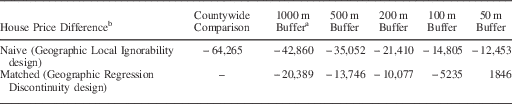
Next, we analyze whether differences in housing prices between the treated and control areas decrease as a function of distance to the city limit, which provides evidence regarding the plausibility of Assumption 4. We repeat the buffer analysis in Table 4, but this time using house sale prices as the outcome variable. These difference in means estimates within each buffer allow us to observe whether imbalances in housing prices decrease as a function of naive distance as measured by different buffers. We then match each treated unit within each buffer to the closest control unit, where the closest control is defined as the control unit whose chordal distance to the treated unit is lowest. Importantly, we do not apply matching as method of covariate adjustment; instead, we use matching on distance to assess whether balance in housing prices improves as a function of distance to the discontinuity. If the GRD design is more appropriate than the GLI design, the house price differential between treated and control areas should decrease within buffers as a function of non-naive distance to the city limit. For the matching analysis, we rely on nearest-neighbor matching with replacement and ties are broken randomly.
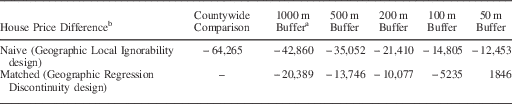
We report the average price differential between the city and the suburbs. As shown in the first column of Table 6, this difference is nearly $65,000. Restricting that comparison to housing sales within 1000 meters of the city limit drops the difference to nearly $43,000. This imbalance decreases with smaller buffers; however, even within 50 m the difference remains over $12,000. This analysis shows that conditioning on a buffer around the boundary as small as 50 meters is not enough to eliminate imbalances in housing prices. When we use the chordal distance to ensure close spatial (two-dimensional) proximity as opposed to naive proximity within buffers, the balance is much improved, as shown in the second row of Table 6. The differential within the 1000 m buffer is just over $20,000, compared with over $40,000 with the naive distance. For the 100 m buffer, the difference is just over $5000 and is less than $2000 for the 50 m buffer. This estimate is, however, statistically significant.
Covariate Balance on Housing Prices Between Milwaukee and Immediate Suburbs as a Function of Distance
Note:
a A buffer is a specified distance around the Milwaukee city limit. For example, with a 500 m buffer all voters who live more than 500 meters from the city limit are removed from the analysis before matching on geographic distance occurs.
b House price difference is the difference in dollars between the average house price in Milwaukee and its immediate suburbs. Rows labeled Naive show the unadjusted mean difference between treatment and control areas included in the buffer. Rows labeled Matched shows the mean difference between treatment and control areas included in the buffer after nearest-neighbor matching on chordal (spatial) distance alone.
The balance analysis suggests three things. First, the results clearly demonstrate that using geographic distance in a non-naive way in the context of a GRD design produces much better balance in a crucial pretreatment covariate. Second, it reveals that Assumption 5 is implausible in some points along the boundary. Third, we do observe improvement in balance as a function of geographic distance. This implies that conditioning on geography may strengthen this natural experiment, as an improvement in the balance of observed characteristics suggests that imbalances on unobservables may also improve as non-naive geographic distance is minimized.
We explore how the results from the local linear estimator change when we restrict the analysis to the points on the city limit where the house price differential is not statistically significant and the estimated difference in housing values is less than $5000.Footnote 12 This allows us to include the information of our “placebo map” (Figure 5) in our estimation stage, and restrict attention to those segments of the border where our identification assumption appears most plausible based on housing values. We also estimate a simple regression model that includes geographic proximity as an explanatory variable. In this specification, we use a cubic polynomial of the distance from the voter to the city limit. This model includes limited spatial flexibility in the estimation process, but does allow us to condition on a large number of pretreatment covariates.Footnote 13 As opposed to the first approach, the second approach will potentially mask heterogeneity. This method also imposes strong functional form constraints on geographic distance. To reduce heterogeneity further, we also restricted the analysis to voters who lived within 500 meters of the Milwaukee city limit. We also condition on the same set of covariates used to generate the estimates in column 2 of Table 4, including fixed effects of legislative districts.
We start with the results from the local estimator. In Figure 6, we plot the location of the conditional 2008 turnout estimates. We denote whether the estimated turnout differential at each location is either (i) statistically insignificant, (ii) statistically significant and in a location where the housing estimate was also significant, or (iii) statistically significant and in a location where the placebo test is passed (i.e., where the house price differential is not statistically significant and is less than $5000). Of the 85 points we analyzed along the city limit, 24 had a statistically significant turnout difference, and 12 of those estimates were at points that passed the housing value placebo test.
Estimated differences in turnout for 2008 election along Milwaukee city limit Note: all p-values corrected for false discovery rate.
The first column of Table 7 contains a summary of the turnout difference estimates for locations where the house price differential was insignificant and less than $5000, reporting a simple mean of the local point estimates. For these locations, the mean difference was just over one and half percentage points and the average p-value was 0.32. Thus, we find little evidence from this analysis that the ballot initiative increased turnout, as we have mostly insignificant results and a mean point estimate that is negative instead of positive as the hypothesis suggests. Table 7 also contains the regression estimates (second column); in this case, the ballot initiative effect is positive but is not statistically significant despite the fact that there are >100,000 observations.
2008 Milwaukee Ballot Initiative Effect Estimates Conditional on Geography and Covariates

Note: point estimates are recorded as percentages. In column 1, the effect reported is the mean of local linear estimates on housing prices for all points on the Milwaukee city limit where the difference in house prices was not statistically significant and was less than $5000 (and p-value reports the mean false discovery rate-adjusted p-value across the points). Regression estimate in column 2 is restricted to observations within 500 meters of the city limit and includes latitude and longitude as right-hand side covariates. The model also adjusts for sex, age, age squared, percentage of minority, percentage of African-American of voting age, median income, median housing value, percentage of housing units that are owner occupied, percentage with a high-school degree, percentage with a college degree, Democratic vote share for president and US House in 2004, Democratic vote share for governor and US Senate in 2006, and fixed effects for US House district and state legislative districts. SEs are adjusted for clustering at the block level.
Conclusion
Often natural experiments are the only means available to make a compelling case that an estimated correlation is causal. We have reviewed different assumptions that may be invoked in the presence of geographically varying treatments to produce valid casual effects. We have given particular attention to the GLI design and the GRD design, where in both cases the analyst compares units close to a border that separates adjacent treated and control areas. In the hierarchy of geographic natural experiments, designs that exploit the adjacency of treated and control areas are often the most promising. Treatments that vary with borders are ubiquitous in political science, as many political institutions often change sharply at geographic boundaries.
In both the GLI and GRD designs, pretreatment covariates should be similar near the boundary, which provides a clear and testable implication of the key identification assumption in each design. The difficulty facing both designs is that they are particularly vulnerable to a violation of their key identifying assumptions, because quite often agents are able to sort very precisely around the boundary that separates the areas of interest. If this sorting becomes too precise, the identification assumptions may not hold. Thus, understanding whether a specific GLI or GRD design allows for identification of the parameter of interest requires substantive knowledge and careful evaluation of how observable characteristics behave as distance to the boundary decreases. If balance in important pretreatment characteristics does not improve as function of distance, then the designs might not be credible.
Another obstacle that researchers may face when using geographic variation to make causal inferences is that it might be difficult to separate the effect of the treatment of interest from other features of the geographic unit. That is, the Compound Treatment Irrelevance assumption may not be very compelling in many contexts. In our applications, we sought to isolate the effect of ballot initiatives on turnout. In Garfield Heights, we were able to separate the boundary of interest from other borders. But in Milwaukee, it was impossible to isolate the city limit. When several borders coincide, the likelihood that units are precisely sorting on at least one of the borders increases, undermining the plausibility of geographic designs. When we were able to isolate the city limit from school district boundaries in Ohio, the difference in housing prices between both sides of the border shrank dramatically, giving strong credibility to the design. In Milwaukee, the GRD design exhibited some credibility given that the difference in housing prices became quite small near the city limit, but one can still imagine many unobserved confounders that may account for why one might live in the suburbs as opposed to the city of Milwaukee. This is not to say that the GRD design does not have advantages in this example. Given how balance improves as a function of distance, it suggests that a comparison along the Milwaukee city limit is worth exploiting as a discontinuity instead of relying on standard model-based methods with specification assumptions. But overall, we think our Wisconsin example illustrates many of the difficulties that geographic natural experiments may face, whereas our Ohio example illustrates the advantages that those designs can provide when their assumptions are reasonable.
Our empirical applications illustrate the general point that research designs usually become more credible when they are more local. That is, by focusing on small homogeneous geographic areas, we are more confident that people who look comparable are comparable. Whether this is achieved by invoking a GLI or a GRD design should depend on whether Assumption 4 or 5 is most plausible. In particular, when the border is long, the naive measure of distance employed in the GLI design will tend to be inappropriate and a GRD design may be preferable. Finally, the framework we have developed hinges crucially on the availability of high-quality geographic data. Unless the analyst can accurately define geographic locations, he or she may have little choice and be forced to estimate spatially constant effects.
In sum, while GLI and GRD designs may be vulnerable to violations of their identifying assumptions, geographic natural experiments can also make strong designs in that, given geo-referenced data, they can provide rich information about the behavior of pretreatment covariates (and even pretreatment or “placebo” outcomes) along the border; however, the plausibility of these designs can only be evaluated on a case-by-case basis. There is little hope that GLI and GRD designs can be mass produced, as they require careful attention to not only the statistical analyses needed to justify their assumptions, but also to the geographic analysis needed to fully assess their plausibility and exploit the variation that occurs at the geographic boundary.
Appendix
A.1 Ballot Initiative Text
The exact language on the ballot in Garfield Heights was as follows:
An amendment to the Charter of the City of Garfield Heights to enact Section 59 to limit use of photomonitoring devices to detect certain traffic law violations.
An amendment to the Charter of the City of Garfield Heights to enact Section 60 to abolish the tax on trash collection enacted by the Council and prevent any such future enactment.
The exact language on the ballot in Milwaukee was as follows:
Shall the City of Milwaukee adopt Common Council File 080420, being a substitute ordinance requiring employers within the city to provide paid sick leave to employees?
A.2 Milwaukee School Performance Analysis
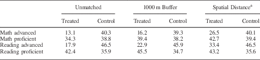
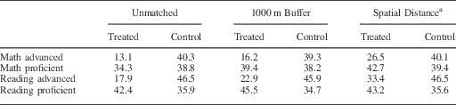
In the main analysis, we examined whether a large number of covariates changed discontinuously at the Milwaukee city limit. One covariate that we did not include in the analysis is a measure of school quality. We excluded measures of school quality because house prices should reflect differences in local school quality. Several papers in the economics literature have established that houses in areas with better schools demand a price premium (Black Reference Black1999; Lavy Reference Lavy2006; Bayer, Ferreira and McMillan Reference Bayer, Ferreira and McMillan2007). As such, any difference in school quality between Milwaukee and its suburbs should be reflected in our analysis of housing price differentials. Despite this, we did examine data on school quality. To assess the difference between schools in and outside of Milwaukee, we used results from the Wisconsin Knowledge and Concepts Examination (WKCE) from the Wisconsin Student Assessment System. The WKCE is a large-scale, standardized achievement test given to all students in grades 4 and 8 and includes sections on reading, language, arts, mathematics, science, and social studies. The state of Wisconsin does not release test scores for specific schools, but instead reports the percentage of students that are advanced, proficient, basic, or minimally performing.
In Milwaukee county, there are 172 elementary schools that administered the WKCE to 4th grade students. We collected the addresses for all of these schools and geocoded them to obtain latitude and longitude and calculate distances to the city limit. The state of Wisconsin rates schools by the percentage of students that are advanced or proficient. Table A1 contains the results from three comparisons. We only compared school performance on the reading and math components of the exam, and we averaged results from 2006 and 2007 to remove chance fluctuations. The first comparison is based on all schools in the city of Milwaukee and all schools in the suburbs. The key difference between Milwaukee and its suburbs is that a much larger percentage of students are classified as advanced in the suburbs. To make the comparison more local, we next restrict the analysis to the Milwaukee schools that are no more than 1000 meters away from the city limit. We see modest improvement as the percentage of students that are classified as advanced increases slightly. We next match on spatial distance within the 1000 m buffer. Now the gains are more substantial. Although suburban schools still have a higher percentage of advanced students, the gap between the city and suburbs is reduced from a gap of 27.2 and 28.6 percentage points to 13.6 and 13.1 percentage points for mathematics and reading, respectively. This fits with our general pattern of improvement in covariate balance as we get closer to the city limit.
A.3 Baseline Comparisons Between Treated and Control Areas
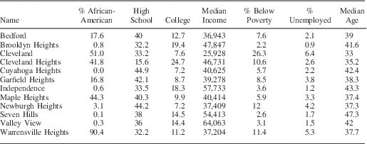
Here we provide additional information on how Milwaukee and Garfield Heights differ from the surrounding municipalities. First, in Figure A1 we map spatial variation in racial residential patterns in Milwaukee. This map clearly demonstrates that African-Americans primarily live in the northern part of the city, and in this region there are stark differences between Milwaukee and the suburbs. In the southern part of the city, however, we see that differences are less stark. Suburbs such as West Allis, Greenfield, and St. Francis have racial patterns that are very comparable with adjacent areas in Milwaukee. These differences closely match what we find applying the local polynomial estimator to housing prices. Table A2 contains a comparison between Milwaukee and its immediate suburbs using census data from 2000. As we noted in the text, Milwaukee differs substantially from many of the suburbs. Table A3 contains a comparison between Garfield Heights and its immediate neighbors using census data from 2000.
Racial composition in Milwaukee at the census block level Source: 2000 Census. Note: colors represent the percentage of African-Americans who are of voting age by census block.
Balance on School Test Scores Between the City of Milwaukee and its Suburbs
Census Profiles of Milwaukee and its Immediate Suburbs
Census Profiles of Garfield Heights and Surrounding Municipalities
A.4 Selection of Boundary Points and Bandwidth
We initially chose bandwidths using data-driven selection procedures that minimize a MSE criterion specially suited for estimating a discontinuity jump in the regression function (see Imbens and Kalyanaraman Reference Imbens and Kalyanaraman2012; Calonico, Cattaneo and Titiunik Reference Calonico, Cattaneo and Titiunik2014b). In some cases, however, these optimal procedures could not deal adequately with sparse boundary points where there are no observations close to the border. This mostly occurred in non-residential areas along the Milwaukee border. For example, the Milwaukee city limit falls exactly on the outer limit of the Milwaukee airport. To address this issue, we developed a criterion to decide whether a boundary point was sparse (in which case it was excluded from the analysis).
We first divided the Milwaukee city into ~143 boundary points separated by 1 km. For every point, we set a fixed bandwidth of 1 km, and calculated the number of observations that received positive weights with a triangular kernel. We did this for the treated and control observations separately. When this minimum number of observations was below 100 in either the treated or the control group, the point was declared sparse and no estimation was performed at that point. For all remaining points that satisfied the minimum observations requirement, we calculated the minimum and the 10th percentile of the distances of each unit to the boundary point, for observations in the treated and the control areas separately. When the minimum distance was ≤0.10 km and the 10th-percentile distance was ≤0.50 km, the points were included in the analysis. The remaining points were declared sparse and no estimation was performed for them. Close inspection of Figures 4 and 5 reveals that the algorithm clearly excludes areas that are non-residential for a number of reasons. We included 85 boundary points in our final analysis. We then used the fixed 1 km bandwidth for analysis in these 85 non-sparse points. As mentioned in the text, for all the points included in the analysis, the MSE optimal bandwidths were larger than 1 km, which means that our fixed 1 km bandwidths effectively undersmooth and the leading asymptotic bias in the conventional distributional approximation becomes negligible. This means that inferences based on conventional confidence intervals and p-values are valid. See Calonico, Cattaneo and Titiunik (Reference Calonico, Cattaneo and Titiunik2014b) for details, and for a robust alternative to conventional confidence intervals that leads to valid inferences even in the absence of undersmoothing.