1 Introduction
Problems of partial differential equations are often defined on an unbounded domain. Solving those problems numerically in a straightforward way would also require unbounded (i.e. infinite) memory and calculation time, which we do not have. Thus, we have to restrict the computational domain to a finite subdomain of the full problem. At the boundary of the computational domain, we set up artificial boundary conditions (BCs), which are meant to approximate the interaction with the outside area. Modelling such an open boundary is especially difficult in time-dependent, dynamic problems.
In plasma simulations, homogeneous Neumann BCs, sometimes known as zero normal derivative conditions, have been widely used for open boundaries (Shibata & Uchida Reference Shibata and Uchida1985; Scholer Reference Scholer1989; Stone & Norman Reference Stone and Norman1992; Yan, Lee & Priest Reference Yan, Lee and Priest1992; Fromang & Nelson Reference Fromang and Nelson2006; Huang & Bhattacharjee Reference Huang and Bhattacharjee2010; Tretler, Tatsuno & Hosokawa Reference Tretler, Tatsuno and Hosokawa2020). This will enable the physical quantities at the boundaries to change in time; however, it does not necessarily mean that the outgoing waves leave the domain since the standard wave equation with this condition brings about free end reflections. Thus we often need a sufficiently large domain so that the reflected waves do not affect the dynamics of interest.
To reduce these unphysical reflections, multiple specialized BCs have been constructed (Tsynkov Reference Tsynkov1998; Tourrette & Halpern Reference Tourrette and Halpern2001; Colonius Reference Colonius2004) including the ones in some plasma applications (Sato & Hayashi Reference Sato and Hayashi1979; Dedner et al. Reference Dedner, Kröner, Sofronov and Wesenberg2001; Meier, Glasser & Shumlak Reference Meier, Glasser and Shumlak2012). We can classify the BCs by whether they are defined on a surface or on a layer. The Mur absorbing boundary condition (ABC) (Mur Reference Mur1981) for linear wave equations, which assumes outward propagations with appropriate wave speeds on boundaries, is an example of a surface BC. On the other hand, the perfectly matched layer (PML) (Berenger Reference Berenger1994; Kako & Ohi Reference Kako and Ohi2005), which absorbs waves in a fictitious absorbing layer at the exteriors of the computational domain, is an example of a layer BC. Generally, layer BCs require a larger computational domain (for the layer) than surface BCs, which means their costs tend to be higher as well; however, they also tend to have a stronger absorbing effect. Fictitious absorbing layers based on the PML are implemented in several fluid (Hu Reference Hu1996; Nataf Reference Nataf2006; Hu, Li & Lin Reference Hu, Li and Lin2008; Lin, Li & Hu Reference Lin, Li and Hu2009; Sonoda, Ohi & Tatsuno Reference Sonoda, Ohi and Tatsuno2017) and plasma (Hanasoge, Komatitsch & Gizon Reference Hanasoge, Komatitsch and Gizon2010) models.
Waves passing through this layer would be absorbed at a rate depending on the distance from the boundary, which means that faster waves, that spent less time in the layer, could not be absorbed as well as slower waves. In other words, the effectiveness of this absorbing layer was inversely proportional to the waves’ phase velocity. The waves’ phase velocity is common to all scales in these fluid models (Hu Reference Hu1996; Nataf Reference Nataf2006; Hu et al. Reference Hu, Li and Lin2008; Lin et al. Reference Lin, Li and Hu2009; Sonoda et al. Reference Sonoda, Ohi and Tatsuno2017); however, they do change in various plasma models (Hasegawa & Uberoi Reference Hasegawa and Uberoi1982; Kingsep, Chukbar & Yan'kov Reference Kingsep, Chukbar and Yan'kov1990; Birn et al. Reference Birn, Drake, Shay, Rogers, Denton, Hesse, Kuznetsova, Ma, Bhattacharjee and Otto2001; Schekochihin et al. Reference Schekochihin, Cowley, Dorland, Hammett, Howes, Quataert and Tatsuno2009). Namely, the waves are ‘dispersive’ in many applications. In this research, we developed a new fictitious absorbing layer, which absorbs waves regardless of their phase velocity.
In this paper, we focus on the one-dimensional linear and nonlinear Schrödinger equations for a simple model of the dispersive wave. The many studies concerning ABCs for Schrödinger equation are described in a review article by Antoine et al. (Reference Antoine, Arnold, Besse and Schädle2008). For the finite domain approximation to the infinite domain linear Schrödinger equation, several BCs were independently derived from various application fields (Baskakov & Popov Reference Baskakov and Popov1991; Dalrymple & Martin Reference Dalrymple and Martin1992; Hellums & Frensley Reference Hellums and Frensley1994). There are also BC derivations for periodic or piecewise constant potentials (Ehrhardt & Zheng Reference Ehrhardt and Zheng2008; Zheng Reference Zheng2008). These methods are effective for the Schrödinger equation; however, they are non-local in time, which imposes a high memory cost, especially for multiple dimensions. Some alternative formulations, e.g. the pole condition (Ruprecht et al. Reference Ruprecht, Schädle, Schmidt and Zschiedrich2008; Ruprecht, Achädle & Schmidt Reference Ruprecht, Achädle and Schmidt2013) and PML (Zheng Reference Zheng2007) are local in time, which drastically lowers the computational cost. Most of the above BC derivations (Baskakov & Popov Reference Baskakov and Popov1991; Dalrymple & Martin Reference Dalrymple and Martin1992; Hellums & Frensley Reference Hellums and Frensley1994; Ehrhardt & Zheng Reference Ehrhardt and Zheng2008; Zheng Reference Zheng2008; Ruprecht et al. Reference Ruprecht, Schädle, Schmidt and Zschiedrich2008, Reference Ruprecht, Achädle and Schmidt2013) are made specifically for the linear Schrödinger equation and are difficult or impossible to use on other problems, such as nonlinear equations with no exact solution. However, since PML can, in general, be extended to nonlinear problems, we expect that the PML formulation of Schrödinger equation BCs can also be extended to nonlinear equations.
Zheng (Reference Zheng2007) successfully applied PML to the Schrödinger equation, in its one-dimensional and multidimensional, as well as linear and nonlinear, formulations. Therefore, we expect that PML can also be applied to other problems with dispersive waves. To improve understanding of PML for the Schrödinger equation, we propose and analyse several simple boundary layers motivated by Zheng's PML. With our simplified design based on dispersion relations, we focus on specific physical effects and investigate the effectiveness of various boundary layers on dispersive waves.
This paper is organized as follows. In § 2, we review the basic properties of the Schrödinger equation and describe the numerical method used and its stability. In § 3, we summarize Zheng's coordinate-stretching PML, after which we propose an alternative approach using damping and deceleration effects. In § 4, we elaborate on the alternative layers which damp or decelerate waves, and evaluate their performance. We then suggest a new type of absorbing layer made by combining the aforementioned effects. We also apply the proposed layer to a nonlinear Schrödinger equation in § 5, and finally give a brief conclusion in § 6.
2 Linear Schrödinger equation and its discretization
We use the following normalized linear Schrödinger equation without a potential:
 \begin{equation} \textrm{i} \partial_t u + \partial_x^2 u = 0, \end{equation}
where  $\textrm {i}$ is the imaginary unit and
 $u$ is the wavefunction
 $u(x, t)$. Let us consider the dispersion relation of this equation. Replacing
 $u$ in (2.1) with a Fourier mode,
 \begin{equation} u(x, t) = \varphi(k; x,t) := \exp(\textrm{i} k x - \textrm{i} \omega t), \end{equation}
we obtain
 \begin{equation} \omega = k^2, \end{equation}
where  $k$ is the wavenumber and
 $\omega$ is the angular frequency. This relation implies that a wave with a wavenumber
 $k$ travels with the phase velocity
 $v_\textrm {ph} = \omega /k = k$.
Ideally we would like to solve (2.1) over the infinite domain,  $\varOmega = ( - \infty , \infty )$. However, as we are constrained by limited computational resources, we need to reduce the computational domain to a finite size. We set the finite simulation domain to
 $\varOmega _{{D}} = [ x_{\textrm {LP}}, x_{\textrm {RP}} ]$ where
 $x_{\textrm {LP}}$ and
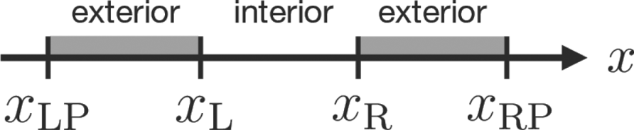
 $x_{\textrm {RP}}$ are the left-hand and right-hand boundaries of the computational domain (see figure 1), and use the centred finite difference method for spatial discretization with Crank–Nicolson (CN) method for time integration (Press et al. Reference Press, Teukolsky, Vetterling and Flannery2007).
Relation between the simulation domains and equations, with Schrödinger equation (2.1) in the interior domain and one or more layer equations in the exterior domains.

We note here that the solution  $u$ to the Schrödinger equation (2.1) satisfies the condition
 \begin{equation} \partial_t \int_{\varOmega} |u|^2 \,\textrm{d} x = 0, \end{equation}
where  $|u|^2$ is the particle existence probability, which is used later for confirming the stability of our discretization. In the computational domain
 $\varOmega _{{D}}$, the same condition
 \begin{equation} \partial_t \int_{\varOmega_{{D}}} |u|^2 \,\textrm{d} x = 0, \end{equation}
is required as long as the wave stays in  $\varOmega _{{D}}$.
Let  $N_x$ be a positive integer. Then, we take the spatial and temporal discretization step sizes as
 ${\rm \Delta} x = (x_{\textrm {RP}} - x_{\textrm {LP}}) / N_{x}$ and
 ${\rm \Delta} t$, respectively, and denote the grids by
 \begin{equation} x_j = x_{\textrm{LP}} + j {\rm \Delta} x, \quad t^{(n)} = n {\rm \Delta} t, \quad u (x_j, t^{(n)}) = u_j^{(n)}, \end{equation}
where subscripts  $j$ denote the spatial grid point
 $(\,j = 0, \ldots , N_x)$ and superscripts
 $(n)$ denote the time step
 $(n = 0, 1, \ldots )$. After discretization, (2.1) is
 \begin{equation} \textrm{i} \frac{ u_j^{(n+1)} - u_j^{(n)} }{ {\rm \Delta} t } = - \frac{1}{2} \left\{ \frac{ u_{j+1}^{(n)} - 2 u_j^{(n)} + u_{j-1}^{(n)} }{ {\rm \Delta} x^2 } + \frac{ u_{j+1}^{(n+1)} - 2 u_j^{(n+1)} + u_{j-1}^{(n+1)} }{ {\rm \Delta} x^2 } \right\}, \end{equation}
where  $j = 1, \ldots , N_x - 1$. At the boundary points
 $x_{\textrm {LP}}$ and
 $x_{\textrm {RP}}$, we apply homogeneous Dirichlet BCs,
 \begin{equation} u_0^{(n)} = u_{N_x}^{(n)} = 0. \end{equation}
Here, the discretization (2.7), (2.8) unconditionally satisfies the condition (2.5) as long as the support of  $u$ is in
 $\varOmega _{{D}}$ (Press et al. Reference Press, Teukolsky, Vetterling and Flannery2007). Note that this BC does not satisfy the original, ideal assumption of infinite domain. This issue will be addressed in § 3.
In the unbounded domain, the exact solution to the Schrödinger equation (2.1) with the Gaussian initial condition
 \begin{equation} u_\textrm{init} = \exp [ -(x - x_{\textrm{c}})^2 + \textrm{i} k_{0} (x - x_{\textrm{c}}) ], \end{equation}
where  $k_{0}$ is the characteristic wavenumber, and
 $x_{\textrm {c}}$ is the centre of the Gaussian, is (Antoine & Besse Reference Antoine and Besse2003; Antoine et al. Reference Antoine, Arnold, Besse and Schädle2008)
 \begin{equation} u_{\textrm{ex}} = \sqrt{ \frac{\textrm{i}}{-4t + \textrm{i}} } \exp \left( \frac{- \textrm{i} (x - x_{\textrm{c}})^2 - k_{0} (x - x_{\textrm{c}}) + k_{0}^2 t}{-4t + \textrm{i}} \right). \end{equation}
Here, for the square root of a complex number, we take the branch with the positive real part. This equation represents a travelling Gaussian beam with the velocity of its peak denoted by  $2k_{0}$. In the following simulations, we take a well-confined initial condition so that
 $u$ is sufficiently close to zero at the computational boundaries. As the simulation proceeds, the wave travels and hits the boundary, which we try to remove from the computational domain as cleanly as possible.
3 Fictitious absorbing layer
The PML was suggested by Berenger (Reference Berenger1994) and applied to Maxwell's equations. It was subsequently also applied to various other problems; linearized Euler equations (Hu Reference Hu1996; Nataf Reference Nataf2006), nonlinear fluid equations (Hu et al. Reference Hu, Li and Lin2008; Lin et al. Reference Lin, Li and Hu2009; Sonoda et al. Reference Sonoda, Ohi and Tatsuno2017) and linearized magnetohydrodynamics (MHD) equations (Hanasoge et al. Reference Hanasoge, Komatitsch and Gizon2010). In particular, Zheng (Reference Zheng2006, Reference Zheng2007) applied it to linear and nonlinear Schrödinger equations. We review Zheng's treatment briefly and show explicitly that it has the multiple effects of damping and deceleration.
3.1 Coordinate stretching
Zheng (Reference Zheng2007) applied a complex coordinate stretching
 \begin{gather} \bar{x} := x + R \varSigma (x), \end{gather}
 \begin{gather}\varSigma (x) := \int_{x_{{R}}}^x \sigma(r) \,\textrm{d} r, \end{gather}
to Schrödinger equations, which was first introduced by Chew & Weedon (Reference Chew and Weedon1994) for Maxwell's equations. Here  $R$ denotes a complex factor which introduces the damping effect, and is taken to be
 $R := \textrm {e}^{{\rm \pi} \textrm {i} /4}$ for a good performance (see figure 1 of Zheng Reference Zheng2007). The function
 $\sigma (x)$ is a continuous real function which vanishes in the interior and takes positive values in the exterior (PML) regions, respectively (see figure 1), where
 $x_{{R}}$ is the boundary between interior and exterior regions. It is noted that we focus on the right-hand exterior region in figure 1 and ignore the left-hand one in this section. In the exterior region, the unit length of
 $\bar {x}$ is smaller than the original
 $x$ since
 $\sigma (x)$ is positive; i.e. the original coordinate
 $x$ is stretched compared to
 $\bar {x}$. The specific form of
 $\sigma (x)$ used in our simulation will be presented later in (4.4). Then from
 \begin{equation} \frac{\partial}{\partial \bar{x}} = \frac{1}{1 + R \sigma(x)} \frac{\partial}{\partial x}, \end{equation}
the Schrödinger equation in  $\bar {x}$,
 \begin{equation} \textrm{i} \partial_t u + \partial_{\bar{x}}^2 u = 0, \end{equation}
is written in terms of the original coordinate  $x$ as
 \begin{equation} \textrm{i} \partial_t u + \frac{1}{1 + R \sigma(x)} {\partial_x} \left( \frac{1}{1 + R \sigma(x)} \partial_x u \right) = 0. \end{equation}
Since (3.4) is written in the same form with (2.1) in terms of the new coordinate  $\bar {x}$, it has an exact solution of the Fourier mode in
 $\bar {x}$,
 \begin{equation} u(x, t) = \varphi (k; \bar{x}, t) = \exp(\textrm{i} k \bar{x} - \textrm{i} \omega t). \end{equation}
Therefore, (3.5) also has the corresponding exact solution, written in terms of  $x$ as
 \begin{equation} u(x, t) = \exp(\textrm{i} k \bar{x} - \textrm{i} \omega t) = \exp \{\textrm{i} k [x + R \varSigma (x)] - \textrm{i} \omega t \}. \end{equation}
By splitting  $R$ into real (
 $R_{{r}}$) and imaginary (
 $R_{{i}}$) parts,
 \begin{equation} R = R_{r} + \textrm{i} R_{i}, \end{equation}
(3.7) may be written as
 \begin{equation} u(x, t) = \exp \{\textrm{i} k [x + R_{r} \varSigma (x)] - \textrm{i} \omega t\} \exp [- k R_{i} \varSigma (x)], \end{equation}
where we took  $x_{{R}} = 0$ for simplicity. Now, plugging (2.3) into (3.9), we obtain
 \begin{equation} u(x, t) = \exp \{ \textrm{i} k [x + R_{r} \varSigma (x) ] - \textrm{i} k^2 t \} \exp [- k R_{i} \varSigma (x) ]. \end{equation}
These solutions tell us that, at a fixed  $x$, they will oscillate with the frequency
 $k^2$, but the oscillation amplitude will not change in time for a given
 $k \in \mathbb {R}$. On the other hand, at a fixed
 $t$, the oscillation amplitude damps in
 $x$ according to
 $\exp [ - k R_{i} \varSigma (x) ]$ in the original coordinate
 $x$. The wavenumber changes into a complex number,
 \begin{equation} \underline{k} = k \left[ 1 + R \frac{ \varSigma (x) }{x} \right]. \end{equation}
Since  $R_{r} > 0$, the real part of the wavenumber
 $k$ in the original coordinate
 $x$ has increased, namely, the wavelength has shrunk by the factor
 $(1 + R_{r} \varSigma (x) / x )$. In the coordinate stretching (3.1), the unit length of
 $\bar {x}$ is smaller than the original
 $x$
 $(\mathrm {Re} \, \bar {x} > x)$; thus, a fixed wavenumber
 $k$ in
 $\bar {x}$ corresponds to a shrunk wavelength
 $(\mathrm {Re} \, \underline {k} > k)$ in the original coordinate
 $x$. It is noted that the argument by Zheng is exactly applicable to a spatially varying
 $\sigma (x)$.
3.2 Damping and deceleration
Here we consider the case with constant  $\sigma$ and take a Fourier analysis of (3.5) with respect to
 $x$. The spatially varying
 $\sigma (x)$ may be treated under the WKB approximation (Bender & Orszag Reference Bender and Orszag1999) when the spatial variation scale is large compared with the inverse of the wavenumber, say
 $k D \gg 1$, where
 $D$ denotes the PML layer width.
When  $\sigma$ is a constant,
 $\varSigma (x) = \sigma x$ will change (3.9)–(3.11) into
 \begin{gather} u(x, t) = \exp [\textrm{i} k (1 + R_{r} \sigma) x - \textrm{i} \omega t] \exp (- k R_{i} \sigma x ), \end{gather}
 \begin{gather}u(x, t) = \exp [\textrm{i} k (1 + R_{r} \sigma) x - \textrm{i} k^2 t ] \exp (- k R_{i} \sigma x) \end{gather}
and
 \begin{equation} \underline{k} = k(1 + R \sigma), \end{equation}
respectively. It is noted that the pseudo-Fourier mode  $\varphi (\underline {k}; x,t)$ with the complex wavenumber
 $\underline {k}$ is an exact solution to (3.5).
In the Fourier analysis with respect to  $x$, we should denote wavenumbers by
 $\underline {k}$ instead of
 $k$ since we handle the mode with a wavenumber for
 $x$; however, we would like to have a real wavenumber rather than the complex
 $\underline {k}$. In order to avoid confusion, we denote a wavenumber by
 $\tilde {k} \in \mathbb {R}$, regard it a constant in
 $x$, and decouple it from (3.14). Plugging
 \begin{equation} u(x, t) = \varphi (\tilde{k}; x, t) = \exp(\textrm{i} \tilde{k} x - \textrm{i} \omega t) \end{equation}
into (3.5) with the assumption of constant  $\sigma$ yields the dispersion relation
 \begin{equation} \omega = \left( \frac{ \tilde{k} }{1 + R \sigma} \right)^2. \end{equation}
Then (3.15) yields
 \begin{equation} u(x, t) = \exp ( \textrm{i} \tilde{k} x - \textrm{i} \omega_{r} t) \exp (\omega_{i} t), \end{equation}
where  $\omega _{r}$ and
 $\omega _{i}$ are real and imaginary parts of
 $\omega$ obtained from (3.16), respectively. This solution tells us that, at a fixed
 $x$, it will oscillate with the frequency
 $\omega _{r}$ and the growth (or damping) rate
 $\omega _{i}$ for a given
 $\tilde {k} \in \mathbb {R}$. It is noted that
 $\omega _{i}$ is always negative for
 $R=\textrm {e}^{{\rm \pi} i/4}$ and
 $\sigma > 0$. On the other hand, at a fixed
 $t$, the oscillation amplitude is constant along
 $x$. This may be directly obtained by rewriting (3.14) in terms of
 $k$ and replacing
 $k$ by
 $\tilde {k}$. The difference between (3.13) and (3.17) is whether we regard
 $k$ or
 $\tilde {k}$ to be real numbers, respectively. They are both exact solutions of (3.5) for a constant
 $\sigma$; one describes spatially damping oscillations making temporary stationary wave propagation, and the other describes spatially homogeneous solutions damping with respect to time.
According to (3.17), for  $t > 0$, the solution will decay exponentially at a rate of
 $|\omega _{i}|$. In addition, its phase velocity is reduced, since
 $\omega _{r} < \tilde {k}^2$. With this consideration, we find that (3.17) will have these two effects; damping and deceleration in isolation. We examine their impact on the wavefunction, and explore using them to construct an effective absorbing layer for a dispersive medium. In the following, we first use the idea of damping layers, which simply make the waves decay. Next, we investigate deceleration layers, which slow the waves down. Finally, we suggest a compound absorbing layer obtained by combining the two layer types.
4 Numerical tests
4.1 Damping layers
We add a damping term in the dispersion relation (2.3)
 \begin{equation} \omega = k^2 - \textrm{i} \sigma, \end{equation}
where the real constant  $\sigma$ is the damping factor. Dispersion relation (4.1) corresponds to a modified Schrödinger equation
 \begin{equation} \textrm{i} \partial_t u + \partial_x^2 u + \textrm{i} \sigma u = 0, \end{equation}
which we will call the damping layer equation. The damping strength of the wavefunction  $u$ depends on
 $\sigma$.
Let us examine the behaviour of the damping layer equation. We assume that the solution to (4.2) has the form (2.2). Substituting (4.1) into the solution (2.2), we obtain
 \begin{equation} u (x, t) = \hat{u} (x, t) \, \textrm{e}^{-\sigma t}, \end{equation}
where  $\hat {u}$ is the solution to the standard Schrödinger equation (2.1) with
 $k$ and
 $\omega$ replaced by
 $\hat {k} = k$ and
 $\hat {\omega }=\hat {k}^2$, respectively. We can see that the wavefunction in (4.3) is damped in time with a damping rate
 $\sigma$.
Solving the damping layer equation for the entire simulation domain does not give us the solution for the original Schrödinger equation (2.1). Instead, we first divide the simulation domain into the interior and the exterior domains. Next, we solve the Schrödinger equation (2.1) in the former, and the damping layer equation (4.2) in the latter. At the connecting points of interior and exterior domains, there is a difference between  $u$ and
 $\hat {u}$, which will cause numerical reflections in simulations. Therefore, we replace the damping factor
 $\sigma$ with an appropriate damping function
 $\sigma (x)$, which should allow a well-behaved approximation to (2.1) in the infinite domain. Rigorously speaking, the damping factor
 $\sigma$ in the dispersion relation (4.1) is supposed to be a constant. However, it is useful to admit a slow spatial dependence in
 $\sigma$ and regard (4.1) to hold in the WKB sense (Bender & Orszag Reference Bender and Orszag1999) hereafter.
We choose the interior end points  $x_{{L}}$ and
 $x_{{R}}$ such that
 $x_{\textrm {LP}} < x_{{L}} < x_{{R}} < x_{\textrm {RP}}$, and divide the simulation domain into the interior domain
 $[x_{{L}}, x_{{R}}]$ and two exterior domains
 $[x_{\textrm {LP}}, x_{{L}})$ and
 $(x_{{R}}, x_{\textrm {RP}}]$, as shown in figure 1. In the interior domain, we solve the Schrödinger equation (2.1). In the exterior domains, which we will call fictitious damping layers, we solve the damping layer equation (4.2). In order to smoothly combine the equations in these domains, we let the damping factor
 $\sigma$ be
 \begin{align} \sigma(x) = \begin{cases} \sigma_0 \left( \dfrac{x - x_{{L}}}{D_{{L}}} \right)^2 & (x_{\textrm{LP}} \leq x < x_{{L}}), \\ 0 & (x_{{L}} \leq x \leq x_{{R}}), \\ \sigma_0 \left( \dfrac{x - x_{{R}}}{D_{{R}}} \right)^2 & (x_{{R}} < x \leq x_{\textrm{RP}}), \end{cases} \end{align}
where the constant  $\sigma _0$ is the maximum value of
 $\sigma (x)$ in the external domains, and
 $D_{{L}}$ and
 $D_{{R}}$ are widths of, respectively, the left-hand and right-hand damping layers. We use the quadratic function for
 $\sigma (x)$ in (4.4) to reduce the numerical error due to reflected waves (Berenger Reference Berenger1994; Zheng Reference Zheng2007; Sonoda et al. Reference Sonoda, Ohi and Tatsuno2017).
In the following sections, we compute the layer equations with parameters taken from Antoine et al. (Reference Antoine, Arnold, Besse and Schädle2008). We use a centred finite difference CN scheme (2.7) with  ${\rm \Delta} x = 0.01$,
 ${\rm \Delta} t = 10^{-3}$ unless noted otherwise. For the initial value we use the Gaussian (2.9) with
 $k_{0} = 5$,
 $x_{\textrm {c}} = 6$, and set the interior domain to
 $[x_{{L}}, x_{{R}}] = [0, 15]$. To evaluate the accuracy of the approximation, let the relative numerical error
 $u_{\textrm {err}}$ be
 \begin{equation} u_{\textrm{err}} = \frac{||u_{\textrm{sim}} - u_{\textrm{ex}}||_{[x_{{L}}, x_{{R}}]}} {||u_{\textrm{init}}||_{[x_{{L}}, x_{{R}}]}}, \end{equation}
where  $u_{\textrm {sim}}$ is the numerical value of the wavefunction,
 $u_{\textrm {init}}$ and
 $u_{\textrm {ex}}$ are given by (2.9) and (2.10), and
 $||u||_{[x_{{L}}, x_{{R}}]}$ is the
 $L^2$ norm over the domain
 $[x_{{L}}, x_{{R}}]$.
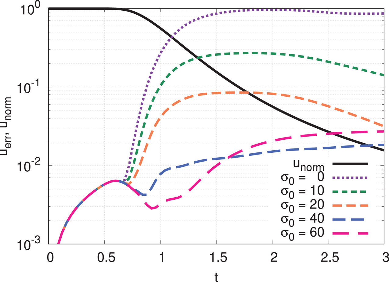
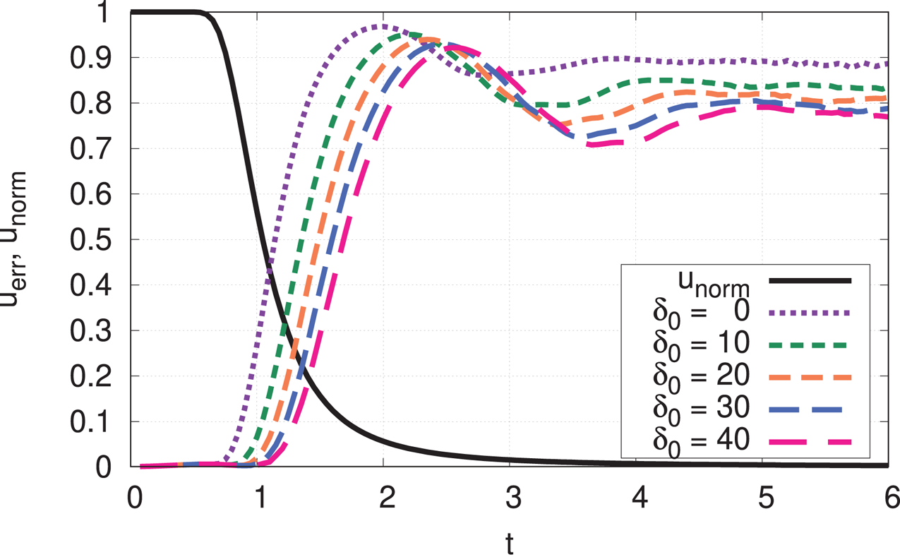
Figure 2 depicts the numerical error for several damping factor maximum  $\sigma _0$. The thickness of the damping layers at left- and right-hand exterior regions are
 $D_{{L}} = D_{{R}} = 2$, i.e.
 $[x_{\textrm {LP}}, x_{\textrm {RP}}] = [-2, 17]$. The black curve is the normalized
 $L^2$ norm of the exact solution
 $u_{ex}$ defined by
 \begin{equation} u_{\textrm{norm}} = \frac{ ||u_{\textrm{ex}}||_{[x_{{L}}, x_{{R}}]} }{ ||u_{\textrm{init}}||_{[x_{{L}}, x_{{R}}]} }, \end{equation}
which shows how much of the wave is still present in the interior domain  $[x_{{L}}, x_{{R}}]$ (Zheng Reference Zheng2007).
Numerical errors of the damping layer equation (4.2),  $D_{{L}} = D_{{R}} = 2$.

For  $t < 0.5$, the waves have not yet reached the boundary layers; however, we can see the increase of numerical errors. The rise of these errors does not depend on the boundary layers, but on the discretization. Although smaller
 ${\rm \Delta} t$ and
 ${\rm \Delta} x$ solve this problem (Zheng Reference Zheng2007), such a simulation will take longer time to run. Since these errors are not the main focus of our work, we ignore them for the moment.
For  $t > 0.7$, the waves have entered the boundary layers, and numerical errors arise suddenly. It indicates that the damping effect of the right-handexterior region was insufficient, and the right-hand Dirichlet BC at
 $x = x_{\textrm {RP}}$ converted the right-travelling residual waves to the left-travelling waves. These reflected waves enter the interior region again, which leads to the rise of the numerical error. For
 $\sigma _0 = 10$ (green dashed curve in figure 2), we can see that for
 $t > 1$, the numerical error
 $u_{\textrm {err}} > 0.1$, which shows a difference from the purple dashed curve (
 $\sigma _{0} = 0$; no damping case) only within an order of magnitude. For
 $t > 1.3$, the numerical error
 $u_{\textrm {err}}$ becomes larger than
 $u_{\textrm {norm}}$, and remains nearly constant after a while. Note that after the intersection with the black curve (i.e. after the numerical error
 $u_{\textrm {err}}$ overtakes the normalized
 $L^2$ norm of the exact solution),
 $||u_{\textrm {sim}} - u_{\textrm {ex}}||$ becomes larger than
 $||u_{\textrm {ex}}||$, i.e. the numerical error becomes larger than the exact solution itself. We can somewhat improve this by increasing the damping factor, which reduces the numerical error and delays the crossover point as shown in figure 2 for the larger
 $\sigma _0$. After a short stationary period in
 $1.5 \lesssim t \lesssim 2$, the green and orange dashed curves (
 $\sigma _{0} = 10$ and
 $20$ cases) start decreasing for
 $t > 2$. It indicates the fact that the reflected waves have entered the left-hand exterior region and suffer from another damping there.
For  $t = 3$, the blue dashed curve (
 $\sigma _{0}=40$) shows its advantage against others in this figure. Sonoda et al. (Reference Sonoda, Ohi and Tatsuno2017) derived a residual ratio for a constant phase velocity to infer the critical parameter that allows the best approximation (such as
 $\sigma _{0} = 40$ in figure 2 in our case); however, the phase velocity of the Schrödinger equation is equal to the wavenumber
 $k$. Thus, the derivation of accurate residual ratio is difficult here, and we leave it for a future work.
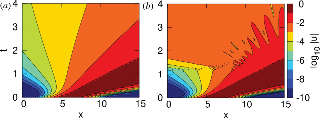
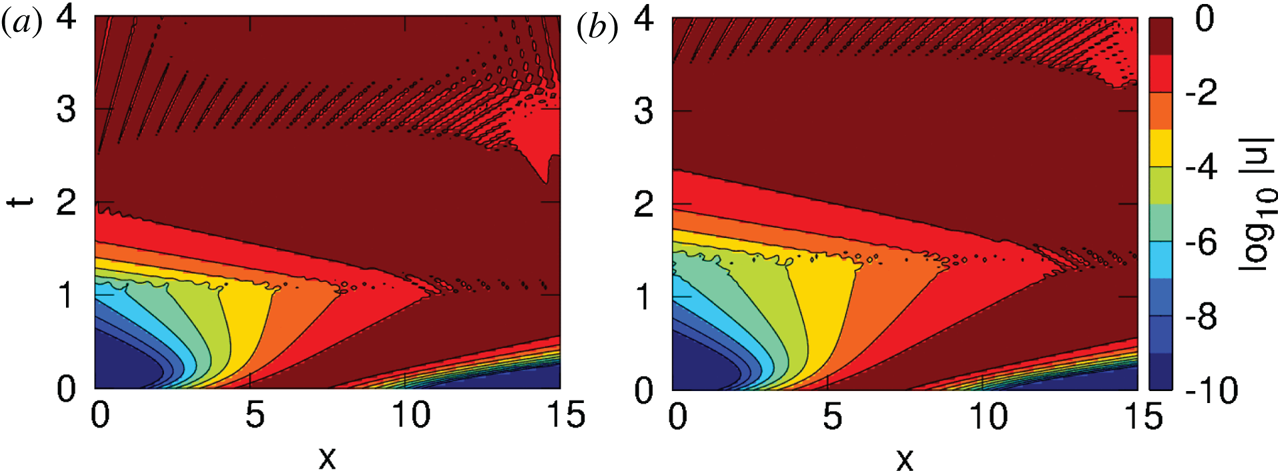
Figure 3 shows the density plot of  $\log _{10}|u (x, t) |$ (Antoine et al. Reference Antoine, Arnold, Besse and Schädle2008). Figure 3(a) traces the travelling Gaussian beam (2.10), i.e. the exact solution of the Schrödinger equation (2.1). At
 $t = 0$, the initial value of
 $u$ is almost confined in
 $[x_{{L}}, x_{{R}}]$ and
 $\log _{10}|u|$ is concentrated around the centre of the Gaussian beam,
 $x_{\textrm {c}} = 6$. The colour bands expand as time increases. Colour band borders are located at
 \begin{equation} \log_{10}|u| = n, \quad n \in \mathbb{Z}, \ -10 < n < 0, \end{equation}
e.g. lines between red and dark-red bands indicate  $\log _{10}|u| = -1$. After
 $t \approx 0.5$, the colour band borders are approximately straight in the domain under consideration. In the following analysis, we will focus on orange and red colour bands, i.e.
 $\log _{10}|u| \geq -3$.


Figure 3(b) shows the simulation result of the damping layer equation (4.2) with  $\sigma _0 = 40$. For
 $t < 1$, the colour bands are as smooth as for the exact solution. After
 $t = 1.2$, colour band borders become distorted by reflected waves, with a slight distortion at
 $\log _{10}|u| = -1$ and much stronger ones for smaller values of
 $\log _{10}|u|$. We can see that for the damping layer equation (4.2) with the widths
 $D_{{L}} = D_{{R}} = 2$, there is a large numerical error for
 $\log _{10}|u| < -2$. Changing the value of
 $\sigma _0$ does not significantly improve the situation. Making the boundary layer wider would reduce the error, but with a potentially large increase in the computational cost. To reduce the error without a significant increase in the computational cost, we would need to modify the boundary layer equation itself.
We now explore some approaches which could improve the damping layer equation (4.2). We consider that the waves in the Schrödinger equation move with phase velocity  $v_{\textrm {ph}} = k$, which means that waves with high wavenumber
 $k$ spend less time in the damping layer. Because the amount of damping for the dispersion relation (4.1) is constant per unit time, these fast waves will be only weakly damped, potentially resulting in large numerical errors. Therefore, we consider alternative dispersion relations that may be able to eliminate or reduce this problem.
Since the damping rate linearly proportional to  $k$ introduces an amplification of the left-propagating wave, we consider the dispersion relation
 \begin{equation} \omega = k^2 - \textrm{i} k^2 \sigma. \end{equation}
With this relation, waves will be damped in proportion to  $k^2$, and the corresponding Schrödinger equation becomes
 \begin{equation} \textrm{i} \partial_t u + (1 - \textrm{i} \sigma) \partial_x^2 u = 0. \end{equation}
By taking the terms with the imaginary unit, the new term looks like a diffusion term. Therefore, this damping layer equation damps waves through a diffusion effect. Since the damping effect proportional to  $k^2$ will work more efficiently for higher wavenumber waves, (4.9) may reduce the amplitude of waves more strongly than that of (4.2). To our knowledge, such a wavenumber-dependent damping has not been considered before.
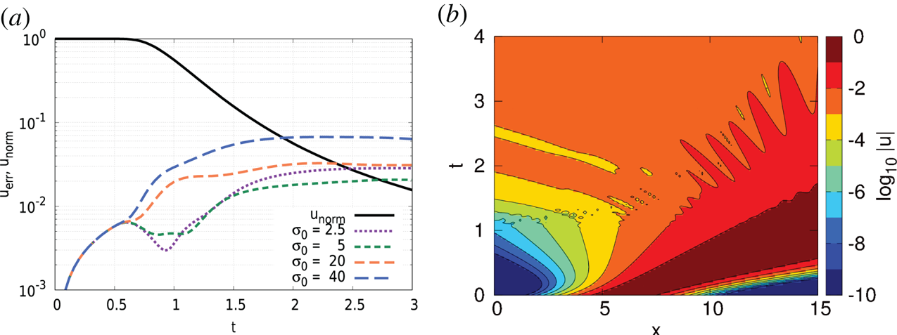
Figure 4 shows the numerical errors of simulation of the damping layer equation (4.9) in  $[x_{{L}}, x_{{R}}] = [0, 15]$ with the layer width
 $D_{{L}} = D_{{R}} = 2$. From the green dashed curve (
 $\sigma _0 = 5$) on figure 4(a), we can see that the crossover point with the black curve is around
 $t \approx 2.7$, with the numerical error
 $u_{\textrm {err}} \approx 0.02$. These values are similar to the blue dashed curve in figure 2 for the damping layer equation (4.2) with the damping function maximum
 $\sigma _0 = 40$.
Simulation results of the damping layer equation (4.9),  $D_{{L}} = D_{{R}} = 2$. (a) Numerical errors; (b) log contour plot,
 $\sigma _0 = 5$.

We may roughly compare the damping effects of the layer equations (4.2) and (4.9) to quantify their effectiveness. From (4.3) we obtain the damping rate  $R_{S}$ for the original damping layer equation (4.2), and analogously the damping rate
 $R_{S2}$ of the modified equation (4.9),
 \begin{equation} R_{S} = \sigma, \quad R_{S2} = k^2 \sigma. \end{equation}
By setting the wavenumber for  $R_{S2}$ to the peak of the Gaussian beam,
 $k = k_0$, we can make the rough estimate of the damping effects,
 $\tilde {R}_{S}$ and
 $\tilde {R}_{S2}$, as
 \begin{equation} \tilde{R}_{S} = 40, \quad \tilde{R}_{S2} = 5^2 \cdot 5 = 50, \end{equation}
where we have taken the maximum value  $\sigma _0$ for
 $\sigma$. In figure 4(a),
 $u_{\textrm {err}}$ becomes comparable for a smaller value of
 $\sigma _{0}$ compared with figure 2 due to the factor
 $k^2$ appearing in the
 $R_{S2}$ in (4.10a,b). However, for an even smaller value such as
 $\sigma _{0} = 2.5$ (purple dashed curve), the layer does not have a sufficient damping effect as is deduced from (4.10a,b), therefore,
 $u_{\textrm {err}}$ is larger than that of
 $\sigma _{0} = 5$ at
 $t = 3$.
Here, we suggested the second-order damping proportional to  $k^2$. We may also think of other higher-order damping (
 $k^{2m}$;
 $m \in \mathbb {N}$,
 $m \geq 2$); however, we do not consider it here since the corresponding higher-order derivative (
 $\partial _x^{2m} u$) introduces a larger bandwidth of the matrix in our numerical scheme.
Since  $\tilde {R}_{S} \simeq \tilde {R}_{S2}$, and comparing figures 3 and 4, we can see that neither of the damping layer equations (4.2) and (4.9) has a clearly superior performance. Therefore, we will consider a different approach in the next section.
4.2 Deceleration layers
In this section, we again start from modifying the dispersion relation (2.3).
First, we consider
 \begin{equation} \omega = \frac{k^2}{1 + \delta}, \end{equation}
where  $\delta$ is a positive real constant. The corresponding Schrödinger equation yields
 \begin{equation} \textrm{i} (1 + \delta)\partial_t u + \partial_x^2 u = 0. \end{equation}
To analyse the effect of  $\delta$, we repeat the procedure in (2.2) and (4.3). Assuming (2.2), we let
 $\hat {u}(x, t)$ be the solution of the original Schrödinger equation (2.1). Then we obtain the solution of (4.13) as
 \begin{equation} u(x, t) = \hat{u} \left(x, \frac{t}{1 + \delta} \right). \end{equation}
From the dispersion relation (2.3) and (4.12), we can obtain the phase velocities of the original Schrödinger equation (2.1) and the deceleration layer equation (4.13), respectively,
 \begin{equation} v_{\textrm{ph}}^{(2.1)} = k, \quad v_{\textrm{ph}}^{(4.13)} = \frac{k}{1 + \delta}. \end{equation}
We can see that the phase velocity of the wavefunction in (4.13) is slowed down by the factor  $1+\delta$, for
 $\delta > 0$. From (4.15a,b), we obtain the ratio of deceleration,
 \begin{equation} R_{D} = \frac{v_{\textrm{ph}}^{(2.1)} - v_{\textrm{ph}}^{(4.13)}}{v_{\textrm{ph}}^{(2.1)}} = 1 - \frac{1}{1 + \delta} = \frac{\delta}{1 + \delta}. \end{equation}
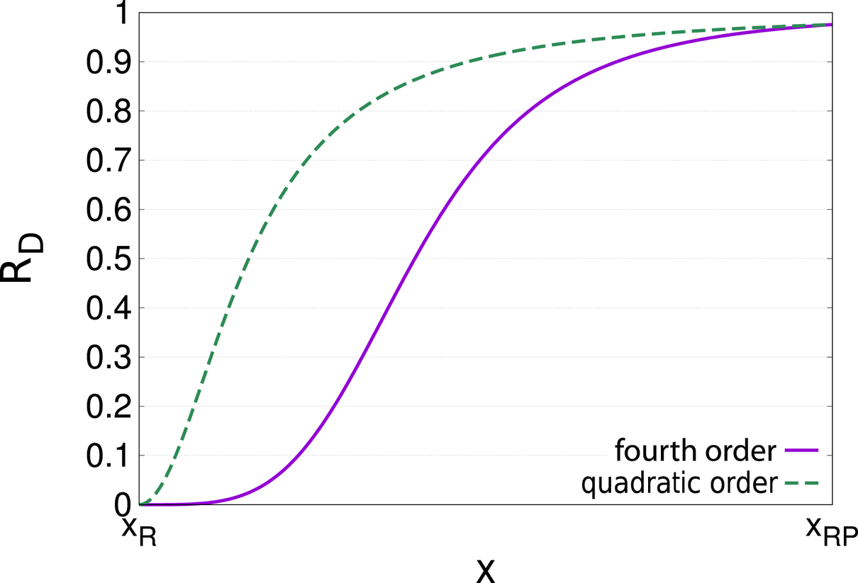
Thus, we will call  $\delta$ and the modified Schrödinger equation (4.13) the deceleration factor and the deceleration layer equation, respectively. As we described in § 3, the coordinate stretching (Zheng Reference Zheng2007) includes deceleration effects implicitly; however, to our knowledge, it has not been explicitly mentioned before.
Now we allow the spatial variation of  $\delta$ in the WKB sense (
 $k D_{R} \gg 1$) as in § 4.1, and show in figure 5 the ratio of deceleration
 $R_{D}$ in the boundary layer
 $(x_{{R}}, x_{\textrm {RP}}]$ for deceleration functions
 $\delta (x) = \delta _0 ((x - x_{{R}}) / D_{{R}})^4$ and
 $\delta = \delta _0 ((x - x_{{R}}) / D_{{R}})^2$. We can see that the former shows a gradual change over the entire exterior region, while the latter is shifted fairly close to the interior boundary.Since the fourth-order function shows the smooth matching to the interior domain
 $[x_{{L}}, x_{{R}}]$ as in figure 5, we chose the fourth order and let
 $\delta$ be
 \begin{equation} \delta(x) = \begin{cases} \delta_0 \left( \dfrac{x - x_{{L}}}{D_{{L}}} \right)^4 & (x_{\textrm{LP}} \leq x < x_{{L}}), \\ 0 & (x_{{L}} \leq x \leq x_{{R}}), \\ \delta_0 \left( \dfrac{x - x_{{R}}}{D_{{R}}} \right)^4 & (x_{{R}} < x \leq x_{\textrm{RP}}), \end{cases} \end{equation}
where the constant  $\delta _0$ is the maximum value of
 $\delta (x)$ in
 $[x_{\textrm {LP}}, x_{\textrm {RP}}]$. It should be emphasized that
 $\delta (x)$ and
 $\delta _0$ do not directly indicate the maximum rate of deceleration, although
 $\delta (x)$ and
 $\delta _0$ are called deceleration function and its maximum hereafter. We note here that
 $\delta (x)$ and
 $\delta _0$ control the ratio of deceleration through (4.16). The expression for
 $\delta (x)$ is similar to the expression (4.4) for
 $\sigma (x)$, except that
 $\delta (x)$ is a fourth-order polynomial.
The comparison of deceleration effect with the fourth order  $\delta (x)$ and the quadratic
 $\delta (x)$.

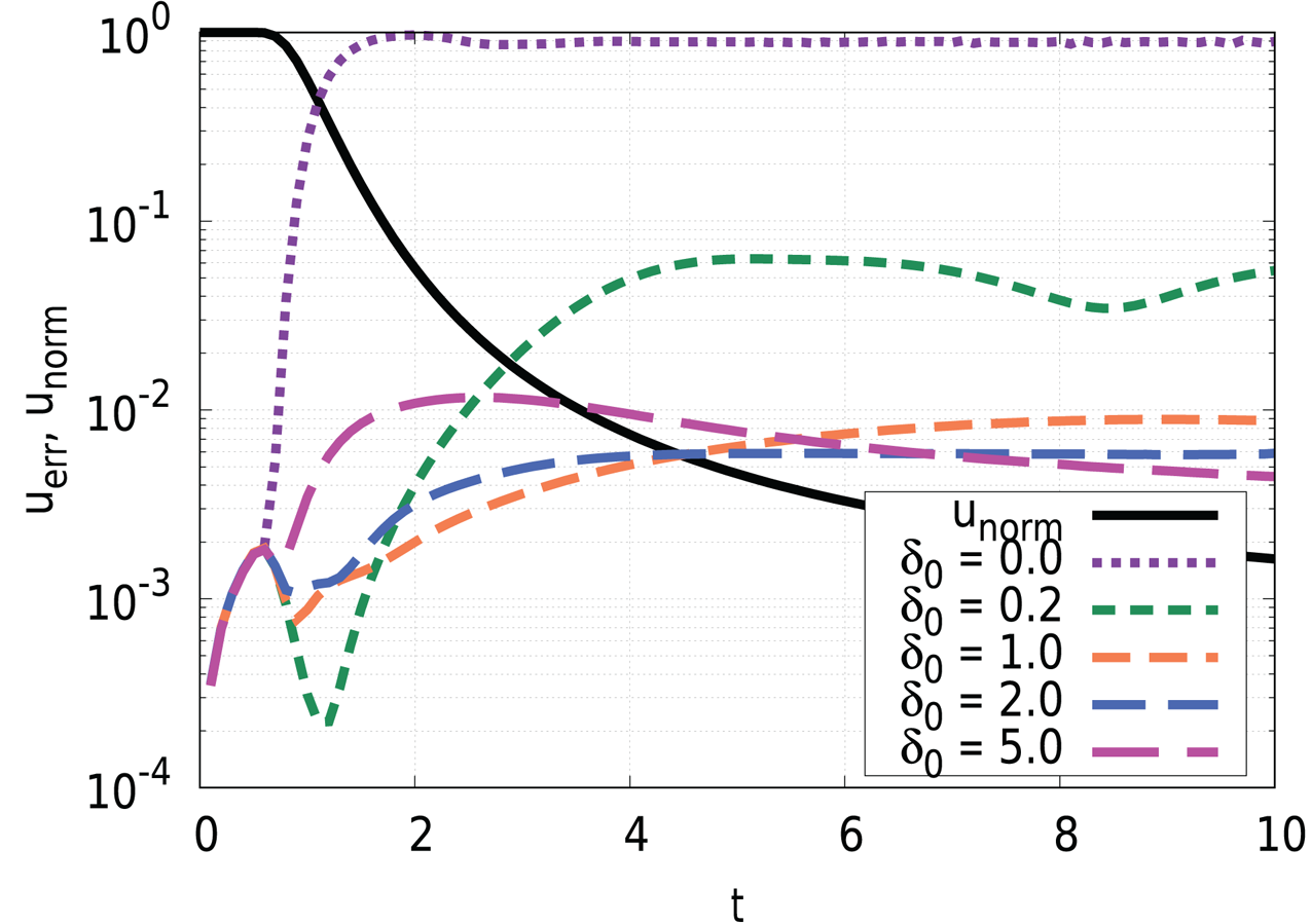
Similar to § 4.1, figure 6 depicts the numerical errors  $u_{\textrm {err}}$ of the simulation for the deceleration layer equation (4.13). Here we show the long-time evolution since it is instructive to compare with the conservation property of (4.13) later in (4.18). However, it is noted that the result is not desired for the purpose of applications when the numerical error becomes significantly larger than
 $u_{\textrm {norm}}$. Note also that this figure is shown with a linear scale. The purple dashed curve (
 $\delta _0 = 0$), where the deceleration layer does not actually decelerate, is used as a reference, while the other curves are for simulations with finite deceleration. Numerical error for
 $\delta _0 = 0$ starts increasing around
 $t \approx 0.7$, while those for
 $\delta _0 > 0$ are delayed, with the delay increasing as
 $\delta _0$ increases. Therefore, the development of the numerical errors is delayed by the deceleration layers. For
 $t \gtrsim 1$, all of the dashed curves in figure 6 increase by the reflected waves from the outer boundaries of the layers,
 $x_{\textrm {LP}}$ and
 $x_{\textrm {RP}}$.
Numerical errors of the deceleration layer equation (4.13),  $D_{{L}} = D_{{R}} = 2$. Note that this plot is shown with a linear scale.

At  $t > 2$, the error eventually rises up close to unity, which shows the fact that the bulk of the waves are reflected back to enter the interior domain. However, the saturated level at
 $t \gtrsim 4$ differs among the values of
 $\delta _0$, which is because of the broken invariant. The deceleration layer (4.13) is designed mainly to decelerate the waves, however, the inclusion of
 $\delta$ changes the conservation property (2.5). Now the conservation (2.5) is modified to
 \begin{equation} \partial_t \int_{\varOmega_{D}} (1+\delta) |u|^2 \, \textrm{d}x = 0, \end{equation}
which exactly holds for an arbitrary function  $\delta (x)$. In the case of
 $\delta _0 = 0$, one might think that the error should approach unity in the long time limit; however, it doesn't in figure 6. This is because we take the norm only in the interior region as shown in (4.5). When we change the norm to include the exterior region, the error actually approaches unity by
 $t \lesssim 3$ and stays there for the rest of simulation period (not shown). Since the waves are not decelerated for
 $\delta _0 = 0$, the waves go in and out of the exterior region, and some fraction of the waves are present in the exterior region all the time at
 $t \gtrsim 4$, which amounts to the difference of the purple dashed line (
 $\delta _0 = 0$) from unity.
Again similar to § 4.1, in figure 7 we have two density plots; panel (a) shows the result with no deceleration, while panel (b) shows the result for the maximum value of the deceleration function  $\delta _0 = 40$. For
 $t < 1$ in panel (a), the colour band borders are smooth, i.e. there are no reflected waves yet. For
 $t > 1$, the border at
 $\log _{10}|u| = -1$ completely changes direction due to the waves re-entering the interior domain
 $[x_{{L}}, x_{{R}}]$ after reflecting from the outer boundaries of the exterior domains at
 $x_{\textrm {LP}}$ and
 $x_{\textrm {RP}}$ due to the Dirichlet BCs (2.8). In figure 7(b), the colour band border at
 $\log _{10}|u| = -1$ also changes direction, though only for
 $t > 1.4$. Therefore, we can confirm the effects of the deceleration layer equation (4.13), even though the qualitative structure is unchanged.
Density plots of  $\log _{10}|u|$ for the deceleration layer equation (4.13) with the boundary layer thickness
 $D_{{L}} = D_{{R}} = 2$. (a)
 $\delta _0 = 0$ (no deceleration); (b)
 $\delta _0 = 40$.

Continuing the approach from § 4.1 on the damping layers, waves with high wavenumbers will pass through the deceleration layers faster. Since the deceleration ratio is constant per unit time, this means they will be decelerated by a smaller amount. We repeat the procedure from § 4.1 and consider alternative dispersion relations so that the ratio of deceleration will increase for larger wavenumbers.
Since the deceleration effect proportional to  $k$ introduces an acceleration of left-propagating waves, we suggest the dispersion relation
 \begin{equation} \omega = \frac{k^2}{1 + k^2 \delta}. \end{equation}
As in § 3, the relation  $\omega < k^2$ with
 $k \in \mathbb {R}$ permits the deceleration for waves of the Schrödinger equation. By replacing the complex number
 $R$ in (3.16) with a real number
 $k^2$, we can focus on the pure deceleration without damping. Further, we expect that the deceleration with the factor
 $k^2$ will cancel out the dispersive effect of the Schrödinger equation.
The corresponding Schrödinger equation yields
 \begin{equation} \textrm{i} \partial_t (1 - \delta \partial_x^2) u + \partial_x^2 u = 0, \end{equation}
where the deceleration function  $\delta = \delta (x)$ is the same as (4.17). From the dispersion relation (4.19), the phase velocity of the Schrödinger equation (4.20) is
 \begin{equation} v_{\textrm{ph}}^{(4.20)} = \frac{k}{1 + k^2 \delta}. \end{equation}
Repeating the procedure we used to obtain (4.16), the ratio of the deceleration layer equation (4.20) becomes
 \begin{equation} R_{D2} = 1 - \frac{1}{1 + k^2 \delta} = \frac{k^2 \delta}{1 + k^2 \delta}. \end{equation}
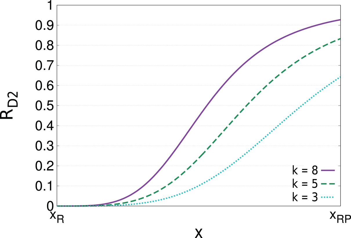
From (4.22), the ratio of deceleration increases with  $k^2$ and the comparison of deceleration effects with the wavenumber is shown in figure 8. We can see that the waves with larger wavenumbers slow down at an earlier stage than the waves with smaller wavenumbers. Furthermore, the relation means that deceleration is independent of wave direction, therefore the erroneous waves that travel in the wrong direction will also be decelerated. However, it should be noted that the left-travelling waves which appeared in the right-hand exterior region will eventually re-enter the interior domain since (4.20) is designed for deceleration and not for damping, which will be discussed later in more detail.
Comparison of the deceleration ratio  $R_{D2}$ for several wavenumbers.

Figure 9 depicts the numerical errors of the simulation for the new deceleration layer equation (4.20). Here we show the long-time evolution again in order to compare with the conservation property of (4.20). Similar to figure 6, the purple dashed curve ( $\delta _{0} = 0$) is a reference with no deceleration, while the others have active deceleration layers. Due to the more powerful deceleration effect in the layers, the deceleration layer equation (4.20) will compress waves more than the previous deceleration layer equation (4.13). This compression leads to the steep gradient of the field, thus, we applied a finer spatial step size for the simulation of (4.20), i.e.
 ${\rm \Delta} x = 10^{-3}$, except for the case with
 $\delta _0 = 5$ where we used the even smaller value of
 ${\rm \Delta} x = 5 \times 10^{-4}$ for convergence.
Numerical errors of the deceleration layer equation (4.20),  $D_{{L}} = D_{{R}} = 2$.

The purple dashed curve ( $\delta _0 = 0$) reaches the peak numerical error
 $u_{\textrm {err}} \approx 1$ very early, at
 $t \approx 1.7$, while the green dashed curve (
 $\delta _0 = 0.2$) reaches close to the (lower) peak much later, at
 $t \approx 5$. Therefore, the deceleration layer with
 $\delta _0 = 0.2$ slowed down the reflected waves by approximately three times. This result indicates that the new deceleration layer (4.20) is more efficient for the Schrödinger equation (2.1) than the deceleration layer (4.13), i.e. we can expect that the dependence of the deceleration effect on wavenumber
 $k$ may improve our approximation. While the errors at the later stage (
 $t \gtrsim 6$) decrease as
 $\delta _0$ increases, the errors at the early stage increase for larger
 $\delta _0$. This is because of the reflection by the too strong deceleration. Even though the deceleration effect does not make the phase speed of the waves precisely zero, the waves will be reflected before they reach the right-hand end of the deceleration layer when the deceleration function changes rapidly for large
 $\delta _0$. It is also noted here that the levels of numerical errors at
 $t \gtrsim 4$ saturate at significantly lower levels than unity. This is again because of the broken invariant as in the case of figure 6. Equation (4.20) changes the conservation property (2.5) into
 \begin{equation} \partial_t \int_{\varOmega_{D}} |u - \delta \partial_x^2 u|^2 \, \textrm{d}x = 0,\end{equation}
which again holds exactly for a spatially varying  $\delta (x)$. Unlike (4.18),
 $u$ is coupled with
 $\partial _x^2 u$ in (4.23), and thus, we cannot tell much about the behaviour of
 $||u||$ from (4.23). On the other hand, we can show that
 \begin{equation} \partial_t \int (|u|^2 + \delta |\partial_x u|^2) \, \textrm{d}x \approx 0 \end{equation}
holds approximately in the WKB sense. This implies that the wave amplitude  $||u||$ may be reduced by the generation of
 $||\partial _x u||$, which actually takes place by the wave compression mentioned earlier.
Since the deceleration model (4.20) reduces the amplitude but introduces the steep gradient due to wave compression, the damping effect will be added on the deceleration layer to improve our approximation in § 4.3.
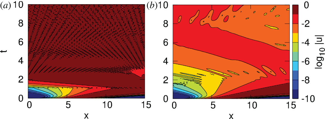
In figure 10, we again compare a plot with a disabled deceleration layer and a plot with an active deceleration layer, to confirm what is the actual improvement in numerical reflections. Here the time scale is extended to match figure 9. Figure 10(a) corresponds to the case with no deceleration, and shows that the fluctuation that exceeds  $|u| > 0.1$ (dark red) spreads over the whole domain at
 $t \gtrsim 2$ due to wave dispersion. In figure 10(b) which corresponds to
 $\delta _0 = 0.2$, the fluctuation of
 $|u| > 0.1$ (dark red) has successfully gone out of the interior region; however, that of
 $10^{-2} < |u| < 0.1$ (bright red) is reflected around
 $t \approx 4$ in the right-hand exterior region, and travels back and forth thereafter. Looking at the earlier stage, we can see that the colour band border at
 $\log _{10}|u| = -1$ shows no oscillation until
 $t = 1.7$ where it reaches the right-hand boundary
 $x = 15$. Although the reflections from smaller fluctuations re-enter the interior domain before that, this boundary layer will be very useful in constructing the absorbing layer in the following section.
Density plots of  $\log _{10}|u|$ for the deceleration layer equation (4.20) with the boundary layer thickness
 $D_{{L}} = D_{{R}} = 2$. (a)
 $\delta _0 = 0$ (no deceleration); (b)
 $\delta _0 = 0.20$.

4.3 Absorbing layer
In §§ 4.1 and 4.2 we introduced the damping and the deceleration layers. In this section we will combine those layers into a compound layer. Since we introduced two useful types of each layer, damping layers (4.2) and (4.9), and deceleration layers (4.13) and (4.20), there is a total of four possible layer combinations with both damping and deceleration effects. In this paper we focus on the fictitious absorbing layer
 \begin{equation} \textrm{i} \partial_t (1 - \delta \partial_x^2) u + (1 - \textrm{i} \sigma \delta) \partial_x^2 u + \textrm{i} \sigma u = 0, \end{equation}
which is obtained by combining the damping layer (4.2) with the deceleration layer (4.20). This combination has shown to be the most suitable one, for reasons explained below.
First, the analysis in § 4.1 showed that there is no significant difference between the optimal error levels of the damping layers (4.2) and (4.9), so either one should be acceptable. Next, the analysis in § 4.2 showed that the deceleration layer (4.20) delays waves more effectively than the deceleration layer (4.13); we expect that the same holds for the combined absorption layers constructed from them. Finally, when combining the damping layers (4.2) and (4.9) with deceleration layer (4.20), the combination with (4.9) might include a fourth derivative. One might think that the combination of (4.9) and (4.20) may yield
 \begin{equation} \textrm{i} \partial_t (1 - \delta \partial_x^2) u + (1 - \textrm{i} \sigma) \partial_x^2 u = 0, \end{equation}
however, this will bring about a damping rate independent of  $k$ in the large
 $k$ limit. In order to achieve the damping rate proportional to
 $k^2$ in the large
 $k$ limit, we would have to invoke the fourth-order derivative. Since the fourth-order derivative would increase the bandwidth of the matrix in our numerical scheme, we choose the combination with (4.2), as it offers comparable effectiveness for less complexity.
The dispersion relation of the absorbing layer equation (4.25) is
 \begin{equation} \omega = \frac{k^2}{1 + k^2 \delta} - \textrm{i} \sigma. \end{equation}
The absorbing layer equation (4.25), which has the effect of the damping layer equation (4.2), as well as the effect of the deceleration layer equation (4.20), was obtained from (4.27) by a procedure similar to those in §§ 4.1 and 4.2. To confirm the damping and deceleration effects of this equation, we again employ the same two types of plots as before. In this section, we use  ${\rm \Delta} x = 10^{-3}$, as in § 4.2, since we need to resolve the sharp gradient due to compressed waves.
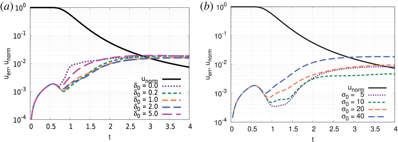
Figure 11(a) shows the numerical errors with variable maximum values of the deceleration function,  $\delta _0$, and a fixed damping function maximum (
 $\sigma _0 = 40$), which showed the best result in earlier tests. We note here again that the deceleration function
 $\delta (x)$ does not directly indicate the rate of deceleration; however, it controls the ratio of deceleration through (4.16). Comparing the purple dashed curve (no deceleration) with others (with deceleration), the former reaches the numerical error
 $u_{\textrm {err}} = 0.01$ around
 $t \approx 1.2$, while the latter does around
 $t \approx 2.0$ except for the case with
 $\delta _0 = 5$ around
 $t \approx 1.5$. Thus, we have confirmed that the absorbing layer (4.25) can delay the numerical errors by the deceleration effect; however, too strong deceleration (
 $\delta _0 = 5$) yields large numerical errors at the early stage. The difference of the error level between the purple dashed curve and the others around
 $t \geq 3$ is not significant. Therefore, modifying only the deceleration factor while keeping the damping factor fixed does not have much impact in the long-time limit.
Numerical errors of the absorbing layer equation (4.25) with the layer thickness  $D_{{L}} = D_{{R}} = 2$. (a) Variable maximum value of the deceleration function
 $\delta _0$ with fixed damping function maximum
 $\sigma _0 = 40$, which was the best parameter in the simulation for the damping layer equation (4.2) in figure 2. (b) Variable damping function maximum
 $\sigma _0$ with fixed maximum value of the deceleration function
 $\delta _0 = 0.2$.

Figure 11(b) shows the numerical errors with variable damping function maximum and a fixed maximum value of the deceleration function ( $\delta _0 = 0.2$). At
 $t = 4$, the numerical error for
 $\sigma _0 = 10$ (the green dashed curve) shows
 $u_{\textrm {err}} < 0.01$ unlike the other curves. Decreasing
 $\sigma _0$ from 40 to 10 reduced the steepness of the damping function, which resulted in fewer early reflections. At the same time, the deceleration effect made the waves spend more time inside of the absorbing layer, which compensated for the weaker damping effect and resulted in more damping. However, for
 $t = 4$, the purple dashed curve (
 $\sigma _{0} = 5$) shows larger errors than the green dashed curve (
 $\sigma _{0} = 10$). This fact shows that sufficient amount of damping is required even for the decelerated waves. The two effects of damping and deceleration need to be balanced carefully for a good approximation of this absorbing layer. The cumulative effects of damping and deceleration reduced the numerical error at
 $t = 4$ to order
 $10^{-2}$, a significantly stronger absorbing effect than either of the layers could provide in isolation.
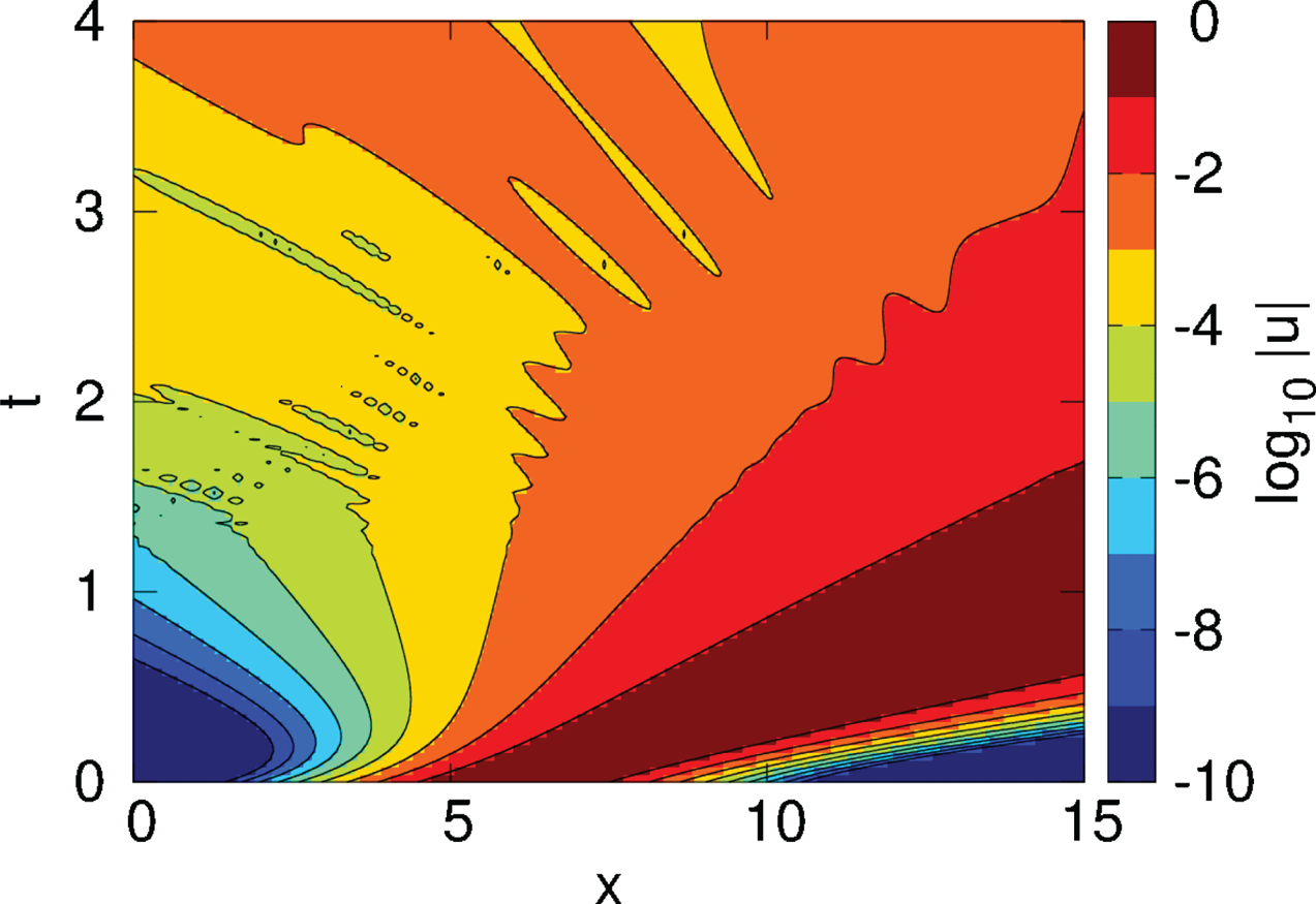
Figure 12 shows the result with the most suitable parameters from figure 11, i.e. model (4.25) with  $\sigma _0 = 10$ in (4.4) and
 $\delta _0 = 0.2$ in (4.17). As the absorbing layer equation (4.25) brings about the deceleration effect of the deceleration layer equation (4.20), the onset of oscillations of the colour band borders should be suppressed in a similar manner. Comparing the colour band border at
 $\log _{10}|u| = -1$ in figures 12 and 10(b), we can see that in both of them these lines show no oscillation until
 $t = 1.7$ where they reach the right-hand boundary
 $x=15$, confirming the deceleration effect. However, in figure 10(b), the colour band border at
 $\log _{10}|u| = -2$ starts to show oscillations around
 $t \approx 1.7$, while the same border in figure 12 shows some tiny oscillations somewhat earlier, around
 $t \approx 1.4$. On the other hand, the overall orientation of this border does not change in figure 12 up until
 $t \approx 3.5$, while that in figure 10 changes direction to the left around
 $t \approx 2.3$.
Density plot of  $\log _{10}|u|$ for the absorbing layer equation (4.25) with the boundary layer thickness
 $D_{{L}} = D_{{R}} = 2$. The damping function maximum is
 $\sigma _0 = 10$, and the maximum value of the deceleration function is
 $\delta _0 = 0.2$.

So far we have evaluated the effectiveness of the absorbing layer equation (4.25) for a Gaussian beam with a singly peaked wavenumber. However, in practical applications, the wave spectrum which approaches the boundary may be more complex. Thus we investigate the case of multiple waves with different group velocity as the initial condition for the absorbing layer equation (4.25).
Before using the complex wave spectrum, we first show the results for three independent Gaussian beams with variable peak wavenumbers. For the initial value we fixed the centre of each Gaussian beam to  $x_{\textrm {c}} = 0$ and set the interior domain to
 $[x_{{L}}, x_{{R}}] = [-10, 10]$.
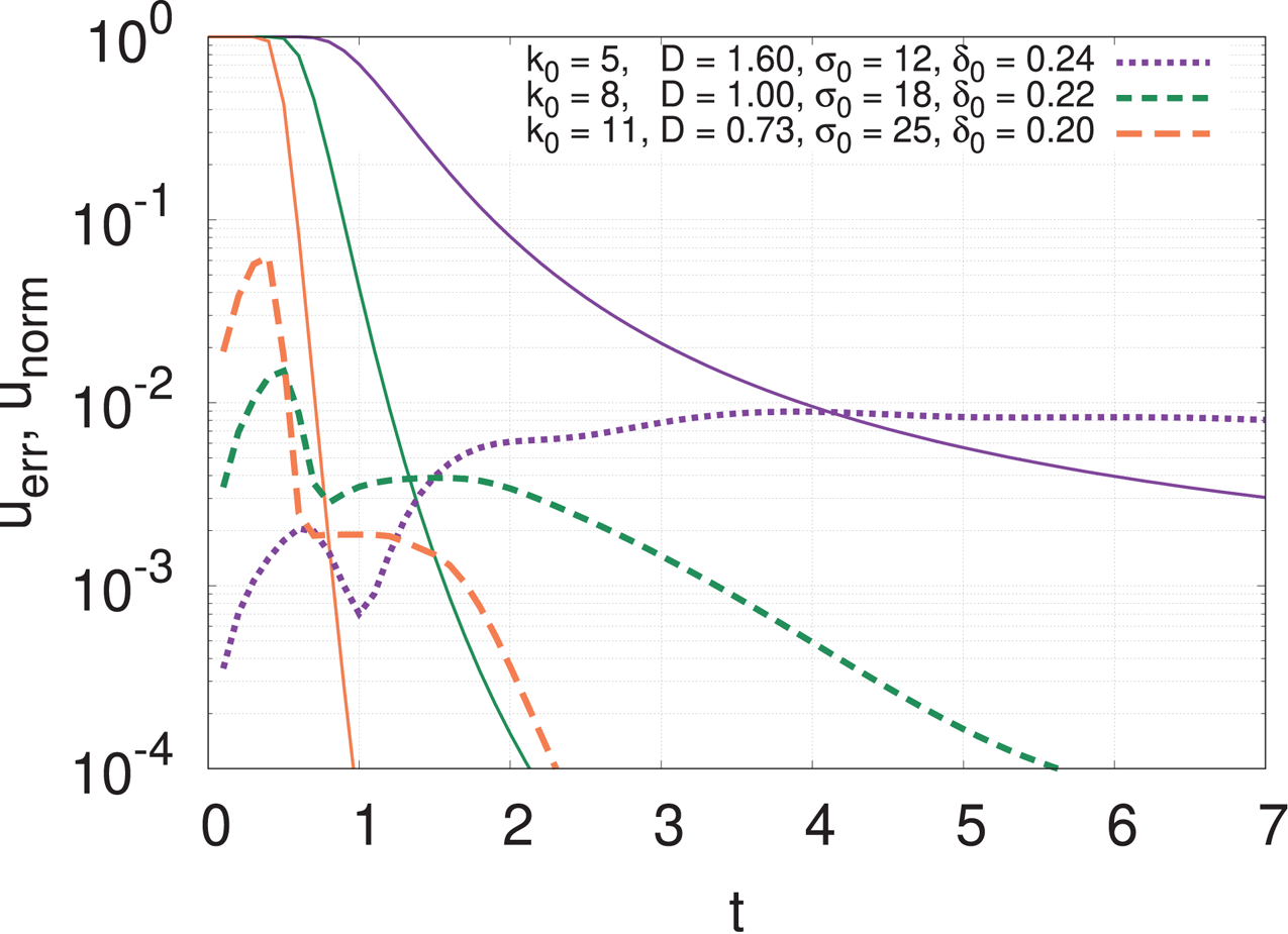
Figure 13 depicts the numerical errors for variable peak wavenumbers ( $k_{0} = 5$,
 $8$ and
 $11$). In order to keep the accuracy of the WKB approximation by
 $k D = 8$, we set the layer width to
 $D = 1.6$ for waves with peak wavenumber
 $k_{0} = 5$, to
 $D = 8$ for
 $k_{0} = 8$, and to
 $D = 0.73$ for
 $k_{0} = 11$, where we chose the optimal
 $\sigma _{0}$ and
 $\delta _{0}$ to minimize the
 $u_{\textrm {err}}$ for each case. Solid and dashed curves in figure 13 indicate
 $u_{\textrm {norm}}$ (4.6) and
 $u_{\textrm {err}}$ (4.5), respectively. Purple curves correspond to the smallest phase velocity wave (
 $k_{0} =5$), thus, its
 $u_{\textrm {norm}}$ (solid purple curve) shows the slowest decrease. In this case, the numerical error becomes stationary at
 $u_{\textrm {err}} = 0.00836$ around
 $t \simeq 5$. For orange curves (
 $k_{0} = 11$), due to their largest phase velocity, the numerical error becomes stationary earlier around
 $t \simeq 1$ at
 $u_{\textrm {err}} = 0.00190$. Waves with higher peak wavenumber (i.e. finer structure) are damped more strongly; therefore, the absorbing layer performs more effectively for them.
Numerical errors of the absorbing layer equation (4.25) with  $k D = 8$.

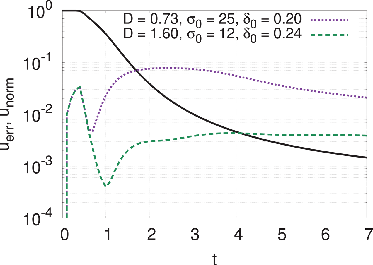
Next as an example of the complex wave spectrum, we use the three preceding Gaussian beams superimposed with the same amplitude. Figure 14 depicts numerical errors of the simulations for an initial condition with the superposition of three Gaussian beams with the peak wavenumbers  $k_{0} = 5$,
 $8$ and
 $11$. The purple (green) curve uses the parameters
 $D$,
 $\sigma _{0}$ and
 $\delta _{0}$ adjusted for the single Gaussian beam of
 $k_{0} = 11$ (
 $k_{0}=5$) in figure 13. It is shown by the large error of the purple curve that the absorbing layer with parameters adjusted for the high wavenumber (
 $k_{0} = 11$) could not sufficiently absorb low wavenumber components. By the time
 $t \lesssim 3$, the error
 $u_{\textrm {err}}$ becomes stationary with a value above
 $10^{-2}$. It is noted that we ignored the decrease in
 $t > 3$ since this corresponds to the period when the reflected waves entered the left-hand exterior region. In contrast, the error
 $u_{\textrm {err}}$ of the green curve becomes stationary at
 $t \gtrsim 3.5$ with the value between those of
 $k_{0} =5$ and
 $11$ in figure 13. Therefore, the absorbing layer with parameters adjusted for the lowest peak wavenumber shows effective absorption for waves with multiple peak wavenumbers.
Numerical errors of the absorbing layer equation (4.25) with initial condition with three peak wavenumbers ( $k_{0} = 5, 8, 11$).

5 Application to nonlinear problems
In § 4.3, the absorbing layer equation (4.25) showed its effectiveness for linear problems. In this section, we use a nonlinear Schrödinger equation with real-valued potential function  $V (x, t, |u|^2)$,
 \begin{equation} \textrm{i} \partial_t u + \partial_x^2 u = V(x, t, |u|^2) u. \end{equation}
The nonlinear Schrödinger equation that includes a cubic nonlinear term corresponding to the potential
 \begin{equation} V(x, t, |u|^2) = - 2 |u|^2, \end{equation}
admits the soliton solution (Zheng Reference Zheng2007)
 \begin{equation} u_{\textrm{Nex}} = \sqrt{a} \, \textrm{sech} [ \sqrt{a} (x - ct)] \exp\left({ \textrm{i} \left[ \frac{c}{2} x + \left( a - \frac{c^2}{4} \right) t \right] }\right), \end{equation}
with the initial value
 \begin{equation} u_{\textrm{Ninit}} = \sqrt{a} \,\textrm{sech} ( \sqrt{a} x ) \exp\left({ \textrm{i} \left( \frac{c}{2} x \right) }\right), \end{equation}
where  $a$ and
 $c$ are real constants. The soliton solution (5.3) consists of an envelope wave
 $|u|$ with characteristic width
 $1 / \sqrt {a}$ and a carrier wave
 $\exp \{ \textrm {i} [ ({c}/{2}) x + ( a - ({c^2}/{4}) ) t ] \}$ with wavenumber
 $c / 2$. In the finite domain
 $\varOmega _{D}$ (4.12), this equation also satisfies the normalization condition (2.5) under the Dirichlet BC (2.8). As with the linear Schrödinger equation, therefore, we use a central finite difference method for spatial discretization with the CN method for time integration. The wavefunction
 $u$ from the nonlinear Schrödinger equation with these discretization methods satisfies (2.5); however, the use of the implicit CN method is not trivial for nonlinear problems. We now split (5.1) into a nonlinear part
 \begin{equation} \textrm{i} \partial_t u = V(x, t, |u|^2) u \end{equation}
and a linear part
 \begin{equation} \textrm{i} \partial_t u + \partial_x^2 u = 0. \end{equation}
Since the nonlinear part conserves  $|u|$ locally, the use of Strang splitting (LeVeque Reference LeVeque1992; Strang Reference Strang1968) yields
 \begin{gather} u^{(\star)}= u^{(n)} \exp \left[ - \frac{\textrm{i} {\rm \Delta} t}{2} V^{(n)} \right], \end{gather}
 \begin{gather}\frac{ u^{(\star\star)} - u^{(\star)} }{{\rm \Delta} t}= \frac{\textrm{i}}{2} \left[ \partial_x^2 u^{(\star)} + \partial_x^2 u^{(\star\star)} \right], \end{gather}
 \begin{gather}u^{(n+1)} = u^{(\star\star)} \exp \left[ - \frac{\textrm{i} {\rm \Delta} t}{2} V^{(\star\star)} \right], \end{gather}
by which we achieve the second-order accuracy and invariance of the norm.
In order to implement the absorbing layer in the nonlinear equation (5.1), we may only replace its linear part (5.6) by the absorbing layer equation (4.25), and now we obtain
 \begin{equation} \left.\begin{array}{c@{}} \textrm{i} \partial_t u = V (x, t, |u|^2) u, \\ \textrm{i} \partial_t (1 - \delta \partial_x^2) u + (1 - \textrm{i} \sigma \delta) \partial_x^2 u + \textrm{i} \sigma u = 0, \end{array}\right\}\end{equation}
where  $\delta$ and
 $\sigma$ denote the deceleration function (4.17) and damping function (4.4), respectively. In this section, we compute the layer equation (5.10), and apply the splitting scheme (5.7), (5.8), (5.9) with
 ${\rm \Delta} x = {\rm \Delta} t = 10^{-3}$. We set the interior domain to
 $[x_{{L}}, x_{{R}}] = [-10, 10]$ with the layer thickness
 $D_{{L}} = D_{{R}} = 1$. For the initial value we use the soliton solution (5.4) with
 $a = 2$ and
 $c = 16$. In order to evaluate the accuracy of the approximation, we estimate the error
 $u_{\textrm {err}}$ (4.5) and the norm
 $u_{\textrm {norm}}$ (4.6) as in § 4.3.
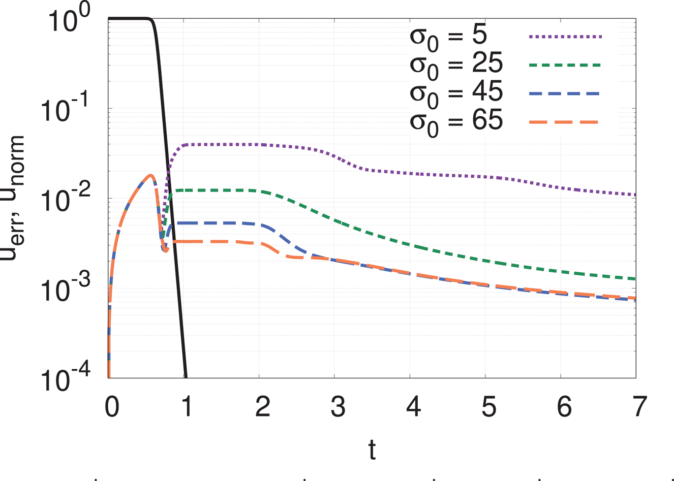
Figure 15 shows the results for the absorbing layer equation (5.10) with the fixed maximum value of the deceleration function  $\delta _0 = 0.04$ and variable damping function maximum,
 $\sigma _0$. Since the envelope of the soliton solution
 $|u|$ travels at a constant velocity
 $c$ without changing its form,
 $u_{\textrm {norm}}$ (black curve) falls down straightforwardly in
 $0.7 < t < 1.1$. At the time when numerical errors become stationary (i.e.
 $t = 1.4$),
 $\sigma _{0} = 65$ gives the smallest error,
 $u_{\textrm {err}} = 0.00330$.
Numerical errors of the absorbing layer equation (5.10) with the layer thickness  $D_{{L}} = D_{{R}} = 1$. Variable damping function maximum
 $\sigma _{0}$ with fixed maximum value of the deceleration function
 $\delta _{0} = 0.04$.

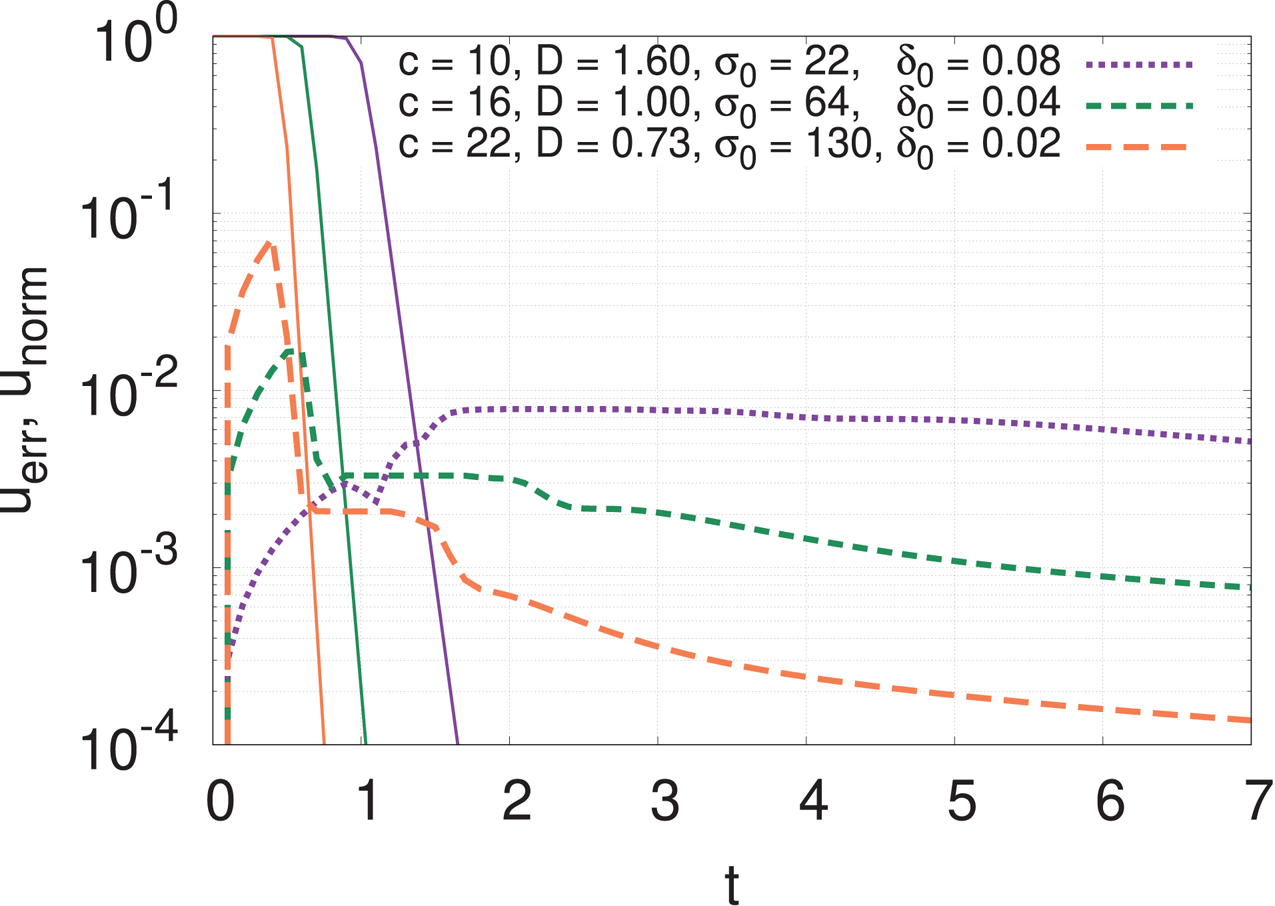
In figure 16, we evaluated the norm  $u_{\textrm {norm}}$ and the error
 $u_{\textrm {err}}$ for three independent solitons (5.3) with propagation velocities
 $c = 10$,
 $16$ and
 $22$. When the characteristic width of the envelope
 $|u|$ is larger than the wavelength of the carrier, i.e.
 $\sqrt {a} \ll c / 2$, the wavenumber
 $c/2$ of the carrier part corresponds to
 $k_{0}$ of Gaussian beam (2.10). Thus, we chose the layer width
 $D$ for each velocity to satisfy
 $c D / 2 = 8$. The amplitude of all solitons are
 $\sqrt {a} = \sqrt {2}$ and other parameters are the same as in § 4.3 except for the initial condition. Similarly to the linear problem, a high group velocity
 $c = 22$ (orange curve) gives the smallest numerical error (
 $t \simeq 1.0$). Conversely, the numerical error for the low group velocity
 $c = 10$ (purple curve) shows a value larger than the other cases at the stationary time
 $t \simeq 2.0$.
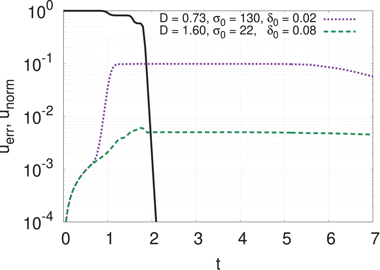
Numerical errors of the absorbing layer equation (5.10) with  $k D = 8$.

Figure 17 depicts numerical errors of a simulation with three solitons superimposed with the same amplitude and with different group velocities ( $c = 10$,
 $16$ and
 $22$). In order to prevent interferences between the solitons, we rewrite the soliton solution (5.3) as
 \begin{equation} u_{\textrm{Nex}} = \sqrt{a} \,\textrm{sech} [ \sqrt{a} (x - x_{{s}} - ct)] \exp\left({ \textrm{i} \left[ \frac{c}{2} (x - x_{{s}}) + \left( a - \frac{c^2}{4} \right) t \right] }\right), \end{equation}
where  $x_{{s}}$ is the initial position of the centre of soliton, and sufficiently separate their initial positions. We set the first soliton with
 $c = 22$,
 $x_{{s}} = -15$, the second one with
 $c = 16$,
 $x_{{s}} = 0$, and the third one with
 $c = 10$,
 $x_{{s}} = 15$, in the interior domain
 $[x_{{L}}, x_{{R}}] = [-25, 25]$, so that they all reach the right-hand boundary in a short period of
 $1 \lesssim t \lesssim 2$. Note that the performance of the absorbing layer in this paper does not depend on the domain size or initial positions as long as the initial value is in the interior domain. In order to reduce the discretization error for
 $t < 1$, we set the grid size
 ${\rm \Delta} x = 10^{-3}$ and
 ${\rm \Delta} t = 10^{-4}$. In figure 17, the numerical norm (4.6) of the total solitons (the black curve) decreases in three stages. First at
 $t \simeq 1.0$, the first soliton
 $c = 10$ goes out of the interior domain. For
 $t \simeq 1.6$ and
 $1.8$, the other solitons with
 $c = 16$ and
 $22$ follow. The purple (green) curve has the parameters
 $D$,
 $\sigma _{0}$ and
 $\delta _{0}$ adjusted for a soliton with group velocity
 $c = 22$ (
 $c = 10$) in figure 16. Similar to the linear problem in figure 14, the absorbing layer with corresponding parameter for a long wavelength wave (i.e. low wavenumber) damped out multiple solitons more effectively than the layer adjusted for a short wavelength wave.
Numerical errors of the absorbing layer equation (5.10) for three solitons superimposed.

6 Conclusion
We extended the idea of Berenger's PML (Berenger Reference Berenger1994) into an absorbing boundary layer with multiple effects for linear and nonlinear Schrödinger equations, which has shown an improved ability to reduce errors in the simulation. We expect that widening the absorbing layer could further reduce the errors, although it would also increase the computational cost.
We reviewed the complex coordinate transform (3.1), which was first introduced for wave equations by Chew & Weedon (Reference Chew and Weedon1994) and later imported to the Schrödinger equation by Zheng (Reference Zheng2007). Since this transform has multiple effects, damping and deceleration, we proposed to split and use them independently based on the WKB formalism, which added flexibility to the design of various compound layers.
We first introduced the damping layer (4.2), constructed from the modified dispersion relation (4.1). The derivation was relatively simple; however, the results were not particularly good. Next, we introduced the deceleration layer (4.13), which slows down the waves that enter it. We further improved the deceleration layer through (4.20) by making the wave deceleration ratio depend on the square of the wavenumber. Finally, we combined these two types of layers into a fictitious absorbing layer. We tested one of the combinations (4.25) and it showed a marked improvement in the ability to reduce wave reflections from the boundary over either of the component layers for linear problems. Finally we also showed the effectiveness of this compound layer for nonlinear problems.
In §§ 4.3 and 5, we evaluated the performance of our absorbing layer for multiple wave packets. When the wavelengths of these packets differ, we should adjust the parameters to the largest wavelength in order to achieve the best performance. In practical applications, this might indicate that we need to know the largest wavelength in advance; however, this may be also true for setting up the size of the simulation domain. Unless we know the largest length scale in advance, we cannot determine the size of simulation domain. What we should know for determining the parameters for the absorbing layer is the wavelength of the wave packets which might travel out of the domain, which should be smaller than the largest scale length of interest in most cases. If the largest scale length of interest is smaller than the one that travels out, we may need to invoke a very thick absorbing layer, which may be impractical.
On the other hand, we do not need to know the smallest wavelength in advance as long as we know the linear dispersion relation of the waves. Even though the waves with smallest wavelength might travel the fastest among all wave modes, this may be dealt with by adjusting the order of derivatives, which are used with the damping and deceleration functions, to the order of dispersion in the linear dispersion relation.
Applying the proposed absorbing layer to plasma physics problems may not be straightforward since governing equations are usually more complicated with the coupling of multiple partial differential equations and different nonlinearities. However, we may use some properties that we obtained here. In fact, the wavenumber-dependent deceleration corresponds to the wavenumber-dependent mass as can be seen from (4.25). By enhancing the mass of plasma elements in the exterior regions, the motions of the corresponding plasma elements reduce, which leads to the reduction of the phase velocities of the waves.
So far we have tested the absorbing layer only on the one-dimensional Schrödinger equation, although we expect that it will also prove effective for the two- or three-dimensional Schrödinger equations as well. The simplest MHD equations only contain dispersionless waves,however, as soon as we include some kinetic effects such as the Hall effect, finite Larmor radius effect, and others, the dispersive effect of waves plays important roles in various problems of plasma physics (Hasegawa & Uberoi Reference Hasegawa and Uberoi1982; Kingsep et al. Reference Kingsep, Chukbar and Yan'kov1990; Birn et al. Reference Birn, Drake, Shay, Rogers, Denton, Hesse, Kuznetsova, Ma, Bhattacharjee and Otto2001; Schekochihin et al. Reference Schekochihin, Cowley, Dorland, Hammett, Howes, Quataert and Tatsuno2009). Thus, we also anticipate that the proposed method of constructing absorbing layers should provide more interesting and useful alternatives to absorbing BCs for various open boundary problems in plasma physics (Horiuchi, Pei & Sato Reference Horiuchi, Pei and Sato2001; Daughton, Scudder & Karimabadi Reference Daughton, Scudder and Karimabadi2006).
Acknowledgements
The authors are grateful to R. Tretler for valuable discussions.
Editor William Dorland thanks the referees for their advice in evaluating this article.
Declaration of interests
The authors report no conflict of interest.