All manner of political observers are fascinated by “gaps” in voting behavior. Whether it is the now-famous gender gap, the newly discovered religion gap, or the once-prominent generation gap, sharp differences in partisanship and voting behavior often emerge around commonplace demographic characteristics such as gender, worship attendance, and age. These gaps are not just intrinsically interesting; they also offer a potent way to understand election results. Like batting averages in baseball, such simple statistics offer the power of language in describing the political world.
Of course, most people understand that such voting “gaps” represent oversimplifications of the complex reality of voting behavior. But it is precisely such complexity that makes “gapology” so attractive: it connects something of compelling importance (such as who was elected president) with some key facts of everyday life (people's most obvious characteristics).
Voters respond to these gaps. They conceive of themselves as belonging to one group or another, and these feelings of group membership affect their voting choices—and therefore who is elected to political office. As a consequence, voting gaps become touchstones for political journalists and their readers. Even more importantly, they become basic metrics used by political professionals (the pollsters, consultants, and campaign managers who conduct today's campaigns). Even political scientists find voting gaps fascinating. It is a rare election analysis that does not begin with a tabulation of the vote and demography—and an inspiration for research on the social bases of the vote.
This series of articles is designed to explore some of the most important voting gaps in American politics today, and particularly those that have either changed or become more prominent in recent years. We aim to show that 21st-century Americans are divided on a wide range of political fronts that go far beyond the somewhat simplistic “red state, blue state” rubric that has become so popular in American political discourse. Reality, as E. J. Dionne (2006) recently observed in his Washington Post column, is far more complex. In this symposium, we hope to capture and explain some of this complexity through a collection of observations by leading scholars of a range of voting gaps.
Gapology in 2004: An Overview
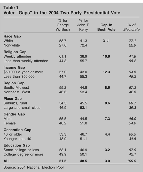
To set the stage for this exploration, it is useful to look at the relative size of key voting gaps in the closely contested 2004 presidential election. Table 1 presents evidence on eight voting gaps using the 2004 National Election Pool data (the national “exit poll” in 2004). Each “gap” is calculated as the net percentage difference in the vote for George W. Bush between the two categories. The gaps are listed in descending order of magnitude, with the overall two-party division at the bottom of the table (in bold) and the marginal distributions in the far right-hand column (in italics).
Voter “Gaps” in the 2004 Two-Party Presidential Vote

By far the largest of the voting gaps in 2004 was accounted for by race, or perhaps more accurately, race and ethnicity. George W. Bush obtained 58.7% of the White vote (which comprised 77.1% of the electorate), but just 27.6% of the non-White vote (22.9% of the electorate). Thus, the race gap was 31.1%, which is about 10 times larger than the overall Bush-Kerry vote differential overall (which was 3% in these data). Considering the difference between Whites and Blacks alone, the gap is nearly 48%, but the greater Republican vote among Latinos, Asians, and other non-Whites narrowed the gap.
The second largest gap in the 2004 presidential vote was the religion gap, or more precisely, the divide among those who do and do not worship at a church, synagogue, or mosque. At 16.8%, this gap was just a bit more than one-half the size of the race gap, and more than five times larger than the Bush-Kerry differential overall. Some two-thirds of those who reported attending worship weekly or more often voted for Bush, and nearly as many of the less-than-weekly attendees voted for John Kerry. Indeed, if the religion gap had been symmetrical and all else remained the same, Kerry would have obtained 52% of the popular vote—and quite possibly a lease on the White House. The religion gap is closely related to race, but in a complicated way: the weekly attendees include White evangelical Protestants, one of the strongest Republican constituencies, as well as Black Protestants, who are among the most loyal of Democrats. Indeed, the full range of religious variables, including both affiliation and attendance, produces very large gaps in the presidential vote. For example, the division between weekly attending White born-again Protestants and religiously unaffiliated voters was nearly 56 percentage points in 2004, rivaling the size of the gap between Whites and Blacks.
The class gap (which is really based on income) was the third most substantial voting gap in 2004. At 12.3%, it was about two-fifths the size of the race gap and a bit smaller than the religion gap—and roughly four times bigger than the Bush-Kerry vote difference overall. Voters with incomes of $50,000 a year or more voted 57% for Bush (about the same as Whites overall), while 55% of voters with an annual income below $50,000 voted for Kerry (about the same as less-than-weekly worship attendees). The income gap actually obscures the full range of the income variable: 64.1% of voters with incomes of $200,000 or more (3.4% of the total) voted for Bush, and 63.6% of those earning less than $15,000 (8.3% of the electorate) voted for Kerry. Voters with incomes between $30,000 and $50,000 broke almost evenly between the major party candidates.
The region and place gaps come next, each at 8.6%. These figures were almost three times the size of the overall Bush-Kerry vote differential. In a crude way, these geographic gaps represented the “red” and “blue” states—or to be more sophisticated, the “red” and “blue” localities within the states. Of course, creating dichotomous geographic measures is more than a bit arbitrary: Bush won the South quite handily, as well as a good bit of the Midwest, where there were many more close contests. Kerry won the Northeast and the West Coast, but lost the Mountain and Plains states, in some cases by small margins. Bush also won the suburbs, exurbs, and “no urbs” (rural areas). Meanwhile, Kerry won the urban vote, especially in the big cities. Presumably, places on the electoral map vary in the shade of red, blue, and purple in large part because of the kinds of people who live there.
At last we come to the gender gap, which ranked sixth out of the eight voting gaps at 7.3%. It is quite noteworthy that the gender gap was less than half the size of the religion gap in 2004. The major reason for this was Bush's success with women: he won nearly half of their votes. Meanwhile, Kerry failed to even up the score among men, losing that contest by a sizable 10 percentage points. Surely part of this story was a “marriage” gap: 58% of married voters backed Bush and 59% of the unmarried backed Kerry. Gender strengthens this relationship a bit, as 60% of married men voted to reelect the president while 62% of unmarried women voted to replace him.
The next-to-last gap in the 2004 presidential election was the generation gap. At only 4.4%, it was about a quarter the size of the religion gap and a third the size of the class gap. Voters over 40 years of age supported Bush on balance, while those under 40 were more likely to vote for Kerry. One reason for the small size of the generation gap is that age had a complex relationship with the 2004 vote. The very youngest voters (ages 18 to 24) went solidly for Kerry, but so did the very oldest voters (ages 75 and older). Bush did well with the middle-aged vote, but there was a good bit of variation, with his strongest support coming from 60- to 64-year olds. However, he nearly lost the 50- to 59-year-old vote.
The smallest of the voting gaps in 2004 was the education gap. At 3.2%, this gap was about one-tenth the size of the race gap. Bush won among those with less than a college degree, while the candidates broke even among those with college degrees and additional schooling. This dichotomy masks a strong curvilinear relationship. Kerry won the post-graduate vote by ten percentage points, and then just edged Bush out among voters without high school diplomas. In contrast, Bush won among high school, trade school, and college graduates with small majorities. Perhaps more than the other demographic factors discussed here, age and education are related to other gaps. Age and gender are linked to worship attendance; education to class and religious affiliation. And of course, age and education are closely related, given the increasing level of educational achievement of each successive generation.
A Peek at Multivariate Relationships
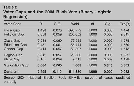
The possible links among these demographic factors begs the question of whether each has independent effects on the 2004 presidential vote. Although a full model of the vote is beyond the scope of this article, Table 2 offers a quick peek at this issue. These results are the product of binary logistic regression with the Bush vote coded “1” and the Kerry vote “0”; all the gaps are also coded dichotomously, with the category hypothesized to benefit Bush set as “1.”
Voter Gaps and the 2004 Bush Vote (Binary Logistic Regression)

The results are instructive. First, each and every one of the gaps, crude as they may be, is statistically significant in this multivariate analysis, with the exception of the generation gap. Second, the magnitude of the effects largely parallels the size of the gaps presented in Table 1, with the race, religion, and class gaps retaining their high rankings. Third, there are two important exceptions to the ordering of the gaps: the education and gender gaps now appear more important than they did in the original analysis. Here the education gap comes in just below the class gap in fourth place. This pattern is hardly surprising, since education is often conceptualized as a component of social class. The gender gap leapfrogs the geography gaps to fifth place, right behind education. These changes suggest that the electoral impact of region and place may in part reflect economic and cultural factors to which education and gender are central.
This crude analysis is designed to illuminate the popular and scholarly fascination with “gapology.” But certainly there is much more to be known about causes, consequences, and changes with regard to voting gaps, particularly as they affected the 2004 election and might be likely to affect the 2006 midterm elections. It is to a further exploration that we now turn in subsequent articles.
Biographies
Laura R. Olson is professor of political science at Clemson University. Recent books include (as co-author) Women with a Mission: Religion, Gender, and the Politics of Women Clergy (University of Alabama Press, 2005) and Religion and Politics in America: Faith, Culture, and Strategic Choices (Westview, 2003), and (as co-editor) Religious Interests in Community Conflict (Baylor University Press, forthcoming), The Encyclopedia of American Religion and Politics (Facts on File, 2003), and Christian Clergy in American Politics (Johns Hopkins University Press, 2001).
John C. Green is distinguished professor of political science and director of the Ray C. Bliss Institute of Applied Politics at the University of Akron. He is also a senior fellow with the Pew Forum on Religion and Public Life in Washington, D.C. He is co-author of The Bully Pulpit: The Politics of Protestant Clergy (University Press of Kansas, 1997); Religion and the Culture Wars: Dispatches From the Front (Rowman and Littlefield, 1996); and The Diminishing Divide: Religion's Changing Role in American Politics (Brookings Institution, 2000). In addition, he is co-editor of The State of the Parties (Rowman and Littlefield, 2003), now in its 5th edition, and Multiparty Politics in America (Rowman and Littlefield, 2002), in its 2nd edition.