1. Introduction
A small addition of long-chain polymers strongly affects the flow properties due to polymer stretching, which generates elastic stress and contributes to the nonlinear memory of the deformation history (Larson & Desai Reference Larson and Desai2015). These imparted rheological properties lead to various interesting flow phenomena, including elastic instabilities (Groisman & Steinberg Reference Groisman and Steinberg2000) in laminar flows and turbulent drag reduction (TDR) (Toms Reference Toms1949). Since drag reduction is linked to mass transport enhancement, an intriguing question arises about whether this also accompanies a similar variation in heat transport. Benzi, Ching & De Angelis (Reference Benzi, Ching and De Angelis2010) first conducted a direct numerical simulation (DNS) for homogeneous thermal convection in a box with periodic boundary conditions. It indicated that the addition of polymers can significantly enhance heat transport. However, the experiments by Ahlers & Nikolaenko (Reference Ahlers and Nikolaenko2010) on turbulent Rayleigh–Bénard convection (RBC) showed that polymer additives actually reduce heat transport, and this reduction increases with polymer concentration. They suggested that the results from Benzi et al. (Reference Benzi, Ching and De Angelis2010) are predominantly influenced by bulk flow, where all dissipation occurs in bulk and the boundary layer (BL) is absent, which is challenging to replicate experimentally. These studies indicate that heat transport is associated more with contributions from the boundary layer flow.
Understanding such a process is a continuous endeavour that has motivated more studies. Benzi, Ching & Chu (Reference Benzi, Ching and Chu2012) carried out a DNS study of a steady-state boundary layer flow involving polymers over a heated horizontal plate, using the Oldroyd-B model to describe the polymer solution (Bird et al. Reference Bird, Hassager, Armstrong and Curtis1987). Their findings revealed that the space-dependent effective viscosity induced by the polymers reduces the streamwise velocity near the plate. This scenario resulted in a reduction in heat transfer (HTR), with the extent of HTR increasing as polymer concentration rises, which agrees with the experimental observations of Ahlers & Nikolaenko (Reference Ahlers and Nikolaenko2010). In further research (Wei et al. Reference Wei, Ni and Xia2012, Reference Wei, Chen, Ni, Zhao and Xia2014), a series of experimental studies examined convection cells with either rough or smooth top and bottom plates. For cells with smooth plates, a reduction in heat transfer was documented, with a noticeable levelling off of this reduction as polymer concentration increased. Conversely, in the rough plate scenario, heat transfer enhancement (HTE) was observed under the same conditions, with an average increase of
 $4\,\%$
in the Nusselt number. A more detailed experimental analysis conducted in the rough cell indicated that the addition of a small quantity of polymers significantly enhances heat transport by suppressing incoherent heat fluxes and promoting coherent heat fluxes (Xie et al. Reference Xie, Huang, Funfschilling, Li, Ni and Xia2015). This provides direct experimental evidence of HTE due to the incorporation of polymers in the bulk region of turbulent thermal convection.
These experimental observations have inspired further theoretical studies. Benzi et al. (Reference Benzi, Ching, Yu and Wang2016) used the finitely extensible nonlinear elastic-Peterlin (FENE-P) model with a parameter
 $b^2$
to show that the transition from HTR to HTE could be written as a function of polymer concentration and relaxation time. The parameter
 $b^2$
represents the ratio between the maximum polymer length and the polymer length at equilibrium (Bird et al. Reference Bird, Hassager, Armstrong and Curtis1987). For cases with large
 $b^2$
, HTR increases with polymer concentration, which is consistent with their earlier study (Benzi et al. Reference Benzi, Ching and Chu2012) since the Oldroyd-B model is assumed as
 $b \rightarrow \infty$
in the FENE-P model. In contrast, heat transport was enhanced for cases with small
 $b^2$
. In their subsequent study (Benzi, Ching & De Angelis Reference Benzi, Ching and De Angelis2016), a non-monotonic behaviour of HTE was observed as the
 $Wi$
increased. This phenomenon was attributed to the competing influences of viscosity and polymer dynamics on the energy dissipation rate. Cheng et al. (Reference Cheng, Zhang, Cai, Li and Li2017) also reported a non-monotonic dependence of heat transport on
 $Wi$
, noting that heat transfer initially decreased with
 $Wi$
compared with that observed in Newtonian fluids, but began to increase beyond a critical
 $Wi$
value. Overall, their study indicated that heat transfer was reduced in polymer solutions when subjected to the same viscoelastic model. Therefore, there remains ongoing debate about whether adding polymer additives to a Newtonian solvent enhances or reduces heat transport. In a recent study, Dubief & Terrapon (Reference Dubief and Terrapon2020) continued to explore this topic, highlighting that the selection of HTE and HTR depends on both the maximum extensional viscosity and the relaxation time of the polymer solution.
The abovementioned numerical investigations, including recent studies by Wang et al. (Reference Wang, Ma, Cai, Zhang, Cheng and Zheng2020, Reference Wang, Cheng, Zhang, Zheng, Cai and Siginer2023), have primarily focused on several typical viscoelastic fluids, such as the Oldroyd-B and FENE-P models. These models are typically applicable to some unentangled polymer solutions and only include the polymer stretch relaxation time
 $\tau _R$
. For entangled polymer solutions or melts, an additional relaxation time is needed, known as the polymer orientation or disengagement time
 $\tau _d$
, to describe the properties relevant to flow. Furthermore, for strong flows, the extensibility parameter
 $\lambda _{max}$
is necessary to account for the finite extensibility of the polymer. The ratio
 $\tau _d / \tau _R$
depends on the degree of intermolecular entanglement of the polymer chains, which has a significant impact on their dynamic and rheological behaviours (Rothstein & Rothstein Reference Rothstein and McKinley2002; Larson & Desai Reference Larson and Desai2015). Consequently, it is then natural to ask whether the entanglement of polymers affects the heat transport in thermal convection.
Over the past three decades, understanding and modelling the nonlinear viscoelasticity of entangled polymer fluids has been a hot topic in many fields of science and engineering (Yang Reference Yang2002). Currently, the well-established tube model theory, which confines a polymer chain within a tube-like region, is widely regarded as the most effective method for describing the dynamics of entangled polymer melts (de Gennes Reference de Gennes1971; Doi & Edwards Reference Doi and Edwards1986). This theory posits that the main mechanism of stress relaxation in a linear regime is the chain’s ability to escape its original tube. However, the situation changes in nonlinear flows, where the convective constraint release (CCR) is considered the dominant mechanism of stress relaxation (Marrucci Reference Marrucci1996; Ianniruberto & Marrucci Reference Ianniruberto and Marrucci1996). In subsequent studies, more advanced models were proposed to account for the effects of CCR and stretching on the dynamics of entangled polymers (Mead, Larson & Doi Reference Mead, Larson and Doi1998; Milner, McLeish & Likhtman Reference Milner, McLeish and Likhtman2001; Graham et al. Reference Graham, Likhtman, McLeish and Milner2003). Among these models, the GLaMM model provides a microscopic description of CCR events and appropriately describes the interaction among CCR, chain stretching inside the tube and contour length fluctuations in monodisperse linear materials (Graham et al. Reference Graham, Likhtman, McLeish and Milner2003). This detailed modelling approach essentially requires a significant number of freedom degrees to depict the various tube segments of each chain, leading to substantial computational demands. Therefore, it is not suitable for numerical simulations in complex flow scenarios. The Rolie-Poly model addresses this limitation by simplifying the complete GLaMM model (Likhtman & Graham Reference Likhtman and Graham2003). It effectively describes linear entangled polymers with sufficient accuracy while maintaining computational simplicity. This constitutive model has primarily attracted widespread attention in simple flow scenarios, such as cross-slot flow (Liu et al. Reference Liu, Ouyang, Jiang, Zhuang and Li2016), homogeneous shear flow (Carter, Girkin & Fielding Reference Carter, Girkin and Fielding2016) and contraction flow (Liu et al. Reference Liu, Liu, Liu, Jiang and Ke2022). However, it has not yet been used in the study of thermal convection.
Similar to traditional RBC, natural convection heat transfer in a differentially heated cavity is also regarded as a canonical problem in thermal convection, which has garnered significant attention over the years (Ostrach Reference Ostrach1972; de Vahl Davis Reference de Vahl Davis1983; Le Quéré Reference Le Quéré1991; Fusegi & Hyun Reference Fusegi and Hyun1994). Most early studies on this benchmark problem were conducted in Newtonian fluids (Dixit & Babu Reference Dixit and Babu2006; Xu, Shi & Zhao Reference Xu, Shi and Zhao2017; Polasanapalli & Anupindi Reference Polasanapalli and Anupindi2019; Xu, Shi & Xi Reference Xu, Shi and Xi2019) or non-Newtonian visco-inelastic fluids (Turan et al. Reference Turan, Chakraborty and Poole2010, Reference Turan, Sachdeva, Chakraborty and Poole2011, Reference Turan, Sachdeva, Poole and Chakraborty2012, 2013) to investigate flow states, heat transport and bifurcation. In classic RBC, the formation of convective motion has a threshold beyond which the thermal heterogeneity induced by buoyancy overcomes stability effects, such as viscosity. This phenomenon can be described as an exchange of stability occurring at the critical Rayleigh number, where the stability of the quiescent state is exchanged with that of the convective state (Bergé & Dubois Reference Bergé and Dubois1984). Once convective motion begins, denser fluid elements descend while less dense fluid elements ascend with equal probability due to symmetry. As a result, the onset of RBC experiences a bifurcation with two symmetrical branches because of this equiprobability. However, this ambiguity in the direction of motion does not occur in natural convection within a differentially heated cavity. In this set-up, there is a natural upward movement at the hot plate and a downward movement at the cold plate due to horizontal temperature gradients. Unlike RBC, there is no threshold for this thermal convection and the flow is more stable. Paolucci & Chenoweth (Reference Paolucci and Chenoweth1989) conducted a numerical investigation into the transition from laminar to chaotic flow in a differentially heated square cavity. The flow regimes they explored included steady-state, periodic oscillation, quasi-periodic flow and chaotic flow. These were illustrated through time histories, spectral analysis and streamlines at various time intervals. Henkes & Hoogendoorn (Reference Henkes and Hoogendoorn1990) studied the stability of natural convection for water within a similar cavity. Their numerical results indicated that the flow converges to a steady state in an oscillatory manner when the critical Rayleigh number is approximately
 $Ra_{cr} \sim 4 \times 10^9$
, in agreement with the experimental observations by Ivey (Reference Ivey1984). They suggested that the flow instability relates to both Rayleigh/Bénard and Tollmien–Schlichting instabilities, a proposition later confirmed by a recent experimental study conducted by Kishor, Singh & Srivastava (Reference Kishor, Singh and Srivastava2020). Le Quéré & Behnia (Reference Le Quéré and Behnia1998) carried out a DNS investigation on two-dimensional natural convection in air-filled differentially heated cavities with adiabatic horizontal walls. Their study revealed the onset of unsteadiness, the route to chaos and the dynamics of fully chaotic natural convection. In subsequent research, they revisited this issue using stability analysis algorithms and provided accurate Hopf bifurcation points for several unstable modes in cavities with aspect ratios ranging from
 $1$
to
 $7$
(Xin & Le Quéré Reference Xin and Le Quéré2006). Zhao & Tian (Reference Zhao and Tian2016) numerically examined the natural convection flows in a square cavity using a higher-order accuracy numerical method, which agreed well with the results obtained by Le Quéré & Behnia (Reference Le Quéré and Behnia1998). Their findings indicated that the flow first loses stability through a Hopf bifurcation at
 $Ra_{c1}$
to a periodic flow, then undergoes a second bifurcation into a quasi-periodic flow at
 $Ra_{c2}$
and ultimately evolves into turbulence through further bifurcations.
These abovementioned studies are limited to Newtonian fluids. Chauhan, Sahu & Sasmal (Reference Chauhan, Sahu and Sasmal2021) first investigated two-dimensional natural convection in a differentially heated square cavity filled with unentangled solutions, modelled using the FENE-P constitutive model. They found that heat transfer is reduced as the polymer viscosity ratio and polymer extensibility parameter increases. However, for more concentrated solutions or melts, the impact of entangled polymers on heat transfer and bifurcation in natural convection remains unclear, particularly in scenarios involving strong elasticity. In this paper, we follow Chauhan et al. (Reference Chauhan, Sahu and Sasmal2021) and aim to examine the dependence of heat transfer and bifurcation of natural convection on control parameters in entangled polymer solutions or melts. The entangled polymers are modelled by the Rolie-Poly framework, which incorporates a nonlinear spring coefficient (Kabanemi & Hétu Reference Kabanemi and Hétu2009). We carry out numerical simulations with a fixed Prandtl number (
 $Pr = 7$
) and a broad range of Rayleigh numbers (
 $10^3\leqslant Ra \leqslant 10^{9}$
). By restricting our study to two spatial dimensions, we avoid potentially significant three-dimensional nonlinear effects that can arise from vortex stretching (Paolucci & Chenoweth Reference Paolucci and Chenoweth1989). Given our limitations in computational resources, this approach is more cost-effective and manageable for our parametric study. To better identify and visualise the effect of polymers, we focus primarily on flow states at low Rayleigh numbers, while also examining heat transfer at higher Rayleigh numbers. These heat performances are analysed in conjunction with boundary layer dynamics and the kinetic energy budget. In addition, we observe bifurcation phenomena at low Rayleigh numbers as the polymer elasticity increases. Then, the bifurcation routes driven by inertia and elasticity are examined in numerical experiments. These results are presented by time histories, Fourier spectra analysis and spatial structures observed at varying time intervals.
The remainder of the present paper is organised as follows. In § 2, we describe the physical problem and the numerical method employed. Section 3 presents the rheological analysis based on the Rolie-Poly model. In § 4, we discuss the results obtained, including the spatial structure of the flow under weak and strong elasticity, the dependence of heat transport on various parameters, and bifurcation phenomena. Finally, we summarise our findings in § 5.
Sketch of the present problem.

2. Numerical model
2.1. Governing equations
In this study, we consider the two-dimensional natural convection in a square cavity of length
 $H$
filled with the linear entangled polymer solution, as shown in figure 1. The temperature difference between the left and right walls is
 $\Delta {T}=T_1-T_0$
and adiabatic boundary conditions are set at the top and bottom walls. The non-slip boundary conditions are considered for the velocity at all solid walls of the cavity. With the Oberbeck–Boussinesq approximation, the physical problem is described by the following form of equations for the conservation of mass, momentum and energy:
 \begin{align} \nabla \cdot \boldsymbol{u} = 0, \end{align}
 \begin{align} \frac {\partial \boldsymbol{u}}{\partial t} + (\boldsymbol{u} \cdot \nabla ) \boldsymbol{u} = -\frac {1}{\rho } \nabla {p} + \frac {1}{\rho } \nabla \cdot \boldsymbol{\tau } + \alpha g (T - T_{0}) \boldsymbol{e}_y, \end{align}
 \begin{align} \frac {\partial T}{\partial t} + (\boldsymbol{u} \cdot \nabla ) T = \kappa {\nabla }^2 T. \end{align}
Within the classical Oberbeck–Boussinesq approximation, the thermo-physical properties of the polymer solution, e.g. the thermal expansion coefficient
 $\alpha$
, thermal diffusivity
 $\kappa$
, density
 $\rho$
and gravity acceleration
 $g$
, are treated as independent of the temperature, except that the density of the buoyancy term in the momentum equation is assumed to be linearly correlated with the temperature. In the abovementioned equations,
 $\boldsymbol{u} = [u,v ]$
is the velocity field,
 $t$
is the time,
 $p$
is the pressure,
 $T$
is the temperature and
 $\boldsymbol{e}_y$
denotes the unit vector in the vertical direction. Here,
 $\boldsymbol{\tau }$
is the total extra stress tensor, which consists of the Newtonian solvent (
 $\boldsymbol{\tau }_s$
) and polymer (
 $\boldsymbol{\tau }_p$
) stress tensors as follows:
 \begin{align} \boldsymbol{\tau } = \boldsymbol{\tau }_s + \boldsymbol{\tau }_p. \end{align}
In (2.4),
 $\boldsymbol{\tau }_s$
is given by
 $\boldsymbol{\tau }_s = \eta _s (\nabla \boldsymbol{u} + \nabla {\boldsymbol{u}}^T)$
, where
 $\eta _s$
is the solvent viscosity,
 $\nabla \boldsymbol{u}$
is the velocity gradient tensor and
 ${\nabla \boldsymbol{u}}^T$
denotes the transposition of the velocity gradient tensor.
In the studies for describing the microscopic theory of entangled polymer chains, Graham et al. (Reference Graham, Likhtman, McLeish and Milner2003) proposed an improved version of the tube model (Doi & Edwards Reference Doi and Edwards1986) which can describe the processes of the repetition, CCR, constraint release driven by repetition, chain stretching and contour length fluctuations (CLFs). In their subsequent study, Likhtman & Graham (Reference Likhtman and Graham2003) derived a simplified constitutive equation from the complete theory, named the Rolie-Poly constitutive equation. This model can capture the rheological response of entangled polymers, such as the monodisperse polystyrene solution (Ye et al. Reference Ye, Larson, Pattamaprom and Sridhar2003). In this study, the Rolie-Poly model is used to describe the stress–strain relationship of the linearly entangled polymer solution, which is written in the form as follows:
 \begin{align} \tau _d \left [\frac {\partial \boldsymbol{\sigma }}{\partial t} + (\boldsymbol{u} \cdot \nabla ) \boldsymbol{\sigma } - (\nabla \boldsymbol{u} \cdot \boldsymbol{\sigma } + \boldsymbol{\sigma } \cdot \nabla {\boldsymbol{u}}^T)\right ] = - (\boldsymbol{\sigma } - \boldsymbol{I}) \nonumber \\[8pt] - 2 \xi \left [1-\sqrt {\frac {3}{\textrm {tr} (\boldsymbol{\sigma })}}\right ] \left (\boldsymbol{\sigma } + \beta _{R} \left [\frac {\textrm {tr} (\boldsymbol{\sigma })}{3}\right ]^\delta (\boldsymbol{\sigma }-\boldsymbol{I})\right ), \end{align}
where
 $\boldsymbol{\sigma }$
is the conformation tensor of the polymer and
 $\textrm {tr} (\boldsymbol{\sigma })$
represents the trace of a tensor. Here,
 $\xi$
is defined as the ratio of the reptation time
 $\tau _d$
to the Rouse relaxation time or stretch time
 $\tau _R$
, i.e.
 $\xi = {\tau _d}/{\tau _R}$
(we call it the relaxation time ratio here), which describes the degree of entanglement in polymer chains (Reis & Wilson Reference Reis and Wilson2013; Larson & Desai Reference Larson and Desai2015; Keithley et al. Reference Keithley, Palmerio, Escobedo, Bartlett, Huang, Villasmil and Cromer2023). For highly entangled polymer chains, its reptation occurs much more slowly than the relaxation caused by chain stretch (Hoyle & Fielding Reference Hoyle and Fielding2017), which means that orientation relaxation becomes the main mechanism for stress relaxation. Additionally,
 $\beta _{R}$
is the CCR coefficient similar to the coefficient which is introduced by Marrucci (Reference Marrucci1996),
 $\delta$
is a negative power fitted by the full theory (Graham et al. Reference Graham, Likhtman, McLeish and Milner2003), which is taken to be
 $-0.5$
in the current work,
 $\boldsymbol{I}$
is the identity matrix and
 $\boldsymbol{\sigma } = \boldsymbol{I}$
denotes the equilibrium value of the conformational tensor without flow (Likhtman & Graham Reference Likhtman and Graham2003).
However, the original Rolie-Poly model does not consider finite extensibility, which tends to restrict the degree of strain hardening for polymer chains in the stretching regime (Graham et al. Reference Graham, Likhtman, McLeish and Milner2003; Likhtman & Graham Reference Likhtman and Graham2003). Kabanemi & Hétu (Reference Kabanemi and Hétu2009) considered the non-Gaussian behaviour of polymer chains in fast flows and introduced a nonlinear spring coefficient to emphasise the finite extensibility of polymer chains, which is defined as
 \begin{align} k_s(\lambda ) = \frac {\big(3 - {\lambda }^2 / {\lambda _{max}^2}\big) \big(1 - 1 / {\lambda _{max}^2}\big)}{\big(1 - {\lambda }^2 / {\lambda _{max}^2}\big) \big(3 - 1 / {\lambda _{max}^2}\big)}, \end{align}
where
 $\lambda = {l}/{l_0} = \sqrt {{\textrm {tr} (\boldsymbol{\sigma })}/{3}}$
is the ratio of the chain stretch and
 $\lambda _{max}$
is the fixed maximum stretch ratio. The length
 $l$
denotes the current length of the tube occupied by an entangled segment, where
 $l_0$
is the length of the same tube segment in the equilibrium state. Therefore, the non-Gaussian version of the Rolie-Poly model is written in the following form (Kabanemi & Hétu Reference Kabanemi and Hétu2009):
 \begin{align} \tau _d \left [\frac {\partial \boldsymbol{\sigma }}{\partial t} + (\boldsymbol{u} \cdot \nabla ) \boldsymbol{\sigma } - (\nabla \boldsymbol{u} \cdot \boldsymbol{\sigma } + \boldsymbol{\sigma } \cdot \nabla {\boldsymbol{u}}^T)\right ] = - (\boldsymbol{\sigma } - \boldsymbol{I}) \nonumber \\[8pt] - 2 \xi k_s(\lambda ) \left [1-\sqrt {\frac {3}{\textrm {tr} (\boldsymbol{\sigma })}}\right ] \left (\boldsymbol{\sigma } + \beta _{R} \left [\frac {\textrm {tr} (\boldsymbol{\sigma })}{3}\right ]^\delta (\boldsymbol{\sigma }-\boldsymbol{I})\right ). \end{align}
The relationship between the stress tensor and conformation tensor is defined as
 \begin{align} \boldsymbol{\tau }_p = \frac {\eta _p}{\tau _d} k_s(\lambda ) (\boldsymbol{\sigma } - \boldsymbol{I}), \end{align}
where
 $\eta _p$
is the polymer viscosity which denotes the contribution from the polymer.
The above-governing equation can be written in dimensionless form by the following transformations:
 \begin{align} \boldsymbol{x}^\ast = \frac {\boldsymbol{x}}{H}, \quad \boldsymbol{u}^\ast = \frac {\boldsymbol{u}}{u_c}, \quad t^\ast = \frac {t}{H / u_c}, \quad p^\ast = \frac {p}{\rho u_c^2}, \quad \theta ^\ast = \frac {T-T_0}{T_1-T_0}, \end{align}
where
 $u_c = \sqrt {\alpha g H \Delta T}$
is the characteristic velocity scale. For convenience, the asterisk has been omitted in the subsequent dimensionless governing equation as follows:
 \begin{align} \nabla \cdot \boldsymbol{u} = 0, \end{align}
 \begin{align} \frac {\partial \boldsymbol{u}}{\partial t} + (\boldsymbol{u} \cdot \nabla ) \boldsymbol{u} = -\nabla {p} + \frac {\beta }{\sqrt {Ra/Pr}} {\nabla }^2 \boldsymbol{u} + \frac {(1 - \beta )}{Wi \sqrt {Ra/Pr}} \nabla \cdot \left [k_s(\lambda ) (\boldsymbol{\sigma } - \boldsymbol{I})\right ] + \theta \boldsymbol{e}_y, \end{align}
 \begin{align} \frac {\partial \theta }{\partial t} + (\boldsymbol{u} \cdot \nabla ) \theta = \frac {1}{\sqrt {Ra Pr}} {\nabla }^2 \theta , \end{align}
 \begin{align} Wi \left [\frac {\partial \boldsymbol{\sigma }}{\partial t} + (\boldsymbol{u} \cdot \nabla ) \boldsymbol{\sigma } - (\nabla \boldsymbol{u} \cdot \boldsymbol{\sigma } + \boldsymbol{\sigma } \cdot \nabla {\boldsymbol{u}}^T)\right ] = - (\boldsymbol{\sigma } - \boldsymbol{I}) \nonumber \\[8pt] - 2 \xi k_s(\lambda ) \left [1-\sqrt {\frac {3}{\textrm {tr} (\boldsymbol{\sigma })}}\right ] \left (\boldsymbol{\sigma } + \beta _{R} \left [\frac {\textrm {tr} (\boldsymbol{\sigma })}{3}\right ]^\delta (\boldsymbol{\sigma }-\boldsymbol{I})\right ). \end{align}
In the abovementioned non-dimensional equations, several dimensionless parameters governing the coupling process of flow and heat transfer can be defined as follows:
 \begin{align} Pr = \frac {\upsilon }{\kappa }, \quad Ra = \frac {\alpha g \Delta T H^3}{\upsilon \kappa }, \quad Wi = \frac {\tau _d u_c}{H}, \quad \beta = \frac {\eta _s}{\eta _0}, \end{align}
where
 $Pr$
is the Prandtl number, which represents the ratio of the momentum to the thermal diffusion. The Rayleigh number (
 $Ra$
) denotes the ratio of the buoyancy force to the viscous force, where
 $\upsilon = {\eta _0}/{\rho }$
is the kinematic viscosity. The Weissenberg number (
 $Wi$
) is defined as the ratio between the longest relaxation time of the entangled polymer solution and the characteristic time of the flow. Lastly,
 $\beta$
is the viscosity ratio, which represents the ratio of the solvent viscosity
 $\eta _s$
to the total viscosity
 $\eta _0 = \eta _s + \eta _p$
at zero-shear rate. In addition to these dimensionless numbers, the relaxation time ratio
 $\xi$
, the CCR coefficient
 $\beta _{R}$
and the fixed maximum stretch ratio
 $\lambda _{max}$
are also the model parameters considered in this study.
In the current study, the local and global transport properties of heat transfer are quantified by local Nusselt numbers and corresponding average Nusselt numbers respectively
 \begin{align} Nu_l = \frac {h_l H}{k} = -\frac {\partial \theta }{\partial x}\mid _{x=0},\quad Nu = \frac {h H}{k} = \frac {1}{y}\int _{0}^{y} Nu_l\, \textrm {d}y, \end{align}
where
 $h_l$
and
 $h$
are the coefficient of local and average heat transfer, respectively.
Finally, the no-slip boundary conditions, i.e.
 $\boldsymbol{u}=0$
, are applied at all walls for the velocity. For the temperature field, the adiabatic conditions are imposed at the top and bottom walls,
 ${\partial \theta }/{\partial \boldsymbol{n}} = 0$
, where
 $\boldsymbol{n}$
denotes the direction normal to the wall. The fixed temperatures
 $\theta _1 = 1$
and
 $\theta _0 = 0$
are set at the left and right walls, respectively. In addition,
 $\boldsymbol{\sigma }$
is linearly extrapolated at all solid walls with second-order accuracy (Pimenta & Alves Reference Pimenta and Alves2017; Alves, Oliveira & Pinho Reference Alves, Oliveira and Pinho2021).
2.2. The log-conformation reformulation
For viscoelastic fluids, the stress of the polymer grows exponentially at moderately large values of the Weissenberg number, which results in severe numerical divergence in simulation (Keunings Reference Keunings1986). Therefore, the log-conformation reformulation (LCR) (Fattal & Kupferman Reference Fattal and Kupferman2005; Zhang et al. Reference Zhang, Li, Wang, Ma, Zhang, Yu and Li2021) is adopted to ensure the numerical stability in this work.
In the LCR method, the conformation tensor
 $\boldsymbol{\sigma }$
is diagonalised,
 $\boldsymbol{\sigma } = \boldsymbol{R} \boldsymbol{\Lambda } \boldsymbol{R}^T$
, where the diagonal matrix
 $\boldsymbol{\Lambda }$
and the orthogonal matrix
 $\boldsymbol{R}$
are composed of its eigenvalues and eigenvectors, respectively (Fattal & Kupferman Reference Fattal and Kupferman2005). Then, the velocity gradient tensor
 $\nabla \boldsymbol{u}$
is decomposed as
 \begin{align} \nabla \boldsymbol{u} = \boldsymbol{\Omega } + \boldsymbol{B} + \boldsymbol{N} \boldsymbol{\sigma }^{-1}, \end{align}
where
 $\boldsymbol{\Omega }$
and
 $\boldsymbol{N}$
are antisymmetric tensors and
 $\boldsymbol{B}$
is the symmetric tensor, which is defined by Fattal & Kupferman (Reference Fattal and Kupferman2005). So here is not to repeat. Substituting of (2.16) into (2.13) yields
 \begin{align} Wi \left [\frac {\partial \boldsymbol{\sigma }}{\partial t} + (\boldsymbol{u} \cdot \nabla ) \boldsymbol{\sigma } - (\boldsymbol{\Omega } \cdot \boldsymbol{\sigma } - \boldsymbol{\sigma } \cdot \boldsymbol{\Omega }) - 2 \boldsymbol{B} \cdot \boldsymbol{\sigma }\right ] = - (\boldsymbol{\sigma } - \boldsymbol{I}) \nonumber \\[8pt] - 2 \xi k_s(\lambda ) \left [1-\sqrt {\frac {3}{\textrm {tr} (\boldsymbol{\sigma })}}\right ] \left (\boldsymbol{\sigma } + \beta _{R} \left [\frac {\textrm {tr} (\boldsymbol{\sigma })}{3}\right ]^\delta (\boldsymbol{\sigma }-\boldsymbol{I})\right ). \end{align}
A new tensor
 $\boldsymbol{\psi }$
is defined as the natural logarithm of
 $\boldsymbol{\sigma }$
,
 \begin{align} \boldsymbol{\psi } = \ln (\boldsymbol{\sigma }) = \boldsymbol{R} \ln (\boldsymbol{\Lambda }) \boldsymbol{R}^T. \end{align}
Equation (2.17) can be decomposed into its four constituents, namely, the advection term, rotation term, extension term and source term, which are mapped into the logarithmic domain (Fattal & Kupferman Reference Fattal and Kupferman2005). These four constituents can be added up since the time derivative of
 $\boldsymbol{\psi }$
is a linear transformation of the time derivative of
 $\boldsymbol{\sigma }$
(Kenney & Laub Reference Kenney and Laub1998), which derives the constitutive equation for the log-conformation tensor as follows:
 \begin{align} Wi \left [\frac {\partial \boldsymbol{\psi }}{\partial t} + (\boldsymbol{u} \cdot \nabla ) \boldsymbol{\psi } - (\boldsymbol{\Omega } \cdot \boldsymbol{\psi } - \boldsymbol{\psi } \cdot \boldsymbol{\Omega }) - 2 \boldsymbol{B}\right ] = - e^{-\boldsymbol{\psi }} \left ((e^{\boldsymbol{\psi }} - \boldsymbol{I})\vphantom{\left [\frac {{\textrm {tr}} (e^{\boldsymbol{\psi }})}{3}\right ]^\delta}\right . \nonumber \\\left .- 2 \xi k_s(\lambda ) \left [1-\sqrt {\frac {3}{{\textrm {tr}} (e^{\boldsymbol{\psi }})}}\right ] \left (e^{\boldsymbol{\psi }} + \beta _{R} \left [\frac {{\textrm {tr}} (e^{\boldsymbol{\psi }})}{3}\right ]^\delta (e^{\boldsymbol{\psi }} - \boldsymbol{I})\right ) \right ). \end{align}
2.3. Discretisation and numerical method
The constitutive equation coupled with other governing equations, i.e. the mass, momentum and energy equations, have been solved by the open-source CFD platform OpenFOAM
 $^{\circledR }$
with the rheotool toolbox (Pimenta & Alves Reference Pimenta and Alves2017). In the present study, the gradient and divergence terms in all governing equations are discretised by the Gauss linear interpolation scheme, while the terms related to the time derivative are discretised by the Euler scheme. The second-order accurate Gauss linear orthogonal interpolation scheme is considered for the diffusion terms in both the momentum and energy equations. The advection terms are discretised by the high-resolution convergent and universally bounded interpolation scheme for the treatment of advection (CUBISTA) to improve iteration convergence (Alves, Oliveira & Pinho Reference Alves, Oliveira and Pinho2003).
For the selection of solvers, the velocity field, temperature field and stress field are solved by the preconditioned biconjugate gradient solver (PBiCG) with diagonal-based incomplete LU (DILU) preconditioner (Lee, Zhang & Lu Reference Lee, Zhang and Lu2003), where the relative tolerance level is set to
 $10^{-8}$
. Next, the pressure field is solved by the preconditioned conjugate (PCG) solver with the diagonal-based incomplete Cholesky (DIC) preconditioner (Chauhan et al. Reference Chauhan, Sahu and Sasmal2021), where the relative tolerance level is set to
 $10^{-10}$
. The decoupling of velocity and pressure is considered for using the SIMPLE method. Furthermore, the stress–velocity coupling method proposed by Pimenta & Alves (Reference Pimenta and Alves2017) is used to avoid the decoupling problems.
The correctness and accuracy of the code are verified from two aspects: the natural convection of Newtonian fluids in a differentially heated cavity and the constitutive model of entangled polymers. We first present the distributions of non-dimensional temperature along the horizontal mid-plane of the differentially heated cavity filled with air
 $(Pr = 0.71)$
for a range of
 $Ra$
in figure 2, in agreement with the results of Chauhan et al. (Reference Chauhan, Sahu and Sasmal2021). Table 1 shows a comparison between the current results and those from the corresponding literature. Overall, all the results demonstrate excellent agreement.
Comparison of non-dimensional temperature profiles along the horizontal mid-plane of the cavity with Chauhan et al. (Reference Chauhan, Sahu and Sasmal2021) at
 $Pr = 0.71$
.

However, the validation of our constitutive model is conducted using numerical results from the uniaxial extensional flow of the entangled polymer solution, which is described by the Rolie-Poly model. The following constitutive parameters are considered in our constitutive model:
 $\eta _0 = 3.9 \times 10^4 \ \textrm {Pa} \cdot \textrm{s}$
,
 $\beta = 0.9$
,
 $\tau _d = 192.7 \ \textrm {s}$
,
 $\tau _R = 5 \ \textrm {s}$
,
 $\beta _R = 0.1$
and
 $\delta = -0.5$
, where
 $\lambda _{max}$
is set to
 $6$
and
 $8$
, respectively (Kabanemi & Hétu Reference Kabanemi and Hétu2009). As shown in figure 3, our present results are greatly consistent with the prediction available in the literature for different
 $\lambda _{max}$
.
Comparison between the present results and the literature results at
 $Pr = 0.71$
.

Steady-state extensional stress for the uniaxial extensional flow compared with the prediction of Kabanemi & Hétu (Reference Kabanemi and Hétu2009).

To effectively balance computational cost and accuracy in our numerical investigations, we systematically validate grid independence at
 $Ra = 10^6$
and
 $Ra = 10^9$
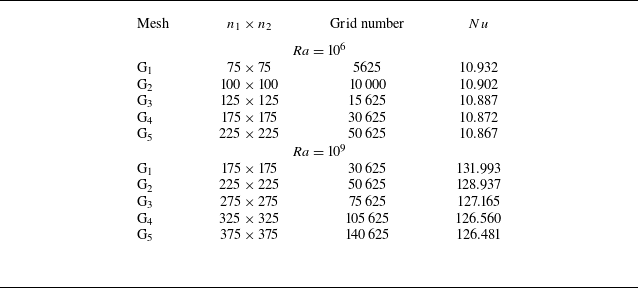
. A series of grids with different numbers of hexahedral cells are generated for the whole computational domain. The dense grids are concentrated near the solid walls of the square cavity to better capture the behaviour of polymer stress and velocity in these regions (Chauhan et al. Reference Chauhan, Sahu and Sasmal2021). Table 2 shows the average Nusselt numbers for different grid densities, where
 $n_1$
and
 $n_2$
represent the number of grids in the
 $x$
and
 $y$
directions, respectively. As the grid number
 $n$
increases,
 $Nu$
gradually decreases and tends to stabilise. At
 $Ra = 10^6$
, the difference of
 $Nu$
is less than
 $0.05\,\%$
when
 $n$
reaches
 $175$
. The grid
 $\textrm {G}_4$
(
 $n_1 \times n_2 = 75 \times 75$
) with a court of
 $30\,625$
cells is entirely sufficient for the numerical simulations at low
 $Ra$
. At
 $Ra = 10^9$
,
 $Nu$
tends to stabilise at higher grid densities, where the difference of
 $Nu$
between
 $\textrm {G}_4$
(
 $n_1 \times n_2 = 325 \times 325$
) and
 $\textrm {G}_5$
(
 $n_1 \times n_2 = 375 \times 375$
) is approximately
 $0.06\,\%$
. Therefore, the grid
 $\textrm {G}_4$
(
 $n_1 \times n_2 = 325 \times 325$
) is used for the numerical simulations at high
 $Ra$
.
Comparison of
 $Nu$
with different grid densities at
 $Ra = 10^6$
and
 $Ra = 10^9$
. The other parameters are
 $Pr = 7$
,
 $Wi = 10$
,
 $\beta = 0.5$
,
 $\xi = 1$
,
 $\lambda _{max} = 10$
and
 $\beta _R$
= 0.5.

3. Rheology of the Rolie-Poly model
Before embarking on the discussion of our results, we hope to first analyse the rheological properties of the Rolie-Poly model in steady-state shear and planar extensional flow, which can help us understand the numerical results given in § 4 and connect the flow structure and heat transport with the microstructure of a linear entangled polymer.
Previous studies have demonstrated that the Rolie-Poly model can predict significant shear-thinning characteristics (Reis & Wilson Reference Reis and Wilson2013), which is similar to the Giesekus (Peng et al. Reference Peng, Li, Xiong, Xu and Yu2021) and FENE-P models (Keithley et al. Reference Keithley, Palmerio, Escobedo, Bartlett, Huang, Villasmil and Cromer2023). We simulated the rheological properties of the Rolie-Poly model at
 $\beta = 0.1$
with different model parameters, including the relaxation-time ratio (
 $0.2 \leqslant \xi \leqslant 5$
), the CCR parameter (
 $0.1 \leqslant \beta _R \leqslant 0.9$
) and fixed maximum stretch ratio (
 $4 \leqslant \lambda _{max} \leqslant 10$
). The selection of
 $\xi$
,
 $\beta _R$
and
 $\lambda _{max}$
is based on the rheological response of the actual linear entangled polymer solution (Ye et al. Reference Ye, Larson, Pattamaprom and Sridhar2003; Kabanemi & Hétu Reference Kabanemi and Hétu2009; Liu et al. Reference Liu, Ouyang, Jiang, Zhuang and Li2016).
The first and second normal stress differences are expressed as
 \begin{align} N_1 = \tau _{xx} - \tau _{yy}, \quad N_2 = \tau _{yy} - \tau _{zz}. \end{align}
The normal-stress-difference coefficients in steady-state shear flow can be defined as
 \begin{align} \Psi _{1} = \frac {N_1}{\eta _p \dot {\gamma }},\quad \Psi _{2} = \frac {N_2}{\eta _p \dot {\gamma }}, \end{align}
where
 $\dot {\gamma }$
is the steady-state shear strain rate. The normal-stress-difference coefficients in planar extensional flow are defined as
 \begin{align} \Psi _{1} = \frac {N_1}{\eta _p \dot {\varepsilon }},\quad \Psi _{2} = \frac {N_2}{\eta _p \dot {\varepsilon }}, \end{align}
where
 $\dot {\varepsilon }$
is the steady-state planar extensional strain rate.
(a) Steady shear viscosity, (b) first normal-stress-difference coefficient, (c) steady planar extensional viscosity and (d) first normal stress difference of the Rolie-Poly model at
 $\beta = 0.1$
.

The steady shear viscosity of the Rolie-Poly model with different model parameters is shown in figure 4(a), where the steady shear viscosity is written in the normalised form as
 $\eta /\eta _0$
. Here,
 $\eta /\eta _0$
decreases with
 $Wi = \tau _d \dot {\gamma }$
for all constitutive model parameters except for
 $\xi = 0.2$
, which exhibits typical shear-thinning characteristics, and the degree of shear-thinning gradually decreases with the decrease value of
 $\xi$
. However, the monotonicity is lost at large shear rates and the steady shear viscosity presents a brief trend of shear-thickening for
 $\xi = 0.2$
, which indicates that the Rolie-Poly model can predict non-monotonic behaviour by adjusting the model parameters (Reis & Wilson Reference Reis and Wilson2013). In a recent study (Keithley et al. Reference Keithley, Palmerio, Escobedo, Bartlett, Huang, Villasmil and Cromer2023), the Rolie-Poly model consistently exhibits noticeable shear-thinning characteristics at high
 $\xi$
(
 $\xi \geqslant 30$
). Therefore, it demonstrates that when orientation relaxation becomes the main mechanism of stress relaxation (
 $\tau _d$
is greater than
 $\tau _R$
), the Rolie-Poly model can predict shear-thinning. However, the Rolie-Poly model tends to exhibit shear-thickening characteristics when the stretch relaxation becomes the main mechanism of stress relaxation (
 $\tau _d$
is less than
 $\tau _R$
). It is important to note that the effect of
 $\beta _R$
and
 $\lambda _{max}$
on the steady shear viscosity is not significant.
The normal stress difference is the main manifestation of elasticity in polymer materials. As illustrated in figure 4(b), the first normal-stress-difference coefficient
 $\Psi _1$
is consistently positive and monotonically increases with the steady-state shear rate across all model parameters, except when
 $\xi = 5$
. In this particular case,
 $\Psi _1$
displays a notable non-monotonic trend: it initially increases, then gradually decreases and finally shows a slight increase again. Additionally,
 $\Psi _1$
decreases as
 $\lambda _{max}$
reduces at high shear rates, indicating that
 $\lambda _{max}$
is significant only in scenarios involving strong elasticity. The second normal stress difference is zero because
 $\tau _{yy}$
equals
 $\tau _{zz}$
in both simple shear and planar extensional flow.
The steady planar extensional viscosity of the Rolie-Poly model for
 $\beta = 0.1$
is shown in figure 4(c), where the steady planar extensional viscosity can be expressed in the normalised form as
 $\eta _E / 3\eta _p$
due to
 $\eta _E = 3\eta _p$
in a Newtonian fluid. Here,
 $\eta _E / 3\eta _p$
first increases rapidly with
 $Wi = \tau _d \dot {\varepsilon }$
and then it reaches a constant value. A higher extensional viscosity tends to appear at lower
 $\xi$
. However, for
 $\xi = 5$
, after the initial stable period,
 $\eta _E / 3\eta _p$
first decreases with
 $Wi$
before rapidly increasing again, eventually approaching a stable value. In the appendix material of Keithley et al. (Reference Keithley, Palmerio, Escobedo, Bartlett, Huang, Villasmil and Cromer2023), the Rolie-Poly model also predicts thinning followed by thickening at high
 $\xi$
(
 $\xi \geqslant 30$
). The thickening often occurs at
 $\dot {\varepsilon } = \xi$
(Keithley et al. Reference Keithley, Palmerio, Escobedo, Bartlett, Huang, Villasmil and Cromer2023), which is consistent with our results at
 $\xi = 5$
. In particular, it is different from the simple shear flow that
 $\lambda _{max}$
begins to affect the steady planar extensional viscosity at lower
 $Wi$
(
 $Wi \approx 1$
), which decreases with the decreasing value of
 $\lambda _{max}$
.
Figure 4(d) shows that the first normal stress difference
 $N_1$
monotonically increases with
 $Wi$
for all the model parameters. The increase of
 $\xi$
causes a delay in the onset of rapid growth of
 $N_1$
. In general, whether it is a simple shear flow or planar extensional flow, the effect of
 $\beta _R$
on the rheological properties of the Rolie-Poly model is small. Based on our preliminary work, we discovered that minor variations in rheological properties have little effect on flow structure and heat transport. Therefore, we have decided to fix
 $\beta _R$
at
 $0.5$
and exclude its impact from our subsequent discussion.
4. Results and discussion
This section presents a comprehensive numerical investigation of various conditions, including the following parameters: Rayleigh number (
 $10^3\leqslant Ra \leqslant 10^{9}$
), Weissenberg number (
 $1 \leqslant Wi \leqslant 100$
), viscosity ratio (
 $0.1 \leqslant \beta \leqslant 0.9$
), relaxation time ratio (
 $0.2 \leqslant \xi \leqslant 5$
), fixed maximum stretch ratio (
 $4 \leqslant \lambda _{max} \leqslant 10$
) and a constant Prandtl number (
 $Pr = 7$
). The other parameters of the Rolie-Poly model,
 $\beta _R$
and
 $\delta$
, are set to
 $0.5$
and
 $-0.5$
, respectively (Likhtman & Graham Reference Likhtman and Graham2003). The discussion focuses on the flow state and heat transfer of natural convection with polymer additives, along with the boundary layer (BL) thickness and kinetic energy budget analysis. The bifurcation induced by the inertia effect (buoyancy) and elasticity in strong elastic scenarios is also studied separately.
4.1. Spatial structure of the flow
4.1.1. Weak elasticity
We start our analysis by examining the spatial structure of the flow with weak elasticity at
 $Wi = 10$
,
 $\beta = 0.5$
,
 $\xi = 1$
and
 $\lambda _{max} = 10$
. Figure 5 illustrates the streamlines along with the magnitude of the velocity field both for Newtonian and Rolie-Poly fluids at different
 $Ra$
. The flow structures within the cavity show distinct features due to variations in convection intensity. At
 $Ra = 10^3$
, a symmetric vortex region is formed at the centre of the cavity. The streamlines and magnitude plots show symmetry around the centre of the cavity for both Newtonian and Rolie-Poly fluids, as illustrated in figures 5(a) and 5(d). It indicates that the heat transfer at low
 $Ra$
is mainly dominated by the heat conduction mode due to the weak intensity of buoyancy-induced convection. The flow structures are largely unaffected by the type of fluid and its thermo-physical properties, except for thermal conductivity. This results in a centrally symmetric streamline pattern with minimum distortion.
Velocity field and streamlines for (a–c) Newtonian and (d–f) Rolie-Poly fluids at (a,d)
 $Ra = 10^3$
, (b,e)
 $Ra = 10^5$
, (c,f)
 $Ra = 10^6$
. The other parameters are
 $Wi = 10$
,
 $\beta = 0.5$
,
 $\xi = 1$
and
 $\lambda _{max} = 10$
.

As the Rayleigh number gradually increases to
 $10^5$
, however, heat transfer shifts from conduction to convection due to enhanced buoyancy-driven flow. As shown in figures 5(b) and 5(e), the streamlines become more distorted than that seen at
 $Ra = 10^3$
and the symmetric vortex region transforms into the two vortices in the middle of the cavity. In comparison to Newtonian fluids, the vortex region created in Rolie-Poly fluids is extended further in the
 $x$
direction. This indicates that the addition of polymers improves heat transfer and accelerates flow.
As the Rayleigh number further increases, buoyancy-induced convection becomes more pronounced. This enhancement leads to the growth of the existing vortex regions, along with the formation of a new vortex region in the central area of the cavity. This new region connects with the vortex regions on both sides, as illustrated in figures 5(c) and 5(f). The velocity amplitudes near the hot and cold walls are consistently higher inside the cavity for high Rayleigh numbers, regardless of the fluid type. This occurs because the heat flow induced by buoyancy separates from the hot wall and moves upward. As it gradually travels along the top wall, the heat flow is cooled due to the adiabatic properties of this wall. It then descends along the cold right wall due to gravity, generating a region with higher velocity magnitudes near the surfaces of both the hot and cold walls. The process can be verified by examining the contours of the velocity component shown in figure 6. Interestingly, the thickness of this high-velocity region decreases with an increase in
 $Ra$
, while its length increases. Additionally, the velocity amplitudes of Rolie-Poly fluids are consistently higher than those of Newtonian fluids inside the cavity for various values of
 $Ra$
.
Contours of (a) horizontal
 $u$
and (b) vertical
 $v$
velocity component for Rolie-Poly fluids at
 $Ra = 10^6$
. The other parameters are
 $Wi = 10$
,
 $\beta = 0.5$
,
 $\xi = 1$
and
 $\lambda _{max} = 10$
.

Distribution of vertical and horizontal velocity components along the horizontal and vertical mid-planes of the cavity respectively for (a,b) Newtonian fluids and (c,d) Rolie-Poly fluids. The other parameters are
 $Wi = 10$
,
 $\beta = 0.5$
,
 $\xi = 1$
and
 $\lambda _{max} = 10$
.

Figure 7 shows the distribution of non-dimensional horizontal (
 $u$
) and vertical (
 $v$
) velocity components along the vertical and horizontal mid-planes of the cavity. As shown in figures 7(a) and 7(c), the general trends of
 $v$
both for Newtonian and Rolie-Poly fluid are similar at different
 $Ra$
. Due to the no-slip nature of the boundary condition,
 $v = 0$
at solid walls. As it moves from the left wall towards the centre of the cavity along the horizontal mid-plane,
 $v$
gradually increases and reaches its maximum value. However, as it approaches the centre of the cavity,
 $v$
starts decreasing and eventually becomes zero. This decrease occurs due to the formation of vortex regions in the cavity. It shows an opposite trend when one traverses from the right wall towards the middle of the cavity along the horizontal mid-plane. As the Rayleigh number increases, the magnitude of the maximum (near the left hot sidewall) or minimum (near the right cold sidewall) value of
 $v$
gradually increases with the intensity of buoyancy-induced convection. The position at which it attains gradually moves towards the sidewall with the increasing value of
 $Ra$
, which causes an enhancement of the velocity gradient near the sidewall. Although the trend of variation in vertical velocity is consistent for both Newtonian and Rolie-Poly fluids, the maximum or minimum values of
 $v$
are larger for the latter. Additionally, the gap becomes more noticeable with the increasing value of
 $Ra$
. This is mainly due to the shear-thinning effect, which means the apparent viscosity of viscoelastic polymer solutions decreases sharply with increasing the velocity gradient, as described in the steady shear viscosity analysis in figure 4(a).
The variations of
 $u$
along the vertical mid-plane both for Newtonian and Rolie-Poly fluids are presented in figures 7(b) and 7(d), respectively. Regardless of the fluid types, the magnitude of the maximum or minimum values of
 $u$
along the vertical mid-plane decreases with the increasing value of
 $Ra$
, which is different from the variation of
 $v$
. The position where it reaches its maximum value is gradually shifted towards the sidewall. Due to the existence of the shear-thinning effect, the maximum or minimum value of
 $u$
is also larger in Rolie-Poly fluids than in Newtonian fluids.
Temperature fields and isothermals for (a–c) Newtonian fluids and (d–f) Rolie-Poly fluids at (a,d)
 $Ra = 10^3$
, (b,e)
 $Ra = 10^5$
, (c,f)
 $Ra = 10^6$
. The other parameters are
 $Wi = 10$
,
 $\beta = 0.5$
,
 $\xi = 1$
and
 $\lambda _{max} = 10$
.

However, the difference in different heat transfer modes can be visually distinguished from the temperature field along with the isotherms in figure 8. At
 $Ra = 10^3$
, the heat transfer inside the cavity is mainly dominated by the heat conduction mechanism. As shown in figure 8(a), the isotherms are arranged vertically along the sidewalls with a slight distortion in the middle of the cavity. The isotherms pass through the top and bottom walls of the cavity due to the adiabatic conditions applied to these walls. As the Rayleigh number gradually increases to
 $10^5$
, the thermal boundary layer first separates from the surface near the bottom of the vertical sidewall and then it converges near the top of the vertical sidewall by the transport of the thermal buoyant force, as shown in figure 8(b). Therefore, the isotherms are seen to be more distorted than those at
 $Ra = 10^3$
and become more concentrated near the vertical sidewalls. As expected, the local heat transfer rate of the vertical wall will increase with the increase of
 $Ra$
, which can be verified from the analysis of the Nusselt number. In addition, the isotherms are almost horizontal in the middle of the cavity. When
 $Ra$
further increases to
 $10^6$
, these trends become more prominent, as shown in figure 8(c), which are consistent with the observations of Newtonian fluids in previous studies (Dixit & Babu Reference Dixit and Babu2006; Chauhan et al. Reference Chauhan, Sahu and Sasmal2021). A similar trend is observed in Rolie-Poly viscoelastic fluids. At
 $Ra = 10^3$
, the isotherms both for Rolie-Poly fluids and Newtonian fluids are almost indistinguishable. However, as the Rayleigh number gradually increases, the difference in isotherms between Rolie-Poly and Newtonian fluids becomes significant. Figures 8(e) and 8(f) show that the isotherms of Rolie-Poly fluids are more crowded near the vertical sidewall of the cavity than those of Newtonian fluids. This indicates that the addition of polymers tends to enhance the local heat transfer rate, which will be analysed in detail in the subsequent sections.
4.1.2. Strong elasticity
In scenarios of strong elasticity, the flow exhibits complex spatial structures influenced by several factors, including the Weissenberg number, the polymer viscosity ratio, the relaxation time ratio and the maximum stretch ratio. First, we set the parameters
 $\xi = 1$
and
 $\lambda _{max} = 10$
, and analyse the effects of the Weissenberg number and the polymer viscosity ratio. First, we fix
 $\xi = 1,\ \lambda _{max} = 10$
, and examine the effects of the Weissenberg number and polymer viscosity ratio. To highlight the impact of elasticity, the intensity of natural convection is maintained at a low Rayleigh number (
 $Ra = 10^6$
).
Velocity field and streamlines at (a)
 $Wi = 1$
, (b)
 $Wi = 20$
, (c)
 $Wi = 30$
, (d)
 $Wi = 40$
, (e)
 $Wi = 45$
, (f)
 $Wi = 50$
, (g)
 $Wi = 60$
, (h)
 $Wi = 70$
and (i)
 $Wi = 100$
. The other parameters are
 $Ra = 10^6$
,
 $\beta = 0.5$
,
 $\xi = 1$
and
 $\lambda _{max} = 10$
.

Figure 9 shows the streamlines along with the magnitude of the velocity field for Rolie-Poly fluids at different
 $Wi$
, where the case of
 $Wi = 10$
corresponds to figure 5(f). As illustrated in figure 9(a), the streamline plots of the flow structure are similar for
 $Wi = 10$
, which is attributed to weak elasticity (
 $Wi = 1$
–
 $10$
). As the Weissenberg number gradually increases, the vortex region in the centre of the cavity begins to develop a two-small vortex region, which then separates into two independent vortices at
 $Wi = 30$
. These two vortices rotate clockwise, as shown in figure 9(c). However, they quickly dissipate and merge with the vortex regions on either side as elasticity continues to increase. The vortex regions situated on both sides of the cavity are pulled in the
 $x$
direction, which leads to the formation of a new vortex region with two vortices in the central position. This dynamic process can be observed in figures 9(d)–9(f). As the Weissenberg number increases to
 $100$
, this new vortex region gradually develops into a counterclockwise rotating recirculation region, as illustrated in figure 9(i). It is interesting that the velocity field exhibits a non-monotonic dependence on the Weissenberg number, first increasing from
 $1$
to
 $50$
and then decreasing at
 $Wi = 100$
. This behaviour can be qualitatively understood as a result of the competition between the shear-thinning effect and the elastic properties of the polymer solution. In scenarios with weak to moderate elasticity, the shear-thinning effect dominates, leading to a gradual increase in the magnitude of the velocity field up to
 $Wi = 50$
. However, in cases of strong elasticity at
 $Wi = 100$
, the elastic characteristics take precedence. This shift reduces the velocity field and increases the thickness of the momentum boundary layer (Sasmal, Khan & Chhanbra Reference Sasmal, Khan and Chhanbra2020). Figure 10 illustrates the history of the specific kinetic energy (
 $E_k$
) and specific elastic energy (
 $E_e$
) (Comminal, Spangenberg & Hattel Reference Comminal, Spangenberg and Hattel2015), defined as
 \begin{align} E_k = \tfrac {1}{2} \int _{\Omega }(u^2 + v^2)\, \textrm {d}\textrm {S}, \end{align}
 \begin{align} E_e = \tfrac {1}{2} \int _{\Omega }{\textrm {tr}} (\boldsymbol{\sigma } - \boldsymbol{I})\, \textrm {d}\textrm {S}. \end{align}
As anticipated, the elastic energy increases significantly with higher values of
 $Wi$
. However, the kinetic energy displays a similar non-monotonic dependence on the Weissenberg number; specifically, the value of
 $E_k$
at
 $Wi = 100$
is lower than that at
 $Wi = 50$
. From an energy perspective, this can be explained by the fact that as the Weissenberg number increases, more energy is stored in the polymer microstructures in the form of elastic energy.
Variation of the specific kinetic energy and specific elastic energy at
 $Ra = 10^6$
. The other parameters are
 $\beta = 0.5$
,
 $\xi = 1$
, and
 $\lambda _{max} = 10$
.

Distribution of vertical and horizontal velocity components along the horizontal and vertical mid-planes of the cavity, respectively, at
 $Ra = 10^6$
. The other parameters are
 $\beta = 0.5$
,
 $\xi = 1$
and
 $\lambda _{max} = 10$
.

Figures 11(a) and 11(b) illustrate the distribution of non-dimensional horizontal and vertical velocity components along the vertical and horizontal mid-planes, respectively, of the cavity for Rolie-Poly fluids with varying Weissenberg numbers. For comparison, the results for the Newtonian fluid are also included to highlight the effect of the polymer additives. In figure 11(a), the trends of
 $v$
along the horizontal mid-plane are nearly identical across different
 $Wi$
values, except in the areas close to the sidewall. The magnitude of the maximum and minimum value of
 $v$
increase as
 $Wi$
rises from
 $1$
to
 $10$
, after which they begin to decrease again at
 $Wi = 50$
. This non-monotonic behaviour of
 $v$
is attributed to the interplay between shear-thinning effects and the elastic characteristics of the fluid, a phenomenon also reported by Chauhan et al. (Reference Chauhan, Sahu and Sasmal2021). In contrast, the maximum and minimum values of
 $u$
display a clear and consistent increasing trend with increasing
 $Wi$
, as shown in figure 11(b). This indicates that the non-monotonic behaviour observed in the velocity field is primarily influenced by changes in the vertical velocity component.
Next, we set
 $Wi = 100$
to investigate the effect of the polymer viscosity ratio (
 $\beta$
). We should have used the same model parameters as in the previous subsections for consistency. However, we observe that convection exhibts oscillatory behaviour at
 $\xi = 1$
and
 $\lambda _{max} = 10$
when
 $\beta$
is less than
 $0.4$
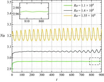
. This oscillating flow occurs between the laminar and turbulent regimes, corresponding to a Hopf bifurcation induced by elasticity. It is evident that elasticity significantly lowers the critical threshold, leading to a transition from stable to oscillatory natural convection at smaller Rayleigh numbers. This interesting phenomenon will be explored in § 4.3. To better understand the impact of viscosity ratios on steady-state flow, we fix
 $\xi = 2$
and
 $\lambda _{max} = 4$
.
Velocity field and streamlines at (a)
 $\beta = 0.1$
, (b)
 $\beta = 0.3$
, (c)
 $\beta = 0.5$
and (d)
 $\beta = 0.9$
. The other parameters are
 $Ra = 10^6$
,
 $Wi = 100$
,
 $\xi = 2$
and
 $\lambda _{max} = 4$
.

The streamlines along with the magnitude of the velocity field for Rolie-Poly fluids at different values of
 $\beta$
are presented in figure 12. When
 $\beta = 0.9$
, the contribution of the polymers is so minimal that the polymer solution behaves similarly to a Newtonian fluid, resulting in a flow structure akin to that observed in figure 5(c). As
 $\beta$
decreases to
 $0.5$
, a recirculation region begins to develop in the centre of the cavity and starts being drawn in the
 $x$
direction, forming vortex regions on both sides of the cavity. Ultimately, this recirculation region transforms into a parallel double vortex structure, as illustrated in figure 12(c). This microstructure can be visualised as two vortex regions connected by a finitely extensible spring. At
 $\beta = 0.3$
, this trend becomes even more pronounced, with the central spring being pulled longer, as depicted in figure 12(b). This occurs because the shear-thinning effect and the elastic properties of the polymer solution become more significant with increasing polymer concentration. The first normal stress tends to stretch the polymer chains in the
 $x$
direction (Peng et al. Reference Peng, Li, Xiong, Xu and Yu2021), especially as
 $\lambda _{max}$
is fixed at a smaller value of
 $4$
. Figure 13 illustrates the contour of
 $l$
for different values of
 $\beta$
, corresponding to the results shown in figure 12. The areas enclosed by the black curve represent the vortex regions. The length
 $l$
indicates the current length of the tube occupied by an entangled segment of the polymer, calculated as
 $l = \sqrt {\textrm {tr} (\boldsymbol{\sigma })}$
(Kabanemi & Hétu Reference Kabanemi and Hétu2009). It is evident that the stretching of the polymer’s entangled segments around the vortex regions and near the solid wall becomes more pronounced as the value of
 $\beta$
decreases, aligning with our previous analysis. As
 $\beta$
continues to decrease, the apparent viscosity of the polymer solution drops to a minimum due to the increasing effect of shear-thinning. As shown in figure 12(a), the two vortex structures in the middle of the cavity gradually merge into a single vortex structure, resulting in an increase in the size of the vortex region. Furthermore, the magnitude of the velocity field rises as
 $\beta$
decreases. It is noteworthy that the streamlines near the corners of the cavity become significantly distorted at
 $\beta = 0.1$
, indicating that buoyancy-induced convection plays a critical role in these areas. This suggests that local heat transfer in these regions may be greatly enhanced. We will verify this through analysis of the local and average Nusselt numbers in the following sections.
Contours of
 $l$
at (a)
 $\beta = 0.1$
, (b)
 $\beta = 0.3$
, (c)
 $\beta = 0.5$
and (d)
 $\beta = 0.9$
. The other parameters are
 $Ra = 10^6$
,
 $Wi = 100$
,
 $\xi = 2$
and
 $\lambda _{max} = 4$
.

Distribution of vertical and horizontal velocity components along the horizontal and vertical mid-planes of the cavity, respectively, at
 $Ra = 10^6$
. The other parameters are
 $Wi = 100$
,
 $\xi = 2$
and
 $\lambda _{max} = 4$
.

Figures 14(a) and 14(b) illustrate the changes in the vertical and horizontal velocity components along the horizontal and vertical mid-planes, respectively, of the cavity for different values of
 $\beta$
. As
 $\beta$
gradually decreases, the magnitude of both the maximum and minimum values of the velocity components increase significantly. At
 $\beta =0.1$
, the variation of the
 $u$
component along the vertical mid-planes shows a distortion that deviates from the original trend. This distortion is related to the phenomenon depicted in figure 12(a), where the streamlines become more distorted near the area above the left sidewall and below the right sidewall.
However, we set
 $Wi = 100$
and
 $\beta = 0.5$
to investigate the effect of the relaxation time ratio and fixed maximum stretch ratio. Initially, we fix
 $\lambda _{max} = 10$
and focus on the impact of
 $\xi$
. The streamlines and the magnitude of the velocity field are presented in figure 15 for Rolie-Poly fluids at different values of
 $\xi$
, where the result of
 $\xi = 1$
is shown in figure 9(i). At
 $\xi = 5$
, a two-vortex region forms in the centre of the cavity, connecting with vortex regions on both sides. This is illustrated in figure 15(d). As
 $\xi$
decreases to
 $2$
, the two-vortex region disappears, and the vortex regions on either side of the cavity are observed to stretch in a counterclockwise direction. When
 $\xi = 1$
, a single-vortex region is ultimately developed in the centre of the cavity. As
 $\xi$
further decreases, figures 15(a) and 15(b) show that the size of the recirculation region gradually increases. However, the reason for this trend differs from the previous analysis, where the enhancement of the shear-thinning effect promoted the formation of vortex regions. In the analysis of steady shear viscosity presented in figure 4(a), we observe that the steady-state shear viscosity of the Rolie-Poly model increases as
 $\xi$
decreases. This indicates that the shear-thinning effect diminishes with a lower value of
 $\xi$
. The increase in the apparent viscosity results in an enhanced damping effect from the viscous force, which gradually reduces the magnitude of the velocity field. It is important to note that both the steady extensional viscosity and the first normal stress difference become more pronounced as
 $\xi$
decreases. The first normal stress difference, which is related to stretching, primarily reflects the elasticity of the polymer microstructure. This relationship can be observed through the variation of specific elastic energy at different values of
 $\xi$
, as shown in figure 16. When stretch relaxation becomes the primary mechanism of stress relaxation, i.e. with a lower
 $\xi$
, elasticity becomes more significant. While the presence of extensional viscosity generally weakens the velocity gradient, the first normal stress tends to stretch the polymer chains in the
 $x$
direction. Consequently, despite the reduction in the velocity field due to increased apparent viscosity at lower values of
 $\xi$
, the lateral motion of the flow within the cavity is enhanced by the increased elasticity. This enhancement, in turn, facilitates the formation and development of the recirculation region.
Velocity field and streamlines at (a)
 $\xi = 0.2$
, (b)
 $\xi = 0.5$
, (c)
 $\xi = 2$
and (d)
 $\xi = 5$
. The other parameters are
 $Ra = 10^6$
,
 $Wi = 100$
,
 $\beta = 0.5$
and
 $\lambda _{max} = 10$
.

Variation of the specific elastic energy at
 $Ra = 10^6$
. The other parameters are
 $\beta = 0.5$
,
 $\xi = 1$
and
 $\lambda _{max} = 10$
.

Contours of the polymer normal stress
 ${\tau _p}_{xx}$
at (a)
 $\xi = 0.2$
, (b)
 $\xi = 1$
and (c)
 $\xi = 5$
. The other parameters are
 $Ra = 10^6$
,
 $Wi = 100$
,
 $\beta = 0.5$
and
 $\lambda _{max} = 10$
.

Figure 17 illustrates the distribution of polymer normal stress (
 ${\tau _p}_{xx}$
) within the square cavity. Stress concentrations appear near both the upper and lower walls, and this effect becomes more pronounced as
 $\xi$
decreases. The magnitude of the polymer normal stress increases significantly, indicating that the lateral movement of fluid along these walls has been notably enhanced. These observations align with our analysis. Additionally, there is a slight concentration of stress around the vortex regions, particularly when
 $\xi = 0.2$
. This phenomenon corresponds to the higher velocity magnitudes observed near the corners of the cavity along the upper and lower horizontal walls, as shown in figures 15(a) and 15(b). Figure 18 presents the variation of the vertical and horizontal velocity components along the horizontal and vertical mid-planes of the cavity, respectively, for different values of
 $\xi$
. The magnitude of the maximum or minimum value of
 $v$
shows a consistent increase with higher values of
 $\xi$
, as shown in figures 18(a) and 18(c). However, regardless of whether
 $\xi$
is less than
 $1$
or greater than
 $1$
, the magnitude of the maximum or minimum value of
 $u$
is smaller than it is at
 $\xi = 1$
, except for
 $\xi = 0.2$
. As illustrated in figure 18(b), the behaviour of
 $u$
along the vertical mid-plane of the cavity for
 $\xi = 0.2$
differs from that of the other values of
 $\xi$
, as the location of the maximum or minimum value of
 $u$
is positioned farther away from the sidewall.
Distribution of vertical and horizontal velocity components along the horizontal and vertical mid-planes of the cavity, respectively, at
 $Ra = 10^6$
. The other parameters are
 $Wi = 100$
,
 $\beta = 0.5$
and
 $\lambda _{max} = 10$
.

Velocity field and streamlines at (a)
 $\lambda _{max} = 4$
, (b)
 $\lambda _{max} = 7$
and (c)
 $\lambda _{max} = 10$
. The other parameters are
 $Ra = 10^6$
,
 $Wi = 100$
,
 $\beta = 0.5$
and
 $\xi = 1$
.

Next, we fix
 $\xi = 1$
to investigate the effect of
 $\lambda _{max}$
. We examine three cases:
 $\lambda _{max} = 4$
,
 $\lambda _{max} = 7$
and
 $\lambda _{max} = 10$
, which correspond to the scenarios of small, moderate and large stretching, respectively. Figure 19 illustrates the streamlines along with the magnitude of the velocity field for Rolie-Poly fluids at these different
 $\lambda _{max}$
values. As previously mentioned, the stretching of the polymer chain in the
 $x$
direction is most pronounced at
 $\lambda _{max} = 4$
. The two vortex regions in the centre of the cavity are drawn towards the
 $x$
direction, along with the vortex regions on either side of the cavity. This observation is generally consistent with our earlier findings, as depicted in figure 15(a). As
 $\lambda _{max}$
gradually increases, the two vortex regions begin to merge into a single vortex. The centre positions of the vortex regions on the left and right sides of the cavity shift downward and upward, respectively, while the overall size of the vortex region expands with increasing
 $\lambda _{max}$
. Figure 20 shows the variation of velocity components along the mid-plane of the cavity. The effect of
 $\lambda _{max}$
is evident solely in the horizontal velocity component, where the maximum or minimum value of
 $u$
increases as
 $\lambda _{max}$
increases.
Distribution of vertical and horizontal velocity components along the horizontal and vertical mid-planes of the cavity respectively at
 $Ra = 10^6$
. The other parameters are
 $Wi = 100$
,
 $\beta = 0.5$
and
 $\xi = 1$
.

Contours of
 $\lambda$
at (a)
 $\lambda _{max} = 4$
, (b)
 $\lambda _{max} = 7$
and (c)
 $\lambda _{max} = 10$
. The other parameters are
 $Ra = 10^6$
,
 $Wi = 100$
,
 $\beta = 0.5$
and
 $\xi = 1$
.

The extended Rolie-Poly model, in contrast to the original model, takes into account the finite extensibility of polymers, which limits their degree of strain hardening in strong stretching conditions (Kabanemi & Hétu Reference Kabanemi and Hétu2009). Figure 21 shows the contour of
 $\lambda$
for different
 $\lambda _{max}$
values, corresponding to the results presented in figure 19. The areas enclosed by the black curve represent the corresponding vortex regions. As noted,
 $\lambda$
denotes the ratio of polymer chain stretch. It is evident that the stretch ratio in each area is less than the fixed maximum stretch ratio. Additionally, the stretch ratio around the vortex regions is closer to the fixed maximum stretch ratio compared with the stretch ratio within the vortex region, especially when
 $\lambda _{max} = 4$
. This observation suggests that the areas surrounding the vortex regions experience a higher velocity gradient. Furthermore, the stretch ratio near the walls of the cavity is also significant, with the maximum stretch ratio typically occurring at the corners of the cavity. This finding aligns with previous analyses indicating that the flow induced by buoyancy moves relatively quickly along the cavity walls, as illustrated in figure 6.
4.2. Dependence of heat transport on the parameters
4.2.1. Nusselt number
In this subsection, we examine how heat transfer depends on various control parameters and quantify heat transfer performance using the Nusselt number. Figure 22 shows the local heat transfer rate along the left vertical hot wall for both Newtonian and Rolie-Poly fluids. At
 $Ra = 10^3$
, the distribution of
 $Nu_l$
appears flat, indicating weak convection. Consequently, there is little significant difference between the heat transfer performance of Newtonian and Rolie-Poly fluids at this stage. As the Rayleigh number gradually increases, a notable difference begins to emerge at
 $Ra=10^5$
. Here,
 $Nu_l$
slightly increases near the bottom corner of the cavity before gradually decreasing, ultimately reaching its minimum at the top corner. This pattern occurs because the thickness of the thermal boundary layer increases from the bottom corner to the top, as illustrated by the isothermal patterns in figure 8. The local thermal boundary layer detaches from the surface near the bottom of the left hot wall in the form of plumes, which enhances local heat transfer (Cheng et al. Reference Cheng, Cai, Zhang, Li, Shen, Yu and Qian2019). This trend becomes even more pronounced at
 $10^6$
, where heat transfer is predominantly driven by convection. Due to the effect of the shear-thining effect, the maximum value of
 $Nu_l$
for Rolie-Poly fluid near the bottom corner of the cavity is significantly higher than that of the Newtonian fluid, increasing by approximately
 $28.7\,\%$
. The black dashed line shows the position of the maximum
 $Nu_l$
in relation to the Rayleigh number. As the Rayleigh number increases, this position gradually moves closer to the wall, which means that the thermal plume can more easily separate from the thermal boundary layer.
Distribution of
 $Nu_l$
along the left vertical hot wall of the cavity for Newtonian and Rolie-Poly fluids. The red bullets mark the the position of the maximum
 $Nu_l$
. The other parameters are
 $Wi = 10$
,
 $\beta = 0.5$
,
 $\xi = 1$
and
 $\lambda _{max} = 10$
.

Distribution of
 $Nu$
versus
 $Ra$
for Newtonian and Rolie-Poly fluids. The other parameters are
 $Wi = 10$
,
 $\beta = 0.5$
,
 $\xi = 1$
and
 $\lambda _{max} = 10$
.

For the average heat transfer rate, from figure 23, we see that the
 $Nu$
scaling is
 $Nu \sim Ra^{0.27035}$
, which is close to
 $Nu \sim Ra^{1/4}$
corresponding to the laminar scaling for classical RBC (Grossmann & Lohse Reference Grossmann and Lohse2000). Although the
 $Nu$
scale is slightly higher than
 $Ra^{1/4}$
, it still aligns with the laminar scaling governed by boundary layer dissipation like
 $Ra^{\gamma }$
(with
 $0.245 \lt \gamma \lt 0.287$
) (Toppaladoddi & Wettlaufer Reference Toppaladoddi and Wettlaufer2018). In comparison to the Newtonian fluids, the Rolie-Poly fluids with weak elasticity exhibit the same scaling law for
 $Nu$
, with the presence of the polymer increasing the magnitude of
 $Nu$
. However, this behaviour changes in scenarios with strong elasticity, which will be analysed in § 4.3. Moreover, we note that the
 $Nu$
scaling does not strictly follow
 $Nu \sim Ra^{0.27035}$
for either Newtonian or Rolie-Poly fluids at lower
 $Ra$
, as shown in the photomicrographs of figure 23. In the regime of
 $10^3 \leqslant Ra \leqslant 10^6$
, the thickness of the stable layer, which is dominated by viscous dissipation, is greater. This results in a higher
 $Nu$
scaling during the early stages of convective development (Toppaladoddi & Wettlaufer Reference Toppaladoddi and Wettlaufer2018).
We examine how elasticity affects heat transport by fixing the Rayleigh number to
 $Ra = 10^3$
and
 $Ra = 10^6$
. When convective intensity is weak, meaning the inertial effects are minimal, the influence of elasticity becomes more pronounced. The cases examined include:
 $Wi = 1$
with
 $\lambda _{max} = 4$
,
 $Wi = 10$
with
 $\lambda _{max} = 4$
,
 $Wi = 50$
with
 $\lambda _{max} = 10$
and
 $Wi = 100$
with
 $\lambda _{max} = 10$
. These correspond to the scenarios of weak elasticity with a small stretch ratio, moderate elasticity with a large stretch ratio and strong elasticity with a large stretch ratio. For oscillating flow (
 $\beta \leqslant 0.4$
), the average Nusselt number is given as its time-averaged value. Figure 24 shows the average Nusselt number for various scenarios plotted against
 $\beta$
at
 $Ra = 10^3$
and
 $Ra = 10^6$
. Compared with in Newtonian fluids, polymers enhance heat transfer in different scenarios due to the shear-thinning effect, even with a minimal polymer contribution at
 $\beta = 0.9$
. As
 $\beta$
gradually decreases, the enhancement in heat transfer increases rapidly. At
 $Ra = 10^3$
, the
 $Nu$
for
 $Wi = 10$
is similar to that of Newtonian fluids due to weak elasticity. As the Weissenberg number increases,
 $Nu$
initially rises significantly and then reaches a maximum value at
 $Wi =50$
, after which it gradually decreases at
 $Wi =100$
, as shown in figure 24(a). The maximum
 $Nu$
at
 $Wi = 50$
is approximately
 $41.5\,\%$
higher than that of Newtonian fluids at
 $\beta = 0.1$
. This non-monotonic trend of
 $Nu$
aligns with the observed relationship between the velocity field and Weissenberg number, as described in § 4.1.2.
Distribution of
 $Nu$
versus
 $\beta$
for different scenarios at (a)
 $Ra = 10^3$
and (b)
 $Ra = 10^6$
with
 $\xi = 1$
.

Distribution of
 $Nu_l$
along the left vertical hot wall of the cavity at
 $Ra = 10^6$
. The red bullets mark the the position of the maximum
 $Nu_l$
. The other parameters are
 $Wi = 10$
,
 $\beta = 0.5$
and
 $\xi = 1$
.

Figure 25 illustrates the distribution of
 $Nu_l$
for different values of
 $\lambda _{max}$
. It can be observed that as
 $\lambda _{max}$
increases, the heat transfer tends to improve. However, this enhancement is localised and occurs primarily in the vicinity of the maximum
 $Nu_l$
. Consequently, the impact of
 $Wi$
on heat transfer is more significant than that of
 $\lambda _{max}$
. As the Rayleigh number increases to
 $10^6$
, the average Nusselt number for
 $Wi = 1$
is significantly higher than that of Newtonian fluids, owing to the enhancement of buoyancy-induced convection, as shown in figure 24(b). The Nusselt number values for
 $Wi = 10$
and
 $Wi = 100$
are very similar, but they still exhibit the same non-monotonic trend observed at
 $Ra = 10^3$
. Notably, the maximum
 $Nu$
for
 $Wi = 50$
reaches approximately
 $64.9\,\%$
compared with Newtonian fluids at
 $\beta = 0.1$
.
Distribution of
 $Nu$
versus
 $Wi$
at (a)
 $Ra = 10^3$
and (b)
 $Ra = 10^6$
. The other parameters are
 $\beta = 0.5$
and
 $\lambda _{max} = 10$
.

We further investigate the effects of the relaxation time ratio and Weissenberg number on heat transport, as shown in figure 26. It is evident that
 $Nu$
increases as
 $\xi$
gradually increases. This might imply that the enhancement of heat transfer in Rolie-Poly fluids is more significant when orientation relaxation becomes the main mechanism for stress relaxation. From the perspective of rheological analysis in § 3, the shear-thinning effect becomes more pronounced, while the elastic properties gradually decrease as the value of
 $\xi$
increases. This indicates that the shear-thinning effect of polymer tends to promote heat transfer, while their elastic properties may hinder it. Moreover, the heat transfer enhancement due to changes in
 $\xi$
varies at different Weissenberg numbers. For instance, see figure 26(a),
 $Nu$
increases by
 $11\,\%$
at
 $Wi = 20$
when
 $\xi$
rises from
 $0.2$
to
 $5$
. In contrast, the corresponding enhancement is
 $17\,\%$
at
 $Wi = 100$
.
However, the effect of the Weissenberg number on heat transfer is more complicated. At
 $Ra = 10^3$
,
 $Nu$
initially increases rapidly with
 $Wi$
up to a critical value, after which it either remains nearly constant or decreases slightly, as shown in figure 26(a). This critical
 $Wi$
, where the transition occurs, tends to increase gradually as the parameter
 $\xi$
increases. Interestingly, at
 $\xi = 0.2$
, the
 $Nu$
is slightly lower than that of Newtonian fluids. This suggests that the addition of polymers does not always enhance the heat transfer, and in cases where the convective intensity is weak (with lower
 $\xi$
), heat transfer may actually decrease. This behaviour is primarily due to the apparent viscosity of the polymer solution, which is highly dependent on
 $Wi$
and tends to decrease as
 $Wi$
increases. On the one hand, the shear-thinning effect of the polymer solution promotes heat transfer; on the other hand, the elastic properties of the polymer solution also increase with rising
 $Wi$
, which can hinder heat transfer. Therefore, at any given Weissenberg number, the heat transfer rate in Rolie-Poly fluid is influenced by the competition between the shear-thinning effect and the elastic properties. Before reaching the critical value of
 $Wi$
, the shear-thinning effect predominates over the elastic properties, leading to an enhancement in heat transfer. However, once this critical value is surpassed, the elastic properties become more significant and may dominate over the shear-thinning effect. Consequently, the heat transfer rate remains nearly constant or begins to decline. The maximum value of
 $Nu$
occurs at
 $Wi = 80$
, showing an increase of approximately
 $16.1\,\%$
compared with Newtonian fluids.
As the Rayleigh number increases to
 $10^6$
, the average Nusselt number significantly increases due to the increase in the buoyancy-induced convection. As illustrated in figure 26(b), the maximum
 $Nu$
is observed at
 $Wi = 100$
with
 $\xi = 5$
, representing an increase of approximately
 $20.8\,\%$
compared with Newtonian fluids. The heat transfer reduction observed at
 $Ra = 10^3$
disappears, while
 $Nu$
shows a slight upward trend as
 $Wi$
rises from
 $50$
to
 $100$
at
 $\xi = 0.2$
. This non-monotonic behaviour may be linked to the loss of monotonicity at high shear rates for
 $\xi = 0.2$
, as described in figure 4(a). This phenomenon becomes more pronounced in the strong elasticity scenario, which will be analysed in § 4.3.2.
4.2.2. Boundary layer analysis
To better understand these heat transfer performances, we investigate the boundary layers in the same scenarios, both thermal and viscous. Previous studies on the RBC system have proposed several methods for defining boundary layer thickness (Ahlers, Grossmann & Lohse Reference Ahlers, Grossmann and Lohse2009; Scheel, Kim & White Reference Scheel, Kim and White2012). In this work, we adopt the method that uses the slopes of velocity and temperature distributions to determine the viscous BL and thermal BL thickness, respectively. For the thermal BL thicknesses, we introduce a dimensionless temperature,
 $\theta '$
, as follows (Su et al. Reference Su, Li, Luo, Wu and Yi2021):
 \begin{align} \theta ' = \frac {T_1-T}{(T_1-T_0)/2}. \end{align}
For the viscous BL thickness, it is essential to find the maximum velocity
 $U_{max}$
, near both the top and bottom of the boundary layer. This is because the linear fit of the velocity profile intersects with this maximum value close to the boundary (Cheng et al. Reference Cheng, Zhang, Cai, Li and Li2017). Hence, we define a dimensionless velocity,
 $U'$
, as follows:
 \begin{align} U' = \frac {U}{U_{max}}, \end{align}
where
 $U = \sqrt {u^2 + v^2}$
is the magnitude of velocity field.
Profiles of (a)
 $\theta ' (x)$
and (b)
 $U' (y)$
respectively along the horizontal and vertical centreline of the cavity both for Newtonian fluid and Rolie-Poly fluid at
 $Ra = 10^6$
. The other parameters are
 $\beta = 0.5$
,
 $\xi = 1$
and
 $\lambda _{max} = 10$
. The inclined straight lines have a linear dependence with
 $\theta ' (x)$
and
 $U' (y)$
profiles. The abscissas are normalised by
 $\lambda _{th}$
and
 $\lambda _{v}$
, respectively.

As an example, the dimensionless temperature
 $\theta ' (x)\mid _{y = 1/2}$
and the dimensionless velocity
 $U' (y)\mid _{x = 1/2}$
profiles are plotted respectively along the horizontal and vertical centreline of the cavity, as shown in figure 27, both for Newtonian fluids and Rolie-Poly fluids. The distance is normalised by the thickness of thermal BL (
 $\lambda _{th}$
) and viscous BL (
 $\lambda _{v}$
). As shown in figure 27(a),
 $\lambda _{th}$
is the distance from the left hot sidewall to the position at which the extrapolation of the linear part of
 $\theta ' (x)$
profile crosses the isoline determined by the bulk temperature. Additionally,
 $\lambda _{v}$
is obtained by a similar method, as shown in figure 27(b), where the linear part of
 $U' (y)$
profile intersects with the isoline defined by
 $\langle U (y) \mid _{x = 1/2} \rangle _{max}$
. In this case,
 $\lambda _{th}$
and
 $\lambda _{v}$
in the Newtonian fluid are calculated to be
 $0.0586$
and
 $0.0467$
, respectively.
Thermal BL thickness and viscous BL thickness versus
 $\beta$
at (a)
 $Ra = 10^3$
and (b)
 $Ra = 10^6$
with
 $\xi = 1$
.

Figure 28 illustrates the thermal and viscous BL thickness in the scenarios characterised by weak elasticity with a small stretch ratio and moderate elasticity with a large stretch ratio. These scenarios correspond to the maximum and minimum enhancements in heat transfer caused by the polymers, as shown in figure 24. The trend of
 $\lambda _{th}$
across all scenarios generally agrees with the corresponding heat transfer performance. This indicates that the thermal BLs for the lower
 $\beta$
cases are indeed thinner and more unstable.
For the viscous BLs, a similar trend to
 $\lambda _{th}$
is observed, indicating that kinetic energy and heat transfer mutually reinforce each other. In the case of
 $Wi = 1$
with
 $\lambda _{max} = 4$
, as
 $\beta$
gradually decreases,
 $\lambda _{v}$
significantly decreases at
 $Ra = 10^3$
, while it only slightly decreases at
 $Ra = 10^6$
. This observation can be understood as the influence of polymers on viscous BLs in the weak elasticity scenario is clear when the inertial effects are minimal (indicating weak convective intensity) at
 $Ra = 10^3$
. As
 $Ra$
increases to
 $Ra = 10^6$
, the elastic effect diminishes due to the dominance of inertia. In contrast, for
 $Wi = 50$
with
 $\lambda _{max} = 10$
,
 $\lambda _{v}$
remains almost unchanged for
 $\beta \geqslant 0.4$
at
 $Ra = 10^3$
, and then gradually decreases for
 $\beta \lt 0.4$
. When
 $Ra = 10^6$
,
 $\lambda _{v}$
begins to decrease at
 $\beta = 0.9$
as
 $\beta$
continues to decrease. This means that the influence of polymers in moderate and strong elasticity scenarios is motivated when the convective intensity is strong enough.
Thermal BL thickness and viscous BL thickness versus
 $Wi$
at (a)
 $Ra = 10^3$
and (b)
 $Ra = 10^6$
. The other parameters are
 $\beta = 0.5$
and
 $\lambda _{max} = 10$
.

Figure 29 presents the viscous BL and thermal BL thickness as a function of
 $Wi$
for different values of
 $\xi$
. These align with the cases considered in the heat transfer performance, as shown in figure 26. Similar to the trend observed in
 $Nu$
,
 $\lambda _{th}$
initially decreases significantly until
 $Wi$
reaches a critical value, after which it increases slightly. Moreover,
 $\lambda _{th}$
gradually decreases as
 $\xi$
increases. Notably, for
 $\xi = 0.2$
,
 $\lambda _{th}$
is higher than that of the Newtonian fluid at
 $Wi = 80$
when
 $Ra = 10^3$
. This finding corresponds to the stage of HTR in figure 26(a). These observations provide a direct explanation for HTE or HTR caused by the polymer additives within thermal BLs.
Compared with
 $\lambda _{th}$
at
 $Ra = 10^3$
,
 $\lambda _{v}$
demonstrates a similar trend: it first drops slightly with increasing
 $Wi$
up to a critical value and then gradually increases. Additionally,
 $\lambda _{v}$
is consistently thicker than that of Newtonian fluids for all
 $\xi$
when
 $Wi \geqslant 80$
, particularly for
 $\xi = 0.2$
. This observation can be interpreted as a further indication of the decrease in heat transfer rate. As
 $Ra$
increases to
 $Ra = 10^6$
, the variation of
 $\lambda _{v}$
with
 $Wi$
resembles that of
 $\lambda _{th}$
. However, the influence of
 $\xi$
on the viscous BLs is unexpected. We observe that
 $\lambda _{th}$
gradually decreases as
 $\xi$
increases, while
 $\lambda _{v}$
increases. This indicates that the heat transport is enhanced with increasing
 $\xi$
, while the kinetic energy decreases. As illustrated in figure 15, the maximum value of the velocity field gradually increases with rising
 $\xi$
, suggesting that the kinetic energy indeed increases as
 $\xi$
does. It follows that the greater the kinetic energy and the better the heat transport, the thinner will be the corresponding
 $\lambda _{th}$
. This raises the question: Why does
 $\lambda _{v}$
vary differently? It is important to note that the viscous BLs discussed here refer to the bottom wall of the cavity, not the left hot wall. Reviewing § 4.1.2, we suggest that the lateral motion of the polymer solution is accelerated in the
 $x$
direction as
 $\xi$
decreases. This correlation, with
 $\lambda _{v}$
decreasing as
 $\xi$
decreases, supports our analysis.
4.2.3. Kinetic energy budget
To assist in analysing the heat transfer performance caused by the elastic effect, we introduce the kinetic energy budget equation for the natural convection of Rolie-Poly fluid. The performance of heat transport in various scenarios is linked to fluid motion. Polymer additives have a direct impact on the development of the velocity field, which can either enhance or hinder heat transport. Consequently, analysing the kinetic energy budget provides an additional perspective for understanding heat transport.
The dimensionless elastic stress
 $\boldsymbol{\tau }_p$
is expressed as
 \begin{align} \boldsymbol{\tau }_p = \frac {1 - \beta }{Wi} k_s(\lambda ) (\boldsymbol{\sigma } - \boldsymbol{I}). \end{align}
We consider the dot product of (2.11) and
 ${1}/{2}\boldsymbol{u}$
, so by combining (4.5), the equilibrium equation of instantaneous kinetic energy is derived as follows (Cheng et al. Reference Cheng, Cai, Zhang, Li, Shen, Yu and Qian2019):
 \begin{align} \frac {\textrm {d} E_u}{\textrm {d} t} = D + F + V + G, \end{align}
where
 $E_u = {1}/{2} \boldsymbol{u} \cdot \boldsymbol{u}$
is the global kinetic energy;
 $D = \nabla \cdot (p\boldsymbol{u} + {\beta }/{\sqrt {Ra/Pr}} \nabla E_u + {1}/{\sqrt {Ra/Pr}}\boldsymbol{u} \cdot \boldsymbol{\tau }_p)$
denotes the kinetic diffusion;
 $F = \theta v$
is the input of thermal energy;
 $V = - {\beta }/{\sqrt {Ra/Pr}}(\nabla \boldsymbol{u} : \nabla \boldsymbol{u})$
represents the viscous dissipation of kinetic energy. Finally,
 $G = -(1 - \beta) / (Wi \sqrt{Ra/Pr} ) k_s(\lambda) \left[ ( \boldsymbol{\sigma} - \boldsymbol{I}) : \nabla \boldsymbol{u} \right]$
stands for the energy exchange between the flow structures and polymer microstructures caused by the stretch and relaxation of polymer chains in the flow. When the energy exchange term
 $G\lt 0$
, the energy of the flow structures is absorbed into the microstructures of the entangled polymer.
A spatial average over the whole field can be defined as follows, respectively:
 \begin{eqnarray} \bar {D} = \frac {1}{A} \int _{\Omega } D \textrm {d}\textrm {S}, \quad \bar {F} = \frac {1}{A} \int _{\Omega } F \textrm {d}\textrm {S}, \quad \bar {V} = \frac {1}{A} \int _{\Omega } V \textrm {d}\textrm {S},\quad \bar {G} = \frac {1}{A} \int _{\Omega } G \textrm {d}\textrm {S}, \end{eqnarray}
where
 $A$
is the whole area. Here,
 $\bar {D}$
is zero due to the nature of diffusion term in a closed system (Cheng et al. Reference Cheng, Zhang, Cai, Li and Li2017).
Kinetic energy budget versus
 $\beta$
at (a)
 $Ra = 10^3$
and (b)
 $Ra = 10^6$
with
 $\xi = 1$
.

Figure 30 illustrates the kinetic energy budget for both Newtonian and Rolie-Poly fluids versus
 $\beta$
. We observe that the variation of each term at
 $Ra = 10^3$
resembles that at
 $Ra = 10^6$
. As with Newtonian fluids, the term
 $\bar {F}$
, which represents the energy input from thermal energy, is always positive in Rolie-Poly fluids, while
 $\bar {V}$
consistently serves as the energy sink and remains negative. As
 $\beta$
gradually decreases,
 $\bar {F}$
increases across all scenarios, indicating that the presence of polymer additives enhances the input of thermal energy. Specifically, in the case of
 $Wi = 1$
with
 $\lambda _{max} = 4$
,
 $\bar {F}$
exhibits only a slight increase at
 $Ra = 10^3$
as
 $\beta$
decreases, but a significant increase at
 $Ra = 10^6$
. This observation aligns well with the corresponding trends of
 $Nu$
and
 $\lambda _{th}$
, further demonstrating that kinetic energy and heat transfer mutually reinforce each other. In the context of viscous dissipation of kinetic energy, weak elasticity and moderate elasticity scenarios exhibit distinct behaviours. In the case of
 $Wi = 1$
with
 $\lambda _{max} = 4$
, the magnitude of
 $\bar {V}$
gradually decreases as the parameter
 $\beta$
lowers, ultimately becoming smaller than that observed in Newtonian fluids. Conversely, for
 $Wi = 50$
with
 $\lambda _{max} = 10$
, the magnitude of
 $\bar {V}$
initially experiences a slight drop before gradually increasing as
 $\beta$
decreases, remaining larger than that of Newtonian fluids. This intriguing phenomenon suggests that, in weak elasticity scenarios with a small stretch ratio, polymers can significantly reduce viscous dissipation.
Furthermore,
 $\bar {G}$
is negative, similar to
 $\bar {V}$
, indicating that a portion of the energy is transferred from the flow structures into the polymer microstructures. This behaviour is also observed in wall-bounded flows, leading to TDR due to the stretching of polymers (Cai, Li & Zhang Reference Cai, Li and Zhang2010). As
 $\beta$
decreases, the magnitude of
 $\bar {G}$
increases, which is attributed to an increase in elasticity. We find that the magnitude of
 $\bar {G}$
for
 $Wi = 1$
is consistently greater than that for
 $Wi = 50$
at
 $Ra = 10^6$
. This suggests that, in the case of weak elasticity with a small stretch ratio, more energy is stored in the polymer microstructures. However, the energy analysis indicates that the elastic energy
 $E_e$
gradually increases with increasing
 $Wi$
, as shown in figure 10. It is important to note that the maximum stretch ratio (
 $\lambda _{max}$
) is a critical parameter in determining the degree of polymer stretching. A smaller
 $\lambda _{max}$
allows for easier stretching of the polymer chain. Thus, more energy is stored in the polymer microstructures for the case of
 $Wi$
with
 $\lambda _{max} = 4$
, despite the lower elasticity.
Kinetic energy budget versus
 $Wi$
at (a)
 $Ra = 10^3$
and (b)
 $Ra = 10^6$
. The other parameters are
 $\beta = 0.5$
and
 $\lambda _{max} = 10$
.

Figure 31 illustrates the kinetic energy budget for both Newtonian and Rolie-Poly fluids versus
 $Wi$
for different values of
 $\xi$
. At
 $Ra = 10^3$
, as
 $Wi$
gradually increases,
 $\bar {F}$
initially rises significantly before stabilising at a nearly constant level, as shown in figure 31(a). It roughly corresponds with the observed behaviours of
 $Nu$
and
 $\lambda _{th}$
, highlighting the competition between the shear-thinning effect and elasticity. Similarly, the viscous dissipation of kinetic energy (
 $\bar {V}$
) also shows an increasing trend with
 $Wi$
, indicating that elasticity contributes to this dissipation. However,
 $\bar {G}$
remains negative and its magnitude gradually diminishes as
 $Wi$
increases. During this process,
 $\bar {G}$
acts as an energy source, along with
 $\bar {F}$
, to release energy into the flow structures. This behaviour differs when
 $\beta$
increases, despite a fundamental increase in elasticity.
Contours of
 $G$
at (a)
 $Wi = 1$
, (b)
 $Wi = 20$
and (c)
 $Wi = 100$
at
 $Ra = 10^3$
. The other parameters are
 $\beta = 0.5$
,
 $\xi = 1$
and
 $\lambda _{max} = 10$
.

To better understand this process, figure 32 illustrates the spatial distribution of
 $G$
for different values of
 $Wi$
. The areas where
 $G \gt 0$
are highlighted in red. The red areas increase significantly as
 $Wi$
rises from
 $1$
to
 $20$
. This indicates that the energy exchange from the polymers to the flow structures is increasing, even though the overall energy remains stored in the polymer microstructures. This observation aligns with our analysis and provides direct evidence of this process. Notably, the red areas first appear in the regions of the vortices, indicating that the flow structure becomes more complex at that point.
However, we focus on the effect of
 $\xi$
on the kinetic energy budget. It is observed that the influence of
 $\xi$
on each term is monotonic when
 $Ra = 10^3$
. As
 $\xi$
increases,
 $\bar {F}$
increases and the magnitude of
 $\bar {G}$
decreases. This change corresponds to the increase in the velocity field with
 $\xi$
, as shown in figure 15, since
 $\bar {G}$
acts as an energy source alongside
 $\bar {F}$
in this process. For
 $\xi = 0.2$
, the magnitude of
 $\bar {G}$
is greater than that for
 $\xi = 5$
, which can be attributed to the stretching of the polymer, further indicating the dominance of stretch relaxation. Additionally, the magnitude of
 $\bar {V}$
, the only energy sink, also increases. Unlike the weak elasticity stage, polymer additives significantly increase viscous dissipation during the strong elasticity stage (
 $Wi \gt 10$
), as the orientation relaxation gradually becomes the main mechanism for stress relaxation when
 $\xi \geqslant 1$
. As the Rayleigh number increases to
 $10^6$
, the overall trend of each term as a function of
 $Wi$
remains similar to that of
 $Ra = 10^3$
. Comparing figures 31(a) and 31(b), it is evident that the magnitude of each term at
 $Ra = 10^6$
is much smaller than that at
 $Ra = 10^3$
, suggesting that the cases at this Rayleigh number are dominated by inertia due to the increase in convective intensity. Moreover, the loss of monotonicity for
 $\bar {F}$
with respect to
 $\xi$
also further confirms this trend.
4.3. Bifurcation
In § 4.1.2, we observe an oscillatory flow in scenarios with strong elasticity as the polymer solution gradually approaches the melt state. This behaviour corresponds to an Hopf bifurcation in two-dimensional natural convection. As the Rayleigh numbers increase, all convective flows eventually become turbulent, with oscillatory flows typically situated between laminar and turbulent states. However, for the natural convection of Newtonian fluids in a differentially heated square cavity, the critical Rayleigh number is notably high. Interestingly, the bifurcation observed in Rolie-Poly fluids tends to occur at lower Rayleigh numbers. The elasticity significantly lowers the instability threshold for convection. This phenomenon is reminiscent of the non-inertial elastic turbulence identified in viscoelastic parallel shear flows (Morozov & van Saarloos Reference Morozov and van Saarloos2007). In this type of flow, the nonlinear effects typically arise not from inertial terms, but from elastic terms due to small driving parameters. To further investigate this behaviour, we conducted direct numerical simulations to examine the transitions from laminar to turbulent flow driven by both inertia (buoyancy) and elasticity, respectively.
4.3.1. Driven by inertia
In classic Rayleigh–Bénard convection, the flow becomes unstable from a static conductive state only when the Rayleigh number exceeds a certain critical value. This phenomenon can be described as an exchange of stability occurring at the critical Rayleigh number, where the stability of the stationary state is transitioned to the stability of the flowing state (Bergé & Dubois Reference Bergé and Dubois1984). For reasons of symmetry, the descending motion of denser fluid elements has the same probability of occurring as the ascending motion of less dense fluid elements. Therefore, the onset of Rayleigh–Bénard convection experiences a bifurcation with two symmetrical branches. However, this behaviour contrasts with natural convection in a differentially heated cavity when the temperature gradient is horizontal. In this configuration, the flow becomes unstable immediately and there is no threshold for natural convection. This is because there is inherently upward movement at the hot plate and downward movement at the cold plate.
To gain more detailed insights into the bifurcations, we study the long-term behaviour at Rayleigh numbers near the bifurcation points. We use numerical solutions under specific initial conditions as the fundamental flow to calculate results and wait for the flow to reach a stable state. This process allows us to determine the physically stable branches of the bifurcation diagram. We conclude that bifurcation has occurred based on the observation that the equilibrium time increases significantly as we approach the critical point (Paolucci & Chenoweth Reference Paolucci and Chenoweth1989). The characteristics of the solution change markedly at this juncture, which is evident in the Fourier frequency spectrum.
We begin our numerical simulation at
 $Ra = 10^3$
and gradually increase the convective intensity up to
 $Ra = 10^5$
. The average Nusselt number
 $Nu$
is used as the primary metric to distinguish between flow states. Figure 33 illustrates the relationship between time-averaged
 $Nu$
and
 $Ra$
for Rolie-Poly fluids at
 $Wi = 100$
within the strong elasticity scenarios. The four stages of convection are marked in different colours to represent distinct regions. As the inertia effects gradually increase, convection progresses through four stages, which correspond to the following regions: I, steady convection; II, periodic oscillatory convection; III, quasi-periodic oscillatory convection; IV, chaotic convection. This observation aligns with the long-term behaviour predicted in the qualitative theory of partial differential equations, where several paths, steady attractor, periodic attractor, quasi-periodic attractor and chaotic attractor, can be identified to influence the initial solution (Henkes & Hoogendoorn Reference Henkes and Hoogendoorn1990). Furthermore, heat transport follows a
 $Nu \sim Ra^{0.38198}$
scaling that is significantly higher than
 $Ra^{\gamma }$
(
 $0.245 \lt \gamma \lt 0.287$
). This result suggests that heat transfer is suppressed and that the thickness of the stable layer is greater under strong elasticity scenarios. This can be confirmed by observing that the thermal BL and the viscous BL thickness for
 $\xi = 0.2$
are thicker than those of a Newtonian fluid.
Distribution of
 $Nu$
versus
 $Ra$
at
 $Wi = 100$
. The other parameters are
 $\beta = 0.1$
,
 $\xi = 0.2$
and
 $\lambda _{max} = 10$
.

Temporal evolution of
 $Nu$
for
 $Wi = 100$
during early periodic flow.

The first critical Rayleigh number,
 $Ra_{c1}$
, at which the flow achieves a steady state in an oscillatory manner occurs at
 $11\,000$
. The flow is attracted to an oscillating solution and the characteristic quantity
 $Nu$
oscillates with the same frequency and amplitude. Figure 34 illustrates the temporal evolution of
 $Nu$
for
 $Wi = 100$
during the early stage of periodic oscillatory convection. At
 $Ra_{c1} = 11\,000$
, the amplitude of the oscillation is very small (as shown in the inset) when the flow first enters the periodic oscillation regime. As the inertia effect increases, the amplitude of the oscillation at
 $Ra = 14\,000$
significantly rises. Since the development of the instability is very slow near the critical Rayleigh number, the flow requires a long period to evolve into stable periodic oscillations.
Temporal evolution of
 $Nu$
at
 $Ra = 14\,000$
.

The complete temporal evolution of
 $Nu$
at
 $Ra = 14\,000$
is presented in figure 35. The flow gradually develops during the initial moments and ultimately reaches stable oscillatory convection through long-term evolution. As the Rayleigh number increases to
 $15\,500$
, the amplitude of oscillation continues to rise and quickly reaches a stable periodic state.
(a) Temporal evolution of
 $Nu$
and (b) corresponding Fourier spectra at
 $Ra = 16\,000$
. The symbols A–F correspond to values of time at which the spatial structures are given in figure 37, respectively.

Figure 36 illustrates the temporal evolution of
 $Nu$
at
 $Ra = 16\,000$
along with the corresponding Fourier spectra. The Nusselt number exhibits a fixed frequency (
 $f$
) and amplitude (
 $A_{Nu}$
) at
 $Ra = 16\,000$
, characteristic of periodic flow. The time series spectrum reveals a fundamental frequency of
 $0.0235$
, along with several higher harmonics that are integral multiples of this fundamental frequency. Figure 37 shows the spatial structures of the oscillatory flow at
 $Ra = 16\,000$
, corresponding to specific times throughout the period, labelled A–F in figure 36. During one complete oscillation, the vortex region rotates clockwise at the centre of the square cavity, indicating a change in the position of the vortex centre. It is important to note that there is a peak velocity area on each side of the square cavity, demonstrating an intriguing trend. When the centre of the vortex approaches the right wall, the peak velocity area on the left side increases, while that on the right side decreases. Conversely, when the centre of the vortex is closer to the left wall, the peak velocity regions on both sides exhibit opposite trends. This behaviour aligns with the oscillation of the vortex region. At the commencement of a new period, the spatial structure labelled F closely resembles that of label A, as illustrated in figures 37(a) and 37(f). Figure 38 depicts the temporal evolution of
 $Nu$
at
 $Ra = 17\,000$
and
 $Ra = 18\,000$
. As the Rayleigh number increases, the amplitude of
 $Nu$
also rises, while the dominant oscillation frequency remains unchanged. Some minor distortions can be observed in the trough region, as highlighted in the inset.
Velocity field and streamlines at
 $Ra = 16\,000$
: panels (a)–(f) correspond to time values A–F in figure 36.

Temporal evolution of
 $Nu$
at
 $Ra = 17\,000$
and
 $Ra = 18\,000$
.

Bifurcation diagram in the
 $Ra$
–
 $A_{Nu}$
plane with (a) increasing
 $Ra$
and (b) decreasing
 $Ra$
at
 $Wi = 100$
.

Time histories and Fourier spectra of
 $Nu$
at (a,b)
 $Ra = 21\,000$
and (c,d)
 $Ra = 30\,000$
.

The bifurcation diagram in the
 $Ra$
–
 $A_{Nu}$
plane with increasing
 $Ra$
is presented in figure 39(a). This diagram illustrates the characteristics of a classical Hopf bifurcation occurring at
 $Ra_{c1} = 11\,000$
. As the intensity of convection increases, the amplitude of the periodic oscillations sharpens significantly; however, during this stage, the flow maintains a single dominant frequency until reaching the second critical Rayleigh number. Starting at
 $Ra_{c2} = 20\,000$
, we observe a second bifurcation leading to a quasi-periodic state. As shown in figures 40(a) and 40(b), the flow becomes unstable and transitions from periodic oscillatory flow to quasi-periodic oscillatory flow at
 $Ra = 21\,000$
. A key feature of this transition is the emergence of a higher dominant frequency (
 $f_2 = 0.027$
) along with its integer frequency multiplications in the corresponding Fourier frequency spectrum. As the Rayleigh number continues to increase, disturbances accumulate gradually, resulting in the appearance of additional dominant frequencies. This quasi-periodic stage persists until
 $Ra_{c3} = 28\,000$
. In figures 40(c) and 40(d), we observe a further bifurcation leading to chaotic flow. The Fourier spectrum exhibits a typical broadband characteristic, highlighting the strong nonlinear features of this process.
Subsequently, we take the solutions with
 $Ra$
above
 $Ra_{c3}$
as the initial conditions and gradually decrease
 $Ra$
to identify the type of bifurcation. As shown in figure 39(b), the Nusselt number does not return to the original branch; instead, it opens up a new branch until it transitions from periodic oscillatory flow to stable flow. The flow first stabilises from chaotic flow to quasi-periodic oscillatory flow at
 $Ra_{c3} = 23\,000$
and then returns to periodic flow at
 $Ra_{c2} = 16\,000$
. During this periodic oscillatory phase, the amplitude of
 $Nu$
rapidly decreases with decreasing
 $Ra$
and then gradually stabilises to zero at
 $Ra_{c1} = 5000$
. This process exhibits clear hysteresis; for instance, the transition occurs at
 $11\,000$
during the increase in
 $Ra$
and at
 $5000$
during the decrease. Figure 41 illustrates the complete bifurcation diagram, which includes a hysteresis loop in the
 $Ra$
–
 $A_{Nu}$
plane. The presence of this hysteresis loop near the critical points indicates that natural convection in scenarios with strong elasticity exhibits typical subcritical bifurcation.
Bifurcation diagram with a hysteresis loop in the
 $Ra$
–
 $A_{Nu}$
plane at periodic oscillatory stage.

4.3.2. Driven by elasticity
In typical flow patterns of Newtonian fluids, as the influence of inertia becomes more significant, the flow complexity increases, ultimately leading to turbulent flow. This transition is primarily driven by inertial effects. However, in the viscoelastic flow of polymer solutions or melts, the nonlinear effects resulting in flow instability may originate not from the inertia term but from the elastic term. Our numerical results confirm that in Rolie-Poly fluids, the transition from laminar to turbulent flow typically occurs at lower Rayleigh numbers, even with weak convective intensity. This observation raises the question of whether viscoelastic flows driven by elasticity at lower Rayleigh numbers will exhibit flow patterns similar to those of Newtonian fluids. Guided by this analogy, we examine the bifurcations driven by elasticity in this subsection.
Distribution of
 $Nu$
versus
 $Wi$
at
 $Ra = 40\,000$
. The other parameters are
 $\beta = 0.1$
,
 $\xi = 0.2$
and
 $\lambda _{max} = 10$
.

Figure 42 depicts the evolution of the time-averaged
 $Nu$
as a function of
 $Wi$
at
 $Ra = 40\,000$
. As elasticity increases, we observe four distinct stages, marked in different colours, that parallel those driven by inertial effects. The mean Nusselt number shows a non-monotonic trend with respect to
 $Wi$
: it initially rises rapidly, then slowly decreases and finally increases again. This trend generally aligns with the behaviour of
 $Nu$
for
 $\xi = 0.2$
at
 $Ra = 10^6$
, as shown in Figure 26(b). Upon reviewing the rheological analysis presented in § 3, we note that the shear viscosity also exhibits a non-monotonic trend at
 $\xi = 0.2$
. It is interesting that this trend aligns with the trend observed in
 $Nu$
, further indicating the reciprocal enhancement between kinetic energy and heat transfer.
Temporal evolution of
 $Nu$
at
 $Ra = 40\,000$
.

The first critical Weissenberg number,
 $Wi_{c1}$
, occurs at
 $62$
. As shown in figure 43, the oscillatory amplitude of
 $Nu$
is quite small at
 $Wi = 62$
. Near this critical point, the equilibrium time required for the numerical solution to stabilise significantly increases, as observed at
 $Wi = 65$
. When
 $Wi$
increases to
 $66$
, the amplitude of
 $Nu$
rises rapidly in a much shorter time frame compared with at
 $Wi = 65$
. Figure 44 illustrates the temporal evolution of
 $Nu$
at
 $Wi = 65$
and
 $Wi = 66$
. The amplitude of the
 $Nu$
fluctuations gradually increases and eventually stabilises into a consistent periodic oscillation. It can be seen that the equilibrium time for the flow to stabilise is shorter at
 $Wi = 66$
, while the oscillatory amplitude increases.
Temporal evolution of
 $Nu$
at
 $Wi = 65$
and
 $Wi = 66$
.

(a) Temporal evolution of
 $Nu$
and (b) corresponding Fourier spectra at
 $Wi = 67$
. The symbols A–F correspond to values of time at which the spatial structures are given in figure 46.

Velocity field and streamlines at
 $Wi = 67$
: panels (a)–(f) correspond to time values A–F in figure 45.

Figure 45 shows the temporal evolution of
 $Nu$
at
 $Wi = 67$
along with the corresponding Fourier spectra. By examining the amplitude and frequency of
 $Nu$
, we observe that the flow demonstrates excellent periodicity. The time series spectrum displays only a single frequency (
 $f_1 = 0.0198$
), clearly illustrating this oscillation. In figure 46, we present snapshots of the spatial structures at specific time points (A–F) marked in figure 45(a). The flow structure consists of a single vortex region with two areas of peak velocity. Although the structure of the vortex region is maintained, it oscillates clockwise over time along the centre of the square cavity. The evolution of the peak velocity area over time resembles that shown in figure 37, which is linked to the oscillation of the vortex region.
Temporal evolution of
 $Nu$
at (a)
 $Wi = 67, 69$
and (b)
 $Wi = 71, 75$
.

An interesting feature, unlike the bifurcation driven by inertia, is that the amplitude of the periodic oscillatory stage exhibits non-monotonic behaviour. As shown in figure 47, the amplitude of oscillation increases as
 $Wi$
rises from
 $67$
to
 $69$
, but decreases as
 $Wi$
increases from
 $71$
to
 $75$
. This non-monotonic behaviour in the amplitude of
 $Nu$
is clearly dependent on
 $Wi$
and is also observed in figure 26, which illustrates the competition between the shear-thinning effect and elasticity. Additionally, we observe that the oscillatory flow contains a single dominant frequency during the periodic oscillation stage. However, as
 $Wi$
increases, this dominant frequency gradually rises. This indicates that the evolution of flow driven by elasticity is not merely a simple superposition of disturbances; rather, the elasticity of polymers has a direct impact on the fundamental properties and development of the flow.
Bifurcation diagram in the
 $Wi$
–
 $A_{Nu}$
plane with (a) increasing
 $Wi$
and (b) decreasing
 $Wi$
at
 $Ra = 40\,000$
.

Time histories and Fourier spectra of
 $Nu$
at (a,b)
 $Wi = 76$
and (c,d)
 $Wi = 85$
.

Figure 48(a) illustrates the bifurcation diagram in the
 $Wi$
–
 $A_{Nu}$
plane as the Weissenberg number increases. The second critical Weissenberg number is
 $Wi_{c2} = 69$
, which marks the boundary point for non-monotonic amplitude. As the Weissenberg number gradually increases, the amplitude of the oscillation rapidly decays, leading to a transition into the quasi-periodic oscillatory stage at
 $Wi_{c3} = 75$
. A notable feature of this stage is the emergence of new frequencies in the flow. Figure 49 depicts the temporal evolution of
 $Nu$
and corresponding Fourier spectra at
 $Wi = 76$
and
 $Wi = 85$
. As shown in figures 49(a) and 49(b), the quasi-periodic flow at
 $Wi = 76$
includes several new frequencies that are higher than the dominant frequency observed in the Fourier spectrum. Additionally, the dominant frequency at
 $Wi = 76$
is also higher than the dominant frequency at
 $Wi = 67$
, as presented in figure 45(b). This observation confirms that the dominant frequency progressively increases with rising elasticity. As the Weissenberg number continues to increase, the quasi-periodic oscillation eventually fades, giving way to chaotic flow at
 $Wi_{c3} = 80$
. In figures 49(c) and 49(d), the temporal evolution curve of
 $Nu$
appears disordered due to the characteristics of chaotic flow. The Fourier spectrum exhibits a typical broadband characteristic, indicating the presence of multiple harmonics. We identify two dominant peaks in the Fourier spectrum with frequencies of
 $0.025$
and
 $0.0406$
, respectively.
To verify the presence of hysteresis, we investigate the critical points by gradually decreasing the Weissenberg number. Figure 48(b) illustrates the bifurcation diagram in the
 $Wi$
–
 $A_{Nu}$
plane with decreasing
 $Wi$
. We observe a significant hysteresis phenomenon in the flow transition threshold, characterised by the advance of critical
 $Wi$
for each stage. Additionally, the amplitude of
 $Nu$
diverges from the original branch during the periodic oscillation stage. Notably, the non-monotonic behaviour previously observed in the amplitude of
 $Nu$
disappears. Initially, the amplitude of
 $Nu$
decreases rapidly and then gradually approaches zero. The complete bifurcation diagram in the
 $Wi$
–
 $A_{Nu}$
plane is presented in figure 50. A common feature of subcritical bifurcation, known as the hysteresis loop, can be observed. This subcritical bifurcation closely resembles the bifurcation driven by inertia. The temporal evolution of
 $Nu$
at
 $Wi = 63$
in two branches is illustrated in figure 51. While the time-averaged
 $Nu$
is equal for both branches at
 $Wi = 63$
, the amplitude of the oscillation varies significantly. As
 $Wi$
increases to
 $63$
, the amplitude of the oscillation is very small, whereas it only decays to
 $0.02119$
as
 $Wi$
decreases to 63.
Bifurcation diagram with a hysteresis loop in the
 $Wi$
–
 $A_{Nu}$
plane at periodic oscillatory stage.

Temporal evolution of
 $Nu$
at
 $Wi = 63$
in two branches.

Previous studies have demonstrated that classical Rayleigh–Bénard convection or the natural convection of Newtonian fluids in a differentially heated cavity exhibits supercritical bifurcation (Bergé & Dubois Reference Bergé and Dubois1984; Paolucci & Chenoweth Reference Paolucci and Chenoweth1989; Henkes & Hoogendoorn Reference Henkes and Hoogendoorn1990). In contrast, viscoelastic flow shows a strong tendency towards subcritical behaviour, which has garnered significant attention in the context of parallel shear flow. An excellent review discussing subcritical instabilities in viscoelastic parallel shear flows can be found from Morozov & van Saarloos (Reference Morozov and van Saarloos2007). This serves as evidence for understanding the subcritical transition of viscoelastic fluids in natural convection. To understand this similarity, we present the
 $|\bar {G}|$
of the kinetic energy budget versus
 $Ra$
and
 $Wi$
in figure 52. As described in § 4.2.3,
 $G$
represents the energy exchange between the flow structures and polymer microstructures, which is caused by the stretching and relaxation of polymer chains. Due to the stretching of polymers,
 $\bar {G}$
remains negative throughout. In figure 52(a), we observe that
 $|\bar {G}|$
gradually decreases as
 $Ra$
increases. This suggests that the energy accumulated in the polymer microstructure diminishes and transfers to the flow structure during this dynamic process. This behaviour corresponds with the trend where
 $Nu$
increases as
 $Ra$
increases, which is also evident in the analysis of the kinetic energy budget. Furthermore, the
 $|\bar {G}|$
values are almost continuous along the two branches when approaching the critical point from above and below. However, the behaviour differs in the bifurcation driven by elasticity. As illustrated in figure 52(b), the
 $|\bar {G}|$
obtained by decreasing
 $Wi$
is significantly greater than the
 $|\bar {G}|$
obtained by increasing
 $Wi$
. The blue region in the figure highlights the gap in
 $|\bar {G}|$
between the two branches at the same
 $Wi$
. A larger
 $|\bar {G}|$
indicates more intense stretching of the polymer, allowing more energy to be transferred from the flow structure to the polymer microstructure. This phenomenon may play a crucial role in the sustained oscillation of the flow. The oscillation behaviour induced by excessive stretching of the polymer seems to be a key reason for the hysteresis phenomenon observed in subcritical bifurcation. The combination of normal stress and elastic effects contributes to flow instability, storing energy in highly nonlinear regions and dissipating it in areas of lower flow intensity, as noted by Morozov & van Saarloos (Reference Morozov and van Saarloos2007). This dynamic results in strongly self-sustained and self-enhancing behaviours in the flow, which is a significant characteristic of subcritical bifurcation.
Distribution of
 $|\bar {G}|$
versus (a)
 $Ra$
and (b)
 $Wi$
. The other parameters are
 $\beta = 0.1$
,
 $\xi = 0.2$
and
 $\lambda _{max} = 10$
.

5. Conclusions
In the present paper, two-dimensional numerical simulations are performed for the natural convection in a differentially heated square cavity filled with the linear entangled polymer solution. Previous studies have demonstrated that the Rolie–Poly model exhibits noticeable shear-thinning and elastic properties. The rheological analysis further illustrates that the degree of shear-thinning gradually enhances with the increasing
 $\xi$
. The monotonicity is lost at large shear rates for
 $\xi = 0.2$
, which indicates the Rolie-Poly model can predict non-monotonic behaviour by adjusting the model parameters. Furthermore, the Rolie-Poly model with a low
 $\xi$
and large
 $\lambda _{max}$
exhibits stronger elasticity.
This study presents a comprehensive numerical investigation over the range of conditions, including the Rayleigh number (
 $10^3\leqslant Ra \leqslant 10^{9}$
), Weissenberg number (
 $1 \leqslant Wi \leqslant 100$
), viscosity ratio (
 $0.1 \leqslant \beta \leqslant 0.9$
), relaxation time ratio (
 $0.2 \leqslant \xi \leqslant 5$
), fixed maximum stretch ratio (
 $4 \leqslant \lambda _{max} \leqslant 10$
) and a fixed value of the Prandtl number (
 $Pr = 7$
). The numerical results indicate that the competition between the shear-thinning and elasticity dominates the flow structures and heat transfer rate. The velocity field is reduced by the increase of the apparent viscosity as
 $\xi$
decreases. However, the lateral motion of the flow in the cavity is enhanced by the increase of elasticity, which in turn promotes the formation and development of the recirculation region. The addition of polymers tends to enhance the heat transfer as
 $\beta$
increases or
 $\xi$
decreases. The amount of HTE behaves non-monotonically, which first increases significantly and then remains almost constant or decreases slightly with
 $Wi$
. This critical
 $Wi$
gradually increases with the increasing
 $\xi$
, where the maximum HTE reaches approximately
 $64.9\,\%$
at
 $\beta = 0.1$
. HTR is also observed for
 $\xi = 0.2$
at high
 $Wi$
when the buoyancy-induced intensity is weak. These observations are then corroborated by the boundary layer dynamics. The thermal BLs are more unstable and thinner in HTE at critical
 $Wi$
. The variation of viscous BL thickness with
 $\xi$
further verifies that the lateral motion of the flow is enhanced with the decreasing
 $\xi$
. The kinetic energy budget analysis indicates that the combined effect between
 $\bar {F}$
,
 $\bar {G}$
and
 $\bar {V}$
is mainly responsible for HTE. The effect of polymer additives on
 $\bar {F}$
as the main energy input is the key to determining HTE or HTR.
As elasticity increases significantly, the flow transitions from laminar to turbulent flows at low Rayleigh numbers. The onset of periodic flow and the route to chaos, driven by inertia and elasticity, are examined by direct numerical simulations. Under inertial driving, the flow first loses stability via a Hopf bifurcation at
 $Ra_{c1} = 11\,000$
, which leads to periodic flow. It then undergoes a second bifurcation at
 $Ra_{c2} = 20\,000$
to a quasi-periodic flow and ultimately evolves into turbulence through a further bifurcation at
 $Ra_{c3} = 28\,000$
. In cases where bifurcation is driven by elasticity, the amplitude of
 $Nu$
exhibits non-monotonic behaviour during the periodic oscillatory stage. An additional critical Weissenberg number,
 $Wi_{c2} = 69$
, marks the boundary point for this non-monotonic amplitude. Both bifurcations driven by inertia and elasticity are subcritical and exhibit a typical hysteresis loop. The oscillatory behaviour induced by excessive stretching of the polymer seems to be a key factor in the hysteresis phenomenon observed in subcritical bifurcation, which can be confirmed by examining the energy exchange between the flow structures and polymer microstructures. The combination of normal stress and elastic effects stores energy in highly nonlinear regions and dissipates it in areas of lower flow intensity. These dynamic behaviours contribute to the strongly self-sustained and self-enhancing processes in the flow.
Acknowledgements
B.G. thanks Professor K.L. and Professor H.Z. for an enlightening discussion on bifurcation in § 4.3. The authors appreciate the reviewers for their many constructive comments on our paper.
Funding
X.S. thanks the support by the National Natural Science Foundation of China (Grant No. 12072024). R.L. thanks the support by the Guangxi Natural Science Foundation (No. 2024GXNSFAA010448) and the National Natural Science Foundation of China (Grant No. 12262008).
Declaration of interests
The authors report no conflict of interest.