INTRODUCTION
The damselfish Chromis chromis is one of the most abundant fish of Mediterranean rocky littorals (Guidetti, Reference Guidetti2000). It is a widespread species along the coasts of the Mediterranean, the Black Sea and the eastern Atlantic areas next to the Mediterranean (Allen, Reference Allen1991). Despite being generally of no commercial importance, it is offered on the markets of some Mediterranean countries (e.g. Cyprus and Morocco: Fischer et al., Reference Fischer, Bauchot and Schneider1987; Croatia: Grubišić, 1982, cited in Dulčić & Kraljević, Reference Dulčić and Kraljević1995; Dulčić et al., Reference Dulčić, Kraljević and Cetinić1994). Elsewhere it is a by-catch fish and is discarded from the purse seine fisheries targeting small pelagic fish in the eastern Mediterranean (Tsagarakis et al., Reference Tsagarakis, Vassilopoulou, Kallianiotis and Machias2012), as well as from trammel nets in the Aegean (Gonçalves et al., Reference Gonçalves, Stergiou, Hernando, Puente, Moutopoulos, Arregi, Soriguer, Vilas, Coelho and Erzini2007).
Due to its abundance in the rocky littoral system (it accounts for more than 50% of all observed individuals in some sites; Fasola et al., Reference Fasola, Canova, Foschi, Novelli and Bressan1996) and its relevant function in community assemblage (Pinnegar & Polunin, Reference Pinnegar and Polunin2006), C. chromis may be described as a foundation stone species (Jones et al., Reference Jones, Lawton and Shachak1994). It plays an important role as a resource cycler and provider by transferring nutrients such as nitrogen and phosphates from the water column, where it feeds on zooplankton, to the rocky littoral system, where it rests and excretes its wastes (Pinnegar & Polunin, Reference Pinnegar and Polunin2006). Considering the oligotrophy of Mediterranean waters, some authors have suggested that the nutrient enrichment due to compounds excreted by C. chromis may enhance littoral primary productivity (Pinnegar et al., Reference Pinnegar, Polunin, Videler and de Wiljes2007).
Moreover, the damselfish has many of the characteristics of an indicator species: it is small sized, abundant and easily recognized in the field; it is not a fishing target and is not migratory (Linton & Warner, Reference Linton and Warner2003). Also Guidetti & Sala (Reference Guidetti and Sala2007) observed significant differences in C. chromis abundance between Mediterranean marine reserves and fishing areas. Damselfish is also among the species that aggregate in Sparus auratus and Thunnus thynnus farms and whose distribution may accordingly be affected by farming activities (Bacher et al., Reference Bacher, Gordoa and Sagué2012). In addition, significant effects of boat noise on C. chromis behaviour have been reported by Picciulin et al. (Reference Picciulin, Sebastianutto, Codarin, Farina and Ferrero2010) and by Bracciali et al. (Reference Bracciali, Campobello, Giacoma and Sarà2012).
Gaining a better understanding of the population structure of such an abundant and ecologically relevant species, as well as of fluctuations occurring in its life parameters throughout the year, may be very useful to ensure the early detection of cryptic environmental changes in parameters such as food availability and perhaps water temperature, as well as for devising better conservation and management practices in coastal areas. In this study we focused on individual size, sex-ratio and body condition.
Larger individuals usually perform better in competition for resources such as food, refuges and breeding sites (Webster & Hixon, Reference Webster and Hixon2000; Hobbs & Munday, Reference Hobbs and Munday2004; Fero & Moore, Reference Fero and Moore2008). In spite of the costs involved in defending their high rank within the group, they are able to store more energy reserves to be allocated in maintenance, growth and reproduction (Pecquerie et al., Reference Pecquerie, Petitgas and Kooijman2009). On the other hand, when food uptake is insufficient to support all metabolic processes, energetic reserves can be mobilized from the reproductive buffer (Kooijman, Reference Kooijman2010; Sarà et al., Reference Sarà, Rinaldi and Montalto2014). Multiple-batch spawning species, such as damselfish (family Pomacentridae), are able to adapt the number of spawning cycles at the individual level and can temporarily suspend oocyte maturation when food supply is limited (Bapary et al., Reference Bapary, Amin and Takemura2012).
Body size also has an influence in the mating strategy adopted. Larger males are more likely to acquire territories and mates (reviewed in Endler, Reference Endler1986; Andersson, Reference Andersson1994; Blanckenhorn, Reference Blanckenhorn2005). Smaller individuals may adopt a different behaviour. In species with alternative or conditional strategies, the ability of smaller males to behave differently yields a higher pay-off than if such individuals try to adopt the same behaviour as bigger individuals (Gross, Reference Gross1996). Consequently, the amount of time spent in reproductive activity may be rather variable among individuals within the same population, not only as a function of abiotic variables such as light and the temperature, but also depending on individual size and food availability (Donelson et al., Reference Donelson, Munday, McCormik, Pankhurst and Pankhurst2010; Armstrong & Witthames, Reference Armstrong and Witthames2012).
All damselfish share a similar reproductive behaviour (Froese & Pauly, Reference Froese and Pauly2013). During the spawning period, males leave their feeding habitat, the water column, and move to the sea bottom, where they establish territories, prepare a nest and court females (Hoelzer, Reference Hoelzer1990; Pankhurst, Reference Pankhurst1995; Verginella et al., Reference Verginella, Spoto, Ciriaci and Ferrero1999). Females leave the nest immediately after oviposition, while males remain to defend and ventilate the eggs, thereby greatly reducing their feeding activity (Gladstone, Reference Gladstone2007a).
Since investing energy in parental care is advantageous for males only when it increases their reproductive success by affording a higher number of hatched eggs (Gladstone, Reference Gladstone2007b), when the number of eggs within a nest is low, or when no female lays her eggs in a nest, males may adopt alternative brooding strategies (Taborsky, Reference Taborsky1998, Reference Taborsky2001). In this framework, the evaluation of the number of males feeding in the water column may be taken as an instrument to assess the length and the intensity of reproductive activity.
The body condition index (BCI) is a morphometric index describing the relationship between body mass and length. When the spawning period is taken into consideration, a decrease in BCI is usually noted, concomitantly with an increase in the mass of gonads (Domínguez-Petit et al., Reference Domínguez-Petit, Saborido-Rey and Madina2010). In the specific case of C. chromis, a reduction in BCI can be due to a high investment in gametes in females as well as, for males, to the interruption in feeding, starting with their migration to the bottom and then the energetic investment in nest defence and parental care.
The aim of the present study was to provide baseline data on the population structure and seasonal dynamics of C. chromis in the Mediterranean Sea. For this reason, we chose a population living in a marine protected area and assessed seasonal changes in the monthly trends of the male:female ratio in the water column, together with variations in individuals' size and body condition.
MATERIALS AND METHODS
Study area and sampling
The present study was run within the marine protected area of ‘Capo Gallo e Isola delle Femmine’ (hereafter MPA), in the Tyrrhenian Sea (central Mediterranean 38°12′49″N 13°16′32″E). The MPA extends over 2713 ha, has a mean depth of about 15 m and a vegetated rocky substrate alternating with beds of Posidonia seagrass (see: www.ampcapogallo-isola.org). Chemical and physical parameters were constant within the MPA, and we did not find any difference in density between schools (Bracciali et al., Reference Bracciali, Campobello, Giacoma and Sarà2012).
Fishing trials were carried out in the morning, between 10.00 and 12.00 hours, on a monthly basis, from April to November 2008. They were performed from a small fishing boat (hull length 10 m) using a seine net (50 × 6 m) adapted to the target species. Chromis chromis specimens were frozen and stored at the Laboratory of Experimental Ecology of the University of Palermo. Both commercial and recreational fishing are forbidden in the study area. Only scientific surveys are allowed, subject to a previous authorization by the MPA and by the coastguard.
Data collection
For each specimen we measured the standard length (SL) to the nearest 0.1 mm with a Vernier calliper and weight (total wet weight: TW) to the nearest 0.1 g with a laboratory balance. Specimens were grouped in length-classes of 10.0 mm each. Accordingly, five SL-classes (SLc) were obtained: A (<45.0 mm); B (45.0–54.9 mm); C (55.0–64.9 mm); D (65.0–74.9 mm); and E (≥75.0 mm).
The length–weight relationship was investigated by a standard allometric equation, expressing weight (TW) as a function of length (SL):
 $$TW = a \;SL^{b}$$
Age was estimated by reading the annuli on otolith sagitta on a subsample of 1012 specimens (11% of the whole sample). Two operators independently counted the annuli under a stereo microscope (Leica EZ4 D, 12.5× magnification). Whenever the older bands were closer to half of a complete annulus, age, expressed in years, was adjusted by adding 0.5 to the count. The final age was the one over which consensus between readers was obtained.
Lengths at discrete ages were used to estimate the growth parameters of our C. chromis population by von Bertalanffy's equation:
 $$L_{t} = L_{\infty} \lpar 1 - e^{ - k\lpar t - t_0\rpar }\rpar$$
where Lt is the SL at time t, L∞ is the asymptotic average SL (mm), k is the growth rate (y−1) and t 0 is the hypothetical age at Lt = 0 (y).
Sex identification was performed by the macroscopic observation of gonads and was possible only on samples collected from April to August. On average, it was carried out on a monthly subsample of 84 specimens.
The BCI was calculated as Fulton's K index (Nash et al., Reference Nash, Valencia and Geffen2006):
 $$BCI = TW/SL^{3}$$
throughout the whole sample.
Statistical analysis
Differences in age were tested between the length-classes by one-way ANOVA, according to the SLc (five levels: from SLc A to SLc E), as well as by post-hoc pairwise comparison with Holm's correction.
To evaluate differences between the sex-ratio observed in the first sampling month (April) and the theoretical male:female ratio of 1:1, an exact binomial test was performed. The sex-ratio calculated for each of the months from May to August was then compared to that of the first month of sampling (taken as the expected proportion), by exact binomial test. Since we were interested in evaluating differences between sexes in mature individuals only, immature specimens (SLc A) were excluded from the analysis.
Factorial ANOVAs were performed to analyse the variation of SL and BCI according to sex (two levels: M and F) and month (five levels: from April to August) as orthogonal and fixed factors, as well as to analyse the BCI of the whole sample, according to SLc (four levels: B, C, D and E) and month (eight levels: from April to November), again as orthogonal and fixed factors. Post-hoc pairwise comparisons were run with Holm's correction on within-subject factors. Again, since our interests focused on mature individuals only, immature specimens (SLc A) were excluded from the analysis.
Non-continuous data were transformed into their natural logarithms prior to the ANOVAs. In all tests, significance was set at α = 0.05. Statistical analyses were performed on R v.3.0.1 (R-Development Core Team, 2013).
RESULTS
The size of C. chromis specimens ranged from 28.1 to 86.6 mm in length (mean SL 62.8 mm, standard error (SE) = 0.09) and from 0.7 to 25.8 g in weight (mean 10.4 g, SE = 0.04). The distribution of length frequencies showed a higher percentage of individuals in the central classes (i.e. SLc C and SLc D), which all together represented 78.9% of the whole sample (N = 9300). The smaller and the larger individuals (e.g. those in SLc A and E) only marginally contributed to the population structure (2.5% and 3.8%, respectively).
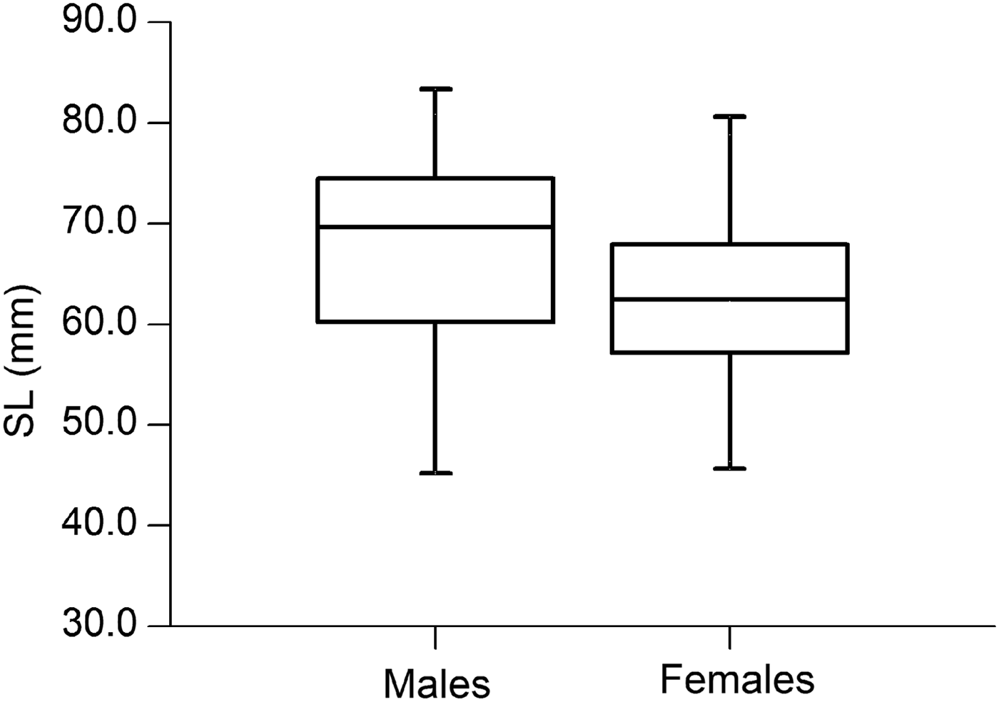
Standard length was significantly influenced by sex (F1,411 = 18.77, P < 0.001) and by the sampling month (F4,411 = 8.80, P < 0.001), but not by the interaction of these factors (F4,411 = 2.17, P = 0.072). The mean SL of mature males (66.5 mm, SE = 0.80, N = 165) was significantly larger than that of females (62.3 mm, SE = 0.50, N = 256; F1,419 = 17.32, P < 0.001) (Figure 1).
Distribution of standard length (SL) of mature individuals per sex. Each box-plot displays the middle 50% of SL, the line inside the box shows the median, and lower and upper whiskers represent the minimum and maximum SL values, respectively.

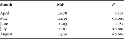
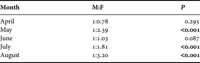
The overall males:females ratio of mature individuals (SLc B–E, N = 421) was 1:1.55, which was significantly different from the expected 1:1 ratio (P < 0.001). However, the sex-ratio fluctuated on a monthly basis, in April showing a proportion of males and females non-significantly different from parity (Table 1) and a larger proportion of females (65 %) in May–August (Table 1).
Sex-ratio of Chromis chromis captured monthly from April to August. Sex-ratios from May to August (active reproductive period) were compared to the sex-ratio of April (pre-reproductive period). The latter was compared with an expected 1:1 ratio. M, males; F, females. Significant P values are in bold.
For the whole sample, the length–weight relationship was described by the equation in the linearized form:
 $${\rm log} \;{\rm TW }= - 4.37 + 2.98 \times {\rm log} \;{\rm SL}$$
(R = 0.92, N = 9300, P < 0.001). The allometric coefficient b was close to the value of 3 which, according to Gould (Reference Gould1966), describes isometric growth.
The relationship between length and age for the whole sample was described by the von Bertalanffy's growth curve shown in Figure 2.
Von Bertalanffy growth curve. Dashed line represents the asymptotic average length, estimated by the model at 72.9 mm. Other parameter estimates: growth coefficient k = 0.567 y−1, t0 = −1.366 y.
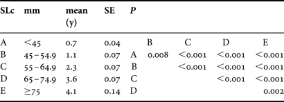
Age was significantly different among the SLc classes (F4,1007 = 227.35, P < 0.001), and older individuals were progressively larger (Table 2). The oldest individual in our sample was 7.5 yr.
Descriptive statistics of age (mean and standard error (SE)) per SL class (SLc) and P values from post-hoc pairwise comparison with Holm's correction. All P values are significant.
For mature individuals, BCI was significantly influenced by month (F4,411 = 50.97, P < 0.001) and by the interaction between month and sex (F4,411 = 8.30, P < 0.001), but not by sex alone (F1,411 = 0.87, P = 0.351).
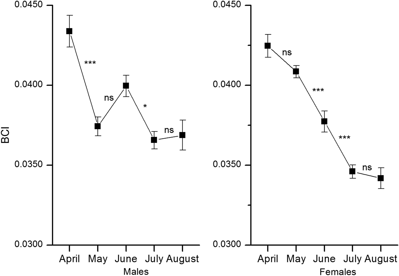
The BCI changed over months in both males and females, but in a significantly different way (F1,419 = 5.90, P = 0.016). In general, BCI decreased from April to August (Figure 3). In males, significant differences were found comparing April with May and June with July (P < 0.001 and P = 0.030, respectively, Figure 3). In females, the BCI gradually decreased showing a suggestive, but non-significant difference between April and May (P = 0.052), while a significantly lower BCI was found by comparing May with June and June with July (P < 0.001 in both cases, Figure 3).
The body condition index (BCI) monthly trend in Chromis chromis by sex. Black box, mean; whiskers, standard error.
For the whole sample, BCI was significantly influenced by month (F7,8821 = 78.4, P < 0.001), SLc (F3,8821 = 70.4, P < 0.001) and by their interaction (F21,8821 = 5.6, P < 0.001).
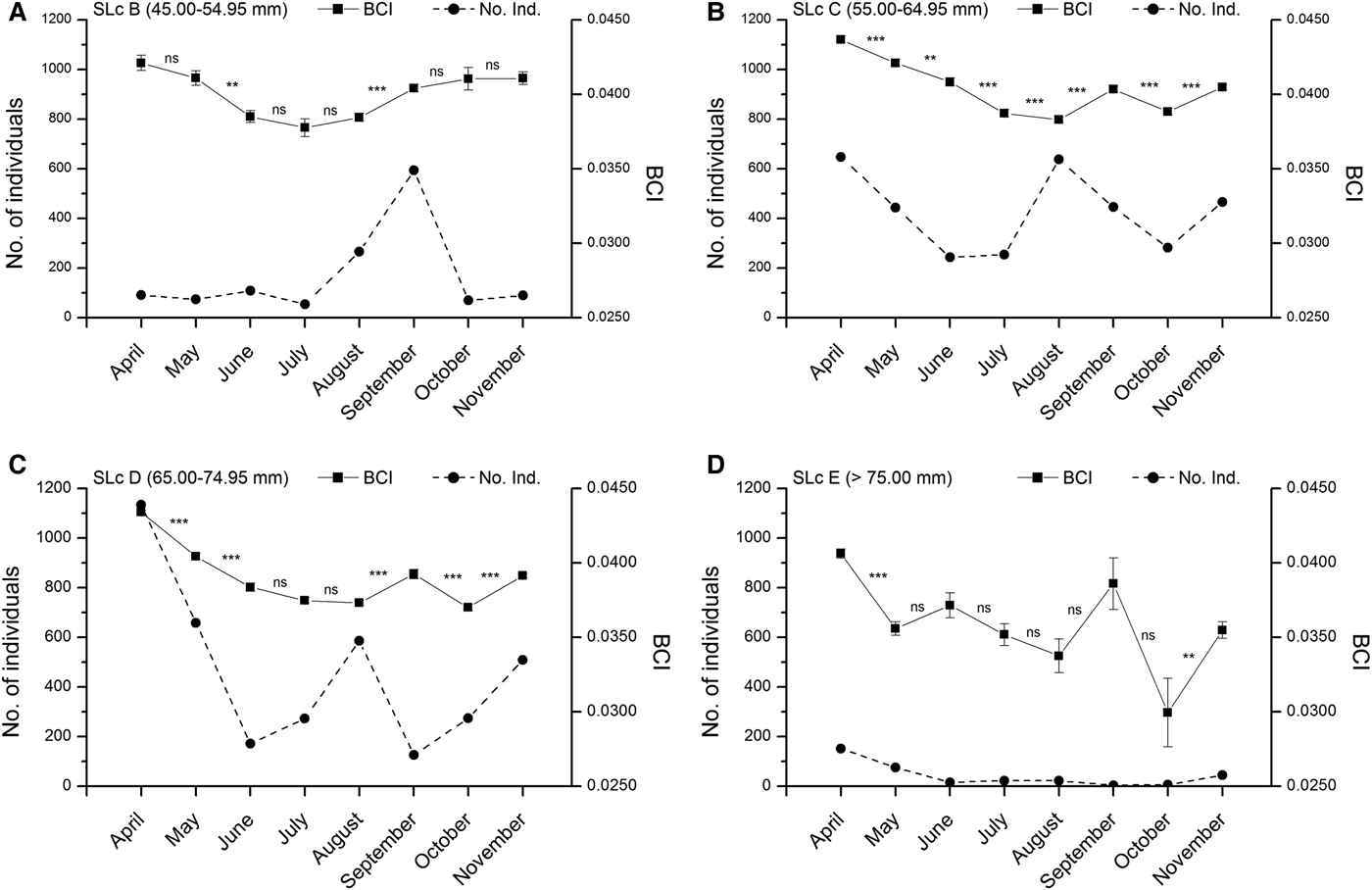
The BCI of smaller mature individuals (SLc B) showed a downward trend culminating in a negative peak in July, followed by an upward trend (Figure 4A). In larger specimens (SLc C and D) the negative trend reached its peak one month later (i.e. in August) and was followed by a fluctuation, showing a rise in September, a fall in October and another rise in November (Figure 4B–D). Specimens belonging to SLc E showed a more fluctuating trend, with three remarkable drops in May, August and October, each followed by partial recovery. In particular, the October drop culminated in the lowest negative peak recorded on all classes (mean BCI of SLc E in October: 0.0299, SE = 0.0023; Figure 4D).
Monthly captures (straight line) and body condition index (BCI) (dashed line) for standard length-classes: (A) SLc B (45–54.9 mm); (B) SLcC (55–64.9 mm); (C) SLcD (65–74.9 mm); (D) SLcE (≥75 mm). Black box, mean; whiskers, standard error.
On average, during the sampling period, individuals of SLc B, C and D were able to recover up to 90% or more of the mean BCI value observed on the first month of sampling, April (BCI in November was 97.6%, 92.6% and 90.2% of BCI observed in April for SLc B, C and D, respectively; Figure 4). The mean BCI value recorded in November on larger individuals (SLc E) was 87.2% of the mean BCI observed in April for the same class.
The number of captures per SLc showed considerable monthly variation (Figure 4). The number of individuals of SLc B remained low till July, then a positive trend began, with a remarkable peak in September followed by a steep drop in October (Figure 4A). Individuals of SLc C and D showed a more fluctuating trend, with a negative peak in June followed by an inversion of trend and a positive peak in August, and then another drop in autumn followed by a recovery. The number of individuals of SLc E remained low all through the sampling period, with mild fluctuations (Figure 4D).
DISCUSSION
Population structure
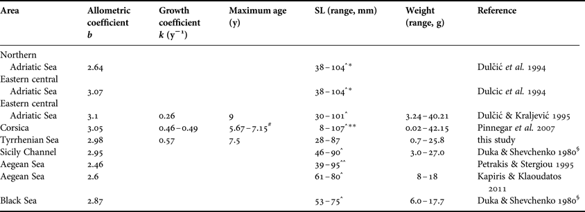
In the Mediterranean Sea, the SL of C. chromis is known to range on average from a minimum of 30 mm in the east-central Adriatic to a maximum of 107 mm in Corsican waters (recalculated from original data, Table 3). Our population from the Tyrrhenian Sea ranged from 28 to 87 mm, which fits well within known values. While the minimum length observed in our population was close to the value reported for the Adriatic Sea, the maximum length was closer to values known for the Channel of Sicily (Table 3).
Summary of allometric and morphometric values observed in Chromis chromis in the Mediterranean Sea. SL, standard length; ^ recalculated from total length; ^^ recalculated from fork length; * from length-classes, not the actual minimum and maximum values; ** not sampled by fishing; # depending on model used to estimate the age.
§Cited in Dulčić & Kraljević (Reference Dulčić and Kraljević1995).
The maximum age recorded in this study was 7.5 yr, which highlights a lower maximum age than previously observed in the Adriatic Sea (9 yr (Dulčić & Kraljević, Reference Dulčić and Kraljević1995); Table 3), but similar to that estimated by modelling a Corsican population (Pinnegar et al., Reference Pinnegar, Polunin, Videler and de Wiljes2007; Table 3). As expected for a population characterized by younger-aged, smaller individuals, the growth rate coefficient we observed in the Tyrrhenian Sea indicates an intermediate growth rate, while the Adriatic and the Corsican populations, characterized by comparatively larger individuals, were described by slower growth rates (Table 3). Fish growth depends on the energy resources allocated to somatic growth and among the main factors is the fish feeding regime (Holm et al., Reference Holm, Refstie and Bø1990; Russell et al., Reference Russell, Fish and Wootton1996; Mōllmann et al., Reference Mōllmann, Kornilovs, Fetter and Kōster2005). However, non-interactive factors such as temperature and light also play an important role (Pauly, Reference Pauly1980; Boeuf & Le Bail, Reference Boeuf and Le Bail1999). Indeed, metabolic rate in ectothermic organisms is usually higher at increasing temperatures (Clarke & Johnston, Reference Clarke and Johnston1999), which affects the growth rate (Houde, Reference Houde1989; Mooij et al., Reference Mooij, Lammens and Van Densen1994). For example, it has been proposed by Copp et al. (Reference Copp, Fox, Przybylski, Godinho and Vila-Gispert2004) that the latitudinal gradient of growth patterns in the pumpkinseed sunfish Lepomis gibbosus, an omnivorous nest guarding fish inhabiting freshwaters, may be masked by local factors such as predator pressure and competition (Copp et al., Reference Copp, Fox, Przybylski, Godinho and Vila-Gispert2004).
Relationships between length and weight of Mediterranean C. chromis have been described by several authors (Table 3), and all possible values (i.e. describing isometric, as well as positive or negative allometric relationships) have been reported. The allometric coefficient b describes fish shape, with negative values corresponding to thinner bodies and positive values to thicker bodies. Values close to those describing perfect isometric relationships (b = 3, see Gould, Reference Gould1966) have been found in populations from the Channel of Sicily and from Corsica, as well as in our samples from the Tyrrhenian Sea (Table 3). The length of our sampling period was eight months and started before the reproductive period. Although the overall length–weight relationship was described by an isometric coefficient (2.98), the value observed during the reproductive period was negative (e.g. 2.84 in July), while the one observed before reproduction was fully isometric (e.g. 2.99 in the month of April). This suggests that the overall isometric relationship was the result of a seasonal balance. Nevertheless, both negative and positive values during the reproductive season have been reported for the Adriatic Sea (Dulčić et al., Reference Dulčić, Kraljević and Cetinić1994; Dulčić & Kraljević, Reference Dulčić and Kraljević1995; see Table 3). Observed differences could be due to seasonal changes in population dynamics, and could be influenced by objective (quantity or quality of the locally available feeding resources, predation pressure, genetic factors) and subjective factors (length and timing of sampling periods).
The existence of differences among local populations (Adriatic vs Tyrrhenian, etc.), as shown by parameters such as growth and body condition coefficients, suggests that population dynamics could evolve according to oceanographic gradients both at the landscape (e.g. latitudinal or longitudinal) and at the small spatial scale, fulfilling a prerequisite for the identification of C. chromis as a promising bioindicator. Other points in favour of the use of C. chromis as a bioindicator are the species’ widespread abundance and distribution, coupled with its sedentary habits (Guidetti, Reference Guidetti2000), as well as with its ability to adapt to local environmental variability (Bracciali et al., Reference Bracciali, Campobello, Giacoma and Sarà2012).
It is worth noting here that in our population the mean SL of mature males was significantly larger than that of females (SL: 66.5 mm vs 62.3 mm, respectively). A previous study carried out in the central Adriatic did not find any difference in length (SL: 73.9 m vs 74.0 mm; Dulčić, Reference Dulčić2005), as well as in other morphometric characteristics. In contrast, a limited data set from the Aegean Sea showed greater variation in females than in males, both as concerns length and body mass (TL: 81–106 mm vs 89–99 mm and weight 8–18 g vs 12–15 g (Kapiris & Klaoudatos, Reference Kapiris and Klaoudatos2011)). It would seem, therefore, that different C. chromis populations show different sex-related morphometrics. If these were confirmed, it would be worth investigating the factors shaping such morphometric relationships (i.e. genetic and/or environmental factors).
Seasonal variation
In the Mediterranean Sea, the reproductive season of C. chromis has been reported to extend from June to September (Abel, Reference Abel1961; Grubišić, 1982, cited in Dulčić & Kraljević, Reference Dulčić and Kraljević1995; Picciulin et al., Reference Picciulin, Verginella, Spoto and Ferrero2004; Pinnegar et al., Reference Pinnegar, Polunin, Videler and de Wiljes2007), or even as starting in May in some areas of the Adriatic (Dulčić & Kraljević, Reference Dulčić and Kraljević1995). In laboratory conditions and at constant temperatures of 24–26°C, reproduction has been observed from July to September (Contini & Donato, Reference Contini and Donato1973).
In our study, BCI values and the number of individuals captured while feeding in the water column were used to estimate the length of the reproductive period. We used BCI values to describe what happened in the period before sampling. A low BCI, for example, would be expected in July, after the June spawning.
According to trends in BCI and in the number of catches, it appears that the reproductive period started in May and went on until September. Most interestingly, a close look at the separate trends observed in the four length classes (Figure 4) points to a strong size-dependent effect. Individuals with a SL ranging from 45 to 54 mm (SLc B) were characterized by a single and continuous reproductive season lasting from May to July. Larger specimens ranging from 55 to 74 mm in SL (categories SLc C and D), which constituted the bulk of our sample, showed instead a bimodal trend, with two negative peaks of BCI in August and October. This is likely to indicate the occurrence of two spawning periods, separated by a recovery in September, possibly linked to larger food availability in August (Siokou-Frangou, Reference Siokou-Frangou1996). This trend matches well with the number of individuals not engaged in reproductive activities and consequently feeding in the water column, which showed a positive peak in the month of August. Overall, the lowest BCI negative peak was recorded in October for the largest individuals (SLc E). This category underwent a more strongly fluctuating trend, with three remarkable drops, each followed by partial recovery.
As SL was age-dependent, the higher allocation of resources of larger and consequently older damselfishes is in line with the classical life-history models predicting that reproductive investment should increase with age, peaking in an act of terminal investment when there are no further opportunities for reproduction (Williams, 1966).
In multiple-spawning fish, the last spawning cycle is known to cause the depletion of the energetic reserves allocated for reproduction (Kooijman, Reference Kooijman2010; Sarà et al., Reference Sarà, Rinaldi and Montalto2014), so that larger individuals are unable to recover their original BCI values before the end of the reproductive season (i.e. BCI April vs November, post-hoc pairwise comparison test, P values: SLc C < 0.001; SLc D < 0.001; SLc E = 0.005, Figure 4B–D), in contrast to the smaller ones (i.e. SLc B, April vs September, post-hoc pairwise comparison test, P = 1.000). These findings suggest that, in spite of their high investment at the beginning of the reproductive season, our larger specimens were able to regain the metabolic energy necessary to afford further spawning, thereby probably extending their reproductive season until September. In short, the larger the size of the specimen, the better its status and the longer its reproductive season. This result might be better described by state-dependent life-history theory, which assumes that reproductive investment decisions depend on body condition, which may change as an individual grows older (McNamara & Houston, Reference McNamara and Houston1996).
Differences in habitat use between sexes have been reported for the pre-reproductive period (Aburto-Oropeza et al., Reference Aburto-Oropeza, Sala and Sánchez-Ortiz2000), with Pinnegar et al. (Reference Pinnegar, Polunin, Videler and de Wiljes2007) noting that, during the day, C. chromis males were comparatively more numerous than females on Posidonia seagrass. In our case, the sex-ratio of individuals captured in the month of April (e.g. before the reproductive season), was slightly in favour of males (M:F 1:0.78, Table 1), although the ratio was not significantly different from parity. The proportion of males in the water column decreased from May, meaning that, during the reproductive period, shoals were mainly composed of females. This reflects the damselfish reproductive behaviour, according to which males migrate to the bottom (Verginella et al., Reference Verginella, Spoto, Ciriaci and Ferrero1999; Gladstone, Reference Gladstone2007a) and remain close to their nest for about 10 days, while females go to the sea bottom only at the time of oviposition (Picciulin et al., Reference Picciulin, Verginella, Spoto and Ferrero2004). Therefore the fluctuations in sex-ratio that we observed fits well the multiple-spawning behaviour known for the species (Verginella et al., Reference Verginella, Spoto and Ferrero2000).
From a metabolic perspective, the general decrease in BCI that we observed from April to August in both sexes suggests that a greater energy demand was required during gonadic development and reproduction (Figure 3). Indeed, while females had to face costs for eggs production (Armstrong & Witthames, Reference Armstrong and Witthames2012; Bapary et al., Reference Bapary, Amin and Takemura2012), males had to sustain those related to territoriality and parental care (Gladstone, Reference Gladstone2007a). Although in both sexes BCI showed higher values before the reproductive season and lower values during the reproductive season, this decrease followed different patterns. In males, a strong decrease was observed from April to May, probably corresponding to the time of their first seasonal colonization of the bottom (Boddeke, Reference Boddeke1963; Charnov et al., Reference Charnov, Orians and Hyatt1976; Gladstone, Reference Gladstone2007a), followed by a partial recovery in June (Figure 3). In contrast, female BCI gradually decreased in spite of the possibility of having access to zooplankton by remaining in the water column, thus suggesting an additive effect of multiple ovipositions, not sufficiently counterbalanced by the energy acquired by feeding in the water column. Indeed, even if before the reproductive period the BCIs of the two sexes were close, at the end of the sampling season it was lower in females than in males (0.0280 vs 0.0320, Figure 3). These findings suggest that overall seasonal energetic investment in reproduction was higher in females than in males. It is also possible that physiological and/or behavioural differences between sexes allowed males to recover between the consecutive spawning cycles and to end the reproductive season with overall greater energetic reserves. Further studies focused on the different management of the energetic budget in C. chromis males and females could provide useful insights for supporting classical or state-dependent life-history models.
CONCLUDING REMARKS
Even though drivers are probably different between the sexes, C. chromis also shows different seasonal dynamics depending on individual size. Females might adjust their reproductive period according to mechanisms of internal regulation, such as trade-off energy allocation between body maintenance and gonadic maturation (Kooijman, Reference Kooijman2010), while males might be mainly driven by external stimuli, such as mating opportunities (Picciulin et al., Reference Picciulin, Verginella, Spoto and Ferrero2004; Gladstone, Reference Gladstone2007a). However, individuals carry on their life history activities primarily as a function of their energetic reserves (Kooijman, Reference Kooijman2010), as well as according to social organization and hierarchy (Aburto-Oropeza et al., Reference Aburto-Oropeza, Sala and Sánchez-Ortiz2000) and even individual cognition and learning processes (van Deurs et al., Reference van Deurs, Behrens, Warnar and Steffensen2011). We can say, therefore, that any observed shift in expected age/size class composition and/or BCI occurring on a local scale will be a consequence of often cryptic variations in ecological parameters such as food availability or perhaps water temperature. To implement fully adequate conservation activities, any such change should be carefully monitored, evaluated and taken into account.
ACKNOWLEDGEMENTS
We wish to thank Capitaneria di Porto di Palermo; Pietro Rizzo and Fabio Fiorentino (IAMC-CNR, Italy) for their help in otolith analysis, Gaspare Guzzo and Claudia Cavallaro (University of Palermo, Italy) for their help in laboratory and fieldwork and Emilio Balletto (University of Torino, Italy) for manuscript revision.
FINANCIAL SUPPORT
Funds were provided by DINAUTIS project by the Italian Ministry for the Environment.