I. INTRODUCTION
Composite materials are commonly designed from building blocks with contrasting material properties with the goal of combining two attractive properties in one material system. For structural applications, it is of particular interest to understand how to design composites that effectively combine the properties of stiffness and toughness. Experimental investigations have shown that many mineralized biological composites combine these two properties very well, e.g. human bone and nacre.Reference Espinosa, Rim, Barthelat and Buehler1–Reference Barthelat3 To exploit the full potential of composite systems in the context of toughness and stiffness, it is imperative to attain a fundamental understanding of the key design mechanisms governing the fracture response of composites.
Significant experimental, computational and theoretical work has been performed to explain the superior toughness of biological composite systems and many interesting mechanisms have been proposed. The more common and notable mechanisms cited include, but are not restricted to: energy dissipation and ductility through protein unfolding in the organic matrix phase,Reference Smith, Schaffer, Viani, Thompson, Frederick, Kindt, Belcher, Stucky, Morse and Hansma4,Reference Fantner, Hassenkam, Kindt, Weaver, Birkedal, Pechenik, Cutroni, Cidade, Stucky, Morse and Hansma5 frictional dissipation due to shearing of mineral-organic interfaces,Reference Gupta, Wagermaier, Zickler, Aroush, Funari, Roschger, Wagner and Fratzl6,Reference Wang, Suo, Evans, Yao and Aksay7 cooperative deformation mechanisms at a hierarchy of structural levels,Reference Gupta, Seto, Wagermaier, Zaslansky, Boesecke and Fratzl8–Reference Barthelat, Tang, Zavattieri, Li and Espinosa11 and flaw tolerance at nanoscale attained through nanoconfinement of building blocks.Reference Gao, Ji, Jager, Arzt and Fratzl12
Here we propose that far simpler interactions—linear elastic up to a brittle breaking point—can be sufficient to lay the foundations of superior toughness in two-phase stiff biocomposite structures. Inspired by biological materials we hypothesize that the stiffness ratio, in the linear elastic regime of the constituents, controls the deformation and fracture mechanism of a composite. For a range of mineralized biological composites that combine toughness and stiffness, such as nacre, bone, dentin, and enamel, the stiffness ratio between the stiff mineral phase and the softer organic phase is quite similar, despite the structures being composed of varying constituents.Reference Jackson, Vincent and Turner13–Reference Dunlop and Fratzl17 We hypothesize that purely elastic effects can induce large-scale toughening and that we can produce a wide range of composites by simply tuning the constitutive relations of the constituents. It is clear that natural composites contain a large number of structural intricacies and models thereof could be made arbitrarily complex. However, we identify the noted structural feature as a key design mechanism and use simple computational models to reflect and isolate this particular structural feature to perform an unambiguous study. The model is not intended to describe the full complexity of natural composites, but rather, it is developed to examine purely elastic effects on large-scale toughening, as outlined above.
The combination of theoretical and computational analysis of bio-composites has been very successful, and interesting models have been proposed to predict the response of layered composites such as nacre.Reference Barthelat, Dastjerdi and Rabiei18 Previous computational and theoretical studies have shown that small stiffness ratios can lead to crack tip shieldingReference Ji and Gao19 and indeed for vanishing stiffness-ratios, crack tip driving forces have been shown to disappear completely in stratified structures.Reference Fratzl, Gupta, Fischer and Kolednik20,Reference Okumura and de Gennes21 However, at a disappearing stiffness-ratio, and a finite extensible compliant phase, the failure mechanism transitions to failure by delamination, and other mechanisms are necessary to ensure structural reliable materials. Here, by adopting another bioinspired topology we aim to combine vanishing stress concentrations and structural reliability in composites with linear elastic constituents, thereby proposing novel design mechanisms for superior tough composites. We further hypothesize that we can assemble a stiff composite with superior toughness at a “minimal cost” by combining two building blocks, whose fully elastic constitutive laws are intimately correlated, exhibiting the identical inferior toughness. We stress that by endowing such simple constitutive relations for the constituents of our model composites, we ensure that stress delocalization, load redistribution, and other observed toughening mechanisms can be attributed solely to the topological arrangement of the constituents and more importantly; their stiffness mismatch.
II. MATERIALS AND METHODS
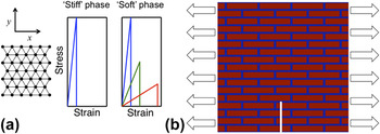
Here we focus on model materials that are meant to represent general materials and composite systems. We utilize a triangular spring-bead lattice where the interactions between beads are governed by springs following a linear-Hookean force extension law derived from a harmonic potential. Figure 1(a) shows the material representation. Here, we allow springs, representing the bonds between the beads, to break if they extend beyond some critical length, r c. This represents the initiation or growth of a crack and the system will fail if a crack, the breaking of bonds, percolates through the network. This class of model received much attention in the late 1980’s when used extensively to study the influence of randomness and disorder on the fracture behavior of various materials.Reference Beale and Srolovitz22–Reference Sahimi and Goddard24 Further, in the context of fracture mechanics, triangular lattice spring bead models were shown to reproduce numerical continuum mechanical solutions for stress intensity factors in various systems.Reference Curtin and Scher25 Here, we allow springs, the bonds between the beads, to break if they extend beyond some critical length, r c. This represents the initiation or growth of a crack and the system will fail if a crack, the breaking of bonds, percolates through the network.
(a) Triangular lattice spring-bead material representation to describe a coarse-grained model of the material. All lines are of identical length. We present the constitutive relations for stiff phase as well as three example constitutive relations for the soft phase, representing the first three combinations of elastic properties listed in Table I. The area under all four curves drawn is identical. (b) Brick and mortar composite topology considered here. Platelets are drawn in red while the matrix phase is represented with blue. The notch and mode I loading conditions used here are also represented.

The intuitive representation of cracks, as the breaking of bonds, combined with the documented agreement with and good representation of continuum fracture mechanics concepts provides us with the confidence to use this model for the study of the fracture mechanical behavior of bio-inspired composites. We model the respective phases of our composite as homogeneous, and thus our system is represented by an ordered heterogeneity. Similarly to the representations in Refs. Reference Beale and Srolovitz22–Reference Sahimi and Goddard24, our beads represent a group of smaller particles/molecules, however in our system we choose these beads to be large enough to neglect intrinsic disordered heterogeneity. Heterogeneity commonly arises at the nanoscale in biological systemsReference Fratzl and Weinkamer10,Reference Tai, Dao, Suresh, Palazoglu and Ortiz26–Reference Gupta, Stachewicz, Wagermaier, Roschger, Wagner and Fratzl28 and our model presented here represents a mesoscale system.
As we wish to focus our attention on the interaction between the different phases in a composite we study a single topological ordering of the respective phases. We use the brick and mortar like structure of stiffer platelets dispersed in a soft matrix, portrayed in Fig. 1(b), which is used in several natural systems, such as bone and nacre.Reference Landis29,Reference Menig, Meyers, Meyers and Vecchio30 We deal with perfectly elastic materials and further keep the constitutive relation of the platelets constant. The platelets will henceforth often be referred to as the stiff phase, even though they may follow the same constitutive relation as the matrix phase, which correspondingly will also be referred to as the softer phase. The softer phase comprises approximately 20% of the entire volume of the structure. We choose this volume fraction as it allows us to model minimal volume fraction of the matrix phase at a low computational cost. Restricting the volume fraction of the more compliant phase is critical as a fundamental goal of this study is to create a composite combining appreciable stiffness with toughness.
We aim to show that purely elastic materials with appropriate elastic constants can be combined in a generic composite topology, such as the brick and mortar geometry, to create tough composites. Although an energy dissipating matrix phase is indeed suited for the assembly of tough composites, we hypothesize that it is not necessary and we show this by using linear elastic perfectly brittle constitutive relations of the stiff and soft phase with identical toughness modulus. The force extension law of our springs is parameterized with a spring constant k and a critical extension r c. By use of the Cauchy-Born rule and geometrical considerations the spring stiffness and critical spring extension are readily translated to an equivalent Young’s modulus, E, and failure strain, εc.Reference Buehler31 It is easily validated that
 $${{r_{{\rm{c}},{\rm{soft}}} } \over {r_{{\rm{c}},{\rm{stiff}}} }} = {{{\rm{\varepsilon }}_{{\rm{c,soft}}} } \over {{\rm{\varepsilon }}_{{\rm{c,stiff}}} }}\quad {\rm{and}}\quad {{k_{{\rm{soft}}} } \over {k_{{\rm{stiff}}} }} = {{E_{{\rm{soft}}} } \over {E_{{\rm{stiff}}} }}\quad.$$
We introduce the parameter ρ to represent the stiffness ratio,
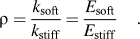 $${\rm{\rho }} = {{k_{{\rm{soft}}} } \over {k_{{\rm{stiff}}} }} = {{E_{{\rm{soft}}} } \over {E_{{\rm{stiff}}} }}\quad.$$
Enforcing the constraint that any two phases have the same toughness modulus leads to a scaling law relating the stiffness ratio and failure strains:
 $$r_{{\rm{c,}}{\rm{soft}}} = r_{{\rm{c}},{\rm{stiff}}} \sqrt {{1 \over {\rm{\rho }}}} ,\,{\rm{\varepsilon }}_{{\rm{c}},{\rm{soft}}} = {\rm{\varepsilon }}_{{\rm{c,}}{\rm{stiff}}} \sqrt {{1 \over {\rm{\rho }}}}\quad .$$
The two equalities in Eq. (3) are equivalent.
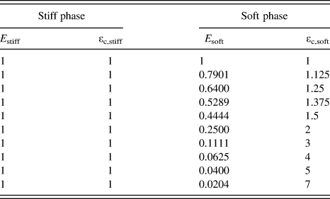
Figure 1(a) further shows the constitutive relation of the stiffer phase as well as three examples of constitutive relations of the softer phase. Table I presents an overview of all variables listed with their respective definitions, and Table II summarizes the ensemble of constitutive laws used in this study. We do not model specific natural systems nor any particular material, and thus we find it convenient to express our parameters and results in nondimensional units.
Overview of variables, dimensions and their definitions. Dimensions are given in terms of the base dimensions M, L, T.

Elastic constants for the stiff (platelets) and soft phase (matrix) of the composite. Constants are expressed in normalized units,  $E \cdot {\rm{\varepsilon }}_{\rm{c}}^{\rm{2}} = {\rm{const}}$.
Several interesting studies on mineralized structures attribute toughening mechanisms to interfacial sliding effects occurring at the interface of soft organics and the brittle mineral crystals.Reference Wang and Gupta32 Moreover, other studies have presented rigorous models of the interfacial mechanisms in composites and studied these in detail.Reference Argatov33 In the models presented here we assume a perfect bonding between the two phases, the interface is as strong as the weakest phase. Although, in many real composite systems this assumption may not be appropriate, it serves an important purpose in this study. Namely, we exclude any interfacial effects and truly only investigate the effect on the macroscale mechanical properties of varying constitutive relations of the matrix phase.
As indicated in Fig. 1(b) our samples can be regarded as single edged notched tensile specimens. The crack extends to a tenth of the specimens length in the y-direction and maintains the same length for all tested samples. We implement periodic boundary conditions in the x-direction to prevent boundary effects at the location of load application. Further, we simulate quasi-static loading with incremental displacement boundary conditions and consecutive energy minimizations with the conjugate gradient technique in the LAMMPS package. We test each system four times, each time with different displacement increments, to ensure that the energy minimization works properly, i.e., does not cause the system to diverge from a global minimum, for a given displacement increment. The four strain increments used are 0.42, 0.84, 1.69, and 3.38 × 10⁻⁵.
We record the positions of the beads at each displacement step thereby allowing us to track stress and strain as the samples are stretched. Stress is expressed through the virial descriptionReference Tsai34 and we study local strains by means of a local atomistic deformation gradient.Reference Zimmerman, Bammann and Gao35 The computed local stresses and strains are evaluated by visualization of stress and strain fields plotted in MATLAB. Stress and strain fields represent an important analysis tool in this study as they provide insight into the modes of deformation and failure of the materials.
III. RESULTS
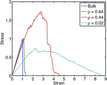
The range of composite behaviors achieved by tuning the interactions between the two phases is visualized in Fig. 2. We present the stress versus strain response of four representative samples; the stiff bulk system, included as a baseline, and three composite structures with stiffness ratios, ρ = 0.64, 0.44, and 0.02. The bulk baseline system, with the same constitutive relation for both phases, behaves perfectly linear elastic and exhibits brittle failure, as expected. The three composite systems exhibit three fundamentally different behaviors.
Stress-strain responses for the bulk system and three composite structures, ρ = 0.64, 0.44, and 0.02 (recall that ρ = E soft/E stiff). The strain and the stress are normalized by the maximum strain and stress of the brittle bulk system. Graphs indicate the rapid change in composite behavior as the stiffness ratio is varied.

The first thereof, indicated in green, is a system that behaves very similarly to the bulk system; we record a negligible increase in peak stress and a virtually unchanged Young’s modulus. The second composite system in Fig. 2, indicated in red, reaches a peak stress almost twice as large as the baseline system while compromising only a fraction of the bulk stiffness. Finally, the third presented composite, indicated in cyan, is the most compliant of the three and exhibits a ductile response with a gradual stable failure. The simple tuning of the constitutive law of the matrix phase, constituting only 20% of the sample volume, has had a large influence on the composite structural response and given rise to three fundamentally different composite behaviors. We further notice that the two latter composites notably prolong their prepeak elastic response. This indicates that we have succeeded in reducing stress concentrations while retaining structural reliability with very simple building blocks, akin to mineralized biocomposites. Indeed, these results indicate that the composite design has induced essential deformation mechanisms contributing to a more efficient load distribution. While it is a well known fact that composites can attain mechanical properties superior to their constituents, it is of particular interest that the composites studied here exhibit these performances with such simple interactions of the constituents. Indeed, this indicates that the stiffness ratio ρ plays an essential role in the mechanical performance of the system, as hypothesized. In an effort to gain a more fundamental understanding of the mechanical principles governing these composite responses we now analyze stress and strain fields of the samples.
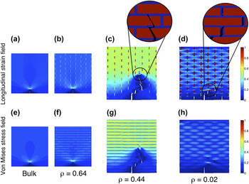
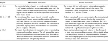
Figure 3 shows strain and stress field plots, drawn at the instant the structures endure their peak loading, for the three composite systems as well as the stiff bulk system. We clearly see from Figs. 3(b) and 3(f) that the ρ = 0.64 system behaves very similarly to the perfectly brittle bulk system shown in Figs. 3(a) and 3(e). This stiffness ratio proves insufficient to significantly redistribute strain and stress from the crack-tip, and the large localization of stress and strain at the tip of the flaw is maintained. However, once the stiffness ratio drops below 0.5 to ρ = 0.44 [Figs. 3(c) and 3(g)] a fundamental change in deformation mechanisms occurs. For the current geometrical configuration, the mismatch in stiffness is sufficient to accommodate a delocalization of strains from the “critical” flaw to the softer matrix. Thereby, strains are spread throughout the system, and the entire composite is incorporated in the strain and stress transfer leading to a more beneficial structural response.
Longitudinal strain fields and Von Mises stress fields for the bulk system, (a) and (e); the composite structures with stiffness ratios ρ = 0.64, (b) and (f); ρ = 0.44, (c) and (g); and ρ = 0.02, (d) and (h). The longitudinal strain field plots clearly show the softer phase absorbing an increasing portion of the strain as the stiffness-ratio decreases. This affect is accompanied by a delocalization of stress and strain from the crack tip and increased stress and strain in regions far from the crack tip. Panels (c) and (g) clearly exhibit the superior performance of the ρ = 0.44 composite structures. Insets for panels (c) and (d) indicate a transition in the fracture mechanism.

Taking the stiffness mismatch one step further we obtain the responses shown in Figs. 3(d) and 3(h), and we record a new shift in the composite deformation mechanism. Now the compliance of the matrix phase is so large that the matrix phase adsorbs a large share of the deformation of the entire structure and the stress level in the stiffer platelets is significantly reduced. The overall structural response is controlled by the matrix phase, leading to a more compliant load-deformation behavior and allowing the system to reach larger levels of strain.
Moreover, the insets in Fig. 3 show that the fracture mechanism also changes as the stiffness ratio decreases from ρ = 0.44 to ρ = 0.02. Whereas the fracture propagates through both the platelet and matrix phase for the composite with ρ = 0.44, it has become energetically more favorable for the fracture to move solely through the matrix phase in the softer system. The fracture mechanism has transitioned to a platelet pullout mechanism akin to biological brick and mortar systems.Reference Song, Soh and Bai36 This mechanism is likely a direct result of the large stiffness mismatch in the composite structure and the large crack deflection angle may lead to significant additional toughening. Moreover, the large deflection angle leads to an increased pathlength of the crack, which also results in additional robustness of the system. In a natural biological material such as nacre, with a stiffness ratio similar to this composite system, platelet pullout is a favorable failure mechanism as it activates additional toughening mechanisms such as frictional dissipation originating from interfacial sliding, breaking of nanoasperite bridges, and protein unfolding in the organic matrix. The ability of our composite system to replicate this fracture mechanism leads us to believe that we have indeed identified a key composite design mechanism. Furthermore, the result indicates that the large stiffness mismatches displayed in natural composites plays an important role in facilitating platelet pullout. We further note that in our composite system the softer phase does not just act as an isolator shielding the platelets from load concentrations; on the contrary, it serves to transmit significant stresses and strains. This is a key factor contributing to the reliability of this structural system; even regions below the crack tip still have significant contributions to the overall mechanical response.
There is no doubt that the strength of the matrix phase plays an important role for the fracture mechanisms of the samples. One could argue that the lower stiffness ratio composites exhibit distributed failure by design, as their matrix phase is indeed weaker. However, an analysis of Figs. 2 and 3 shows that it is the elastic properties of the respective phases that control the fundamental shift in deformation mechanism observed. Load is distributed throughout the composite far before the matrix phase starts failing. Although the representation of the matrix phase is already very conservative in terms of mechanical properties (typically biological composites have highly extensible organic matrix phases), there is no reason why composites with weaker and less extensible matrices would not exhibit these same properties. Finally, it follows directly by the observation that the composites exhibit the delocalized stress and strain fields in the prepeak regime that the same deformation mechanisms would persist with a stronger matrix. By the discussion given above, we therefore argue that the observed delocalization of stress and strain is indeed independent of the matrix strength.
To compare the fracture properties of the composites we analyze their toughness modulus, T. The toughness modulus is defined as the area under a stress-strain curve and can thus be interpreted as the maximum strain energy density attained by the composite. This energy should not be mistaken for the dissipated energy in the spring bead network. Nonetheless, the measure expresses an important fracture resistance metric as it describes the external work required to fracture the composite. Fracture in biological materials is typically not well described by linear elastic fracture mechanics, and thus the toughness modulus is a suitable metric of fracture resistanceReference Mayer37 (rather than use methods such as the J-integralReference Rice38).
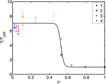
In Fig. 4, we plot the normalized toughness modulus T/T stiff versus stiffness ratio ρ for all four tensile tests of the nine different composite systems along with the benchmark results for the bulk system. As indicated, the toughness moduli are normalized by the toughness modulus of the flawed stiff bulk system. The legend identifies points on the graph with the different displacement increments used in the respective simulations, one through four representing 0.42 through 3.38 × 10⁻⁵. We see that there is no consistent trend associated with the decrease in displacement increment and conclude that our results reliably represent the behavior of our model system subjected to quasi-static displacement induced loading.
Normalized toughness modulus T/Tstiff plotted versus stiffness-ratio ρ for all four tests on the ten specimens. The legend identifies the markers indicating the results for the simulations with the various displacement increments, 1 through 4 indicating displacement increments of 0.42 through 3.38 × 10⁻⁵. The fitted curve is a sigmoid function described by f(ρ) = 1 + 6exp (−63ρ + 33)/(1 + exp(−63ρ + 33)). The parameters for this fit were found by minimizing the residual squared error to the data points and adding a nonzero regularization term. We stress that although the fit indicates two separate regimes of fracture mechanical properties of the composites; we indeed observe three different regimes of deformation and fracture mechanisms that give rise to these properties, this is highlighted in Table III.

The plot nicely represents the consequences of the deformation mechanisms we observed in Fig. 3. The first few composite systems with ρ > 0.6 notice barely any change in toughness modulus with varying stiffness ratio, while for 0.4 < ρ < 0.6 we see a rapid, almost 8-fold increase of the toughness modulus. Previous experimental investigations of natural composite structures have also revealed significantly superior fracture resistances over the bulk constituents.Reference Smith, Schaffer, Viani, Thompson, Frederick, Kindt, Belcher, Stucky, Morse and Hansma4 However, to the best of the authors’ knowledge, such a significant improvement in fracture mechanical characteristics has never before been attributed to as a simple mechanism as proposed here. This large sudden transition supports the view of a fundamental change in the deformation mechanism of the composite, as was suggested above. The interesting point here that we wish to underline is that this first shift in mechanical behavior, from traditional brittle bulk behavior to strong and tough composite behavior, occurs with such a small perturbation in the constitutive law of the matrix phase. The dramatic shift is made possible with a 30% decrease in stiffness accompanied by a 20% increase in failure strain. We see from Fig. 4 that further decreases in ρ, accompanied by increases in εc, do not have as large an influence on the toughness modulus. Revisiting the discussion given in connection with Fig. 3, it becomes clear that the key inter-constituent interaction that facilitates increases in toughness modulus of the flawed composite is the cooperative deformation that alleviates the stress localization at the crack tip.
Figure 4 displays a sigmoidal function fit to the toughness data, we can motivate this functional form of the toughness evolution by analyzing limit cases in our model. In the limit as the stiffness ratio ρ → 1, the composite behaves entirely as a brittle bulk material and the system achieves its minimum toughness modulus, the toughness is bounded from below. Further, as the respective composite phases have constant fracture energy the toughness modulus of the composite system must also have an upper bound as ρ → 0. Moreover, as the composite transitions from enduring a stress field localized at the crack tip to a delocalized stress field, a sudden transition in toughness modulus is expected. Thereby, the functional form of the fit in Fig. 4 is motivated and what remains is arguing for the point of inflection, the critical stiffness ratio. For composites with a laminated geometry at the crack tip the stress concentration at the tip of the crack is predicted to vanish as the stiffness ratio between the compliant and stiff phase decreases.Reference Fratzl, Gupta, Fischer and Kolednik20,Reference Okumura and de Gennes21 In Ref. Reference Fratzl, Gupta, Fischer and Kolednik20 the critical stiffness ratio is given as a function of the volume ratio of the softer phase, for a volume fraction of 0.2 the critical stiffness ratio is ∼0.25. In our system, the brick and mortar structure will serve to alleviate the stress concentration at a higher stiffness ratio as the strain is given a continuous path through the matrix phase.Reference Dimas and Buehler39 We can thus motivate the transition occurring at ρ > 0.25 and in the case studied here it occurs at ρ ≈ 0.5 as seen in Fig. 4. This transition point should not be interpreted as a general critical stiffness ratio as it is likely sensitive to specific system configuration. We expect the topological arrangement of the composite to be the main variable controlling this critical stiffness ratio. Moreover, in the space of bone-like geometries, the aspect ratio of the platelets likely also influences the transition. The key point to be noted here is that the transition occurs, and that it does so at a feasible stiffness ratio.
To estimate the gained toughness modulus by tuning constitutive laws of the composite constituents we again gain insight by analyzing the limiting case. As the stress concentration decreases, the deformation delocalizes completely and strain distributes throughout the entire structure. As the stiffness ratio decreases further, strain concentrates in the matrix phase, and at the asymptotic limit of a vanishing stiffness ratio the deformation of the entire structure will be completely absorbed by the softer phase. The energy required to fracture the softer matrix phase will thus account for the entire toughness modulus of the system. By design, all constituents have the same toughness modulus and we can evaluate the energy required to fracture the compliant matrix, as ρ → 0, by investigating the theoretical limit of the toughness modulus for the homogeneous system. This theoretical limit is readily evaluated by analyzing the behavior of a perfectly homogeneous defect free system. As we show in the Supporting Information, this system fails at a stress approximately five and a half times larger than the flawed bulk system. It follows that
 $$G_{{\rm{th}}} = {1 \over 2}{{{\rm{\sigma }}_{{\rm{th}}}^2 } \over E} \approx {1 \over 2}{{\left( {5.5{\rm{\sigma }}_{{\rm{br}}} } \right)^2 } \over E} \approx 30G_{{\rm{br}}} \quad,$$
where the subscripts “th” denotes theoretical, and “br” brittle, respectively. As the soft phase constitutes 20% of the volume and has the same fracture energy as the stiff phase by construction, we can estimate the gained toughness in the limiting case as,
 $$G_{{\rm{lim}}} \approx 0.2G_{{\rm{th}}} = 6G_{{\rm{br}}} \quad.$$
In the intermediate case the load and deformation will be shared by the stiff and compliant phase and thus we expect the gain in toughness to exceed this limiting value G lim. In agreement with the prediction by this model the composite systems with smaller stiffness ratio ρ exhibit approximately a 7-fold increase in toughness modulus over the brittle system.
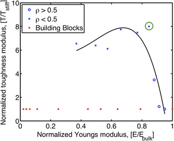
We now return to the original question posed in this paper, the question of whether we can create a composite whose building blocks exhibit only the simplest interactions that combines the properties of superior stiffness and superior toughness. To this end, we plot an Ashby plot of normalized Young’s modulus and normalized toughness modulus, Fig. 5. The relevant mechanical properties of all composites and constituents are indicated in the figure, with the color red corresponding to constituents and the color blue representing composites. To separate the tough composite from the brittle, we use different markers for composites with ρ > 0.5 and ρ < 0.5. We see that all composites with ρ < 0.5 clearly outperform their constituent materials in terms of the toughness modulus. Furthermore, a subset of our composites reach superior toughness at significant stiffness, with the toughest system retaining over 80% of the stiffness of the stiffest constituent.
Ashby plot of normalized toughness modulus versus normalized Young’s modulus. Stiffness’ are normalized versus the stiffness of the bulk system and toughness’ are normalized versus the toughness of the bulk system. Markers for composite systems with stiffness ratios ρ > 0.5 are drawn with blue circles while those for systems with ρ < 0.5 are drawn with blue crosses. The modulus-toughness combinations of the building blocks are indicated with red stars (same for all cases, by design). The superior toughness of the composite systems with respect to the individual blocks is clearly exhibited. We also see the impressive performance of the stiffest ρ < 0.5 system, circled in green, with an 8-fold increase in toughness accompanied with a stiffness of over 80% of the stiff bulk system. The fitted curve is a fifth-degree polynomial fitted by minimizing residual squared error, again with a nonzero regularization term. The curve clearly indicates that our composite structures span the Ashby area in a similar fashion as biological composites.Reference Espinosa, Rim, Barthelat and Buehler1Figure 3 exhibits the deformation mechanisms underlying the various mechanical performances indicated here. Again, we point out that although an important transition in mechanical properties occurs across ρ = 0.5, there are indeed three different regimes of deformation and fracture mechanisms that give rise to the observed mechanical responses, this is highlighted in Table III.

Finally we see that the way in which we tune the interactions between the two composite phases produces a set of composites that span the Ashby area in a similar way to biological composites, as both sets of these data points are best summarized by a concave trend line.Reference Espinosa, Rim, Barthelat and Buehler1 This observation further supports the hypothesis driving this study that the fundamental interactions in biological composites that control their superior mechanical properties are in fact governed by the stiffness ratio between the two phases.
It was previously established that stiffness ratios could be tuned to make stress concentrations vanish.Reference Fratzl, Gupta, Fischer and Kolednik20,Reference Okumura and de Gennes21 Here we have shown that by tuning constitutive laws one can further make structurally reliable systems with superior toughness. In systems where a softer matrix phase is included to alleviate stress concentrations it is clear that this matrix phase must be able to store a certain level of deformation energy to effectively redistribute loading before failing. Here we have shown that a compliant matrix in a brick-and-mortar structure can induce a significant toughening effect in a composite even though its fracture energy is limited to that of the stiff and brittle platelet phase. In this light we can view our composite structures as minimal cost structures and in mineralized biological structures where there are many more toughening mechanisms, structures can achieve yet greater toughness values.
IV. CONCLUSION
By using a simple mesoscale bead model implemented in a molecular mechanics framework we investigated the mechanics of bioinspired composite materials with a brick and mortar topology. By tuning the constitutive law of the matrix phase, we investigated fundamental mechanical interactions between the composite constituents governing system stiffness and fracture resistance with the aim of elucidating simple design mechanisms for the design of structurally robust composites. Our studies showed that the specific elastic behavior of the matrix phase controls the response of the composite and with small perturbations in the elastic behavior of this phase we achieved dramatic shifts in deformation and fracture mechanisms (as summarized in Table III). We further showed that by tuning these simple elastic interactions we could attain structures combining significant stiffness with superior toughness as well as create composites reproducing fracture mechanisms observed in mineralized biological materials. Moreover, we produced a range of composite behaviors filling an Ashby area (of stiffness and toughness) in a similar fashion as biological structures. Our results lead us to conclude that the elastic interactions we elucidate here are indeed fundamental design mechanisms in nature and with the view toward optimizing composite performance, these basic interactions may play an important role in a range of engineering applications.
Summary of key mechanisms induced by changes to the constitutive laws. We distinguish between three regimes; ρ > 0.6, 0.3 ≤ ρ < 0.5, and ρ < 0.3. The regime 0.5 ≤ ρ < 0.6 is as indicated in Fig. 4 a transition regime and is therefore not discussed here.

ACKNOWLEDGMENT
We acknowledge funding from the Army Research Office (W911NF-10-1-0127).