The financial crisis of 2008/09 and the difficulties in escaping from recession since the crisis have reawakened interest in Keynesian economic policies. This suggests that the time is right for a reappraisal of the British experience in the 1930s. This is a period with considerable relevance for today, in particular because after 1932 nominal interest rates were very low both during an initial phase of fiscal consolidation and a later one of rearmament financed partly by borrowing. More generally, much of the interwar period saw considerable slack in the British economy. The size of the fiscal multiplier in such conditions is of obvious interest to today's policymakers, just as it has been to economic historians working on the macroeconomics of interwar Britain.
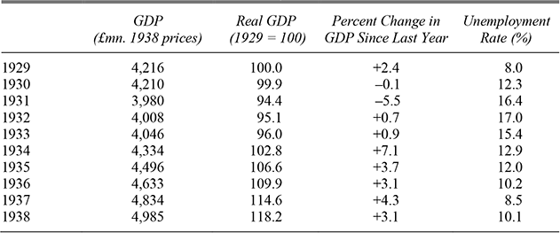
The British experience of downturn and recovery is reported in Table 1. A fall in GDP, which was very modest compared with the United States, was followed by a strong recovery in the years after 1933. Before 1935, insofar as this recovery was the result of policy, it had to come from monetary stimulus. Fiscal policy only began to play a role after 1935 when rearmament provided a de facto Keynesian stimulus.
REAL GDP, ANNUAL GROWTH RATES, AND UNEMPLOYMENT IN THE UNITED KINGDOM, 1929–1938

Sources:
Real GDP at factor cost: Feinstein (Reference Feinstein1972, Table 5). Unemployment: Boyer and Hatton (Reference Boyer and Hatton2002).
It has been a widely held belief among British economic historians that rearmament delivered a powerful stimulus in the late 1930s (Robertson Reference Robertson1983, p. 280). In taking this position, they echo the comment of The Economist that “Britain's rearmament program is the greatest public works program ever devised in time of formal peace.” (The Economist, April 22, 1939, p. 184.) A paper by Mark Thomas is the only serious attempt to quantify the impact of rearmament on economic activity (Thomas Reference Thomas1983). His method was based on an input-output table and a social accounting matrix and he found that the multiplier was 1.64 in 1935 and 1.60 in 1938. This generated an estimate that rearmament produced over a million jobs by 1938 by which time the increase of £204 million in defense expenditure since 1934 would have raised GDP by £326 million or 6.5 percent. As Roger Middleton has noted in a recent literature survey, Thomas's results have been much cited and provide “a quantitative demonstration that at least military Keynesianism worked” (Middleton Reference Middleton2011, p. 14).
Thomas's finding that the government-expenditure multiplier was about 1.6 is within the range of 1.25 to 1.75 thought plausible by Timothy Hatton in an influential review of estimates made in the 1980s which still comprise almost all the literature available today (Hatton Reference Hatton, Glynn and Booth1987). Even so, this estimate may not be reliable since it assumes away any crowding out and may therefore be too large leading to an exaggeration of the impact of rearmament. Much of the historiography focuses on the possible impact of public expenditure proposals to reduce unemployment made by John Maynard Keynes and Hubert Henderson. These proposals were taken up by the Liberal Party under David Lloyd George at the 1929 general election. T. J. Thomas estimated the government-expenditure multiplier to be 0.98 in the short-run and 1.44 in the long-run using a simulation of a Keynesian macro-econometric model. Stephen Broadberry's estimation of an IS-LM model gave a value of 1.22 for the fiscal multiplier (Thomas 1981; Broadberry Reference Broadberry1986).
More recently, Nicholas Dimsdale and Nicholas Horsewood incorporated aggregate supply with a high degree of nominal inertia as well as aggregate demand into a macroeconometric model for the interwar period. They conclude that the short-run multiplier was about 1.5 and the long run as much as 2.5 (Dimsdale and Horsewood Reference Dimsdale and Horsewood1995). All of these authors explicitly or implicitly conclude that the impact of government expenditure on employment would have been considerably lower than claimed by Keynes and Henderson. Low enough that Lloyd George “could not have done it.”Footnote 1 The methods employed in these papers to obtain estimates of the multiplier are open to challenge and are not those which would be used by macroeconomists today. The models they rely upon basically embody Keynesian ideas in their specification with a traditional consumption function and may not adequately reflect crowding out, with the implication that the estimated multipliers are too large. For example, models in either the modern neoclassical or new Keynesian traditions which embody optimizing behavior by forward-looking households typically expect consumer expenditure to fall rather than increase in response to an increase in government expenditure—in other words: the multiplier may be less than 1.Footnote 2 If these models of a more recent vintage were applicable to the 1930s, then the strong likelihood is that the conventional wisdom that rearmament had a big impact on GDP would be incorrect. This suggests that a fresh look at the size of the multiplier in 1930s' Britain using modern techniques is desirable.
Given that theoretical predictions are model-dependent, it is important to let the data speak and, since the seminal paper by Olivier Blanchard and Roberto Perotti, vector autoregression (VAR) techniques have often been used to estimate multipliers from quarterly macroeconomic time series, although many economists prefer to base their ideas of the value of the multiplier on the results of calibrations of dynamic stochastic general equilibrium (DSGE) models, where an interesting aspect is how far these may vary according to the state of the economy (Blanchard and Perotti Reference Blanchard and Perotti2002).Footnote 3 The big problem in estimating multipliers using VARs is the validity of the identification assumptions that are made, in particular whether government expenditure can be treated as exogenous and unanticipated.Footnote 4 It is fair to say that the use of these techniques has produced quite a wide range of estimates of the size of the government-expenditure multiplier (ΔY/ΔG) for the postwar American economy, with a recent authoritative survey concluding that it probably lies between 0.8 and 1.5.Footnote 5
Building a convincing DSGE model for the interwar British economy would be an ambitious undertaking. However, it is now possible to revisit the question of the size of the fiscal multiplier using time-series econometrics rather than relying on a traditional macroeconomic model, as has been the practice hitherto, thanks to the development of a quarterly series for real GDP for the interwar U.K. economy by James Mitchell, Solomos Solomou, and Martin Weale (Reference Mitchell, Solomou and Weale2012).Footnote 6 This is our focus. In undertaking this task, we make use of Valerie Ramey's approach to resolving the endogeneity of government expenditure using announcements of new expenditures (Ramey Reference Ramey2011b). She argues for the use of changes in the present value of expected future defense spending and both she and Robert Barro and Charles Redlick have implemented this approach in recent papers (Ibid.; Barro and Redlick Reference Barro and Redlick2011). Their estimates of the multiplier vary a bit according to the sample period used but for the postwar era both papers suggest a range of 0.6 to 0.8. We construct a defense-news variable from contemporary sources and develop a similar analysis to estimate ΔY/ΔG for interwar Britain. We use the results to provide a reappraisal of the claims in the historiography relating to the possible impact on real GDP both of the hypothetical Lloyd George fiscal stimulus, or “the Keynesian solution,” and of the actual rearmament program.
DEFENSE NEWS
The aim of “Defense News” is to reflect changes to planned government defense expenditure previously unanticipated by the public. More precisely, the aim is to chronicle changes in the information set available to an informed member of the public and calculate their implications for the expected present value of future defense expenditure. This variable can be thought of as capturing exogenous shocks to a key component of government spending.
The series for changes in the expected present value of government expenditure on defense for the United Kingdom in the interwar period has been constructed using a similar method to that employed by Ramey who mainly used information from Business Week (Ramey Reference Ramey2009).Footnote 7 Our key source is The Economist magazine, which was published weekly through the interwar period. This source gives details of defense estimates, which were usually published in government papers in February and March each year, but there were sometimes also supplementary estimates. The Economist gave a detailed yearly account of actual spending at the time of the annual budget in April. It also published quarterly running totals at the beginning of January, April, July, and October each year, and from time to time provided commentary on the prospects for defense spending in editorials and in featured news items.
In order to construct the series for “Defense News,” we examined every issue of The Economist from 1919 through 1938 and compiled a complete log of all entries relating to defense expenditure. The relevant material includes reports of defense estimates, announcements of policy changes with possible spending implications, special reports such as those on air force and naval expenditure in February 1936, commentaries on the credibility of government estimates and announcements, and predictions of future developments. Most of these items lend themselves to straightforward quantification. Wherever The Economist provides a clear indication as to its expectation of the likely course of future defense expenditure, we have accepted that as part of the public's information set. The volume of material varies considerably over the years; for example, there are many entries for the late 1930s but few for the late 1920s. Statistical information obtained from The Economist has been cross-checked against the detailed descriptions of British budgets provided by Bernard Mallet and Oswald George and by Basil Sabine (Mallet and George Reference Mallet and Oswald George1929, Reference Mallet and Oswald George1933; Sabine Reference Sabine1970).
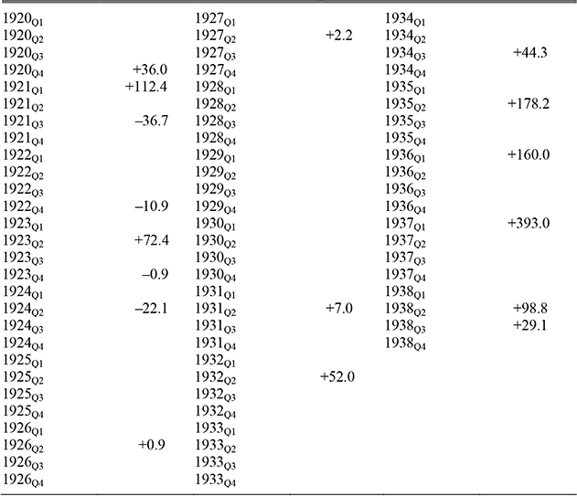
Using the log, we made an estimate of the present discounted value of defense expenditure for 1920 quarter 1 and then updated it each quarter until 1938 quarter 4. In moving forward through time, for each quarter we compiled a present value figure based on the information set available in the previous quarter and one using the current information. The difference between the two estimates is “Defense News” for the quarter. Expected values were calculated at 1938 prices for a horizon of five years using a discount rate of 5.1 percent.Footnote 8 Much of the time there was no news, i.e., the information set was the same as in the previous quarter. Estimates of “Defense News” are reported in Table 2.
We rely on the major historical studies of military policy, such as those of John Ferris and George Peden to interpret the commentary of The Economist (Ferris Reference Ferris1989; Peden Reference Peden1979). The former fills in valuable background on the “Ten-Year Rule” (see below) and the latter reports archival information that bears out some claims relating to rearmament made by The Economist. Indeed, the main difficulty in constructing the Defense News series concerns the period after the policy of rearmament was announced in the 1935 Defense White Paper (Cmd. 4827). The White Paper made clear that there would be substantial additional defense expenditure in future but offered no details as to magnitudes or timing.
A full discussion of how the “Defense News” variable was constructed can be found elsewhere (Crafts Reference Crafts2012). Here we provide some context and briefly discuss the two episodes which require careful interpretation because government policy was in flux.
The interwar period started with fiscal consolidation following the explosion of the public debt during and immediately after World War I; for defense this meant disarmament. In 1919 the government set out its view that “normal expenditure” on the fighting forces would be £93.5 million per year (British Parliamentary Papers, Cmd. 376).Footnote 9 The plan was based on the assumption that no expeditionary force would be required for a great war in the next decade: the “10-Year Rule.” The interpretation of this rule was, however, disputed in budget planning discussions, with each service arguing that it had to be ready for a major conflict by 1929 while the Treasury wanted to delay the start of such preparations until 1929 at the earliest. The struggle between the Treasury and the armed forces lasted until 1927, when spending reached a steady-state level of £108 million.Footnote 10
DEFENSE NEWS: ESTIMATES OF CHANGES IN NET PRESENT VALUE OF EXPECTED DEFENSE EXPENDITURE (£ million, 1938 prices)
Source:
Authors' own calculations, see the text.
The second phase covers the period from 1927 through 1934. Until 1932, defense policy was quite settled but then the 10-Year Rule was cancelled in March following the invasion of Manchuria and the attack on Shanghai by Japan. The next three years show modest increases in defense expenditure related first to a new naval construction program in 1933 and then to new squadrons for the Air Force in 1934. Already in 1932 Neville Chamberlain (Chancellor of the Exchequer) was contemplating a rise of defense expenditure of a further 10 percent by 1935 (Peden Reference Peden1979, p. 67). In 1934/35 defense expenditure was £124.7 million.
The third phase was rearmament. The new policy was announced, but with no spending commitments, in the Defense White Paper of March 1935 (British Parliamentary Papers, Cmd. 4827). This statement simply said that additional expenditure on the armaments of the defense services could no longer safely be postponed. In late 1935 the Cabinet agreed a total program of £1,075 million over the period 1936–1940 (Peden Reference Peden1979, p. 77). The pace of rearmament was further intensified when the Defense White Paper of February 1937 stated that it would be imprudent to contemplate total expenditure of less than £1,500 million over the next five years, while expenditure over the next two or three years would be greatly increased (British Parliamentary Papers, Cmd. 5374). This announcement of a greatly enhanced military buildup was accompanied by the Defense Loans Act, which gave specific approval for £400 million of this to be financed by borrowing. Finally, in the run up to and immediate aftermath of the Budget of 1938, it became clear that spending would be ahead even of the 1937 program at least during the two years 1938/39 and 1939/40.
The first period that deserves some comment covers 1920 to 1922. This includes the episode of the Geddes Committee, appointed in August 1921 to advise the government on spending cuts, which published its report in February 1922. The prelude to this committee was a big Supplementary Estimate in December 1920 and then a full year Defense Estimate of £138.7 million in April 1921, which showed that the “normal year” of £93.5 million would not be achieved in 1921/22. The Geddes Committee was established with a mandate to propose budget cuts of £100 million at current prices. At the time, The Economist predicted that defense would bear the brunt and that the government would shrink from implementing the full amount of the cuts. It turned out that the Geddes proposal of a defense cut of £58.5 million was scaled back to £38 million.
These developments are reflected in the “Defense News” estimates reported in Table 2. We assume that the extra defense spending announced in early December 1920 is new information for the public in 1920 quarter 4. The Christmas Day issue of The Economist in 1920 forecast very accurately the Defense Estimate for 1921/22 so we assume that, in effect, this became known to the public for the first time at the start of 1921 quarter 1. At the same time, given the weak state of public finances with the large public debt overhang from World War I, it was clear that the Treasury could not afford to allow this extra military spending to become permanent, so we assume that the “normal year” was regarded by the public as postponed but not indefinitely, and we take the subsequent establishment of the Geddes Committee as support for this view. Given that the outcome of the Geddes Committee deliberations was basically predicted by The Economist, we assume that well-informed agents would have received this news at its inception in 1921 quarter 3 rather than 1922 quarter 1.Footnote 11 In making these estimates of “Defense News,” we have, of course, made assumptions but have primarily relied on changes in the information available to the public as reflected in spending announcements and commentary on them by The Economist.
The second period to be reviewed covers the move to rearmament during the years 1935 to 1937. In the last year before the new policy of rearmament, 1934/35, defense expenditure was £124.7 million. Following the publication of the 1935 White Paper, the April 1935 Budget confirmed that defense spending in 1935/36 was expected to be £136 million. However, The Economist of October 5, 1935 reported that spending in quarter 3 had exceeded that of the same period in the previous year by 31 percent and the outturn for 1935/36 was eventually £148.7 million. During February and March 1936, The Economist ran a series of editorials and special reports which suggested that expectations of future defense spending should be greatly increased. The Defense Estimate for 1936/37 was £167.7 million but the 1936 Defense White Paper, published on March 3, indicated that the government had plans of unspecified cost for major re-equipment of all three armed forces which The Economist (March 7 and 14) suggested would imply additional defense expenditure of at least £25 million, and possibly £40 million or even £80 million, during 1936/37. On November 28, 1936 The Economist reported on a brokers' circular which predicted that the Defense Estimate for 1937/38 would be £220 million and described this as “not prima facie unreasonable.” On February 20, 1937 The Economist noted that the Defense White Paper expected defense spending of at least £1500 million over five years and on April 24, 1937 reported that defense spending in 1937/38 was expected to be £278.3 million, of which £80 million would be met by borrowing.
These developments inform the large values for “Defense News” for 1935Q2, 1936Q1, and 1937Q1 in Table 2. We assume that by 1935 quarter 2 the public expected a substantial and sustained increase in defense expenditure. Given that The Economist of March 16, 1935 commented that the White Paper implied that in future spending would show a big increase over the estimate for 1935/36, we assume that at this point the actual 1935/36 spending was anticipated and expected to be the normal level in future. We believe that the public's expectations of future defense expenditure were raised again in the light of the next White Paper and Defense Estimates in March 1936. The Defense Estimate for 1936/37 published in March 1936 was £168 million (compared with £136 million a year earlier) but a big supplementary estimate was generally expected, which would push expected spending to well over £200 million according to The Economist. The press was, in effect, largely correctly anticipating what we now know the Cabinet had agreed, namely, a total program of £1,075 million over the period 1936–1940 (Peden Reference Peden1979, p. 77). We assume that at this point the public expected defense expenditure of £212 million per year for the next five years. We also assume that the public's expectations were ratcheted up again in early 1937. Specific commitments were made in the Defense White Paper and the Defense Loans Act underpinned the credibility of this announcement. We assume that in 1937 quarter 1, the public expected future expenditure to be £300 million per year through 1942 to match the Defense White Paper plans which The Economist of March 20 thought would be carried out.
In Table 2, the observations for “Defense News” in 1935 through 1937 are abnormally large. We have constructed them on the basis of a careful and thorough reading of The Economist.Footnote 12 Nevertheless, there must have been considerable uncertainty at the time both about the detail of the government's plans and the extent to which they would be implemented. This could lead to downward-biased estimates of the normal government expenditure multiplier either because the “Defense News” numbers are outliers or if they are unreliable. Accordingly, in what follows we present results both for a full interwar sample period and also for a period truncated at 1934Q4 which omits the potentially problematic years at the end.
ECONOMETRIC MODELING
The defense news variable that we use in our econometric modeling, news, is, following Ramey, the series given in Table 2 divided by the one-quarter lagged value of real GDP; news is shown in Figure 1 (Ramey Reference Ramey2011b). We begin by employing an approach similar to that of Barro and Redlick (Reference Barro and Redlick2011).Footnote 13 This has the following general specification

Dt is the level of defense spending while  \nabla y_t = \log \left({{{GDP_t} \mathord{\left/ {\vphantom {{GDP_t} {GDP_{t \minus 1}}}} \right. \kern-\nulldelimiterspace} {GDP_{t \minus 1}}}} \right)\] is quarterly real GDP growth. The sample period runs from the first quarter of 1922 to the end of 1938. Starting in 1922 avoids the immediate aftermath of World War 1, which is known to have produced a shift in the process generating GDP.Footnote 14 The lag length was set at 4 to model any seasonality present in the data (seasonally unadjusted data was used throughout). The contemporaneous term of news was included but all other variables were lagged to avoid problems of endogeneity. The control variables included were lags of export growth, changes in the money multiplier, consol yields and the tax rate, and the unemployment rate. Growth rates and changes were used to ameliorate problems caused by the non-stationarity of many of the variables when expressed as levels. The error term ut is specified as the ARCH(1) process
 u_t^2 = \delta _0 + \delta _1 u_{t \minus 1}^2 \, which effectively models the volatility of GDP growth during 1926 and 1927 and precludes the need for lagged values of GDP growth to be included as regressors: including such lags with ut assumed to be homoskedastic leads to a significant deterioration of fit. Figure 2 clearly shows the volatility of GDP growth in the boom and bust after World War I and during 1926 and 1927.Footnote 15
DEFENSE NEWS DIVIDED BY LAGGED REAL GDP: 1920Q2–1938Q$
QUARTERLY GROWTH OF REAL GDP: 1920Q2–1938Q$
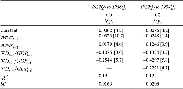
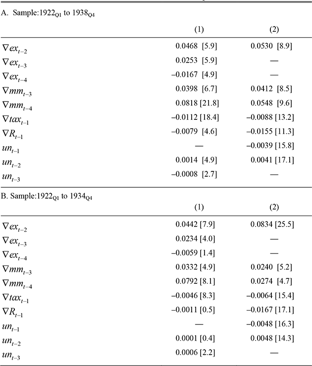
In each case, we report estimates based on a final specification, in which insignificant variables have been deleted (see Table 3). For the estimated coefficients of the included control variables, see Appendix Table 1, column 1. Throughout we use standard errors robust to possible residual autocorrelation and heteroskedasticity, all included variables are significant and the reported equation passes a variety of standard tests for misspecification. The news variable is significantly positive at lags of one and two quarters with coefficients estimated to be, with one-standard error bounds, 0.0325 ± 0.0025 and 0.0179 ± 0.0039.
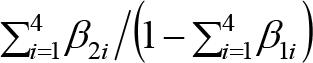
Barro and Redlick's multiplier definition is based on using annual data with single lags of the regressors. Our quarterly counterpart  m = 16\sum\nolimits_{i = 1}^4 {\beta _{1i}} + \sum\nolimits_{i = 1}^4 {\beta _{2i}}. Given the estimates in Table 2, the multiplier is m = 0.45 ± 0.13. For the period truncated at 1934Q4, the estimated multiplier is m = 0.81 ± 0.37.
Since the fit of this equation is not particularly good, with an R 2 of just 0.19, we tried moving to a more general model specification. To this end we relate changes in output growth, ∇ y t, again to lags of news t but now to lags of government spending growth disaggregated into defense and nondefense spending, ∇ dt and ∇non − dt, and lags of nongovernment spending (private expenditure on consumption, investment and net exports) growth, ∇ nt, all growth variables again being defined as one-quarter changes in the logarithms

BARRO AND REDLICK SPECIFICATION ESTIMATES
Note:
Figures in parentheses are robust t-ratios. SE is the regression standard error. The estimates for the ARCH(1) error specification for the equation in column 1 are  \hat \delta _0 = 9.31 \times 10^{ \minus 9} [297.5] and \hat \delta_1 = 1.7016\;[4.2] and are \hat \delta _0 = 5.98 \times 10^{ \minus 9} [241.0 and
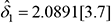 \hat \delta_1 = 2.0891\;[3.7] for the equation in column 2.
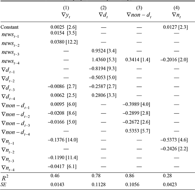
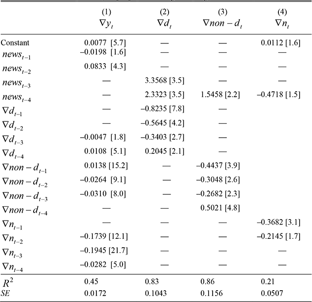
Tables 4A and 4B report our estimates based on a final specification, in which insignificant variables have been deleted. For the estimated coefficients of the included control variables, see Appendix Table 1, column 2.Footnote 16 All included variables are highly significant and the reported equation passes a variety of standard tests for misspecification. The news variable is again significantly positive at lags of one and two quarters with coefficients estimated to be 0.0154 ± 0.0044 and 0.0380 ± 0.0031. The sum annualized of these coefficients (0.213 ± 0.025), may be regarded as an estimate of the “direct” multiplier of defense news on GDP.Footnote 17 The second model offers a superior fit to the Barro and Redlick model, with a much improved R^2 of 0.46 and a regression standard error some 20 percent lower.
However, there may also be “indirect” effects because news may have influence on other various categories of spending that also matter to GDP growth. Regressions of the form  \nabla z_t = \gamma _0 + \sum\nolimits_{i = 1}^4 {\gamma _i \nabla z_{t \minus i} + \sum\nolimits_{i = 1}^4 {\theta _i news_{t \minus i} + v_t}} were therefore estimated for z respectively defined as ∇ d, ∇ non − d, and ∇ n, these being reported in columns 2–4 of Tables 4A and 4B. These were then inserted into equation 2 to obtain a set of indirect multipliers and an overall multiplier, defined as the sum of the direct and indirect multipliers: the time path of the direct and the total overall multipliers are shown in Figure 3. The total overall multiplier is then 0.34 on an annualized basis. It is effectively reached after three years.Footnote 18 For the truncated period ending at 1934Q4, we obtain an annualized total multiplier of 0.76.
Two additional points are worth noting. First, the equation in column 2 shows that defense news does indeed predict subsequent defense expenditure. Second, it should be remembered that ending the sample period at 1934Q4 excludes the defense news data which are subject to relatively large margins of error. This implies that finding a multiplier well below 1 is robust to excluding the largest and least certain values for defense news.
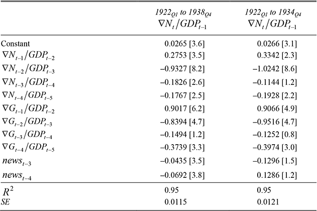
The clear implication is that there was some crowding out of private expenditure even in a “depressed economy.” This issue can be explored using an approach recently proposed by Ramey (Reference Ramey2012). In the current context, Ramey's equation may be specified as

REGRESSION ESTIMATES: PREFERRED SPECIFICATION (sample period: 1922Q1 to 1938Q4)
Notes:
Figures in parentheses are robust t-ratios. SE is the regression standard error. The estimates for the ARCH(1) error specification for the equation in column 1 are  \hat \delta _0 = 2.37 \times 10^{ \minus 7} [322.0] and \hat \delta_1 = 1.5905\,[5.6].
where Nt and Gt are the levels of nongovernment (private) and government expenditure respectively. This equation was estimated for both sample periods and the results are reported in Table 5. Government expenditure has an overall negative effect on private expenditure, with the total impact estimated to be −0.23 for the full sample and −0.28 for the shorter sample.Footnote 19 This confirms that the multiplier, ΔY/ΔG, is < 1 with implied values of 0.77 for the full sample and 0.72 for the shorter sample.
REGRESSION ESTIMATES: PREFERRED SPECIFICATION (sample period: 1922Q1 to 1934Q4)
Note:
Figures in parentheses are robust t-ratios. SE is the regression standard error. The estimates for the ARCH(1) error specification for the equation in column 1 are  \hat \delta _0 = 1.61 \times 10^{ \minus 8} [244.9] and \hat \delta_1 = 1.9243\,[2.7].
THE IMPACT OF REARMAMENT ON GDP
We can use our estimates of the multiplier to examine the impact of rearmament on economic recovery in Britain in the 1930s and compare our findings with those of the best-known paper on this topic by Thomas (Reference Thomas1983). The simplest approach is to take the estimates of the government-expenditure multiplier obtained for the period 1922–1934 and apply them to the increase in defense expenditure of £204 million in 1938. Our multiplier estimate of 0.8 gives a rearmament contribution of about £160 million or 3.3 percent of GDP in 1938. This is half the estimate based on Thomas's method with a multiplier calculated as 1.6 (Ibid.).
DEFENSE NEWS MULTIPLIERS
The idea of “defense news” is that it contains information relevant to private sector decisions. A credible commitment to future defense spending might well stimulate investment by businesses to meet the anticipated demand for military equipment, munitions, etc. Such investment would amount to an element of “crowding in,” and is an example of what the economics literature on the fiscal multiplier would call an anticipation effect.Footnote 20
Some years ago, A. J. Robertson argued that the main initial effect of rearmament was to encourage growth in the construction industry as armaments manufacturers scrambled to add capacity (Robertson Reference Robertson1983). Robertson drew attention to the impact of works and buildings expenditures in, stimulating economic activity and which sustained a vigorous expansion in construction output even as private house-building stalled. Robertson based this argument on the contribution of William Hornby to the official U.K. History of the Second World War (Hornby Reference Hornby1958). Hornby details the buildup of activity to add capacity especially from 1936 onwards. The push included a notable surge in investment for aircraft production and the formation of three important new armaments manufacturing companies. David Chambers's recent compilation of data on all interwar IPOs shows that 20 of the 27 aircraft manufacturing ventures were launched between 1934Q3 and 1936Q2, when the increase in actual defense spending was still relatively small.Footnote 21
ESTIMATING THE EFFECT OF GOVERNMENT EXPENDITURE ON PRIVATE-SECTOR SPENDING
Note:
Figures in parentheses are robust t-ratios. SE is the regression standard error.
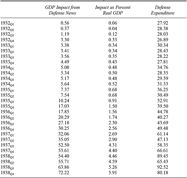
Robertson's view suggests we can use our defense news methodology, which was really designed to facilitate an estimate of the multiplier, to simulate the impact of rearmament on GDP. In principle, the overall multiplier time path from our preferred specification could be used to compute the estimated monetary impact on GDP of defense-news shocks as in Figure 4, which uses a five-year horizon on the basis of a multiplier of 0.34.Footnote 22Figure 4 clearly shows the rapid increase in this impact after 1934, driven by the very large defense-news shocks starting in 1935. Table 6 sets out in more detail the simulated impact of defense news on GDP during the recovery period and also reports actual defense expenditure. Based on the total multiplier (including the direct and indirect components) for the full period, this impact averaged 5.1 percent of GDP in 1938 and amounted to £246.2 million (at 1938 prices) for the four quarters.
SIMULATED EFFECT OF DEFENSE NEWS SHOCKS ON GDP USING A FIVE-YEAR HORIZON
One must be careful not to put too much weight on these estimates because the defense-news shocks in these years were very large. For example, the defense-news shock in 1937Q1 is estimated as £393 million on the basis of the Defense White Paper stating that total defense expenditure over the next five years would be at least £1,500 million. The 1937 announcement was huge compared with the defense news from 1922 to 1934 and compares with actual defense spending in 1936/37 of about half that amount (£194.6 million). Clearly, an impact of 5.1 percent of GDP would entail a very substantial boost to investment from the anticipation effect and is perhaps best regarded as an upper-bound estimate since the increase in investment in manufacturing sectors relevant to the war effort was £57.9 million (at 1938 prices), only £16.5 million more than in 1934.Footnote 23
SIMULATED IMPACT OF DEFENSE NEWS SHOCKS ON REAL GDP (£ million, 1938 prices)
Sources:
Authors' own calculations. See the text and data appendix for GDP and defense expenditure.
Overall rearmament provided a significant stimulus to recovery in the late 1930s. That said, the evidence points to a smaller impact than is found (or implied) by the earlier literature on fiscal multipliers in 1930s' Britain. All this suggests considerable caution before accepting without qualification Thomas's often cited conclusion that “the success of rearmament in creating employment … leads us to view the eschewment of fiscal policy in the thirties as a missed opportunity” (Thomas Reference Thomas1983, p. 571). Our results suggest that, if it is believed that rearmament had a substantial impact, this would be on the basis of the implications of massive future spending plans rather than because there was a large fiscal multiplier. The implication is that a conventional temporary program of expenditure on public works of similar magnitude to the actual increase in defense spending between 1934 and 1938 would have had a much smaller impact on GDP than Thomas's model seems to imply.
DISCUSSION
Both of our econometric models imply that the government expenditure multiplier in interwar Britain was well below 1. A reasonable conclusion from our estimations is that the government expenditure multiplier was between 0.3 and 0.8. This is much lower than the estimates in the historiography reviewed earlier; these ranged between 1.2 and 2.5. As we noted, however, those multipliers were not obtained using modern methods and are clearly questionable. On the other hand, our estimates are quite similar to those found for the United States using a defense-news approach.
There are two reasons as to why the multiplier may have been quite modest even in the 1930s. First, new Keynesian models predict a large multiplier when interest rates are at the “zero lower bound.” In these circumstances, a deficit-financed increase in government spending leads expectations of inflation to increase and the stimulus comes through a fall in the real interest rate. In 1930s Britain the decline in real interest rates was far less dramatic than in the post-gold standard United States.Footnote 24 Second, the legacy of World War I meant that the ratio of public debt to GDP remained above 140 percent and peaked at nearly 180 percent in 1933 (Middleton Reference Middleton2010). Economists have found that, once the level of government debt is over 100 percent of GDP, the response of output to government spending shocks is very small even in deep recessions (Auerbach and Gorodnichenko Reference Auerbach and Gorodnichenko2011). A theoretical reason for this result is that expectations of large tax increases are high when the debt to GDP ratio is high (Perotti Reference Perotti1999). There seems to be stronger modern evidence for consumption reductions stemming from “Ricardian-equivalence” offsets when the debt to GDP ratio is above 100 percent (Rohn Reference Rohn2010).
As Roger Middleton noted, in the 1930s the balanced-budget orthodoxy was strong and extra government spending that threatened fiscal rectitude led to expectations of proximate tax increases (Middleton Reference Middleton1985, chap. 8). Any reader of The Economist's features on public finances and commentary on taxes required to balance the budget would have been painfully aware of the need to raise tax revenues in these circumstances and there were regular changes in income tax rates to this end.Footnote 25 Indeed, in the debate on the budget in 1933, the Treasury publicly maintained that any possible expansionary effects from an unbalanced budget might be vitiated by expectations of future tax increases and that the strong public commitment to the balanced budget rule by government ministers meant that any suggestion of a deficit would lead to expectations of higher taxation.
So some private-expenditure offset to increased defense spending through Ricardian equivalence would not seem unreasonable, especially in a highly unequal economy where income-tax paying classes accounted for a large share of consumption.Footnote 26 The suggestion that news of future defense spending might work to reduce consumption through negative wealth effects is bolstered by Broadberry's estimates of the aggregate consumption function. He finds a significant role for wealth effects.Footnote 27 One should not however jump to the other extreme and conclude that the 1930s recovery in Britain was triggered by the expansionary effects of a fiscal contraction initiated to rescue teetering public finances from the damage of the world economic crisis.Footnote 28 On the contrary, our estimates point to a positive fiscal multiplier, albeit smaller than those of other scholars. They do have the nice property that they echo the views of the British Treasury at the time, namely, that the multiplier was positive but less than 1 (Middleton Reference Middleton1985, p. 163).
So where did recovery come from? Insofar as it was stimulated by policy, the initial phase was based on leaving the gold standard and “cheap money.” The policy stance was developed quite fully by late 1932. It entailed low nominal interest rates and a commitment to raising the price level, underpinned by an exchange-rate target of a 25 percent nominal devaluation compared with the gold standard parity, which was enforced through intervention in the foreign exchange market.Footnote 29 In terms of the overall expansion of real GDP (25.8 percent between 1932Q2 and 1938Q4), our estimates indicate a contribution from rearmament of at most 20 percent, building up mainly after 1935.Footnote 30
The optimism of Keynes and Henderson of the impact of a late 1920s public works program on unemployment has not been shared by quantitative economic historians. They have regarded the claim that a £100 million program for three years would have cut unemployment by 500,000 as implausible. In particular, as Middleton noted, this is mainly because estimates of the multiplier have been lower than those of early Keynesians like Richard Kahn, whose best guess was 1.88, and Keynes himself, who favored a range of 2 to 3 (Middleton Reference Middleton2010; Kahn Reference Kahn1931; Keynes Reference Keynes1933). For example, T. Thomas, whose estimate of the long-run multiplier was 1.44, concluded that by the third year real GDP would be increased by £120 million and unemployment reduced by 329,000 (Thomas Reference Thomas, Floud and McCloskey1994). Dimsdale and Horsewood did support the idea of a relatively large multiplier but their more detailed treatment of the labor market led them to conclude that even though the Keynes-Henderson stimulus would have raised real GDP by £182–£202 million by year three, unemployment would have been reduced only by 302,000–333,000 (Dimsdale and Horsewood Reference Dimsdale and Horsewood1995). Given that to reduce unemployment to “normal levels” in 1932 would have entailed cutting it by close to three million, there is a consensus that at that point there was no possibility of a Keynesian solution to unemployment.
Based on an estimate of 0.8 for the government expenditure multiplier, we are considerably more pessimistic about the impact of the Keynes-Henderson program; Lloyd George would have been hard pressed to cut unemployment by much more than 200,000. So we share the consensus view that it would be unwise to have expected too much from fiscal stimulus in the early 1930s. Moreover, insofar as there were risks that the viability of the cheap money policy could be threatened by announcing a fiscal stimulus which might trigger a rise in risk premia, our results suggest that this gamble was less worth taking than has hitherto been believed.Footnote 31
CONCLUSIONS
We have developed a new approach to estimating the government expenditure multiplier for interwar Britain using quarterly data, time- series econometrics, and defense news announcements. This gives very different results from those found by previous researchers who may not have fully captured the crowding out of private by public expenditure. Our estimates suggest a value in the range 0.3 to 0.8 after three years compared with at least 1.2 in the earlier literature. Evidently, our estimates for the multiplier suggest that there was less scope to use public works to raise GDP and reduce unemployment than has generally been supposed by economic historians and by the early Keynesians. This means that we are in full agreement with earlier writers that “Lloyd George could not have done it,” i.e., that a £100 million pounds program of public works annually for three years would not have reduced unemployment by 500,000 but by 200,000 or less.
Given the circumstances of the early 1930s, we think contemporaries were right to worry that a significant fiscal stimulus would have pushed interest rates up and undermined the cheap money policy which helped to promote recovery in Britain after 1932. If there was such a trade-off between using fiscal or monetary policy to stimulate the economy at that time, then our results tilt the balance further towards relying on monetary policy.
Macroeconomists have become more aware that the magnitude of the multiplier may vary according to the state of the economy.Footnote 32 In that respect, we conjecture that a small multiplier in interwar Britain may reflect the high ratio of public debt to GDP and the worries of private agents that increased government spending might imply large future taxes given the fragility of public finances.
Nevertheless, we find that rearmament delivered a valuable, if limited, stimulus after 1935. Our estimate is that, in the absence of the rearmament program, real GDP in 1938 would have been, at most, 5 percent lower. It is important, however, that for such a large impact to play out would require a large private-sector response to news of massive future defense expenditure rather than coming from a big fiscal multiplier. If a similar amount to that disbursed on defense had been spent on a temporary public works program in the mid-1930s, then based on a multiplier of ≤ 0.8 the boost to real GDP would probably have been no more than a little over 3 percent and the impact on unemployment would have been relatively modest.
Appendix
CONTROL VARIABLE ESTIMATES FROM EQUATIONS 1 AND 2
We report in this Appendix the data sources that we used for the econometric analysis together with the estimated coefficients on the control variables for equations 1 and 2.
Data
The data sources for the variables used in the regressions are as follows:
Real GDP at 1938 prices: Mitchell, Solomou, and Weale Reference Mitchell, Solomou and Weale2012, Table 2b.
Government Expenditure on Goods and Services and on Defense: as reported in The Economist on a quarterly basis at current prices in the first issue of January, April, July, and October each year, converted into 1938 prices using the retail price index from Capie and Collins Reference Capie and Collins1983, table 2.14. Before 1921Q2 defense expenditure was inferred using the annual total reported in Feinstein Reference Feinstein1972, table 33, allocated to quarters based on army numbers taken from General Annual Report on the British Army for years ending 30 September 1920 and 1921.
Defense News: Derived as explained in Crafts (Reference Crafts2012).
Exports: Capie and Collins Reference Capie and Collins1983, table 5.8, converted into 1938 prices.
Tax Rate: Total tax revenues/GDP from Middleton Reference Middleton1996, tables AI.1 and AI.2.
Unemployment: Capie and Collins Reference Capie and Collins1983, table 4.5.
Money Multiplier: M1/monetary base from Capie and Webber Reference Capie and Webber1985, table I.2. Before 1922Q1 M1 was estimated as M3/1.33 from Howson Reference Howson1975 appendix 1, Table 1.
Yield on Consols: Capie and Webber Reference Capie and Webber1985, table III.10.