1 Introduction
Turbulence characteristics in natural bed streams are a fascinating interdisciplinary topic, requiring an integrated approach of experiments and theories to understand the physics of the complex flow structure. The state-of-the-art of research in this field shows that a considerable progress has been made in understanding turbulence in flows over permeable and impermeable rough beds (Kironoto & Graf Reference Kironoto and Graf1994; Dittrich & Koll Reference Dittrich and Koll1997; Nikora & Smart Reference Nikora and Smart1997; Nikora & Goring Reference Nikora and Goring2000; Dey & Das Reference Dey and Das2012). The key characteristic feature that makes the natural bed flow different from the idealised hydraulically smooth or sandy rough flow is the interaction between the flow and the macro-bed roughness. This interaction may occur over a wide range of scales, from fine sediment particle scales to a significant fraction of the flow depth. The largest spatial scales that correspond to the energy-containing eddies are induced by the morphological features, such as bedforms, meandering, braiding or even larger structures such as those of tectonic origin. On the other hand, the smallest spatial scales relate to the so-called dissipative eddies, through which the turbulent kinetic energy (TKE) dissipation occurs owing to viscosity. As observed in natural settings (Roy et al. Reference Roy, Buffin-Bélanger, Lamarre and Kirkbride2004), turbulent flow structures populate the entire flow depth. In between these scales, turbulence is characterised by the net energy coming from the energy-containing eddies being in equilibrium with the net energy cascading to smaller eddies where it is dissipated.
The classical approach to the study of natural bed flows is to compute the time-averaged hydrodynamic quantities, such as the time-averaged streamwise velocity, Reynolds stresses and so on as a function of the vertical distance (along the gravity direction). Importantly, the turbulence statistics for the heterogeneous flow depend on the spatial location. In case of a natural bed flow, such as a pebble bed flow, which can be found in the mountainous rivers and torrents or in watercourses subjected to flash floods and huge sediment transport, or in some reaches where rip-rap layers protect the bed against erosion or local scouring, the time-averaged approach must be supplemented by the spatial averaging approach, especially close to the rough bed where the flow is locally three-dimensional and significantly heterogeneous in space (Nezu & Nakagawa Reference Nezu and Nakagawa1993; Rodriguez & Garcia Reference Rodriguez and Garcia2008). In aerodynamics, such as in canopy flows, the spatial averaging concept was introduced in the 1970s. Monin & Yaglom (Reference Monin and Yaglom1971) defined the spatial averaging methodology as an intricate integral, which has the physical meaning of the averaging over an appropriate space or volume. In hydraulics, spatial averaging was first applied by Smith & McLean (Reference Smith and McLean1977), who considered velocity distributions to average along the lines of equal distance from an undular boundary. In fact, spatial averaging was applied to smooth the vertical distributions of time-averaged hydrodynamic quantities (Wilson & Shaw Reference Wilson and Shaw1977; Raupach & Shaw Reference Raupach and Shaw1982; Finnigan Reference Finnigan1985, Reference Finnigan2000). Subsequently, the double-averaging methodology (DAM) was adopted by applying the spatially averaging approach to time-averaged variables (Antohe & Lage Reference Antohe and Lage1997; de Lemos & Pedras Reference de Lemos and Pedras2001; de Lemos Reference de Lemos2006). Another approach to obtain the double-averaged equations was due to Wilson & Shaw (Reference Wilson and Shaw1977), Raupach & Shaw (Reference Raupach and Shaw1982), Finnigan (Reference Finnigan1985), Giménez-Curto & Corniero (Reference Giménez-Curto and Corniero2002). They took the Reynolds-averaged Navier–Stokes (RANS) equations, which are already time averaged, and supplemented them with spatial averaging or area averaging. Nikora et al. (Reference Nikora, McEwan, McLean, Coleman, Pokrajac and Walters2007) argued that the latter approach is conceptually more transparent and supported by several experimental studies. To be more explicit, the time averaging in DAM is conceptually supplemented by the area averaging in the layer parallel to the mean bed surface (Dey & Das Reference Dey and Das2012). Thus, for macro-rough flows, both temporal and spatial averaging of the fundamental equations and the flow quantities become insightful tools having the potential to provide a better understanding of the turbulence characteristics. In the pioneering work by Nikora et al. (Reference Nikora, Goring, McEwan and Griffiths2001), DAM was proposed for applications in macro-rough bed hydraulics, providing information on the turbulence quantities as a function of vertical distance. The DAM, moreover, allows a measure of additional Reynolds stresses (form-induced stresses) which only appear in the near-bed and interfacial sublayer of macro-rough flows (Nikora et al. Reference Nikora, Goring, McEwan and Griffiths2001; Pedras & de Lemos Reference Pedras and de Lemos2001; Pokrajac, McEwan & Nikora Reference Pokrajac, McEwan and Nikora2008).
Existing experimental results on macro-rough flows indicate that the Reynolds stresses attain their peak values near the crest level of a macro-rough bed. They act as a disturbance to the flow, provoking the generation of turbulence, which weakens away from the source of the disturbance. In this situation, the TKE driving the large eddies (macroturbulence) comes from the mean flow velocity. The large eddies are transformed successively into smaller and smaller eddies in a cascade process with the TKE being transferred from large to small scales, and finally dissipated into heat. Although our understanding in this classical aspect is rather adequate, little is known about the link between the macroscopic turbulence and the laws that govern the dynamics of small-scale turbulence (small eddies). Most of the existing models mainly refer to a set of semi-theoretical relationships to describe the distributions of time-averaged streamwise velocity, Reynolds stresses, TKE budget, turbulence bursting and so on. However, as stated by Keylock, Singh & Foufoula-Georgiou (Reference Keylock, Singh and Foufoula-Georgiou2013), differences in energy transfer close to bedforms can be present, due essentially to intermittent turbulence. These observations imply a reconsideration of the principles on which turbulence closures are based.
In this study, an experiment was conducted to measure the flow field over a highly rough bed. The experimental results are used to verify some robust theorems of hydrodynamics, exploring several laws that involve the third-order moments obtained from the von Kármán–Howarth relations. Finally, to examine the possible causes of the departure of the results of second-order moments from their universal distributions, the characteristics of the helicity in the natural bed flow were analysed. The transport mechanism of second-order moments along the flow depth was also investigated.
This paper is structured as follows. In § 2, the laws of turbulence to be examined in this study are reviewed. The experiment on the natural bed flow is described in § 3, where the distributions of the double-averaged turbulence characteristics are revisited. In § 4, the results on the second-order turbulence statistics are presented, investigating the transition from the energy-containing range to the inertial subrange. In this section, the validity of the Taylor hypothesis is also verified. The third-order laws of turbulence are explored in § 5. In § 6, the role of the kinetic helicity in the turbulent flow system is studied, using the second- and third-order statistics. Finally, discussions and conclusions are summarised in § 7.
2 Laws of turbulence
Turbulence generally involves small-scale isotropic velocity fluctuations (short duration coherent structures) as well as larger-scale anisotropic flows (macroturbulence). The latter can constitute the localised phenomena in the flow; nevertheless, collectively they strongly influence the flow processes (e.g. flow resistance, sediment transport, etc.) related to the small-scale or pure turbulence. Among them, there is the so-called
 $k^{-1}$
scaling law, which is common in several flow situations. More specifically, the energy power spectrum obeys the law
 $$\begin{eqnarray}E(k)\sim k^{-1},\end{eqnarray}$$
where
 $\boldsymbol{k}$
is the wave vector and
 $E(k)$
the spectral energy. The law in (2.1) was derived from the dimensional analysis and asymptotic matching of the inner and outer layers in turbulent boundary layer flows (Perry, Henbest & Chong Reference Perry, Henbest and Chong1986). Different experimental as well as numerical studies, involving the large-eddy simulation (LES) techniques, were performed on atmospheric boundary layer flows to describe the large-scale behaviour of turbulence (Calaf et al.
Reference Calaf, Hultmark, Oldroyd, Simeonov and Parlange2013). Tchen (Reference Tchen1953) was the pioneer in theoretically predicting this scaling by considering a spectral budget, which was later discussed by many authors (Perry & Chong Reference Perry and Chong1982; Marusic et al.
Reference Marusic, McKeon, Monkewitz, Nagib, Smits and Sreenivasan2010; Katul, Porporato & Nikora Reference Katul, Porporato and Nikora2012).
Kolmogorov (Reference Kolmogorov1941a
) introduced the concept of universality in order to mathematically hypothesise the turbulence organization, as well as the concept of characteristic length scales in order to identify an energy-containing range, followed by a universal equilibrium subrange (the so-called inertial subrange). In this way, he further refined the concept of the TKE cascade. At the scales smaller than the largest eddies, the Kolmogorov classical hypotheses of turbulence at high Reynolds numbers permit the assessment of many inertial subrange quantities, specifically the power spectrum
 $E_{u}(k)$
of the streamwise velocity component
 $u$
. It is given by
 $$\begin{eqnarray}E_{u}(k)=C{\it\varepsilon}^{2/3}k^{-5/3},\end{eqnarray}$$
where
 ${\it\varepsilon}$
is the mean TKE dissipation rate per unit mass and
 $C$
the Kolmogorov constant, which is supposed to be universal according to Kolmogorov (Reference Kolmogorov1941a
). Note that in his revised work, this constant depends on the macroscale flow structure (Kolmogorov Reference Kolmogorov1962). Equation (2.2) is the analogous of the
 $2/3$
-law for the second-order structure function in turbulence. The universality of
 $C$
needs to be confirmed experimentally, since it involves a conceptual implication of the intermittency correction. Sreenivasan (Reference Sreenivasan1995) gave a review on the interpretation and the experimental values of the Kolmogorov constant, reporting that the typical values of
 $C$
are of the order of approximately 0.52. Using the Kolmogorov second hypothesis, the TKE dissipation rate is determined from the power spectra in (2.2) (Pope Reference Pope2000; Monin, Yaglom & Lumley Reference Monin, Yaglom and Lumley2007; Dey et al.
Reference Dey, Das, Gaudio and Bose2012; Dey Reference Dey2014). So far, it has been the most reliable way to measure the TKE dissipation rate, even though it involves several uncertainties, because the
 $k^{5/3}$
scaling law and the universality of
 $C$
should be preserved.
Relation (2.2), although providing the turbulent energy spectrum as a function of the wavenumber, is not exact. First, the free coefficients need to be evaluated and, second, corrections due to the multifractal nature of turbulence might affect the exponent (Frisch Reference Frisch1995). Another important aspect is the third-order law, which (given the assumptions) is exact. The hypothesis of three-dimensionally homogeneous isotropic turbulence, limited at high Reynolds numbers, leads to the exact result of the
 $4/5$
-law (Kolmogorov Reference Kolmogorov1941b
)
 $$\begin{eqnarray}\left\langle {\rm\Delta}u^{3}\right\rangle =-\frac{4}{5}{\it\varepsilon}r;\quad {\rm\Delta}u=[\boldsymbol{u}(\boldsymbol{x}+\boldsymbol{r})-\boldsymbol{u}(\boldsymbol{x})]\boldsymbol{\cdot }\frac{\boldsymbol{r}}{|\boldsymbol{r}|},\end{eqnarray}$$
where
 ${\rm\Delta}u$
is the streamwise velocity increment along the increment vector
 $\boldsymbol{r}$
,
 $\boldsymbol{u}$
is the full three-dimensional vector and
 $\boldsymbol{x}$
is the point of location. The angle brackets
 $\langle \boldsymbol{\cdot }\rangle$
denote the double-averaged (DA) value of a quantity. Ensemble averaging is equivalent to time averaging over a sufficiently long period of time in a statistically steady turbulence at a high Reynolds number (Frisch Reference Frisch1995). The law in (2.3) was obtained assuming that the TKE dissipation rate remains constant as kinematic viscosity
 ${\it\nu}$
tends to zero (
 ${\it\nu}\rightarrow 0$
) in the inertial subrange
 ${\it\lambda}_{{\it\eta}}<r<{\it\lambda}_{C}$
. Here
 ${\it\lambda}_{{\it\eta}}$
is the Kolmogorov microscale (dissipation) length and
 ${\it\lambda}_{C}$
the correlation length (see the succeeding sections). It is important to note that, since the TKE dissipation rate
 ${\it\varepsilon}$
is constant throughout the inertial subrange, the large-scale TKE generation rate is equivalent to the small-scale dissipation rate
 ${\it\varepsilon}=2{\it\nu}\langle |\boldsymbol{{\rm\nabla}}\boldsymbol{u}|^{2}\rangle$
. Experimental results revealed that the
 $4/5$
-law is applicable even when the data are analysed in a single direction (Sreenivasan & Dhruva Reference Sreenivasan and Dhruva1998).
The
 $4/5$
-law essentially states the energy conservation in the inertial subrange, i.e. the measure of the TKE flux through scales. The key assumption of the Kolmogorov hypothesis is the local isotropy (or the isotropy at small scales), which holds for high Reynolds number turbulence. In the most general case, the Kolmogorov
 $4/5$
-law can also be obtained for the third-order mixed structure function, expressed as follows in the so-called
 $4/3$
-law:
 $$\begin{eqnarray}\left\langle {\rm\Delta}u|{\rm\Delta}\boldsymbol{u}|^{2}\right\rangle =-{\textstyle \frac{4}{3}}{\it\varepsilon}r.\end{eqnarray}$$
The difference of the above equation from (2.3) is that the total energy of increments
 $|{\rm\Delta}\boldsymbol{u}|^{2}$
is now taken into account, where
 ${\rm\Delta}u$
refers only to the longitudinal increments, as described in (2.3). The above expression can be derived directly from the two-point correlation functions of the RANS equations (Frisch Reference Frisch1995; Antonia et al.
Reference Antonia, Ould-Rouis, Anselmet and Zhu1997). It expresses the nonlinear normal stress fluxes through scales in the inertial subrange as a function of measurable third-order moments. Both the third-order moments in (2.3) and (2.4) arise from the hypothesis of homogeneous isotropic turbulence. They are the exact laws and provide unique information in the inertial subrange, such as characteristic length scales and most importantly, the TKE dissipation (or influx) rate. They require much more precision and effort to have a simple statistical convergence where many datasets are needed. The third-order moments were successfully used to determine and characterize the turbulent cascade in the atmospheric boundary layer flows (Cho et al.
Reference Cho, Anderson, Barrick and Thornhill2001). In addition to homogeneity and isotropy, the main assumptions were stationarity and high flow Reynolds number. Regarding the isotropy, an alternative derivation is anyway possible (Monin & Yaglom Reference Monin and Yaglom1975). It is important to emphasize that the assumption of isotropy may be not verified in many realistic situations, such as in a geophysical turbulence in the presence of physical factors (e.g. rotation and shear layers) which modify the flow dynamics with different invariants and instabilities and break the isotropy condition. Generally, the lack of isotropy renders the derivation of the counterpart of the
 $4/3$
-law far more difficult to obtain.
In analogy to the aforementioned predictions, there are other similar laws related to the so-called helicity, which can play an important role in the dynamics of natural bed flows. The inviscid Navier–Stokes equations (that is the Euler equations) conserve two quadratic invariants, namely the total energy
 $E=\langle |\boldsymbol{u}|^{2}\rangle$
and the mean helicity
 $H=\langle \boldsymbol{u}\boldsymbol{\cdot }{\bf\omega}\rangle$
, where
 ${\bf\omega}=\boldsymbol{{\rm\nabla}}\times \boldsymbol{u}$
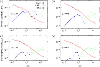
is the vorticity of the flow. The helicity of a localised vortex is a measure of the degree of knottedness of the vortex lines (Betchov Reference Betchov1961; Moffatt Reference Moffatt1969). While total energy was extensively studied especially in statistical theories of turbulence, the aspect of helicity seems to have received little attention in natural bed flows. Direct experimental measurements of helicity are difficult, because it requires information of the local gradients of the velocity components. As an extension of the Kolmogorov hypotheses, the theory of turbulence helicity can play the following roles: (i) a twin TKE cascade and helicity towards smaller scales and (ii) a pure helicity cascade without any TKE transfer. The former was confirmed by the studies of absolute equilibrium ensembles for isotropic helical turbulence and the latter by the two-point closure models of turbulence as well as by the direct numerical simulations (Kraichnan Reference Kraichnan1973; Chen, Chen & Eyink Reference Chen, Chen and Eyink2003; Mininni & Pouquet Reference Mininni and Pouquet2009; Biferale, Musacchio & Toschi Reference Biferale, Musacchio and Toschi2013). In analogy to (2.2), it is expected that in a stationary case, the helicity spectrum behaves like
 $H(k)\sim k^{-7/3}$
(Biferale et al.
Reference Biferale, Musacchio and Toschi2013). Note, moreover, that the role of helicity can be treated in terms of subgrid models for helical turbulence, as reported by Li et al. (Reference Li, Meneveau, Chen and Eyink2006).
Betchov (Reference Betchov1961) first attempted to study the dynamics of helicity, the introduction of which breaks the parity (mirror-image symmetry) of a statistically rotational invariant flow in the simplest symmetrical way. As defined by L’vov, Podivilov & Procaccia (Reference L’vov, Podivilov and Procaccia1997), the mean dissipation of helicity per unit mass and time denoted by
 $h$
is
 $$\begin{eqnarray}h=2{\it\nu}\left\langle (\partial _{i}u_{j})(\partial _{i}{\it\omega}_{j})\right\rangle .\end{eqnarray}$$
The analogous law to the Kolmogorov law can be obtained working on the full correlation tensor. In particular, summarizing briefly, as the main steps, one can define again the streamwise velocity increments as
 ${\rm\Delta}\boldsymbol{u}_{r}=\{[\boldsymbol{u}(\boldsymbol{x}+\boldsymbol{r})-\boldsymbol{u}(\boldsymbol{x})]\boldsymbol{\cdot }\hat{\boldsymbol{r}}\}\hat{\boldsymbol{r}}$
and the transverse component of the velocity as
 $\boldsymbol{u}_{t}=\boldsymbol{u}-u\hat{\boldsymbol{r}}$
(where
 $\hat{\boldsymbol{r}}$
is the wave unit vector). Analogously to the Kolmogorov
 $4/5$
-law (Kolmogorov Reference Kolmogorov1941a
), the so-called
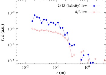
 $2/15$
-law for homogeneous, isotropic turbulence with helicity was derived by Chkhetiani (Reference Chkhetiani1996). It is given by L’vov et al. (Reference L’vov, Podivilov and Procaccia1997), Kurien, Taylor & Matsumoto (Reference Kurien, Taylor and Matsumoto2004) as follows:
 $$\begin{eqnarray}\langle {\rm\Delta}\boldsymbol{u}_{r}(\boldsymbol{x},\boldsymbol{r})\boldsymbol{\cdot }[\boldsymbol{u}_{t}(\boldsymbol{x}+\boldsymbol{r})\times \boldsymbol{u}_{t}(\boldsymbol{x})]\rangle ={\textstyle \frac{2}{15}}hr^{2}\end{eqnarray}$$
being a measure of the helicity flux through a scale of
 $r$
in the inertial subrange. In a statistically steady turbulence it must balance the helicity dissipation
 $h$
in the viscous subrange. The
 $2/15$
-law assumes the behaviour of the inertial subrange of helicity in some scale range. However, it has so far not been measured experimentally or computed by direct numerical simulations. The helicity is indeed quite difficult to quantify even by simulations (Kurien et al.
Reference Kurien, Taylor and Matsumoto2004).
3 Experimentation set-up, double-averaged velocity and second-order moments
The experiments on turbulent flow over a highly rough bed were performed at the Laboratorio ‘Grandi Modelli Idraulici’, Università della Calabria, Italy, in a 1 m wide, 0.8 m deep and 16 m long rectangular tilting flume. Although similarity in the velocity profiles was observed 4 m downstream of the inlet, the test section was located 10 m from the flume inlet. The flume inlet consisted of a stilling tank, an uphill slipway and a honeycomb to damp the residual pump vibrations. An adjustable tailgate was placed at the outlet to set the water depth. Water was collected in a downstream tank, from which it fell in a restitution channel, where another honeycomb and a Bazin weir were placed to measure the discharge before the water entered in the main sump. In the sump, a submerged pump was placed to feed the flume inlet.
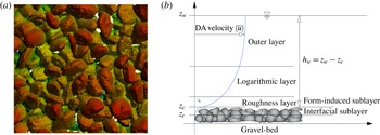
(a) Bed surface detected by a laser scanner and (b) schematic of flow layers.

The hydraulic conditions were fixed at the beginning of the experiment. Namely, the slope was adjusted through a hydraulic jack, while the water depth was set through the downstream tailgate. The discharge was easily kept constant without moving the valves regulating the discharge nor the tailgate regulating the water depth, but only by switching the pump on/off. However, the flow rate was carefully checked during the experiment through the Bazin weir, which has an accuracy of less than
 $2\,\%$
. Non-uniform pebbles with a median size
 $d_{50}=70$
mm were randomly spread to create the rough bed in four layers. The pebble size was widely distributed in a range of diameters from 3 to 10 cm.
The bed surface was captured by a three-dimensional (3-D) laser scanner (Minolta Vivid 300) to characterise the roughness distribution. In order to select a random acquisition window, a
 $0.5\times 0.5~\text{m}^{2}$
wooden frame was randomly placed onto the bed. The frame had the same size as the acquisition window of the laser scanner. Then, the bed surface was acquired inside the wooden frame. The problems of shadow cones were avoided by taking more images by the laser scanner pointed from different positions and merging the acquisitions to obtain a realistic 3-D bed topography with
 $0.1\times 0.1$
mm
 $^{2}$
for the detected spacing points (figure 1
a). A comparison amongst the measurements acquired with the point gauge, through the water displacement method (Dey & Das Reference Dey and Das2012) and with laser scanner, confirmed that the latter gave the best result in terms of precision and resolution of the measured points. Note that the estimation of the
 ${\it\phi}$
-function (
 $=A_{f}/A_{0}$
, where
 $A_{f}$
is the area occupied by the fluid at a given elevation within the total area
 $A_{0}$
for averaging) by using a point gauge or an overhead scanner, was only suitable for the upper
 $70\,\%$
of the interfacial sublayer (Aberle Reference Aberle2007). Non-zero
 ${\it\phi}$
could be obtained with the water displacement method as demonstrated by Dey & Das (Reference Dey and Das2012) who verified the suitability of
 ${\it\phi}$
up to
 $70\,\%$
of the interfacial sublayer. However, as no velocity measurement were taken below
 $70\,\%$
of the interfacial sublayer, the
 ${\it\phi}(z)$
-curve in figure 3 was used satisfactorily. A flow depth
 $h_{w}$
(above the roughness crest level) of 0.2 m, which was measured with a point gauge with decimal Vernier, and a depth-averaged flow velocity
 $U$
of
 $0.261~\text{m}~\text{s}^{-1}$
over the pebble bed slope
 $S$
of 0.00025 were maintained during the experiment. The flow condition did not produce any motion of the pebbles at the bed surface. The average shear velocity
 $u_{\ast }$
obtained from the Reynolds shear stress (RSS) profiles was used to scale the flow and the turbulence quantities. The shear velocity
 $u_{\ast }$
was extracted from the RSS profiles as
 $u_{\ast }=\sqrt{\langle \overline{{\it\tau}}\rangle _{max}/{\it\rho}}=0.024~\text{m}~\text{s}^{-1}$
, where
 $\langle \overline{{\it\tau}}\rangle _{max}$
is the maximum value of the DA total shear stress defined later in (3.1), and
 ${\it\rho}$
is the mass density of fluid. This value is quite close to the value of
 $u_{\ast }=(gh_{w}S)^{0.5}$
, where
 $g$
is the gravity acceleration, obtained using the bed slope as
 $0.022~\text{m}~\text{s}^{-1}$
. The shear Reynolds number
 $R_{\ast }=(u_{\ast }k_{s})/{\it\nu}$
, where
 $k_{s}$
is the roughness parameter (defined later) is estimated as 400, ensuring the hydraulically rough turbulent flow regime. Moreover, we computed the momentum thickness Reynolds number
 $R_{{\it\theta}}=6132$
and the Taylor microscale Reynolds number defined as
 $R_{{\it\lambda}}=u_{\ast }{\it\lambda}_{T}/{\it\nu}\sim 250$
. In the latter
 ${\it\lambda}_{T}\sim 0.01$
m is the Taylor microscale (see § 4). From these characteristic values of the Reynolds numbers, a moderately high turbulent regime was prevalent.
A four-beam down-looking acoustic Doppler velocimeter (ADV) probe (Nortek Vectrino) was used to measure the 3-D instantaneous velocity components (streamwise,
 $u$
, spanwise,
 $v$
and vertical,
 $w$
, with fluctuations
 $u^{\prime }$
,
 $v^{\prime }$
and
 $w^{\prime }$
, respectively). The Vectrino transmitting length was 0.3 mm, the sampling length 1 mm. The data sampling rate and the sampling duration were 100 Hz and 300 s, respectively, which were found to be adequate in order to achieve the statistically time-independent turbulence quantities, as obtained by Dey & Das (Reference Dey and Das2012). The above sampling time corresponds to approximately 600 integral times, with the latter defined as the integral of the autocorrelation function (see § 4). The four-beam Vectrino system has a redundancy for the
 $w$
components, since two components
 $w_{1}$
and
 $w_{2}$
were simultaneously measured by two beams. The variance
 ${\it\sigma}_{z}^{2}$
of the noise is expressed as
 ${\it\sigma}_{z}^{2}=0.5({\it\sigma}_{z1}^{2}+{\it\sigma}_{z2}^{2})$
, where
 ${\it\sigma}_{z1}^{2}=\overline{w_{1}^{\prime }w_{1}^{\prime }}-\overline{w_{1}^{\prime }w_{2}^{\prime }}$
and
 ${\it\sigma}_{z2}^{2}=\overline{w_{2}^{\prime }w_{2}^{\prime }}-\overline{w_{1}^{\prime }w_{2}^{\prime }}$
. It was considered that the data with
 ${\it\sigma}_{z}^{2}<0.3\overline{w_{1}^{\prime }w_{2}^{\prime }}$
had no noise, as they corresponded satisfactorily to the signal correlations greater than 70. Before processing the ADV data for analysis, spikes were detected by using the ellipsoid method proposed by Goring & Nikora (Reference Goring and Nikora2002). However, they were not replaced by any interpolation, but were removed from the samples. We did not adopt the artificial interpolation technique to replace them for such a delicate small-scale turbulence analysis, as in the Kolmogorov third-order scaling laws. However, for some sample datasets, it was verified that the interpolation technique did not significantly alter the results as presented here.
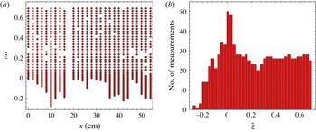
(a) Array of the measuring points on the
 $x\hat{z}$
-plane (measuring points within the pebbles was each 3 mm and above the crest of the pebbles was each 5 mm) and (b) histogram of the measuring points as a function of the normalised elevation
 $\hat{z}$
.

Flow measurements were done in a two-dimensional (2-D) vertical plane (
 $x\hat{z}$
-plane) of the flow, where
 $x$
is the streamwise axis starting from the beginning of the measurement window (10 m downstream of the flume inlet) and
 $\hat{z}=z/h_{w}$
is the normalised elevation above the roughness crest level,
 $z$
being the vertical axis. In the plane of the measurements, along the flume centreline, the effect of the side walls of the flume was negligible. According to Dey & Das (Reference Dey and Das2012) and in order to statistically fulfil the requirements for the heterogeneity, a large number of flow measurements were taken at various streamwise locations along the vertical line. The spatial resolution between two measuring locations (two vertical lines of measurements) was 2 cm, that was well correlated with the roughness length scales
 $k_{s}=17.62$
mm (as specified later). In particular, the convergence of all the moments was verified, computing running averages over the streamwise direction
 $x$
(not shown here).
The grids of measuring points on the
 $x\hat{z}$
-plane are shown in figure 2(a). The deepest measurement was possible below the roughness crest level at
 $\hat{z}=-0.28$
. Figure 2(b) shows the histogram of the measuring points as a function of the elevation
 $\hat{z}$
. It is evident that in the interfacial sublayer the density of measurements was approximately 10, whereas in the wall shear layer the density for each altitude was approximately 30. This ensured that a statistical convergence of the turbulence quantities was achieved (Dey & Das Reference Dey and Das2012). Note that, at the crest elevation, since we intensified the measurements along the vertical axis, more than one sampling fell into the class of the histogram reported in figure 2(b). This fact results into a peak of the distribution (
 ${\sim}50$
measurements) at
 $\hat{z}=0$
.
In natural bed flows, it is convenient to describe the flow by dividing it in different layers with their own flow characteristics. A commonly accepted classification was provided by Nikora et al. (Reference Nikora, Goring, McEwan and Griffiths2001), where the flow depth was divided into three main layers, as shown in figure 1(
 $b$
). They proposed the following classifications of the flow layers:
-
(a) Outer layer: characterised by velocity that is near invariant of the vertical distance due to the presences of large-scale turbulence producing a strong mixing of fluid. The effects of roughness elements are negligible.
-
(b) Logarithmic layer (or wall shear layer): characterised by the universal logarithmic law (log-law). The effects of roughness elements weakly influence the log-law.
-
(c) Roughness layer (or inner layer): in this layer, the effects of roughness elements are predominant. This layer is subdivided into two sublayers:
-
(i) form-induced sublayer, which is influenced by the roughness elements over the element crests;
-
(ii) interfacial sublayer, which consists of flow within the roughness elements and hence is directly influenced by the roughness elements.
-
Figure 1(b) schematically shows the classifications of the flow layers. It is evident that the volume occupied by the fluid depends on the layers above or below the roughness elements. Thus it is important to figure out the fractional space available for the fluid to apply the DAM. In each layer, a generic instantaneous hydrodynamic quantity
 $f(\boldsymbol{x},t)$
, can be decomposed as a time-averaged part
 $\bar{f}(\boldsymbol{x})=T^{-1}\int _{T}\bar{f}(\boldsymbol{x},t)\,\text{d}t$
and a fluctuating part
 $f^{\prime }(\boldsymbol{x},t)=f(\boldsymbol{x},t)-\bar{f}(\boldsymbol{x})$
where
 $t$
is time and
 $T$
the total sampling time. In the DAM, the volume averaging is substituted by an area averaging, considering a thin slab of layer. Hence, a further decomposition in space (with thin thickness) due to the heterogeneity in the fluid layer is possible. The double-averaged quantity
 $\langle \bar{f}\rangle =A_{f}^{-1}\int \bar{f}(\boldsymbol{x})\,\text{d}A$
provides an averaging of time-averaged quantities over an area of fluid
 $A_{f}$
, where
 $\text{d}A$
is an infinitesimal area element. Finally, making use of both time and area averaging, the spatial perturbations are given by
 $\tilde{f}=\bar{f}-\langle \bar{f}\rangle$
. For a steady, zero-pressure gradient flow over a rough bed, the DA RANS equations provide a new definition for the DA total shear stress
 $\langle \bar{{\it\tau}}\rangle$
of fluid in the streamwise direction (Giménez-Curto & Lera Reference Giménez-Curto and Lera1996; Nikora et al.
Reference Nikora, Goring, McEwan and Griffiths2001):
 $$\begin{eqnarray}\left\langle \bar{{\it\tau}}\right\rangle =-{\it\rho}\langle \tilde{u} \tilde{w}\rangle -{\it\rho}\langle \overline{u^{\prime }w^{\prime }}\rangle +{\it\rho}{\it\nu}\frac{\text{d}\langle \overline{u}\rangle }{\text{d}z},\end{eqnarray}$$
where
 $-{\it\rho}\langle \tilde{u} \tilde{w}\rangle$
is the DA form-induced shear stress (FISS),
 $u$
and
 $w$
are the instantaneous streamwise and vertical velocities, respectively,
 $-{\it\rho}\langle \overline{u^{\prime }w^{\prime }}\rangle$
the DA Reynolds shear stress and
 ${\it\rho}{\it\nu}\,\text{d}\langle \overline{u}\rangle /\text{d}\hat{z}$
the DA viscous shear stress. In turbulent flows, the viscous shear stress in (3.1) is negligible across the flow depth. Above the roughness layer, the RSS dominates the FISS (that is inductive stress). The latter contributes predominantly to
 $\langle \bar{{\it\tau}}\rangle$
, mainly within the interfacial sublayer and slightly within the form-induced layer.
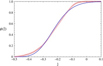
Roughness geometry function
 ${\it\phi}(\hat{z})$
of the experimental bed (open bullets) and comparison with the cumulative probability density function obtained from the gamma distribution (solid line) given by (3.2) used to find the statistical values such as
 $k_{s}$
, etc.

Below the roughness crest level (
 $\hat{z}\leqslant 0$
), the roughness geometry function
 ${\it\phi}(\hat{z})$
is used as a multiplier of an intrinsic DA flow quantity contributing to a superficial DA flow quantity (Aberle Reference Aberle2007; Dey & Das Reference Dey and Das2012). The
 ${\it\phi}(\hat{z})$
that influences the DA estimations is a statistical function depending on the size and shape of the bed sediments. For a heterogeneous gravel bed, a Gaussian distribution describes satisfactorily the statistical variables (mean, standard deviation, skewness and so on; Dey & Das Reference Dey and Das2012). We found that such a distribution is not adequate to describe the heterogeneous pebble bed. In addition, the definition of the statistical distribution describing the bed was used in the present work only to find the values of the mean, standard deviation, skewness, etc., because such values could be ambiguous without a mathematical description. However, the experimental data of roughness are used in the following analysis. In this study, for the heterogeneous natural pebbles, the
 ${\it\phi}(\hat{z})$
can be well described by a gamma distribution:
 $$\begin{eqnarray}{\it\phi}(\hat{z})=\int _{0}^{\hat{z}}{\it\Gamma}(\hat{z})\,\text{d}\hat{z};\quad {\it\Gamma}(\hat{z})=\frac{b^{a}}{{\it\Gamma}(a)}\hat{z}^{a-1}\text{e}^{b\hat{z}};\,{\it\Gamma}(a)=\int _{0}^{\infty }\hat{z}^{a-1}\text{e}^{b\hat{z}}\,\text{d}\hat{z},\end{eqnarray}$$
where
 ${\it\Gamma}$
is the gamma function,
 $a$
is the shape parameter and
 $b$
is an inverse scale parameter. The standard deviation is
 $k_{s}=a^{0.5}b=17.62$
mm. The
 ${\it\phi}(\hat{z})$
in this study is therefore different from the Gaussian distribution as obtained by Dey & Das (Reference Dey and Das2012). The reason of the difference is attributed to the different types of bed roughness. In the present study, the sediments were non-uniform natural pebbles, while in Dey & Das (Reference Dey and Das2012), the sediments were approximately round-shaped uniform gravel.
In figure 3, the variations of the measured
 ${\it\phi}$
from the expectation in (3.2) with non-dimensional vertical distance
 $\hat{z}$
are shown. The measured results and the computed curve have a good agreement.
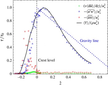
The variations of the shear stresses with
 $\hat{z}$
.

In (3.1), all the shear stresses can be made non-dimensional by dividing by
 ${\it\rho}u_{\ast }^{2}$
and can be expressed as a function of the non-dimensional vertical distance
 $\hat{z}$
. The non-dimensional DA Reynolds shear stress
 $-\langle \overline{u^{\prime }w^{\prime }}\rangle /u_{\ast }^{2}$
is estimated from the experimental data, as shown in figure 4. It is obvious that above the roughness crests (
 $\hat{z}>0$
) the main contribution to the DA total shear stress comes from the DA Reynolds shear stress
 $-{\it\rho}\langle \overline{u^{\prime }w^{\prime }}\rangle$
, as suggested for non-uniform flow (Lim & Yang Reference Lim and Yang2006; Yang & Chow Reference Yang and Chow2008; Manes, Poggi & Ridolfi Reference Manes, Poggi and Ridolfi2011). The
 $-\langle \overline{u^{\prime }w^{\prime }}\rangle /u_{\ast }^{2}$
attains a peak close to the crest level
 $\hat{z}=0$
and shows a sharp damping within the interfacial sublayer (
 $\hat{z}<0$
). It also gradually decreases with an increase in
 $\hat{z}$
above the crest level (
 $\hat{z}>0$
). In the interfacial sublayer, the
 $\langle \overline{u^{\prime }w^{\prime }}\rangle /u_{\ast }^{2}$
is compensated by the form-induced shear stress
 $-\langle \overline{\tilde{u} \tilde{w}}\rangle /u_{\ast }^{2}$
(figure 4). The
 $-\langle \overline{\tilde{u} \tilde{w}}\rangle /u_{\ast }^{2}$
, that has a threshold point slightly above the roughness crest level, increases within the form-induced sublayer up to
 $\hat{z}=0.1$
and then decreases with further decrease in
 $\hat{z}$
. It may be pointed out that the viscous and form-induced shear stresses are negligible above the roughness layer. Thus, the
 $-\langle \overline{u^{\prime }w^{\prime }}\rangle /u_{\ast }^{2}$
is the governing shear stress across the main flow layer (Nikora et al.
Reference Nikora, Goring, McEwan and Griffiths2001; Mignot, Barthelemy & Hurther Reference Mignot, Barthelemy and Hurther2009; Dey & Das Reference Dey and Das2012). In fact, the total stress obtained from the experimental results is not very accurately represented by the linear law of the total shear stress
 $\langle \bar{{\it\tau}}(\hat{z}\geqslant 1)\rangle /({\it\rho}u_{\ast }^{2})=1-\hat{z}$
over the entire layer. This feature is not very uncommon in macro-rough flows (Nikora et al.
Reference Nikora, Goring, McEwan and Griffiths2001). Nikora et al. (Reference Nikora, Goring, McEwan and Griffiths2001) proposed a classification of the flow type, in terms of the roughness height
 ${\it\delta}$
, as follows:
-
(i) Type 1, for
 $H\gg {\it\delta}$
(high relative submergence), where
$H$
is the maximum water depth (distance between the troughs of the roughness elements and the water surface) and
${\it\delta}=3k_{s}$
.
-
(ii) Type 2, for
$(2{-}5){\it\delta}>H>{\it\delta}_{t}$
, which is characterised by eddies produced in the wakes of the roughness having scale
${\it\delta}_{t}$
(thickness of the boundary between the log and linear flow regions). Nikora et al. (Reference Nikora, Goring, McEwan and Griffiths2001) asserted that the linear velocity distribution is valid over the entire depth of such flow type. Nevertheless, Manes, Pokrajac & McEwan (Reference Manes, Pokrajac and McEwan2007) suggested that a simultaneous presence of roughness layer, overlap and outer layers may occur. -
(iii) Type 3, for
$H<{\it\delta}_{t}$
, which presents a low relative submergence. The roughness elements occupy the entire flow depth. In this layer, a universal velocity law is not found.


Our experiment was of flow Type 2, which reveals an unclear boundary to establish if the log-law holds.
 $\langle \bar{u}\rangle /u_{\ast }$
as a function of
 $\hat{z}$
.

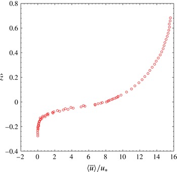
Figure 5 shows the vertical distribution of non-dimensional DA streamwise velocity. In the range of
 $\hat{z}>0$
, the
 $\langle \bar{u}\rangle /u_{\ast }$
distribution exhibits a shear flow similar to that in open channel flows. An interesting feature is however noticeable in the interfacial sublayer
 $-0.08\leqslant \hat{z}\leqslant 0$
where
 $\langle \bar{u}\rangle /u_{\ast }$
varies almost linearly with
 $\hat{z}$
, which is in conformity with Nikora et al. (Reference Nikora, McEwan, McLean, Coleman, Pokrajac and Walters2007). Below
 $(\hat{z}\leqslant -0.08)$
, a depth invariant
 $\langle \bar{u}\rangle /u_{\ast }$
having near-zero value is prevalent owing to the horizontal ground water type of flow.
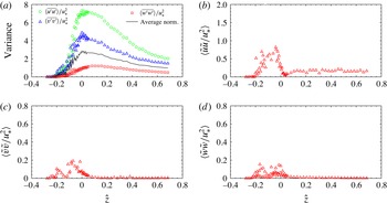
(a) The variation of non-dimensional DA normal stresses with
 $\hat{z}$
and (b), (c) and (d) the non-dimensional form-induced normal stresses.

The variations of non-dimensional DA normal stresses
 $\langle \overline{u_{j}^{\prime }u_{j}^{\prime }}\rangle /u_{\ast }^{2}$
with
 $\hat{z}$
are shown in figure 6(a). It is evident that the
 $\langle \overline{u_{j}^{\prime }u_{j}^{\prime }}\rangle /u_{\ast }^{2}$
-distributions exhibit a similar characteristic. They increase rapidly within the form-induced sublayer with an increase in
 $\hat{z}$
and attain a peak at the top of the roughness crest level. Above the crest level, all distributions have a reduction with an increase in
 $\hat{z}$
with a sequence of magnitude
 $\langle \overline{u^{\prime }u^{\prime }}\rangle >\langle \overline{v^{\prime }v^{\prime }}\rangle >\langle \overline{w^{\prime }w^{\prime }}\rangle$
. It suggests that near the crest level, a mixing process in the presence of roughness elements has the effect of increasing
 $u^{\prime }$
,
 $v^{\prime }$
and
 $w^{\prime }$
. However, there is a damping in the turbulence level within the interfacial sublayer, causing a reduction of
 $\langle \overline{u_{j}^{\prime }u_{j}^{\prime }}\rangle /u_{\ast }^{2}$
. Figure 6(a) also shows the non-dimensional DA TKE
 $(\langle \overline{v^{\prime }v^{\prime }}\rangle +\langle \overline{w^{\prime }w^{\prime }}\rangle )/(2u_{\ast }^{2})$
, which is approximately 0.5 times the non-dimensional DA normal stress or equals the non-dimensional DA TKE in the streamwise direction. This anisotropy factor is used in the discussions of the TKE cascade in succeeding sections. In figure 6(b–d) the distributions of form-induced normal stresses,
 $\langle \tilde{u} \tilde{u} \rangle /u_{\ast }^{2}$
,
 $\langle \tilde{v}\tilde{v}\rangle /u_{\ast }^{2}$
and
 $\langle \tilde{w}\tilde{w}\rangle /u_{\ast }^{2}$
, respectively are shown. They attain peak values within the interfacial sublayer. This feature is similar to the form-induced shear stress and comparable with that obtained by Mignot et al. (Reference Mignot, Barthelemy and Hurther2009) and Dey et al. (Reference Dey, Das, Gaudio and Bose2012).
4 Second-order statistics of turbulence
The second-order statistics of turbulence are analysed by the correlation function and the power spectra of the velocity fluctuations. Using the DAM, we extracted important information on the turbulence dynamics and computed the statistics across the flow depth. In case of a turbulent flow for a given time-averaged velocity, the flow autocorrelation function at a given point
 $\boldsymbol{x}$
can be defined as
 $$\begin{eqnarray}R(\boldsymbol{x},{\it\tau})=\overline{u_{i}^{\prime }(\boldsymbol{x},t)u_{i}^{\prime }(\boldsymbol{x},t+{\it\tau})}.\end{eqnarray}$$
Note that we keep the spatial dependence because of the heterogeneous pebble bed. In our set of measurements
 $\boldsymbol{x}=(x,\hat{z})$
. Using the so-called Taylor hypothesis, we can transform time lags into space increments, namely
 $r=|\overline{u}|{\it\tau}$
(where the time-averaged velocity is a function of
 $\hat{z}$
). With the transformation
 $R(\boldsymbol{x},{\it\tau})\rightarrow R(\boldsymbol{x},r)$
, in the case of statistical convergence, the correlation length is defined as
 $$\begin{eqnarray}{\it\lambda}_{C}(\boldsymbol{x},r)=\frac{1}{R(\boldsymbol{x},0)}\int _{0}^{\infty }R(\boldsymbol{x},r)\,\text{d}r.\end{eqnarray}$$
We computed the correlation length using the experimental data from (4.2) for different positions
 $x$
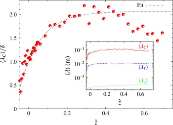
, as represented in figure 2(a). The correlation length is an indication of the size of the biggest eddies in the turbulent flow. This length here is approximately 0.1 m, which corresponds to an integral time of approximately 0.5 s. Similarly to the macroscopic characteristics of the flow, such as the Reynolds stresses and the time-averaged velocity distributions, we also applied the DAM for the characteristics of spectra of turbulence to measure
 $\langle {\it\lambda}_{C}(r)\rangle _{(\hat{z})}$
(by averaging essentially in the horizontal direction
 $x$
). The non-dimensional averaged energy-containing scale
 $\langle {\it\lambda}_{C}\rangle /{\it\delta}$
, namely the typical size of the biggest vortices, depends on
 $\hat{z}$
as shown in figure 7. It increases with an increase in
 $\hat{z}$
up to
 $\hat{z}\approx 0.35$
and then decreases with a further increase in
 $\hat{z}$
. The effects of interface are responsible for this trend. Analogously, in order to verify whether there is scale separation between large energy injecting scales and small dissipative wavelengths, we computed the Taylor microscale
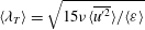 $\langle {\it\lambda}_{T}\rangle =\sqrt{15{\it\nu}\langle \overline{u^{\prime 2}}\rangle /\langle {\it\varepsilon}\rangle }$
. Moreover, we computed the Kolmogorov dissipation length
 $\langle {\it\lambda}_{{\it\eta}}\rangle =({\it\nu}^{3}/\langle {\it\varepsilon}\rangle )^{1/4}$
, comparing it with the energy-containing scale
 $\langle {\it\lambda}_{C}\rangle$
and the typical size of the smallest eddies
 $\langle {\it\lambda}_{T}\rangle$
, as a function of
 $\hat{z}$
, in the inset of figure 7. As it can be seen, there is more than one order of magnitude between these lengths, guaranteeing inertial range turbulence.
Energy-containing scale
 $\langle {\it\lambda}_{C}\rangle /{\it\delta}$
as a function of
 $\hat{z}$
(red points) and a fit type
 $\langle {\it\lambda}_{C}\rangle /{\it\delta}\sim A+B(1-\text{e}^{-{\it\gamma}\hat{z}})$
(dotted black), where
 $A$
and
 $B$
are coefficients. In the inset, the main characteristic scales of turbulence are compared (in metres), namely
 $\langle {\it\lambda}_{C}\rangle$
(full red), the Taylor microscale
 $\langle {\it\lambda}_{T}\rangle$
(dashed blue) and the Kolmogorov dissipation length
 $\langle {\it\lambda}_{{\it\eta}}\rangle$
(dotted green).

Note that a growth of scales towards the free surface is usually typical of natural rivers (Sukhodolov, Thiele & Bungartz Reference Sukhodolov, Thiele and Bungartz1998). On average, the integral scales of turbulence in rivers are as large as the flow depth, but in the present study the average size of pebbles provides the characteristic size.
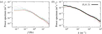
(a) Power spectra
 $E_{u}(f,\boldsymbol{x})$
, at a given
 $\hat{z}$
, for different streamwise distances
 $x$
. (b) Power spectra
 $E_{u}(k,\boldsymbol{x})$
(using the Taylor hypothesis), for different
 $x$
, showing spatially averaged
 $\langle E_{u}(k,\hat{z})\rangle$
(black thick line).

To examine the possible signature of the cascade, we analyse now the power spectra of the streamwise velocity
 $u$
. In particular, we make use of the Blackman–Tukey method to estimate the spectra (Blackman & Tukey Reference Blackman and Tukey1958; Matthaeus & Goldstein Reference Matthaeus and Goldstein1982). Analogously to (4.1), we computed
 $R_{u}(\boldsymbol{x},{\it\tau})=\overline{u^{\prime }(\boldsymbol{x},t+{\it\tau})u^{\prime }(\boldsymbol{x},t)}$
. Then, we took the Fourier transform of the above autocorrelation function, convolved with a Hann window, obtaining the spectrum
 $E_{u}(f,\boldsymbol{x})\equiv E_{u}(f,x,\hat{z})$
as a function of the frequencies. This power spectrum is depicted in figure 8(a) for different streamwise locations
 $x$
at the vertical distance
 $\hat{z}=0.36$
. It is apparent that the power spectra are very similar for different streamwise positions
 $x$
at a given
 $\hat{z}$
, indicating a certain degree of similarity in the power spectra in the streamwise direction in the wall shear layer. Using the Taylor frozen-in hypothesis given by
 $k=f/\langle \overline{u}\rangle _{(z)}$
, we first synchronised the power spectra in the
 $k$
-space, interpolating the Fourier spectra on a fixed
 $k$
-grid, and then we performed a spatial averaging over the streamwise locations
 $x$
. The power spectra as a function of
 $k$
, for several
 $x$
, are reported in figure 8(b), together with the averaged spectrum
 $\langle E_{u}(k,\hat{z})\rangle$
(brackets here mean an average in
 $x$
, as usual). This procedure can be viewed as an extension of the DAM to turbulence measurements. It corroborates a heterogeneous description of turbulence (spectral) quantities in the same manner (that is, double averaging) of large-scale macroscopic moments, such as the Reynolds stresses.
Spatially averaged spectra
 $\langle E_{u}(k{\it\lambda}_{C},\hat{z})\rangle$
for vertical distances
 $\hat{z}=0.21$
and 0.67.

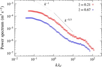
In figure 9 the spatially averaged spectra
 $\langle E_{u}(k{\it\lambda}_{C},\hat{z})\rangle$
are compared for vertical distances
 $\hat{z}=0.21$
and 0.67. Note that we used a proper correlation length to make wavenumbers non-dimensional. The DA spectrum reveals several interesting features. For instance, a large scale for
 $k{\it\lambda}_{C}\leqslant 0.1$
is most likely associated with the non-universal and non-stationary effects along with the effects of the filter window. Also, for
 $10^{-1}<k{\it\lambda}_{C}<10^{0}$
, a
 ${\sim}k^{-1}$
-law type feature is recognised, typical of hydrodynamic turbulence, as discussed in § 2.
The inertial subrange, with a slope quite close to the Kolmogorov expectation
 $-5/3$
, was obtained in the range
 $10^{0}<k{\it\lambda}_{C}<10^{1}$
. We will discuss further this point later in the paper. At scales which correspond
 $k{\it\lambda}_{C}>20$
, a bump is present, which may be related to the presence of a physical effect, such as a secondary inertial subrange (microturbulence at scales smaller than the typical size of the pebbles (Nikora Reference Nikora2008)). Note that similar spectra were observed in channel flows with complex bed topography, where multiscale forcing of the flow can alter the nature of turbulence energy transfer and dissipation (see figure 13 in Keylock et al. (Reference Keylock, Nishimura, Nemoto and Ito2012)). In our case, the non-uniformity of the pebble size introduced other characteristic microscales. In addition, the very high frequencies can be partially affected by noise (from 45 to 50 Hz of Nyquist frequency). We exclude dissipative effects, since, as discussed before, the Kolmogorov length
 ${\it\lambda}_{{\it\eta}}\sim 3\times 10^{-4}$
m is smaller than the resolved scale (
 ${\sim}2\times 10^{-3}$
m.) Finally, at these small scales, realistic effects might be disturbed by the uncertainty in the Taylor hypothesis (see below). Therefore, for the characterization of turbulence properties, we concentrate mostly on the inertial range, from scales
 ${\sim}{\it\lambda}_{C}$
to fractions of the Taylor microscale
 ${\it\lambda}_{T}$
, which indicate the smallest eddies that start being affected by dissipation.
(a) Power spectrum
 $E_{u}$
as a function of
 $k{\it\lambda}_{C}$
at a vertical distance
 $\hat{z}=0.42$
and (b) running slope
 ${\it\alpha}$
as a function of
 $k{\it\lambda}_{C}$
.

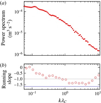
Figure 10(a) shows the power spectrum
 $E_{u}(k)$
of the streamwise velocity
 $u$
at a vertical distance
 $\hat{z}=0.42$
within the wall shear layer. It shows the transition from large to small scales in the inertial subrange of turbulence. A simple way to determine the transition is the computation of the running slope
 ${\it\alpha}=k(\text{d}\log [E_{u}(k)]/\text{d}k)$
, which can be easily obtained from a general guess
 $E(k)=Ak^{-{\it\alpha}}$
, where
 $A$
is a coefficient. The spectrum at
 $\hat{z}=0.42$
is compared in figure 10 with its running slope
 ${\it\alpha}$
. It is evident that at very large scales the slope is quite flat, indicating the presence of very large energy-containing structures (and possibly anisotropic) at scales between a fraction of a metre and of the order of 0.1 m. The
 $k^{-1}$
-law trend arises, as typically observed in many turbulent settings. The existence of a
 $k^{-1}$
-law scaling at low wavenumbers in the streamwise velocity spectrum of wall-bounded turbulence was explained by multiple mechanisms, although experimental support was not so consistent for the laboratory studies (Tchen Reference Tchen1954; Katul & Chu Reference Katul and Chu1998; Katul et al.
Reference Katul, Porporato and Nikora2012). At the wavenumber
 $k_{C}=1/{\it\lambda}_{C}(\hat{z})$
, it can be shown that the injection of energy is approximately
 $$\begin{eqnarray}{\it\varepsilon}(\hat{z})\sim \frac{u_{\ast }^{3}k_{C}(\hat{z})}{{\it\kappa}},\end{eqnarray}$$
where
 ${\it\kappa}$
is the von Kármán constant. Using the results of the experiment of this study, we obtain
 ${\it\varepsilon}\sim 4\times 10^{-4}~\text{m}^{2}~\text{s}^{-3}$
in the range
 $0<\hat{z}<0.2$
. This value will be useful as a rough estimator for the next sections.
At smaller scales, finally, the slope is consistent with a type of Kolmogorov
 $-5/3$
-scaling law. Note that the latter slope is less steep than the
 $-5/3$
expectation, possibly due to intermittency correction (Frisch Reference Frisch1995). Moreover, other effects might influence the Kolmogorov law, such as the presence of finite helicity in the system (next sections), or multiple time scales in the system. The occurrence of an energy spectrum with a slope different from the usual
 $5/3$
-law can be explained using phenomenological characteristics of boundary layer turbulence. Turbulence in natural bed flows is characterised by three main time scales. The first time scale is the usual eddy-turnover time of turbulence at a given length scale
 $\ell$
, namely
 ${\it\tau}_{NL}\sim \ell /{\rm\Delta}u$
. The second time scale is due to the continuous shear flow, because the time-averaged velocity depends on the vertical distance
 $z$
, so
 ${\it\tau}_{s}\sim \ell /u_{\star }$
. Finally, a third time scale is due to the increase of large-scale eddies as a result of mean flow instability; so
 ${\it\tau}_{L}\sim {\it\lambda}_{C}/u_{rms}$
. A moment of reflection is enough to realize that in such a situation, both the increase of large scales and the local shear flow should be responsible for the slowdown of the energy cascade. It is attributed to the fact that the local shear time may happen to be lower than the nonlinear time at a given scale, mainly in the presence of an increase in the large-scale size. In this case, the nonlinear energy cascade at scales of the order of
 $\ell \sim k^{-1}$
is realised in a time
 $T_{\ell }$
, so that the TKE dissipation rate per unit mass is defined as
 ${\it\varepsilon}\sim {\rm\Delta}u^{2}/T_{\ell }$
. As a first approximation, when the effective nonlinear time increases by a factor
 ${\it\tau}_{NL}/{\it\tau}_{s}$
with respect to the eddy-turnover time at that scale and height, say
 $$\begin{eqnarray}T_{\ell }\sim {\it\tau}_{NL}\left(\frac{{\it\tau}_{NL}}{{\it\tau}_{s}}\right),\end{eqnarray}$$
due to the scaling law
 $kE(k)\sim {\rm\Delta}u^{2}$
, one can obtain
 $$\begin{eqnarray}E(k)\sim ({\it\varepsilon}u_{\star })^{1/2}k^{-3/2}.\end{eqnarray}$$
Our conjecture is just a preliminary model to see how some physical effects can easily affect the usual cascade to change the spectral slope with respect to the usual homogeneous and isotropic energy cascade depicted by Kolmogorov (Reference Kolmogorov1941a ). Of course, some other physical effects could be responsible for the observed deviations from the Kolmogorov law for the power spectrum. The anomalous spectrum can also be interpreted in terms of non-equilibrium dissipation for the channel flow, as described by Horiuti & Ozawa (Reference Horiuti and Ozawa2011). Moreover, as described by Keylock et al. (Reference Keylock, Nishimura, Nemoto and Ito2012), departures from the Kolmogorov expectation can be due to direct energy injection at subintegral scales because of multiscale forcing, such as that seen here from a complex bed roughness.
4.1 Validity of the Taylor hypothesis
When measuring the aforementioned quantities in a turbulent flow using the time-resolved single-point measurements, it is challenging to correlate the temporal fluctuations with the spatial ones. The main approximation in experimental turbulence studies is the association with wavenumbers: The frozen-in flow hypothesis proposed by Taylor (Reference Taylor1938), which assumes that the flow field is advected past the probe with a mean flow in a quasi-frozen manner, i.e. the velocity fluctuations evolve slowly as compared to the mean velocity. This naturally restricts its application to low turbulence intensities, namely when the variance of the velocity fluctuations is much smaller than the characteristic mean flow. This is generally true in many systems such as fast winds in atmospheric boundary layer flows, while it is less robust in wall-bounded flows, and ever more challenging in permeable pebble bed flows. For a more concise characterization of the Taylor hypothesis, looking at the space–time variations, several discussions can be found in Del Alamo & Jiménez (Reference Del Alamo and Jiménez2009) and Smits, McKeon & Marusic (Reference Smits, McKeon and Marusic2011). In this study, we propose a simple measure of the
 $k$
-dependent frozen flow. According to Matthaeus & Goldstein (Reference Matthaeus and Goldstein1982), we compare two simple time scales, namely the large-scale advection time and the characteristic nonlinear time. The first is given by:
 $$\begin{eqnarray}{\it\tau}_{\langle \bar{\boldsymbol{u}}\rangle }(k,\hat{z})=\frac{{\it\lambda}}{\langle \bar{\boldsymbol{u}}\rangle _{(\hat{z})}}=\frac{2{\rm\pi}}{k\langle \bar{\boldsymbol{u}}\rangle _{(\hat{z})}}.\end{eqnarray}$$
Such a time, at each scale and vertical position, should be always smaller than the characteristic nonlinear time
 $$\begin{eqnarray}{\it\tau}_{NL}(k,\hat{z})=\frac{1}{k\sqrt{k\langle E(k,\hat{z})\rangle }}.\end{eqnarray}$$
The latter can be viewed as the typical distortion time of eddies of size
 $k$
at a vertical distance
 $\hat{z}$
. The relation that should be satisfied for the frozen flow approximation is
 ${\it\tau}_{\langle \bar{\boldsymbol{u}}\rangle }(k,\hat{z})\ll {\it\tau}_{NL}(k,\hat{z})$
, which can be combined in a single scalar function as
 $$\begin{eqnarray}{\it\psi}(k,\hat{z})=\frac{2{\rm\pi}\sqrt{k\langle E(k,\hat{z})\rangle }}{\langle \bar{\boldsymbol{u}}(\hat{z})\rangle }\ll 1.\end{eqnarray}$$
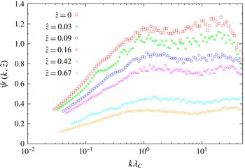
The parameter
 ${\it\psi}(k,\hat{z})$
is shown for several
 $\hat{z}$
in figure 11. It is evident that, very close to the pebble bed, in the injection region (or rough region) of small-scale turbulence, the Taylor hypothesis is violated (
 ${\it\psi}\sim 1$
) at scales of the order of
 ${\it\lambda}_{C}$
. This suggests that the results close to the turbulent boundary layer must be taken with care, especially when they bring in concepts of spatial turbulence such as the Kolmogorov cascade. Note that (4.8), generally, can be used as a statistical tool to verify the frozen-in approximation in a turbulent boundary layer.
Taylor coefficient
 ${\it\psi}(k,\hat{z})$
, as a function of
 $k{\it\lambda}_{C}$
, for different vertical distances
 $\hat{z}$
.

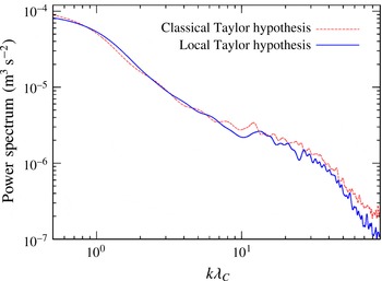
Power spectrum
 $E_{u}(k{\it\lambda}_{C})$
, at
 $\hat{z}=0.03$
. The dashed (red) line is the spectrum computed assuming the global Taylor hypothesis while the full (blue) line represents the same spectrum computed using the local Taylor hypothesis, described by (4.9)–(4.10) (Pinton & Labbé Reference Pinton and Labbé1994). As expected, departure is observed at small scales, for
 $k{\it\lambda}_{C}>10$
.

A possible way to partially reconstruct the field, and also to further test (4.8), is the use of a ‘local Taylor hypothesis’. In a seminal paper by Pinton & Labbé (Reference Pinton and Labbé1994), a modified version of the hypothesis was proposed in order to study swirling flows with single-probe measurements in the absence of mean velocities. Here, we adapt their study to our experimental set-up. For simplicity, and as in the original work (Pinton & Labbé Reference Pinton and Labbé1994), we will restrict ourselves to a simple one-dimensional (1-D) reconstruction, relating in a Lagrangian way the streamwise velocity at a time
 $t$
to a spatial pattern:
 $$\begin{eqnarray}u(t)\rightarrow u(x)~~x=\int _{0}^{t}U(t^{\prime })\,\text{d}t^{\prime },\end{eqnarray}$$
where
 $U$
is a local average velocity (running average):
 $$\begin{eqnarray}U(t)=\frac{1}{T}\int _{t-T/2}^{t+T/2}u(t^{\prime })\,\text{d}t^{\prime },\end{eqnarray}$$
where the time
 $T$
is a multiple of the integral time (which here we chose to be 2 times the integral time, although we verified that the results do not particularly depend on this choice). This ‘sweeping velocity’ is obviously smooth and represents the local velocity with which the flow passes through the probe. When transformations (4.9)–(4.10) are applied, they produce a set of spatial data unevenly sampled. Using adequate second-order numerical interpolation, we reconstruct the field on a regular grid, finally computing the power spectrum
 $E_{u}(k)$
at a given probe position
 $x_{\ast }$
and elevation
 $\hat{z}$
. An example of the this streamwise velocity spectrum is reported in figure 12, where we compare both the global Taylor hypothesis, where
 $k=2{\rm\pi}/[t\overline{u}_{(\hat{z})}]$
, to the above local approximation (4.9)–(4.10). As it can be seen, spectra are indistinguishable in the inertial range, for
 $k{\it\lambda}_{C}<10$
, while a bifurcation is observed at higher frequencies. This departure is due to fast dynamical processes, as previously described. Moreover, comparing this analysis with figure 11, it emerges that the breaking
 $\boldsymbol{k}$
-vector is very similar, further confirming the accuracy of our diagnostic. This technique, although very simple, could be extended to three dimensions, but a more delicate procedure needs to be used and will be therefore investigated in future works.
Note that in the near-bed zone, where the Taylor hypothesis is violated, it might be that the most effective decorrelation mechanism is due to the large-scale random sweeping effects (Tennekes Reference Tennekes1975; Chen & Kraichnan Reference Chen and Kraichnan1989; Nelkin & Tabor Reference Nelkin and Tabor1990; Sanada & Shanmugasundaram Reference Sanada and Shanmugasundaram1992; Praskovsky et al. Reference Praskovsky, Gledzer, Karyakin and Zhou1993). In this case, the Eulerian frequency spectrum should be
 $$\begin{eqnarray}E(f)=C_{E}({\it\varepsilon}u_{rms})^{2/3}f^{-5/3},\end{eqnarray}$$
where
 $u_{rms}$
is the root mean square of the total velocity fluctuations and
 $C_{E}$
is another (possibly non-universal) constant. Note that the above relation is very different from (2.2), since it explicitly depends on the level of fluctuations. Estimation of the TKE dissipation rate close to, or below, the crest of pebbles based on (4.11) may lead to a very imprecise measurement of the TKE dissipation rate. The investigation of the sweeping effects may be related to the presence of helical persistent structures, as we will discuss in the succeeding sections.
5 Third-order laws for turbulence
As discussed in § 2, one of the few exact theorems of turbulence is the Kolmogorov
 $4/5$
-law described by (2.3). From this law, it is straightforward to obtain the averaged TKE dissipation rate as
 $$\begin{eqnarray}\langle {\it\varepsilon}\rangle =-\frac{5}{4r}\left\langle \overline{{\rm\Delta}u^{3}}\right\rangle ,\end{eqnarray}$$
where
 ${\rm\Delta}u=u(\boldsymbol{x}_{\ast },x+r)-u(\boldsymbol{x}_{\ast },x)$
, that is the space increment of the streamwise velocity. The overbar denotes the average within the sample (time average, using the Taylor hypothesis) and the angular brackets represent the DA values over the probe positions
 $\boldsymbol{x}_{\ast }$
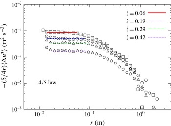
according to the DAM. Note that, to compute the above law, we apply directly the Taylor frozen-in approximation, once the applicability of the hypothesis is verified, in the appropriate range of scales, as described in the previous section. Equation (5.1) can be used to measure, in a precise and unique way, the TKE dissipation rate in any turbulent flow which obeys the RANS equations. The compensated Kolmogorov
 $4/5$
-law, given by (5.1) for different vertical distances
 $\hat{z}$
in a natural bed flow, is shown in figure 13. The fit to (5.1) is shown with horizontal lines. It is found that the law is quite constant for length scales smaller than the correlation length (
 ${\sim}0.1$
m). The law is computed only down to lengths in the inertial subrange. Comparing figure 13 with the inset of figure 7, it is important to note that the law is lost at scales
 $r>\langle {\it\lambda}_{C}\rangle$
, and it persists down to the Taylor microscale
 $\langle {\it\lambda}_{T}\rangle$
, as expected from the statistical theory of turbulence (Frisch Reference Frisch1995).
A further validation of the robustness of the law is undertaken with the comparison of the second-order moments with the power spectrum. The
 $4/5$
-law indeed defines the inertial subrange of turbulence. On the contrary, the
 $5/3$
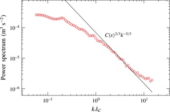
-law is not as robust as the third-order moment, being more sensible to other effects such as non-stationarity, intermittency and so on. However, in well-behaved turbulence, both the laws should be consistent if the hypotheses are satisfied. In this regard, we compare the results between (5.1) and (2.2). The power spectrum of
 $\langle E_{u}(k,\hat{z})\rangle$
at
 $\hat{z}=0.29$
is reported in figure 14, together with the
 $5/3$
-law. The latter, which is applicable in the inertial subrange, was obtained using
 $C=0.52$
, and the dissipation rate
 $\langle {\it\varepsilon}\rangle$
was obtained from (5.1).
Compensated Kolmogorov
 $4/5$
-law in natural bed flow for different vertical distances showing the fit to (5.1) by the horizontal lines.

Power spectrum
 $\langle E_{u}(k,\hat{z})\rangle$
at
 $\hat{z}=0.29$
compared with the Kolmogorov
 $C\langle {\it\varepsilon}\rangle ^{2/3}k^{-5/3}$
line for
 $C=0.52$
.

The value of the Kolmogorov constant
 $C$
was chosen from the literature, in particular from the work by Sreenivasan (Reference Sreenivasan1995). To confirm further, we computed a fit using (2.2), with
 $C$
as a variable, and we obtained
 $C=0.51$
 $\pm 5\,\%$
, indicating that this method of estimation of
 ${\it\varepsilon}$
can be also used to investigate the fluctuations of the universal Kolmogorov constant. As can be seen from figure 14, the TKE dissipation rate from the third-order law fits quite well the power spectrum, indicating that the present procedure is a robust and precise method in order to measure the cascade intensity in natural bed flows, such as in rivers and in the related laboratory experiments.
Alternatively, as shown in (2.4), one can obtain the TKE dissipation rate per unit mass from the
 $4/3$
-law (Frisch Reference Frisch1995; Antonia et al.
Reference Antonia, Ould-Rouis, Anselmet and Zhu1997; Wan et al.
Reference Wan, Servidio, Oughton and Matthaeus2010; Wan et al.
Reference Wan, Servidio, Oughton and Matthaeus2009):
 $$\begin{eqnarray}\langle {\it\varepsilon}\rangle =-\frac{3}{4r}\left\langle \overline{{\rm\Delta}u({\rm\Delta}v_{j})^{2}}\right\rangle =-\frac{3}{4r}\left\langle \overline{{\rm\Delta}u\left[({\rm\Delta}u)^{2}+({\rm\Delta}v)^{2}+({\rm\Delta}w)^{2}\right]}\right\rangle .\end{eqnarray}$$
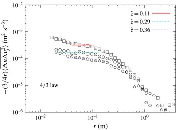
The
 $4/3$
-law, also known as the Monin–Yaglom law for its consistency with the third-order mixed structure function for passive tracers, is shown in figure 15. As can be seen, although the behaviour is very similar to the
 $4/5$
-law (figure 13)), it has slight differences. Firstly, the ranges of the validity of the law are slightly different and somehow smaller. Secondly, the goodness of the fit is not as high as in the
 $4/5$
-law. Finally, the value of the dissipation rate obtained from the
 $4/3$
-law seems to be smaller, as we will discuss below. These differences are due to the nature of turbulence in anisotropic systems and can be directly quantified from both the laws. Indeed the law in (5.2) assumes isotropy, which is only partially certain at small scales in a system like this. As it can be seen from the macroscopic scenario presented before, the variance anisotropy is indeed quite strong at large scale with
 $\langle \overline{u^{\prime }u^{\prime }}\rangle \sim (\langle \overline{v^{\prime }v^{\prime }}\rangle +\langle \overline{w^{\prime }w^{\prime }}\rangle )$
(see figure 6). The anisotropy therefore can be the cause of the variation in scales (different correlation scales in streamwise and normal directions) and in the variation of
 ${\it\varepsilon}$
. The various additional hypotheses needed in the Monin–Yaglom law can be also responsible for the higher uncertainties in the fit. In the latter case,
 ${\it\varepsilon}$
has a typical error of the order of
 $6\,\%$
.
The Monin–Yaglom (
 $4/3$
) law. Compensated Kolmogorov
 $4/3$
-law for turbulence in a turbulent channel with natural bed, for different latitudes. The fit to equation (5.2) is reported in the horizontal (coloured) lines. The errors on the fit are approximately 5–7 %.

For completeness, as a final qualitative estimate, the dissipation rate is measured using the power spectrum. In a Newtonian fluid, the rate at which the TKE is dissipated by viscosity is
 $$\begin{eqnarray}{\it\varepsilon}_{{\it\nu}}=2{\it\nu}\int _{0}^{\infty }k^{2}E(k)\,\text{d}k,\end{eqnarray}$$
where
 $E(k)$
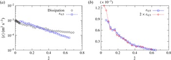
is the total TKE. The TKE dissipation rate, as a rough estimation, is reported in figure 16(a). Note that this measurement can somewhat underestimate the realistic dissipation rate because it might not be free from artefacts of the instrument. Namely it converges only if the Kolmogorov scale is well resolved, that is usually a difficult proposition in experiments. However, evidently the measure of
 ${\it\varepsilon}_{{\it\nu}}$
is comparable with the transfer rate obtained in the inertial subrange from the
 $4/5$
-law. Finally, in figure 16(b), the TKE dissipation rates obtained from the Monin–Yaglom
 $4/3$
-law and the Kolmogorov
 $4/5$
-law are compared. It is clear that the transfer rate from the
 $4/3$
-law is approximately one-half of that of the
 $4/5$
-law. This can be related to the above discussions on the macroscopic anisotropy of turbulence in a natural bed flow.
In the wall shear layer, the spectral slope of the streamwise velocity varies from
 ${\sim}k^{-1.5}$
at
 $\hat{z}\sim 0.05$
to
 ${\sim}k^{-1.3}$
closer to the outer layer, indicating a noticeable discrepancy from the Kolmogorov universal
 $5/3$
spectral slope, as discussed before. This divergence from the so-called Kolmogorov second-order universality can be due to several aspects: firstly, shear layers, which can be quantified from the above Reynolds stresses and velocity profiles, induce anisotropy in the energy cascade (spectral anisotropy), influencing the arguments used in obtaining the scaling law; secondly, the presence of coherent structures and intermittent events which can vary the law. Such a problem is known as non-universality of turbulence (Linkmann et al.
Reference Linkmann, Berera, McComb and McKay2015), which is studied in the succeeding section.
6 Helicity and coherent structures
Coherent structures are the major components of turbulent flows, appearing from scales of the order of
 ${\it\lambda}_{C}$
down to the end of the inertial subrange of turbulence, where the dissipative eddies eventually dominate the dynamics. This picture is here corroborated by performing a scale-dependent kurtosis analysis, which is the topic of future work. The scale-dependent kurtosis goes from a value of the order of 4.5 in the inertial subrange at scales of the order of a centimetre to a Gaussian value of 3 at scales comparable with
 ${\it\lambda}_{C}$
. Coherent structures are eddies which persist in time, and generally they are equilibrium-like solutions of the RANS model. The most common equilibrium is the helical state, in which the velocity and the vorticity (curl of the velocity) tend to align. In order to study the appearance of these phenomena in natural bed flows, we estimated the contribution of helicity to the turbulent cascade by measuring the reduced helicity described as follows.


It is possible to estimate helicity in turbulence using the velocity cross-spectra. The correlation tensor of the velocity is
 $\unicode[STIX]{x1D619}_{ij}^{s}(\boldsymbol{r})+\unicode[STIX]{x1D619}_{ij}^{a}(\boldsymbol{r})$
, where
 $\unicode[STIX]{x1D619}_{ij}^{s}$
and
 $\unicode[STIX]{x1D619}_{ij}^{a}$
are the symmetric and the antisymmetric part of the correlation tensor, respectively. The symmetric part is related to the energy, while the antisymmetric part retains information about the helicity. The above tensor can be represented in Fourier space (Eidelman et al.
Reference Eidelman, Elperin, Gluzman and Golbraikh2014), separating the symmetric and the antisymmetric part as
 $$\begin{eqnarray}\tilde{\unicode[STIX]{x1D619}}_{ij}(\boldsymbol{k})=A(\boldsymbol{k})\left({\it\delta}_{ij}-\frac{k_{i}k_{j}}{k^{2}}\right)+G(\boldsymbol{k}){\it\epsilon}_{ijl}\frac{k_{l}}{k},\end{eqnarray}$$
where
 ${\it\delta}_{ij}$
is the Kronecker tensor and
 ${\it\epsilon}_{ijl}$
is the Levi-Civita antisymmetric tensor. The last term of the right-hand side of (6.1) is related to the helicity density, while the first term is related to the energy. The helicity is given by
 $H=\langle \boldsymbol{v}\times {\bf\omega}\rangle =-(1/2){\it\epsilon}_{ijl}\int \tilde{R}_{il}(\boldsymbol{k})k_{j}\,\text{d}\boldsymbol{k}$
, where
 ${\bf\omega}=\boldsymbol{{\rm\nabla}}\times \boldsymbol{v}$
is the vorticity.
The helicity has not been topic of intensive investigations, both in numerical as well as in experimental studies of turbulent flow in general, and in the case of natural bed flow in particular. The first study of helicity in the context of turbulence was done by Betchov (Reference Betchov1961). He considered the general form of the two-point velocity correlation in a semi-isotropic turbulence, i.e. turbulence which is invariant under rotations but not necessarily under reflections. Obviously, the helicity is a pseudo-scalar quantity fundamentally related to the properties of symmetry of a turbulent flow. As suggested by Brissaud et al. (Reference Brissaud, Frisch, Leorat, Lesieur and Mazure1973), using simple phenomenological and dimensional arguments, it was possible to show that the helicity undergoes a turbulent cascade and the resulting modification of the exponent of the power law of the energy spectrum in a Kolmogorov-type inertial subrange. Numerical simulations and analytical models (Polifke & Shtilman Reference Polifke and Shtilman1989; Chen et al. Reference Chen, Chen and Eyink2003; Mininni & Pouquet Reference Mininni and Pouquet2009) showed that in 3-D turbulence it is possible to have a joint cascade of both energy and helicity to large wavenumbers. With increasing wavenumber, the non-dimensional helicity tends to be zero and is carried along locally and linearly with the energy cascade like a passive scalar.
Power spectrum of the longitudinal components of the velocity field
 $\langle E_{u}(k,\hat{z})\rangle$
(open red circles), and power spectrum of the reduced helicity. The helicity has been distinguished among positive (blue symbols) and negative (open green squares). The large-scale
 $k^{-1}$
behaviour is also reported (black dashed line). Different panels refer to different regions of the flow depth. The
 $y$
axis is in arbitrary units.

(a) Two-dimensional flow in the
 $xz$
-plane; (b) zoom of the
 $(u,w)$
flow in a region of gaps between pebbles, showing the persistent vortical structure; (c) vertical profile of the in plane velocity field
 $v$
, showing that the structures have embedded a net helicity
 $H=\boldsymbol{v}\boldsymbol{\cdot }{\bf\omega}\sim v{\it\omega}_{y}$
; (d) reduced helicity at three fixed positions through the vortex. The positions are highlighted with symbols in (b).

The kinetic helicity modal spectrum can be written as
 $$\begin{eqnarray}h(\boldsymbol{k})=\frac{\tilde{\boldsymbol{u}}(\boldsymbol{k})\boldsymbol{\cdot }\tilde{{\bf\omega}}^{\ast }(\boldsymbol{k})+\tilde{\boldsymbol{u}}^{\ast }(\boldsymbol{k})\boldsymbol{\cdot }\tilde{{\bf\omega}}(\boldsymbol{k})}{2}=\text{i}{\it\epsilon}_{jlm}k_{l}S_{mj}(\boldsymbol{k}),\end{eqnarray}$$
where
 $S_{ij}(\boldsymbol{k})=\tilde{u} _{i}(\boldsymbol{k})\tilde{u} _{j}^{\ast }(\boldsymbol{k})$
. Therefore, the spectrum of
 $h$
explicitly appears in the energy spectrum tensor, and similarly to Matthaeus & Goldstein (Reference Matthaeus and Goldstein1982), integrating along two normal directions, let us say
 $y$
and
 $z$
, one can obtain
 $$\begin{eqnarray}H(k)=2k\text{Im}\,\{S_{yz}^{r}\},\end{eqnarray}$$
where
 $H(k)$
is the reduced helicity, integrated along the spanwise and vertical direction,
 $y$
and
 $z$
respectively,
 $k=k_{x}$
is the
 $\boldsymbol{k}$
-vector along the streamwise direction and
 $S_{yz}^{r}=\tilde{u} _{y}(k)\tilde{u} _{z}^{\ast }(k)=\tilde{v}(k)\tilde{w}^{\ast }(k)$
. According to the DAM and analogously to the power spectra, we averaged the helicity in planes parallel to the bed (essentially in the streamwise direction) for varying
 $\hat{z}$
. The power spectra of energy and helicity are compared for different
 $\hat{z}$
in figure 17. Note that, contrary to the energy, helicity has no definite sign, and the averaging procedure therefore cancels most of the asymmetric contribution to the cascade. Only the strongest helical contribution persists with averaging. Therefore, the spectra in figure 17 have a well-defined meaning. In particular, closer to the induction layer, there is a net amount of helicity at scales of the order of the correlation length (
 $k\sim {\it\lambda}_{C}^{-1}$
), suggesting that the input of energy is accompanied by a swirling motion. The characteristics of this motion will be shown below. At scales much larger than
 ${\it\lambda}_{C}$
(
 $k\ll 10$
m
 $^{-1}$
), the helicity retains the same sign, but reduces dramatically in intensity. This reduction is due to both the real decrease of helicity in the system and the windowing technique for the Fourier spectrum. At small scales, as it is evident in figure 17(a), the helicity starts to alternate sign, which is typical of a random isotropic cascade. At higher elevations in the wall shear layer, the large-scale definite (positive) helicity reduction and a counter rotating smaller eddies develop in the primary inertial subrange. This behaviour is self-similar at higher elevations, at least in the wall shear layer.
The question now raised is: which process introduces this amount of helicity in the system? To answer this question, it is important to fragment our analysis into subportions of the system, breaking (temporarily) the DAM. In this regard, we concentrate on the gap between pebbles, as reported in figure 18. The 2-D flow in the plane
 $xz$
is reported in figure 18(a), showing the main stream in the wall shear layer. Highlighted in this panel, there is a region in a water dip, represented in figure 18(b). The locally averaged structure shown a typical excavating stationary vortex. Note that this whirling structure is very persistent, since averaging measurements were taken over 300 s. The vertical profile of the in plane velocity field
 $v$
is shown in figure 18(c). The geometry of the structure is even clearer, showing that the vortex has embedded a net helicity
 $H=\boldsymbol{u}\boldsymbol{\cdot }{\bf\omega}\sim v{\it\omega}_{y}$
, typical of the Beltrami solutions of the incompressible Navier–Stokes equations. Kraichnan (Reference Kraichnan1973) also investigated analytically the interaction of two helical waves and concluded that the presence of mean helicity in a turbulent flow should inhibit the energy transfer to the small scales. The latter is related to the well-known process of depletion of nonlinearity, in which it is essentially observed that because of local relaxation processes, the velocity
 $\boldsymbol{u}$
and the vorticity
 ${\bf\omega}$
tend to align, causing a suppression of the nonlinear term
 $\boldsymbol{u}\times {\bf\omega}$
, and a consequent weakening of turbulence (Kraichnan & Panda Reference Kraichnan and Panda1988).
In figure 18(d), the reduced helicity power spectrum is reported at three vertical positions (that cut most likely the vortex eye). The three positions, highlighted in figure 18(b) with symbols, go from the near vortex centre, through the upper part of the structure, up to the crest level. It is found that most of the helicity is in the vortex eye (where a slight negative velocity
 $u$
is present). At higher
 $z$
, the helicity starts to reduce, and changes its sign owing to a breaking of the local Taylor hypothesis due to the roll down of the vortex. The net helicity of this persistent structure is then transmitted to the upper layers. Most likely, within the interfacial sublayer, a double cascade of energy and helicity is developed. We now finally investigate this point as follows.
Comparison between the
 $4/5$
-law (open red diamonds) and the helicity
 $2/15$
-law (black bullets) in the transmission region of the persistent vortex at
 $x=10$
cm,
 $z=75$
mm (see figure 18). The
 $y$
axis is in arbitrary units.

There is an exact law of turbulence, written for third-order structure functions taking into account the invariance of helicity, which is obtained similarly to the Kolmogorov
 $4/5$
- and
 $4/3$
-laws, namely the
 $2/15$
-law given by (2.6). Here, the flow is assumed to be homogeneous, incompressible and isotropic but not invariant under reflection symmetry. The main result of the von Kármán–Howarth equation in the helical case, leading to a scaling relation of the third-order velocity correlation function for the helicity transfer, was obtained by Chkhetiani (Reference Chkhetiani1996). The exact helicity law concerning the third-order structure functions for helical flows was also obtained in different ways dealing directly with the temporal evolution of structure functions by Chkhetiani (Reference Chkhetiani1996), Antonia et al. (Reference Antonia, Ould-Rouis, Anselmet and Zhu1997), Gomez, Politano & Pouquet (Reference Gomez, Politano and Pouquet2000), Kurien et al. (Reference Kurien, Taylor and Matsumoto2004). Similarly to the energy third-order laws, a compensated version of (2.6) can also be used to obtain
 $$\begin{eqnarray}h=\frac{15}{2r^{2}}\overline{{\rm\Delta}u(\boldsymbol{x}_{\ast },r)\left[\boldsymbol{u}_{t}(\boldsymbol{x}_{\ast },x+r)\times \boldsymbol{u}_{t}(\boldsymbol{x}_{\ast },x)\right]\boldsymbol{\cdot }\hat{\boldsymbol{x}}}.\end{eqnarray}$$
Note that the above law is computed at fixed positions
 $\boldsymbol{x}_{\ast }$
, avoiding the large-scale ensemble average. The latter, as discussed before, suppresses globally the effects of the helicity which is related to shorter time scales (smaller length scales). The example of the
 $2/15$
-law, given in the form of (6.4), is shown in figure 19. The law is valid in the region upstream of the vortex described in figure 18(b–d). In the same figure, the local
 $4/5$
compensated law is also shown for comparison.
Theodorsen (Reference Theodorsen1952) was the first to recognise the helical vortex at the bottom, like the well-known hairpin vortex, and identified as loop-like whirling structures which originated at the wall and covered a range of scales. These hairpin vortices can play a primary role in the helical cascade of the present experiment and, most generally, of many other shear flows (Head & Bandyopadhyay Reference Head and Bandyopadhyay1981; Wu & Moin Reference Wu and Moin2009; Smits et al. Reference Smits, McKeon and Marusic2011). Even if the effects are ephemeral when one properly satisfies the ergodic theorem for heterogeneity, the effects are there to influence the turbulent cascades in a natural bed flow.
7 Conclusions
Natural bed flows are in general hydraulically rough flows and represent a number of complex issues of hydrodynamics related to turbulence. Although the dynamics of such flows has been extensively studied in the past century, there are still many unresolved issues that need to be addressed with the support of theory, simulations and laboratory experiments. In the wall shear layer, statistics of turbulence are of very high relevance. From a practical viewpoint, it is indeed crucial to establish the turbulence characteristics, as well as the dissipated TKE for the study of natural bed flows (for a review see Keylock (Reference Keylock2015)). Turbulence indeed may cause a drag reduction and subsequently most practical applications, such as bridge scour, scour at sills, hydrodynamic forces on bottom-placed structures and so on.
A statistical description of turbulence in an experiment on natural bed flows is presented here, making use of several theoretical predictions for turbulence. An experiment on a flow over a rough bed was performed with a peculiarity of the bed composed of heterogeneous pebbles. This characteristic makes the experiment close to a prototype case for studying the natural bed streams and the general dynamics of turbulence in the streams. The macroscopic analysis of the experimental results reveals several features that are in agreement with previous studies. The Reynolds shear and normal stresses are maximum near the roughness crest. In the wall shear layer, the correlation length of turbulence increases and becomes saturated, possibly owing to the interaction with the outer layer. In these two characteristic layers, the power spectra manifest a power law, being symptomatic of a stationary turbulent cascade. The index, however, is not completely in agreement with the Kolmogorov
 $-5/3$
scaling law, being closer to
 $-1.5$
instead. This discrepancy can be due to the presence of macroscopic coherent structures, the shear and the anisotropy in the fluctuations.
Approaching the roughness crest, the Taylor frozen-in approximation is broken at smaller scales, and a new statistical tool has been proposed, in order to verify the validity of this approximation. In particular, making use of the large-scale mean flow time and comparing it with the nonlinear time, a simple parameter is introduced in order to detect the spectral limitations of the Taylor approximation. The Kolmogorov
 $4/5$
-law for the longitudinal increments, along with a Monin–Yaglom
 $4/3$
-law, was found, providing a very accurate measure of the TKE dissipation rate. However, it is important to note that one of the main causes of the breaking of the law at scales comparable with
 ${\it\delta}$
is the violation of the isotropy condition. At these scales the characteristic scales of the shear introduce corrective terms in the law, as described in Wan et al. (Reference Wan, Servidio, Oughton and Matthaeus2009). The intensity of these terms, anyway, becomes weak in the inertial range, where isotropy is evidently restored, and where the law measures the energy injection (dissipation) rate. The secondary contribution of the various terms in the law will be quantified in future work.
Finally, it was verified that the heterogeneity of the bed induces the transmission of finite kinetic helicity to the outer layer through long-living vortices and is associated with the
 $2/15$
-law for the cascade of helicity. These results are consistent with the picture where turbulence includes not only the fine-scale (short-living) isotropic velocity fluctuations, but also a variety of larger-scale anisotropic flow structures which can be collectively termed macroturbulence. In this case, these structures are of the order of the average pebble size or larger. Macroturbulence includes, for example, eddies or vortices shed from protuberances on the bed and the banks. These large-scale turbulent flow structures were also observed in natural rivers (Roy et al.
Reference Roy, Buffin-Bélanger, Lamarre and Kirkbride2004), suggesting that they can trigger ejections that propagate as megabursts from the bed to the water surface. Even if they can be quite localised disturbances to the flow, collectively they may substantially contribute to the river processes (such as contributing to the resistance to flow or initiating the movement of sediment or the suspension of sediment), more than the finer-scale turbulence (Matthes Reference Matthes1947). These results, obtained with simple Doppler velocimeters, can open a new direction in the study of turbulence in natural streams. In future works, with the use of more advanced measurement techniques, such as particle image velocimetry, the presented phenomena will be further investigated.