



1. Introduction
Wall-bounded turbulence is ubiquitous in nature and engineering applications. Compared with laminar flows, skin friction drag in turbulent flows is substantially higher, leading to significant energy loss, especially for vehicles travelling at all speed ranges. Consequently, skin friction drag reduction has been an active research focus in wall-bounded turbulence (Bushnell & McGinley Reference Bushnell and McGinley1989; Kim Reference Kim2003; Zhou & Bai Reference Zhou and Bai2011; Fukagata, Iwamoto & Hasegawa Reference Fukagata, Iwamoto and Hasegawa2024). Amongst those well-orchestrated passive and active control strategies, micro-blowing has emerged as a simple and effective method since the pioneering work of Stevenson (Reference Stevenson1963), and remains under active investigation for both fundamental flow physics and practical applications (Kornilov & Boiko Reference Kornilov and Boiko2012; Kornilov Reference Kornilov2015; Stroh et al. Reference Stroh, Hasegawa, Schlatter and Frohnapfel2016).
The advent of high-fidelity direct numerical simulation (DNS) and large-eddy simulation (LES) has enriched our understanding of micro-blowing control in wall-bounded turbulence. For the simplest type of micro-blowing control, namely the temporally steady and spatially uniform wall blowing, Sumitani & Kasagi (Reference Sumitani and Kasagi1995) conducted pioneering DNS of turbulent channel flow with uniform mass injection and suction. Their results demonstrated that wall injection reduces skin friction, while intensifies turbulent motions. This is evidenced by elevated Reynolds stresses and altered turbulent kinetic energy transport budgets. These findings were extended to compressible channel flows by Kametani et al. (Reference Kametani, Kotake, Fukagata and Tokugawa2017), which reveals the Mach-number-independent drag reduction rates but increased viscosity-variation contributions at higher bulk Mach numbers. In turbulent boundary layers, Kametani & Fukagata (Reference Kametani and Fukagata2011) and Kametani et al. (Reference Kametani, Fukagata, Örlü and Schlatter2015) reported boundary-layer thickening with blowing, alongside outer-layer Reynolds stress augmentation and the emergence of spanwise spectral secondary peaks. By inspecting the FIK identity (Fukagata, Iwamoto & Kasagi Reference Fukagata, Iwamoto and Kasagi2002), they identified the negative mean convection balancing higher Reynolds stress as the drag-reduction mechanism. These conclusions are corroborated by compressible boundary-layer DNS at Mach 0.8, 2.25 and 6.0 (Chen et al. Reference Chen, Yu, Li and Li2016; Xie et al. Reference Xie, Li, Zhang, Zheng and Zou2022; Guo et al. Reference Guo, Tong, Ji and Li2024), and by combined numerical and experimental studies at Mach 0.3, 0.8 and 2.25 (Ma et al. Reference Ma, Gao, Lu and Chen2022), where uniform blowing was replaced by discrete micro-round jets.
The uniform wall blowing control is accused to be challenging to implement practically. It is mostly achieved in experiments by gas blowing through a perforated surface (Moffat & Kays Reference Moffat and Kays1968; Miró et al. Reference Miró, Dehairs, Pinna, Gkolia, Masutti, Regert and Chazot2019; Hasanuzzaman et al. Reference Hasanuzzaman, Merbold, Cuvier, Motuz, Foucaut and Egbers2020). Alternative approaches include blowing through spanwise-/streamwise-oriented slits or micro-jets across small regions of different shapes and spatial arrangements. An early study by Park & Choi (Reference Park and Choi1999) demonstrated that uniform blowing via streamwise-aligned slits elevates streamwise vortices away from the wall, where viscous diffusion weakens but vortex tilting and stretching intensify, thereby enhancing turbulent motions. Increasing the spanwise width of and between the slits elevates the drag reduction rate (Zhang et al. Reference Zhang, Wong, Cheng and Zhou2022). In compressible turbulent boundary layers, Liu et al. (Reference Liu, Luo, Tu, Deng, Cheng and Zhang2021a ,Reference Liu, Luo, Wang, Tu, Deng and Zhou b ) further examined micro-blowing gas temperature effects. They determined that the heated gases function more effectively in reducing skin friction. Kametani et al. (Reference Kametani, Fukagata, Örlü and Schlatter2016) investigated drag reduction using spanwise-aligned slits. At an identical mass flux, they observed reduced drag reduction rates for longer slits, but recovery to the results of uniform micro-blowing when the slits are shortened. Zeng et al. (Reference Zeng, Qiu, Jiang, Tong, Hu and Chen2024) explored micro-hole arrangements at Mach 2.25, finding staggered arrangements of the micro-holes achieve higher drag reduction than inline configurations. Analysis of the RD identity (Renard & Deck Reference Renard and Deck2016) attributed drag reduction differences to the mean convection term.
The short literature review demonstrates that micro-blowing control proves highly effective and robust for reducing skin friction. However, a systematic understanding of the drag reduction rate dependence on mass flux and spatial arrangement of micro-blowing slits remains lacking, particularly for compressible turbulent boundary layers. This gap motivates the present study. In this paper, we perform DNS of compressible turbulent boundary layers at Mach 2.0 subjected to micro-blowing with varied spatial distributions and mass fluxes. Our objective is to determine how the drag reduction rate scales with blowing mass flux and responds to slit spatial arrangements, thereby enabling a priori estimation of the efficacy of control strategies without/afore conducting simulations or experiments.
The remainder of this paper is organised as follows. In § 2, we introduce the physical model and numerical methods employed in this study. Results and discussions are presented in § 4, detailing turbulent statistics, variation of the drag reduction rate with the micro-blowing mass flux and spatial arrangement. Concluding remarks are summarised in § 5.
2. Physical model and numerical methods
We conduct DNS of compressible turbulent boundary layers over a flat plate at the free stream Mach number
 $M_0 = U_0/c_0=2.0$
, free stream temperature
 $T_0 = 160$
K, with
 $U_0$
and
 $c_0$
the free stream velocity and acoustic velocity. The free stream Reynolds number defined based on the nominal boundary layer thickness at the turbulent inlet
 $\delta _0$
, free stream density
 $\rho _0$
and dynamic viscosity
 $\mu _0$
is set as
 ${\textit{Re}}_0 = \rho _0 U_0 \delta _0 / \mu _0 = 4558$
.
The compressible turbulence is governed by the Navier–Stokes equations for a Newtonian perfect gas,
 \begin{align} \frac {\partial \rho }{\partial t} + \frac {\partial \rho u_{\!j}}{\partial x_{\!j}}&=0, \end{align}
 \begin{align} \frac {\partial \rho u_i}{\partial t} + \frac {\partial \rho u_i u_{\!j}}{\partial x_{\!j}} &= -\frac {\partial p}{\partial x_i} + \frac {\partial \tau _{\textit{ij}}}{\partial x_{\!j}}, \end{align}
 \begin{align} \frac {\partial \rho E}{\partial t} + \frac {\partial \rho u_{\!j} E}{\partial x_{\!j}} &= -\frac {\partial p u_i}{\partial x_i} + \frac {\partial \tau _{\textit{ij}} u_i}{\partial x_{\!j}} -\frac {\partial q_{\!j}}{\partial x_{\!j}}. \end{align}
Herein, we denote the velocity components in the streamwise (
 $x$
), wall-normal (
 $y$
) and spanwise (
 $z$
) directions by
 $u$
,
 $v$
and
 $w$
, respectively. The density
 $\rho$
, temperature
 $T$
and pressure
 $p$
are related by the state equation for perfect gases
 $p=\rho R T$
, with
 $R$
the gas constant. The viscous stress
 $\tau _{\textit{ij}}$
and molecular heat conduction
 $q_{\!j}$
are calculated as
 \begin{equation} \tau _{\textit{ij}} = \mu \left ( \frac {\partial u_i}{\partial x_{\!j}} + \frac {\partial u_{\!j}}{\partial x_i} \right ) -\frac {2}{3} \mu \delta _{\textit{ij}} \frac {\partial u_k}{\partial x_k},\ q_{\!j} = - \kappa \frac {\partial T}{\partial x_{\!j}}, \end{equation}
with
 $\mu$
being the dynamic viscosity, determined by Sutherland’s law, and
 $\kappa$
the heat conductivity. At the flow inlet, a synthetic turbulence is specified by the mean velocity and temperature prescribed by the empirical law (Musker Reference Musker1979) and the generalised Reynolds analogy (Zhang et al. Reference Zhang, Bi, Hussain and She2014), respectively, with, superimposed upon them, the fluctuations given by the digital filtering method (Klein, Sadiki & Janicka Reference Klein, Sadiki and Janicka2003). No-reflection conditions (Pirozzoli & Colonius Reference Pirozzoli and Colonius2013) are imposed at the upper and the outflow boundaries, and the periodic conditions are adopted in the spanwise direction. The no-slip condition for velocity and isothermal condition for temperature are given at the wall, with the wall temperature set as
 $T_w = 1.284 T_0$
, 0.75 times of the recovery temperature
 $T_r$
. The no-penetration condition is satisfied at the wall, except for the regions embedded with the micro-blowing control, where the wall-normal velocity will be specified subsequently.
The sizes of the computational domain in the
 $x$
,
 $y$
and
 $z$
directions are
 $L_x = 150 \delta _0$
,
 $L_y = 8 \delta _0$
and
 $L_z = 6 \delta _0$
, discretised by 3200, 256 and 240 grid points, respectively. The grids are uniformly distributed in the
 $x$
and
 $z$
directions, and stretched by a hyperbolic sine function in the
 $y$
direction. Under the viscous scales, defined by the wall shear stress
 $\tau _w$
, wall density
 $\rho _w$
and viscosity
 $\mu _w$
, the normalisation by which is denoted by the superscript
 $+$
, the grid intervals at the turbulent inlet are estimated to be
 $\Delta x^+ \approx 7.0$
,
 $\Delta z^+ \approx 3.7$
, the first grid off the wall is
 $\Delta y^+_w \approx 0.8$
and at the edge of the boundary layer is
 $\Delta y^+_\delta \approx 5.0$
. The open-source code developed by Bernardini et al. (Reference Bernardini, Modesti, Salvadore and Pirozzoli2021) is used to conduct DNS. The convective terms are approximated by the sixth-order kinetic energy preserving scheme (Pirozzoli Reference Pirozzoli2010), the viscous terms by the sixth-order central scheme. Time advancement is achieved by the third-order Runge–Kutta scheme. With the low-dissipative numerical methods adopted herein, the mesh sizes are regarded sufficient for direct numerical simulations (Pirozzoli Reference Pirozzoli2011).
The settings of the micro-blowing control are listed in table 1. In cases U1, U2 and U3, a uniform blowing velocity is given at the wall, with different amplitudes of blowing velocity and streamwise ranges, but the same volume flux. For cases SX and SZ, the blowing velocity is imposed within several streamwise and spanwise periodically aligned slits, respectively, while in case ST, it is imposed in staggered distributed rectangular slits. Under such configuration, the width of the slits in cases SX and ST is approximately
 $100\delta _\nu$
, corresponding to the width of the near-wall low-speed streaks. The length of the slits in cases SZ and ST is approximately
 $150 \delta _\nu$
, which is half the typical length of quasi-stream vortices in the buffer region. The amplitudes of the blowing velocities are adjusted so that the volume flux through the wall is identical for the same value of
 $A$
. The value of
 $A$
is set to be from 0.001 to 0.005 with an increment of 0.001. Another simulation with
 $A=0$
is also performed, hereinafter denoted as case NC.
Distribution of the micro-blowing control. Here,
 $H$
is Heaviside function, being unity when variables are positive, and zero when negative.

Hereinafter, the ensemble average in the time and spanwise directions of a flow quantity
 $\varphi$
is denoted by
 $\bar \varphi$
and the density-weighted (Favre) average by
 $\tilde \varphi$
, with the corresponding fluctuations by
 $\varphi '$
and
 $\varphi ''$
, respectively. The free stream flow quantities are marked by the subscript
 $0$
.
Instantaneous distributions of density
 $\rho /\rho _0$
in the
 $z=0$
plane, (a) case NC, (b) case U1, (c) case SZ, (d) case ST.

In figure 1, we present the instantaneous density distribution in an
 $x{-}y$
plane. In the uncontrolled case (NC), the coherent structures are consistent with those reported in previous studies, in that the density gradients are strong adjacent to the turbulent-non-turbulent interfaces, organised as ramp-like structures (Pirozzoli & Bernardini Reference Pirozzoli and Bernardini2011). In cases with blowing control, the flow structures are different in the following aspects. The boundary-layer thickness grows more rapidly due to the injection of low-momentum fluid, accompanied by the thicker low-density regions near the wall. In the free stream, there manifest compressive and expansion waves radiating from the wall, with the high-density regions resembling the blowing regions at the wall. This phenomenon is unique to compressible flows at supersonic regimes (Kametani & Fukagata Reference Kametani and Fukagata2011; Ma et al. Reference Ma, Gao, Lu and Chen2022). Notably, in cases SZ and ST, the compressive waves are slightly deformed caused by the velocity fluctuations within the boundary layer. Due to the comparatively low blowing mass flux, the radiating waves are not sufficiently strong to generate an oblique shock. However, they are still capable of enhancing the level of aerodynamic noise, though the skin friction and wall heat transfer are reduced, as we will demonstrate later.
3. Flow statistics at the wall
In figure 2(a), we first present the streamwise distribution of the skin friction coefficient
 $C_{\!f} = 2 \tau _w/(\rho _0 U^2_0)$
for all types of micro-blowing arrangements with
 $A=0.005$
, along with that of case NC to highlight the disparities. In cases U1, U2 and U3 with uniform blowing but different streamwise extent, the
 $C_{\!f}$
values decrease significantly compared with those in case NC. The drag reduction rate is becoming higher and showing a tendency of local flow separation with higher blowing mass flux. Such a reduction of
 $C_{\!f}$
, however, does not vary linearly with the blowing strength, based on the results reported here. For case SX with streamwise-aligned slits, the effect of the drag reduction is reduced within the control region. In cases SZ and ST, the
 $C_{\!f}$
values oscillate about their respective average of similar magnitudes as those in other cases, but intensities of the oscillation gradually reduce downstream, similar to the results reported by Kametani et al. (Reference Kametani, Fukagata, Örlü and Schlatter2016). Further downstream,
 $C_{\!f}$
elevates anew to a level comparatively higher than that within the control region, but lower than the uncontrolled case NC, suggesting the overall drag reduction effect even when the blowing is terminated. Intriguingly, although the effect of skin friction reduction varies from case to case within the control region, all these
 $C_{\!f}$
distributions almost collapse downstream of
 $x=85 \delta _0$
and also with the classical empirical law (Hopkins & Inouye Reference Hopkins and Inouye1971)
 $C_{\!fi} = 0.025 F_c Re^{-1/4}_{\theta _i}$
, where the incompressible counterpart of the momentum thickness
 $\theta _i$
used in
 ${\textit{Re}}_{\theta _i}$
and the compressible factor
 $F_c$
are defined as
 \begin{equation} \theta _i = \int ^\infty _0 \frac {\bar u}{U_0} \left ( 1-\frac {\bar u}{U_0} \right )\, {\rm d}y,\quad F_c = \frac {T_w/T_0-1}{\textrm {arcsin}^2 \alpha },\quad \alpha = \frac {T_w/T_0-1}{\sqrt {T_w/T_0(T_w/T_0-1)}} .\end{equation}
This implies that the abatement of the skin friction downstream should be attributed to the thicker boundary layer induced by the micro-blowing upstream.
Streamwise distribution of (a) skin friction coefficient
 $C_{\!f}$
, (b) heat transfer coefficient
 $C_h$
, (c) Reynolds analogy factor
 $s$
and (d) mean fluid density
 $\rho _w/\rho _0$
at the wall in cases with
 $A=0.005$
. In panel (a), grey solid and hollow circles are the empirical law
 $C_{\!fi} = 0.025 F_c Re^{-1/4}_{\theta _i}$
for cases NC and U1 downstream of the micro-blowing region.

Figure 2(b) shows the streamwise variation of the wall heat transfer coefficient
 $C_h = \bar q_w/(\rho _0 U_0 C_p (T_w - T_r))$
, with
 $C_p$
being the constant pressure specific heat. The overall distributions of
 $C_h$
in these cases resemble those of
 $C_{\!f}$
, with minor differences observed within the blowing-control region. These differences can be further highlighted by inspecting the Reynolds analogy factor
 $s = 2C_h/C_{\!f}$
. For canonical compressible wall-bounded turbulence, this factor is estimated to be approximately 1.16 (Wenzel et al. Reference Wenzel, Gibis, Kloker and Rist2019). It is rather insensitive to wall temperature and Mach number, but depends on the adverse pressure gradient (Wenzel et al. Reference Wenzel, Gibis, Kloker and Rist2021). In the uncontrolled case NC, the value of
 $s$
remains nearly constant along the streamwise direction. In contrast, for all cases employing micro-blowing control,
 $s$
deviates from this classical value. Specifically, within the control region,
 $s$
is consistently higher on average than the upstream value (though it oscillates in cases SZ and ST), especially in the vicinity of the starting edge
 $x=40 \delta _0$
due to the rise in temperature induced by compression waves. Downstream of the blowing region, the Reynolds analogy factor
 $s$
drops below the upstream value and shows little sensitivity to the micro-blowing distribution. These results indicate that, under the present control strategy, the reduction in wall heat transfer relative to skin friction is less effective inside the micro-blowing region, but becomes more prominent downstream, yielding a comparatively higher rate of heat-transfer reduction.
Lastly, in figure 2(d), we present the mean fluid density at the wall
 $\rho _w$
. In all micro-blowing control cases considered herein, the fluid density within the blowing region is higher than other regions due to the compressibility effects. The distributions of
 $\rho _w$
are almost identical for cases U1 and SX, as well as for cases SZ and ST. Although
 $\rho _w$
is oscillating in cases SZ and ST, their average values over the blowing region are similar to those in cases U1 and SX, and also to the other two cases with shorter blowing lengths but stronger blowing mass flux, which can be supported by the comparable total wall-mass flux shown in figure 3.
4. Evaluation of drag reduction
To further quantify the reduction of the skin friction, we define the drag reduction rate as follows:
 \begin{equation} \textit{DR} = \frac {\displaystyle\int ^{x_2}_{x_1} ( C_{\!f0}(x) - C_{\!f}(x) )\, \textrm {d}x} {\displaystyle\int ^{x_2}_{x_1} C_{\!f0}(x) \,\textrm {d}x}, \end{equation}
which is defined over a given streamwise extent rather than a single point, considering that the friction drag over a surface is an integral quantity. Here,
 $C_{\!f0}$
is the skin friction coefficient of case NC. The drag reduction rates
 $DR$
for these cases within the streamwise range of
 $x=(35{-} 85) \delta _0$
and
 $x=(100 {-}120) \delta _0$
are reported in figures 3(a) and 3(b), respectively, plotted against the mass flow rate per unit area
 $F_m$
defined as
 $F_m = (\int ^{x_2}_{x_1} \rho _w v_w \,\textrm {d}x)/(x_2 - x_1)$
. The former evaluates the abatement of the drag reduction where the micro-blowing is imposed. By performing simple curve fittings, we found that
 $DR$
increases approximately logarithmically with
 $F_m$
. This can be explained by assuming the logarithmic law of the mean velocity profiles, which will be demonstrated in subsequent discussions. Comparing the fitted curves, we find that the uniform blowing with the lowest amplitude but long streamwise extent (case U1) functions the best in drag reduction within this area.
Drag reduction rate
 $DR$
within (a)
 $x=(35 {-} 85) \delta _0$
and (b)
 $x=(100 {-} 120) \delta _0$
. Dashed lines are the fitted curves: (a)
 $DR \propto \ln (F_m/(\rho _0 U_0)+1)$
, (b)
 $DR \propto F_m/(\rho _0 U_0)$
.

Results shown in figure 3(b) quantify the maintenance of the drag reduction downstream. The drag reduction rate in this region follows approximately a linear increment with
 $F_m$
. The most effective drag reduction downstream is the staggered distributed case ST, followed by the uniformly distributed case U1. In general, we can conclude that the uniformly distributed micro-blowing with low intensity but longer streamwise extent serves the best in drag reduction when the mass rate is kept constant at the wall.
4.1. Correlation between the mass flux and drag reduction
The influences on the skin friction can be traced to the variations of the mean velocity and Reynolds shear stress. Figure 4(a, c, e) reports the mean velocity, Reynolds shear and streamwise normal stresses at
 $x=45 \delta _0$
for these cases with
 $A=0.005$
. Under outer scales, the near-wall mean velocity is lower in cases with micro-blowing control, resulting in the decreased mean velocity gradient at the wall and, hence, the lower skin friction coefficient. In addition to cases U1 and SX, the mean velocities are abated across the boundary layer, showing no tendency to recover to the classical mean velocity defect in the outer region, in particular for case U3, probably due to the low Reynolds number considered herein. The Reynolds streamwise normal and shear stresses, however, are significantly increased, which can probably be attributed to the strong shear layer corresponding to the higher mean velocity defect in the outer region that is responsible for the more intense turbulent kinetic energy production (Sumitani & Kasagi Reference Sumitani and Kasagi1995).
Wall-normal distribution of the (a, b) mean velocity, (c, d) Reynolds shear stress and (e, f) streamwise Reynolds normal stress at (a, c, e)
 $x=45\delta _0$
under outer scales and (b, d, f)
 $x=100\delta _0$
under viscous scales, with
 $A=0.005$
. The grey line in panel (b) is the classical logarithmic law
 $2.44 \log (y^+) + 5.2$
. Black symbols in panels (b, d, f) are the reference data of Cogo et al. (Reference Cogo, Baù, Chinappi, Bernardini and Picano2023) at
 ${\textit{Re}}_\tau \approx 450$
,
 $M_0=2$
and
 $T_w = 1.36 T_0$
.

Figure 4. Long description
Panel A: A line graph shows the wall-normal distribution of mean velocity under outer scales. The x-axis is labeled y/delta0 and the y-axis is labeled u/U0. Multiple lines represent different conditions: NC, U1, U2, U3, SX, SZ, and ST. Panel B: A line graph shows the wall-normal distribution of mean velocity under viscous scales. The x-axis is labeled y+ and the y-axis is labeled u+/u*D. Multiple lines represent different conditions: NC, U1, U2, U3, SX, SZ, and ST. A grey line represents the classical logarithmic law. Panel C: A line graph shows the wall-normal distribution of Reynolds shear stress under outer scales. The x-axis is labeled y/delta0 and the y-axis is labeled -rho*u’*u’/rho0U0^2. Multiple lines represent different conditions: NC, U1, U2, U3, SX, SZ, and ST. Panel D: A line graph shows the wall-normal distribution of Reynolds shear stress under viscous scales. The x-axis is labeled y+ and the y-axis is labeled -rho*u’*u’/rho0+. Multiple lines represent different conditions: NC, U1, U2, U3, SX, SZ, and ST. Black symbols represent reference data. Panel E: A line graph shows the wall-normal distribution of streamwise Reynolds normal stress under outer scales. The x-axis is labeled y/delta0 and the y-axis is labeled -rho*u’*u’/rho0U0^2. Multiple lines represent different conditions: NC, U1, U2, U3, SX, SZ, and ST. Panel F: A line graph shows the wall-normal distribution of streamwise Reynolds normal stress under viscous scales. The x-axis is labeled y+ and the y-axis is labeled -rho*u’*u’/rho0+. Multiple lines represent different conditions: NC, U1, U2, U3, SX, SZ, and ST. Black symbols represent reference data.
Figure 4(b, d, f) displays the van Driest transformed mean velocity
 \begin{equation} u^+_{\textit{VD}} = \frac {1}{u_\tau } \int ^{u}_0 \sqrt {\frac {\bar \rho }{\bar \rho _w}}\, \textrm {d} u, \end{equation}
and the Reynolds shear and streamwise normal stresses downstream of the control region at
 $x=100 \delta _0$
under viscous scales, along with the results reported by Cogo et al. (Reference Cogo, Baù, Chinappi, Bernardini and Picano2023) at a similar parameter
 ${\textit{Re}}_\tau \approx 450$
,
 $M_0=2$
and
 $T_w = 1.36 T_0$
. At this location, the linear law and the logarithmic increment in canonical wall-bounded turbulence are recovered in cases imposed with micro-blowing control, but the intercepts of the logarithmic law are slightly lower, leaving the escalation of the mean velocity in the wake region to be more evident. The Reynolds normal and shear stresses also almost recover in the near-wall region, as indicated by their nearly collapsed profiles with that in case NC. Above
 $y^+=30$
, both the higher Reynolds normal and shear stresses remain, and gradually decrease as it goes downstream (not shown here for brevity), indicating the long ‘history effects’ by the perturbations of the micro-blowing at the wall, in spite of the low amplitude of
 $A$
compared with the free stream velocity (Park & Choi Reference Park and Choi1999; Zeng et al. Reference Zeng, Qiu, Jiang, Tong, Hu and Chen2024).
The variation of the drag reduction rate with the Reynolds number and mass flux at the wall can be evaluated according to law-of-the-wall of the mean velocity. If the self-similarity of the mean velocity approximately holds for cases with uniformly micro-blowing, with the van Driest transformation, the mean velocity in the logarithmic region (if the term can be applied here) obeys the following law (Jeromin Reference Jeromin1970):
 \begin{equation} u^+_{\textit{VD}} = \frac {1}{\kappa } \ln y^+ +C_1 + \frac {1}{4} \frac {\rho _w v_w}{\rho _0 u^*_\tau } \left ( \frac {1}{\kappa } \ln y^+ +C_2 \right )^2\! ,\end{equation}
as shown in figure 5(a), with
 $\kappa = 0.42$
,
 $C_1 = 5.2$
,
 $C_2 = 3.2$
(obtained by curve fitting) and
 $u^*_\tau = \sqrt {\tau _w/\bar \rho (y)}$
. Presuming this law-of-the-wall holds till the outer edge of the boundary layer, we have
 \begin{equation} \sqrt {\frac {2}{C_{\!f}}} = \frac {1}{\kappa } \ln \left ( {\textit{Re}}_\delta \sqrt {\frac {C_{\!f}}{2}}\right ) +C_1 + \frac {1}{4} \frac {v_w}{u_\tau } \left ( \frac {1}{\kappa } \ln \left ( {\textit{Re}}_\delta \sqrt {\frac {C_{\!f}}{2}}\right ) +C_2 \right )^2\!. \end{equation}
This gives the association between the micro-blowing mass flux, Reynolds number and the skin friction coefficient. Note that the van Driest transformation may not be suitable for flows at higher
 $M_0$
and lower wall temperature with significant wall heat transfer, so that more advanced mean velocity integral transformations are needed in such cases (Trettel & Larsson Reference Trettel and Larsson2016; Volpiani et al. Reference Volpiani, Iyer, Pirozzoli and Larsson2020; Griffin, Fu & Moin Reference Griffin, Fu and Moin2021; Hasan et al. Reference Hasan, Larsson, Pirozzoli and Pecnik2023).


In figure 5(b), we present the variation of the drag reduction rate
 $DR$
with the mass flux per unit area
 $F_m$
, along with our DNS results in case U1 for comparison. Equation (4.4) predicts reasonably well the behaviour of the variation of the drag reduction rate
 $DR$
with
 $F_m$
, with a slight discrepancy in magnitude, which is probably due to the low Reynolds numbers considered herein that renders the logarithmic region relatively short. The experimental measurement of Hwang (Reference Hwang2000) at the same Mach number but considerably higher Reynolds number also agrees well with the prediction given herein. The deviation at higher mass flux in such a dataset could be caused by the higher relative error due to the much smaller skin friction. The agreement between the DNS and experiments validates the capability of estimating the drag reduction rate via formula (4.4) in the regions where the micro-blowing control is imposed.
With the increasing Reynolds number, as given in figure 5(c), the drag reduction rate
 $DR$
further increases at a given
 $F_m$
. This could be attributed to the fuller mean velocity profiles and the stronger mean velocity gradients at the wall, resulting in the more efficient reduction in the skin friction. Verification is needed via DNS or experimental measurements, which is left for future work.
4.2. Differences due to micro-blowing arrangements
The previous analysis only concern the cases with uniform blowing. The differences in other types of micro-blowing arrangements will be given via an alternative approach.
Sketch of the computational domain to be analysed.

We follow the classical Karman momentum integral equation (Stroh et al. Reference Stroh, Hasegawa, Schlatter and Frohnapfel2016) to provide a physical insight into the spatial development of the boundary layer and to evaluate quantitatively how the boundary layer thickness as well as the skin friction vary under the influence of the micro-blowing at the wall. We consider the two-dimensional control volume sketched in figure 6, with the height
 $h$
higher than the boundary layer thickness,
 $l_x$
the streamwise length from
 $x_1$
to
 $x_2$
, and a generic distribution of the micro-blowing velocity
 $v_w(x)$
at the wall. The mass conservation requires the total flow rate through the four surfaces to be zero:
 \begin{align} \int ^h_0 \bar \rho (x_1,y) \tilde u(x_1,y)\, \textrm {d}y &- \int ^h_0 \bar \rho (x_2,y) \tilde u(x_2,y)\, \textrm {d}y + \int ^{x_2}_{x_1} \bar \rho _w(x) \tilde v_w(x) \,\textrm {d}x \notag\\&\quad - \int ^{x_2}_{x_1} \rho _0 \tilde v_0(x)\, \textrm {d}x =0 ,\end{align}
and with the definition of the displacement thickness
 $\delta ^*$
, it can be further cast as follows:
 \begin{equation} \delta ^*(x_2) - \delta ^*(x_1) = \int ^{x_2}_{x_1} \frac {\rho _0 \tilde v_0(x) - \bar \rho _w(x) \tilde v_w(x)}{\rho _0 U_0}\, \textrm {d}x,\quad \delta ^* = \int ^\infty _0 \left ( 1 - \frac {\bar \rho (y) \tilde u(y)}{\rho _0 U_0}\right )\, \textrm {d}y. \end{equation}
Under the thin boundary layer hypothesis, the momentum conservation gives
 \begin{align} &- \int ^h_0 \bar \rho (x_1,y) (\tilde u^2(x_1,y) + \widetilde {u''^2}(x_1,y))\, \textrm {d}y + \int ^h_0 \bar \rho (x_2,y) (\tilde u^2(x_2,y) + \widetilde {u''^2}(x_2,y))\,\textrm {d}y \notag\\&\quad + \int ^{x_2}_{x_1} \rho _0 U_0 \tilde v_0(x)\, \textrm {d}x = \int ^h_0 \bar p(x_1,y)\, \textrm {d}y - \int ^h_0 \bar p(x_2,y) \,\textrm {d}y - \int ^{x_2}_{x_1} \bar \tau _w(x)\, \textrm {d}x, \end{align}
similarly, with the momentum thickness
 $\theta$
,
 \begin{equation} \theta = \int ^\infty _0 \frac {\bar \rho (y) \tilde u(y)}{\rho _0 U_0} \left ( 1 - \frac {\tilde u(y)}{U_0}\right )\, \textrm {d}y. \end{equation}
Equation (4.7) can be reorganised as
 \begin{equation} \begin{aligned} &\theta (x_2) - \theta (x_1) = \int ^{x_2}_{x_1} \frac {\bar \rho _w(x) \tilde v_w(x)}{\rho _0 U_0}\, \textrm {d}x + \int ^{x_2}_{x_1} \frac {\tau _w(x)}{\rho _0 U^2_0}\, \textrm {d}x \\ &\quad + \int ^h_0 \frac {(\bar p(x_2,y)-\bar p(x_1,y))}{\rho _0 U^2_0}\,\textrm {d}y + \int ^h_0 \frac {(\overline {\rho u''^2}(x_2,y)-\overline { \rho u''^2}(x_1,y))}{\rho _0 U^2_0}\,\textrm {d}y, \end{aligned} \end{equation}
in which (4.6) has been incorporated.
In the limit of
 $(x_2 - x_1) \rightarrow 0$
, (4.6) and (4.9) can be formulated as the following ordinary differential equations:
 \begin{align} \frac {\textrm {d}\delta ^*}{\textrm {d}x} &= \frac {\rho _0 \tilde v_0(x) - \bar \rho _w(x) \tilde v_w(x)}{\rho _0 U_0}, \end{align}
 \begin{align} \frac {\textrm {d} \theta }{\textrm {d}x} &= \frac {\bar \rho _w(x) \tilde v_w(x)}{\rho _0 U_0} + \frac {1}{\rho _0 U^2_0} \int ^{\delta (x)}_0 \frac {\textrm {d} \big(\bar p(x) + \overline {\rho u''^2}(x)\big)} {\textrm {d}x} \textrm {d}y + \frac {\tau _w(x)}{\rho _0 U^2_0}. \end{align}
It can be inferred from (4.10) that the growth rate of the displacement thickness
 $\delta ^*$
depends on the vertical mass flux at the wall and in the free stream. If the shape factor of the boundary layer remains approximately unaltered by the disturbance introduced at the wall (which we will show later), (4.11) can thus be used to interpret the variation of the skin friction. The skin friction coefficients on the right-hand side of (4.11), however, rely on the growth rate of the momentum thickness, vertical mass flux at the wall, and the streamwise derivative of the mean pressure and streamwise normal component of the Reynolds stress tensor. For simplicity, we refer to the terms on the left-hand side of (4.11) as
 $L_\theta$
, and those on the right-hand side as
 $L_v$
,
 $L_p$
and
 $L_\tau$
, respectively.
Streamwise distribution of terms in (4.11),
 $A=0.005$
, (a) U1, (b) U2, (c) U3, (d) SX, (e) SZ, (f) ST. Symbols,
 $L_\theta$
; solid lines,
 $L_\tau$
; dashed lines,
 $L_v$
; dash-dotted lines,
 $L_p$
.

Figure 7. Long description
Panel A: A line graph shows the streamwise distribution of term U1. The x-axis is labeled x/delta0 and ranges from 20 to 120. The y-axis is labeled Li and ranges from -0.010 to 0.015. The graph includes symbols, solid lines, dashed lines, and dash-dotted lines representing different data sets. Panel B: A line graph shows the streamwise distribution of term U2. The x-axis is labeled x/delta0 and ranges from 20 to 120. The y-axis is labeled Li and ranges from -0.02 to 0.04. The graph includes symbols, solid lines, dashed lines, and dash-dotted lines representing different data sets. Panel C: A line graph shows the streamwise distribution of term U3. The x-axis is labeled x/delta0 and ranges from 20 to 120. The y-axis is labeled Li and ranges from -0.06 to 0.06. The graph includes symbols, solid lines, dashed lines, and dash-dotted lines representing different data sets. Panel D: A line graph shows the streamwise distribution of term SX. The x-axis is labeled x/delta0 and ranges from 20 to 120. The y-axis is labeled Li and ranges from -0.010 to 0.015. The graph includes symbols, solid lines, dashed lines, and dash-dotted lines representing different data sets. Panel E: A line graph shows the streamwise distribution of term SZ. The x-axis is labeled x/delta0 and ranges from 20 to 120. The y-axis is labeled Li and ranges from -0.010 to 0.015. The graph includes symbols, solid lines, dashed lines, and dash-dotted lines representing different data sets. Panel F: A line graph shows the streamwise distribution of term ST. The x-axis is labeled x/delta0 and ranges from 20 to 120. The y-axis is labeled Li and ranges from -0.010 to 0.015. The graph includes symbols, solid lines, dashed lines, and dash-dotted lines representing different data sets.
In figure 7, we present the streamwise variation of terms in (4.11) in cases with
 $A=0.005$
. These terms are balanced by each other, validating the momentum conservation and statistical convergence of the datasets used herein. From the perspective of the skin friction, we can infer from the distribution of these terms that the abrupt change of the momentum thickness gradient should be attributed to the streamwise pressure gradient, with the highest contribution reached at the commencement and termination of the micro-blowing at the wall. Intriguingly, the positive
 $L_p$
at the commencement is lower than that at the termination in magnitude, especially those with high amplitude of local blowing mass flux, suggesting that their overall contribution to the skin friction cannot be balanced. The streamwise gradient of the Reynolds normal stress is small by comparison. The
 $L_v$
term, however, is responsible for the oscillatory feature of the skin friction in cases SX, SZ and ST.


We now integrate these terms within
 $x=(35 {-} 85) \delta _0$
to further quantify the contribution of these terms to the variation of the skin friction (figure 8). The
 $L_\theta$
term grows almost linearly with
 $F_m$
, independent of the distribution of the micro-blowing imposed at the wall. This confirms our previous presumption that the shape factor of the boundary layer within this region can be regarded to be almost identical. The
 $L_v$
term grows linearly with
 $F_m$
, which is expected according to its expression. The augmentation of
 $L_p$
with
 $F_m$
, however, is comparatively scattered, showing significant dependence on the distribution of the micro-blowing region. If the pressure gradient term is antisymmetric at the commencement and termination of the micro-blowing region, the net contribution of this term should be zero. However, this is not the case for the flows considered herein, as we have shown in figure 7. Such asymmetric pressure gradient could be attributed to the different streamwise extent, and intensity of compressive and expansive waves induced by the same amplitude of disturbances, considering the free stream Mach number being higher than 1.0 in the presently considered flows. Therefore, for the purpose of reaching better effects of drag reduction, one should attempt to eliminate the influence of the above-mentioned asymmetric pressure gradient to the furthest extent. Verification of such a hypothesis requires datasets at different free stream Mach numbers and will be discussed in our future work.
Decomposition of the skin friction coefficient
 $C_{\!f}$
in terms of (4.12): (a)
 $C_{\!fV}$
; (b)
 $C_{\!fT}$
; (c)
 $C_{\!fG}$
; (d)
 $C_{\!fT}+C_{\!fG}$
.

4.3. Analysis via FIK identity
The contribution of the mean shear rate and Reynolds shear stresses can be quantitatively evaluated by the following generalised FIK identity, obtained by integrating the streamwise mean momentum equation (Wenzel, Gibis & Kloker Reference Wenzel, Gibis and Kloker2022),
 \begin{equation} C_{\!f} = \frac {2}{\rho _0 U^2_0 \delta ^2} \left ( \int ^\delta _0 (\delta - y) \tau _{12}\, \textrm {d}y - \int ^\delta _0 (\delta - y) \overline {\rho u'' v''}\, \textrm {d} y - \int ^\delta _0 (y-\delta )^2 I_{x} \,\textrm {d} y \right ). \end{equation}
The right-hand-side terms represent the contributions of the viscous shear stress
 $\tau _{12} = \bar \mu (\partial \bar u/\partial y + \partial \bar v/\partial x)$
(hereinafter denoted by
 $C_{\!fV}$
), Reynolds shear stress (
 $C_{\!fT}$
) and mean convection (spatial development) of the boundary layer (
 $C_{\!fG}$
), with
 $I_x$
expressed as
 \begin{equation} I_x= - \frac {\partial \bar \rho \tilde u \tilde u}{\partial x} - \frac {\partial \overline {\rho u'' u''}}{\partial x} - \frac {\partial \bar \rho \tilde u \tilde v}{\partial y} - \frac {\partial \bar p}{\partial x} + \frac {\partial \bar \tau _{11}}{\partial x}, \end{equation}
and
 $\tau _{11}$
the viscous normal stress. The results are shown in figure 9 and the relative contributions of these terms to the skin friction are given in Appendix A. The
 $C_{\!fV}$
terms in cases applied with micro-blowing control deviate from those in case NC at
 $x=40 \delta _0$
. Only in cases U2 and U3 are the
 $C_{\!fV}$
terms significantly lower due to the higher blowing intensity. The slight differences of the mean velocities in cases U1, SX, SZ and ST, as observed in figure 4, can be trivial in the integral sense, except for the small oscillations in cases SX and ST. The
 $C_{\!fT}$
terms given in figure 9(b), which integrate the weighted Reynolds shear stress, increase significantly, but are overly compensated by the abatement of
 $C_{\!fG}$
displayed in figure 9(c). As a result, their summations, as given in figure 9(d), are reduced compared with that in case NC. Unlike
 $C_{\!fV}$
, this term is dependent on the specific distribution of the blowing region, for the turbulent motions inducing the Reynolds shear stress can be sensitive to local perturbations. Downstream of
 $x=80\delta _0$
, the profiles of
 $C_{\!fT}+C_{\!fG}$
also collapse for all cases, similar to
 $C_{\!fV}$
. Based on the mentioned observations, we can conclude that the decrement of the skin friction coefficient
 $C_{\!f}$
should be attributed to all the components in the FIK identity, instead of the mean convection term alone, as elucidated by previous studies (Kametani & Fukagata Reference Kametani and Fukagata2011; Chen et al. Reference Chen, Yu, Li and Li2016). Notably, the
 $C_{\!fT}+C_{\!fG}$
is the lowest for case ST downstream of the blowing region, which is the reason for the higher drag reduction rate shown in figure 3(b).
To further elucidate the mechanism underlying the enhanced drag reduction observed in case ST, we examine the conditionally averaged flow fields associated with intense sweeping and ejection events at
 $y^+=20$
. The events are identified based on the criteria
 $u''\gt u''_{rms}, v''\lt -v''_{rms}$
and
 $u''\lt -u''_{rms}, v''\gt v''_{rms}$
, corresponding to Q2 (ejection) and Q4 (sweeping) events in the framework of quadrant analysis. The conditional average, denoted as
 $\langle \boldsymbol{\cdot }\rangle _c$
, is computed over the streamwise range
 $x = (100 {-} 120) \delta _0$
and is expressed as a function of
 $\Delta x$
,
 $y$
and
 $\Delta z$
. Figure 10(a, b) presents a three-dimensional visualisation of the conditionally averaged streamwise velocity fluctuation
 $\langle u'' \rangle _c$
for the uncontrolled case NC. As expected, for Q2 events, the isosurface of negative
 $\langle u'' \rangle _c$
is centred at
 $y^+=20$
, extends in the streamwise direction and is flanked by positive fluctuations in the spanwise direction, reminiscent of the near-wall velocity streaks. For Q4 events, the opposite trend is observed. The positive
 $\langle u'' \rangle _c$
isosurface is comparatively taller and exhibits more elongated streamwise extensions. Such observations are consistent with previous findings in incompressible wall-bounded turbulence. In figure 10(c,d), we compare the results across different micro-blowing configurations in the
 $\Delta x=0$
plane. For Q2 events, the magnitude of negative velocity fluctuations is slightly attenuated under micro-blowing control, though the effect shows little sensitivity to the spatial arrangement of the blowing regions. For Q4 events, however, the positive velocity fluctuations associated with sweeping events decay more slowly with distance from the statistical centre in the micro-blowing cases, with the notable exception of case ST with staggered blowing slots. This trend implies that the reduced intensity of sweeping events in case ST could be a key contributor to its higher drag reduction rate downstream.
Conditionally averaged streamwise velocity fluctuations
 $\langle u'' \rangle _c$
surrounding (a, c) Q2 and (b, d) Q4 events at
 $y^+=20$
. (a, b) Three-dimensional visualisation for case NC, (c, d) two-dimensional distributions in the
 $\Delta x^+=0$
plane for cases NC (black lines), U1 (red), SX (green), SZ (blue) and ST (purple).

Figure 10. Long description
Panel A: A three-dimensional visualization for case NC showing streamwise velocity fluctuations around Q2 events. The visualization includes color-coded regions indicating different velocity values, with blue representing -0.1 and red representing +0.05. Panel B: A three-dimensional visualization for case NC showing streamwise velocity fluctuations around Q4 events. The visualization includes color-coded regions indicating different velocity values, with blue representing -0.05 and red representing +0.1. Panel C: A two-dimensional distribution in the plane for cases NC (black lines), U1 (red), SX (green), SZ (blue), and ST (purple) showing streamwise velocity fluctuations around Q2 events. The x-axis is labeled Δz/δ and the y-axis is labeled y/δ. Panel D: A two-dimensional distribution in the plane for cases NC (black lines), U1 (red), SX (green), SZ (blue), and ST (purple) showing streamwise velocity fluctuations around Q4 events. The x-axis is labeled Δz/δ and the y-axis is labeled y/δ.
It should be noted, however, that the mechanisms for drag reduction inferred from the Karman momentum integral equation and the FIK identity are not contradictory. Rather, they represent complementary descriptions of mean momentum transport from two distinct perspectives. The Karman momentum integral equation is derived from the mean momentum balance and mass conservation of the boundary layer. It primarily captures the streamwise evolution of mass and momentum fluxes induced by factors acting both on the boundaries and within the control volume. In contrast, the FIK identity is formulated under a quasi-one-dimensional hypothesis. It focuses on the local mean momentum balance and its direct relationship to the skin friction at a given streamwise station, with the influence of spatial development accounted for by the
 $C_G$
term. If we assume that the mean velocity and total shear stress in the turbulent boundary layer obey self-similarity, an assumption reasonably valid upstream and downstream of the blowing region considered here, then an increase in boundary layer thickness (or a more rapid growth rate) directly implies a reduction in skin friction. Under this framework, the lower skin friction is physically equivalent to a reduced integral contribution from both the viscous shear stress term, and the combined Reynolds shear stress and streamwise inhomogeneity terms appearing in the FIK identity. Neverthless, neither of these methods have taken the historical effects from the upstream flow into consideration.
Distributions of the pre-multiplied spanwise cospectra
 $k_z E^+_{uv}(k_z)$
, lines, case NC at
 $x=95 \delta _0$
; flooded, case U1 at (a)
 $x=85 \delta _0$
, (b)
 $x=95 \delta _0$
, (c)
 $x=105 \delta _0$
and (d)
 $x=115 \delta _0$
.

The history effects can be further elucidated by inspecting the downstream evolution of the flow structures at different scales, which can be manifested by the pre-multiplied spanwise co-spectra of
 $u''$
and
 $v''$
at different streamwise stations, denoted as
 $k_z E^+_{uv}(k_z)$
, as shown in figure 11. Here, the spectra are weighted by the local mean density. We only present the comparison between the results of case U1 and NC for brevity. Other cases with micro-blowing control exhibit similar trends. Compared with case NC, the spectral intensities are significantly higher in the outer region, especially at
 $x=85 \delta _0$
. As it approaches downstream, these outer-region peaks gradually diminish. It can be inferred that sufficiently far downstream of the control region, the spectra will recover to a distribution indistinguishable from that of case NC. In that far-field region, the FIK decomposition would again yield results similar to the uncontrolled case, with the
 $C_{\!fV}$
and
 $C_{\!fT}$
terms dominating, and the
 $C_{\!fG}$
term remaining positive but relatively small. However, this does not change our previous conclusion that the increase in boundary layer thickness, resulting from the injection of low-momentum fluid at the wall, remains the direct cause of the reduction in the skin-friction coefficient.
We would also like to remark on the higher reduction rate of the wall heat transfer compared with that of the skin friction downstream of the blowing control region. Following the work of Wenzel et al. (Reference Wenzel, Gibis and Kloker2022), the wall heat transfer can be decomposed as the following formula, which is obtained by the two-fold integration of the mean temperature transport equation
 \begin{equation} C_h = C_{\textit{hB}} + C_{\textit{hT}} + C_{\textit{hV}} + C_{\textit{hP}} + C_{\textit{hM}}, \end{equation}
where the terms on the right-hand-side of (4.14) are expressed as
 \begin{align} C_{\textit{hB}} &= \frac {1}{\rho _0 U_0 C_p (T_r - T_w) \delta ^2} \int ^\delta _0 (\delta - y) \overline {\kappa \frac {\partial T}{\partial y}}\, \textrm {d} y, \end{align}
 \begin{align} C_{\textit{hT}} &= - \frac {C_v}{\rho _0 U_0 C_p (T_r - T_w) \delta ^2} \int ^\delta _0 (\delta - y) \overline {\rho v'' T''}\, \textrm {d} y, \end{align}
 \begin{align} C_{\textit{hV}} &= \frac {1}{\rho _0 U_0 C_p (T_r - T_w) \delta ^2} \int ^\delta _0 (\delta - y)^2 \overline {\tau _{\textit{ij}} \frac {\partial u_i}{\partial x_{\!j}}}\, \textrm {d} y, \end{align}
 \begin{align} C_{\textit{hP}} &= - \frac {C_v}{\rho _0 U_0 C_p (T_r - T_w) \delta ^2} \int ^\delta _0 (\delta - y)^2 \overline {p \frac {\partial u_k}{\partial x_k}}\, \textrm {d} y, \end{align}
 \begin{align} C_{\textit{hM}} &= - \frac {C_v}{\rho _0 U_0 C_p (T_r - T_w) \delta ^2} \int ^\delta _0 (\delta - y)^2\notag\\&\quad\times \left ( \bar \rho \tilde u \frac {\partial \tilde T}{\partial x} + \bar \rho \tilde v \frac {\partial \tilde T}{\partial y} + \frac {\partial \overline {\rho u'' T''}}{\partial x} - \overline {\frac {\partial }{\partial x} \left ( \kappa \frac {\partial T}{\partial x} \right )} \right )\,\textrm {d} y, \end{align}
representing the contribution from the molecular heat conduction, turbulent heat flux, viscous dissipation of kinetic energy, the work of pressure on dilatation and the mean flow convection. It should be noted that the purpose of employing this decomposition is not to evaluate the wall heat transfer reduction directly, but to identify the physical origin of the streamwise variation in the Reynolds-analogy factor
 $s$
. Amongst these terms, the
 $C_{\textit{hP}}$
term remains small at the relatively low Mach number considered here. The mean flow convection
 $C_{\textit{hM}}$
term is expected to behave similarly to its counterpart in the skin-friction decomposition. Therefore, the following discussion focuses exclusively on the remaining three terms.
Distributions of (a) mean temperature against mean velocity, (b) turbulent Prandtl number and (c) mean kinetic energy viscous dissipation normalised by viscous scales, at
 $x=95 \delta _0$
for cases with
 $A=0.005$
.

Figure 12. Long description
Panel A: A line graph shows the distribution of mean temperature against mean velocity. The x-axis is labeled with a dimensionless velocity unit, and the y-axis is labeled with a dimensionless temperature unit. Multiple lines represent different cases, including NC, UI, U2, U3, SX, SZ, and ST, each with distinct colors and markers. The lines show a general trend where the mean temperature decreases as the mean velocity increases. Panel B: A line graph illustrates the turbulent Prandtl number against the dimensionless wall-normal coordinate. The x-axis is labeled with the dimensionless wall-normal coordinate, and the y-axis is labeled with the turbulent Prandtl number. Multiple lines represent different cases, showing fluctuations around a value of 1. Panel C: A line graph depicts the mean kinetic energy viscous dissipation normalized by viscous scales against the dimensionless wall-normal coordinate. The x-axis is labeled with the dimensionless wall-normal coordinate, and the y-axis is labeled with the normalized mean kinetic energy viscous dissipation. Multiple lines represent different cases, showing a decreasing trend as the dimensionless wall-normal coordinate increases.
The integral of
 $C_{\textit{hB}}$
term can be reformulated as
 \begin{equation} \overline {\kappa \frac {\partial T}{\partial y}} \approx \bar \kappa \frac {\partial \bar T}{\partial y} = \left ( \bar \mu \frac {\partial \bar u}{\partial y} \right ) \left ( \frac {C_p}{\textit{Pr}} \frac {\partial \bar T}{\partial \bar u} \right )\!, \end{equation}
with the first factor being identical to the integral of the
 $C_{\!fV}$
term if the flow can be regarded to be one-dimensional, while the second factor is determined by the correlation between the mean temperature and mean velocity. Recalling the results in figure 9(a), as well as the distributions of the mean temperature
 $\bar T$
against the mean velocity
 $\bar u$
reported in figure 12(a), the integral of the
 $C_{\textit{hB}}$
term is essentially irrelevant of the arrangement of the micro-blowing control. This indicates that this term can be directly analogised to its counterpart
 $C_{\!fV}$
in the skin friction decomposition. Similarly, the integral of
 $C_{\textit{hT}}$
term can be recast as
 \begin{equation} \overline {\rho v'' T''} = \frac {1}{{\textit{Pr}}_T} \frac {\partial \bar T}{\partial \bar u} \overline {\rho u'' v''} \end{equation}
based on the definition of the turbulent Prandtl number. Both the factors
 $1/{\textit{Pr}}_T$
(given in figure 12
b) and
 $\partial \bar T/\partial \bar u$
in this formula are not subject to the influences of the spatial distribution of the micro-blowing, rendering the analogy between
 $C_{\textit{hT}}$
and
 $C_{\!fT}$
terms equally straightforward. This leaves the viscous dissipation term
 $C^V_h$
, which accounts for the dominant portion of heat generation within the boundary layer. As indicated in figure 12(c), the heat production associated with mean kinetic energy is reduced in the presence of micro-blowing control. Based on these observations, we conclude that the attenuation of the mean velocity gradient in the near-wall region is the crucial mechanism responsible for the decrease in wall heat transfer and, hence, for the reduction in the Reynolds-analogy factor downstream of the blowing region.
5. Concluding remarks
In the present study, we conducted direct numerical simulations of compressible turbulent boundary layers at the free stream Mach number of 2.0 over walls subjected to micro-blowing control under different spatial arrangements and blowing mass flux. We showed that the drag reduction rate follows approximately a logarithmic dependence on the mass flux within the micro-blowing region and a linear growth downstream thereof. The growth rate of the drag reduction rate varies with the spatial arrangements of the micro-blowing regions. A formula is proposed to estimate the drag reduction rate based on law-of-the-wall of mean velocities, which accurately predicts its variation with Reynolds number and blowing mass flux for uniform micro-blowing. By inspecting the ordinary differential equations for the displacement and momentum thicknesses derived from the continuity equation and mean momentum equation, we concluded that the boundary layer thickness depends on the wall-blowing mass flux, whereas the skin friction depends on multiple factors including the streamwise gradient of the momentum thickness, pressure and Reynolds streamwise normal stress, and wall-blowing mass flux. Statistical results further demonstrate that drag reduction rate differences amongst different spatial arrangements originate from asymmetrical flow compression and expansion at the start/end points of the micro-blowing regions, reflected by scatter in distributions of the integrated streamwise pressure gradient and Reynolds streamwise normal stress. This suggests optimal design of flow compression/expansion at start/end points to eliminate potential adverse impacts on drag reduction.
In addition to the drag reduction effects, we have noticed that the wall heat transfer coefficients are also reduced. Within the micro-blowing control region, the reduction rate of wall heat transfer is lower than that of skin friction. However, downstream of this region, the trend is reversed, as indicated by the variation of the Reynolds analogy factor. By comparing the FIK identity for skin friction and wall heat transfer, we conclude that abatement of the Reynolds analogy factor downstream of the blowing region should be attributed to the lower viscous dissipation of mean kinetic energy.
General conclusions regarding the Mach number and wall temperature effects can be obtained from more DNS databases, which will be considered in our future work, in which the micro-blowing control effects on wall pressure and heat flux, covering both mean values and fluctuations given their potential negative impacts on high-speed vehicles (Yu et al. Reference Yu, Liu, Fu, Tang and Yuan2022a , Reference Yu, Liu, Fu, Tang and Yuanb , Reference Yu, Dong, Yuan and Xu2024; Zhang et al. Reference Zhang, Wan, Dong, Liu, Sun and Lu2023), will also be considered.
Funding
This work is supported by the National Numerical Windtunnel (NNW) project, China Association for Science and Technology (CAST) Youth Talent Support Program and National Natural Science Foundation of China (12202469).
Declaration of interests
The authors report no conflict of interest.
Appendix A. Relative contributions in FIK identity
We report the relative contributions of the individual terms in the FIK identity to the skin friction in figure 9. Consistent with the procedure employed for evaluating the drag reduction rates, each term is integrated over two distinct streamwise intervals: the blowing region,
 $x=(35 {-} 85)\delta _0$
, and the downstream recovery region,
 $x=(100 {-} 120)\delta _0$
. The resulting contributions for the cases with
 $A=0.005$
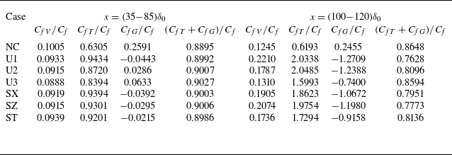
are summarised in table 2.
Relative contributions of terms in the FIK identity to skin friction for
 $A=0.005$
.

Within the blowing region, the viscous term accounts for approximately 10 % of the skin friction, while the Reynolds shear stress term contributes roughly 90 %. The contribution of the mean convection term is negligible in this region. Downstream of the blowing region, the viscous term
 $C_{\!fV}$
constitutes 20 % of the total skin friction. Notably, the Reynolds shear stress term individually exceeds the magnitude of the skin friction itself. However, this excess is compensated by a negative contribution from the mean convection term. Consequently, the combined contribution of the Reynolds shear stress and mean convection terms amounts to 80 % of the skin friction.

 H

 ρ/ρ0
 z=0

 Cf
 Ch
 s
 ρw/ρ0
 A=0.005
 Cfi=0.025FcReθi−1/4

 DR
 x=(35−85)δ0
 x=(100−120)δ0
 DR∝ln(Fm/(ρ0U0)+1)
 DR∝Fm/(ρ0U0)

 x=45δ0
 x=100δ0
 A=0.005
 2.44log(y+)+5.2
 Reτ≈450
 M0=2
 Tw=1.36T0

 DR
 Fm
 Reδ
 Reδ∗=ρ¯wU0δ/μ¯w


 A=0.005
 Lθ
 Lτ
 Lv
 Lp

 x=(35−85)δ0
 Lθ
 Lv
 Lp

 Cf
 CfV
 CfT
 CfG
 CfT+CfG

 ⟨u″⟩c
 y+=20
 Δx+=0

 kzEuv+(kz)
 x=95δ0
 x=85δ0
 x=95δ0
 x=105δ0
 x=115δ0

 x=95δ0
 A=0.005
 A=0.005


