DO PRESIDENTS HAVE MUCH INFLUENCE ON THE ECONOMY?

At first glance, it might seem that presidents have only a minor role in determining the country's economic prosperity. After all, the United States has one of the world's most free-market economic systems, which tends to minimize the role of government. Also, Congress, not the president, controls the budget and holds primary jurisdiction over legislation. Nevertheless, every president since Washington has had congressional allies with whom he has worked to affect economic policy. Certainly, the federal government has a variety of levers by which policy makers can affect the economy. Over time, these policy levers have included taxes, trade policy, land grants and sales, service contracts, procurement programs, regulations, loans, subsidies, antitrust regimes, intellectual property, and even military action. The president has direct control over a subset of these policies. Also, the executive branch can act as a focal point or source of policy, especially when Congress is fractured, gridlocked, or disorganized. And if “animal spirits” play a causal role in national economic performance, as is argued by economists, then the president at his bully pulpit is in a prime position to affect those spirits (Akerlof and Shiller Reference Akerlof and Shiller2009; Wood, Owens, and Durham Reference Wood, Owens and Durham2005). Indeed, the president's effect on the economy can sometimes be powerful. For example, Gauti Eggertsson at the New York Federal Reserve has identified Franklin D. Roosevelt's (FDR) mere inauguration as the turning point of the Great Depression; certainly FDR's subsequent policy agenda was transformational (Eggertsson Reference Eggertsson2008; Brands Reference Brands2008). Therefore, although the executive branch may appear to have a limited role on paper, the historical record suggests that presidents can affect the economy in large ways. Certainly voters seem to think so. Economic issues have been central to almost every presidential election and appear to affect both voter turnout and choice (Evans and Pickup Reference Evans and Pickup2010; Geys Reference Geys2006; Lewis-Beck, Nadeau, and Elias Reference Lewis-Beck, Nadeau and Elias2008; Lewis-Beck and Stegmaier Reference Lewis-Beck and Stegmaier2000; Nadeau and Lewis-Beck Reference Nadeau and Lewis-Beck2001; Singer Reference Singer2011; Vavreck Reference Vavreck2009). Although most scholarly research has focused on this relationship during post-World War II elections, evidence for it has also been found across the history of American elections (Lynch Reference Lynch2002).

If presidents can affect the economy and are judged by voters, historians, and the media by economic outcomes during, or soon after, their administration, then it makes sense to develop more objective ratings of presidential economic performance.

WHICH DATA WAS USED AND WHY

Which data should be used to judge presidential economic performance? There is simply no objective answer to this question. Even experts disagree on precisely which indicators to include and how to weight these. Research has further shown that perceptions of performance and responsibility can be affected by partisanship (Tilley and Hobolt Reference Tilley and Hobolt2011; Uscinski and Simon Reference Uscinski and Simon2011). This applies not only to scope conditions, but also which data to include, weights to assign, and algorithms to use. This problem is exacerbated by the fact that, clearly, initial choices about data and weights will affect the results. For example, in one ranking exercise, the libertarian Von Mises Institute uses only government spending as a percent of total output (Vedder and Gallaway Reference Vedder and Gallaway2001). Naturally, wartime big-spenders (e.g., Lincoln, Wilson, and FDR) rank near the bottom of that list, while their successors, all peacetime budget-slashers, came in on top (e.g., A Johnson, Harding, and Truman). Conversely, we can assume that a left-leaning judge might instead select measures such as income inequality, welfare spending, or poverty levels, and wind up placing some of those same big-spender presidents among the top ranks.

To minimize partisan or ideological subjectivity, this article includes those indicators that are most often mentioned by mainstream Western economists, the media, and voters when judging US economic performance. After all, to judge American presidents using mainstream American economic values makes sense. This approach does not eliminate subjectivity, but it should remove personal political biases from the equation. It also attempts to match the ranking criteria with popular preferences. That is, it puts the American public at the judge's table, rather than some supposedly “objective” expert or group.

First, mainstream economists, policymakers, and observers generally applaud an economy that simultaneously achieves four goals:

• • increases national wealth

• • reduces unemployment

• • minimizes inflation

• • reduces the balance of payments burden

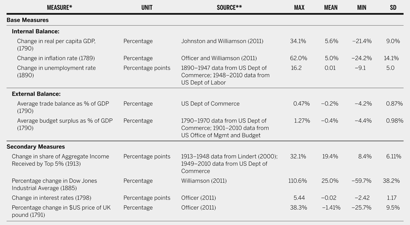
Here, this combination of indicators is used as the base measure of economic performance. To construct the rankings, four more indicators are added: reduction in economic inequality, currency strength, interest rate changes, and stock market performance. These additional indicators are included because (1) they are also generally viewed as broad measures of macroeconomic performance, (2) reliable data exist over long periods of time, and (3) they do not correlate highly with each other or with the base indicators; therefore they likely capture different aspects of economic performance. Data with these characteristics are rare. Also, critics might argue that the four base measures are insufficient data on which to base presidential rankings. Therefore, these secondary measures bring valuable scope and depth to the calculation. The description of these data and summary statistics are abstracted in table 1. Complete explanations of the data sources, coding rules, and selection criteria are available in the online appendices at www.mzak.net.

Table 1

Data Description

* First year of time series indicated in parentheses.

** See appendix I for full citations.

Although every effort has been made to minimize error and subjective judgments in the economic rankings previously reported, two inherent biases are worth pointing out. First, the choices of measures and weightings do contain assumptions in favor of mainstream neoclassical, perhaps neo-Keynesian, economics as is taught in most American universities (e.g., Mankiw Reference Mankiw2011). Therefore, although measures of unemployment and income inequality are included in the rankings, the overall weightings tend to favor the achievement of wealth and efficiency over economic equity or social justice. Although it makes sense to judge American executives using mainstream American economic values, this does not make these values objectively correct. Second, all economic data suffers from statistical errors and heteroskedasticity issues that increase as these time series recede back in time. This ranking exercise is no different. Even with modern data gathering apparatus, most of the economic indicators used are difficult to calculate; indeed, historical estimates are even more fraught with statistical error.

This study addresses these weaknesses in three ways. First, the rating system used here communicates in an accurate and familiar way the “signal” contained in the economic data, while simultaneously being explicit about the “noise” and subjective judgments involved in this type of exercise. It also attempts to correct for noise and bias by using triangulation, four-year periods, multiple time lags, and competing ranking algorithms. That is, the economic data, while containing error bars, does communicate objective information about economic performance that this study isolates. Second, the aggregation of data into four-year periods helps eliminate some of the problems involved in making point estimates for individual years, as well as average out some of the random error. In those cases where change over time is measured, as long as the error is similar across each year (either random or systematic), it will tend to be subtracted out. Finally, all data are available for other scholars, using their own scoring rules, weights, and additional input measures (e.g., leadership, progress in science and technology, wealth redistribution) to construct their own rankings for comparison.

HOW THE GRADES WERE CALCULATED

Grades were assigned similarly to that of professors evaluating their students. Each student (presidential administration) is given eight assignments (the eight indicators of national wealth, inflation, employment, etc.). Performance on these assignments is graded individually using a traditional A–F (4–0 point) grading scale that is curved, as discussed later. Then, those grades are averaged into an overall GPA and class ranking. In calculating the grades and GPAs, each of the economic indicators was weighted equally and intuitively graded. The use of grades and GPAs is not intended to be cavalier, flippant, or cute. These are advantageous in several ways. First, grades constitute a ranking system that is accessible and familiar to most readers. Second, grades most explicitly and honestly reflect the strengths and weaknesses of a rating exercise such as this. As teachers, parents, and former students, most readers will recognize that, like grades received in school, the grades reported here are an approximation. Grades are never perfect measures, but they are often good indicators of performance.

To provide a pragmatic and credible ranking of the presidents, several techniques drive down random error and systematic bias. For example, because there is no consensus as to precisely when a new president becomes responsible for the economy, the GPAs were calculated separately for honeymoon periods of zero, one, and two years. Also, two competing grade curves were used. The first algorithm used strict quintiles: the top 20% of performers received an “A” (4 points), the second 20% received a “B” (3 points), and so forth. The second algorithm imposed a bell-curve. Specifically a “C” (2 points) was awarded to all scores within one standard deviation of the mean, centered on the mean. For the next half standard deviation, a “B” or “D” was awarded as appropriate; for the remaining administrations, an “A” or “F” was awarded accordingly. This method rewards or punishes extremes in performance to better identify truly great or poor executives while expanding the number of administrations considered to be merely average. After the individual indicators were graded, these were combined via a simple average into an overall grade for each administration or president.

The final GPA calculation brought together all of the above grades to produce tables 2 and 3. For each president, each final “strict quintile” and “bell-curve” GPA for each honeymoon period was averaged together and a final GPA assigned. Thus, to earn a 3.00 or higher, a president or administration had to consistently score well, regardless of honeymoon period or grading algorithm (e.g., FDR consistently got As throughout each different scoring approach). Likewise, to earn a GPA below 1.00, a president or administration had to consistently and robustly perform poorly.

Table 2

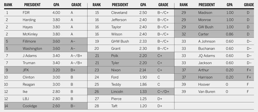
Economic Grades and Rankings of the Presidents

Notes: Average GPA = 2.04, Standard Deviation = 1.21, Max/Min = 4/0.

The following shortened forms of presidents names are as follows: J Adams = John Adam: JQ Adams = John Quincy Adams; Ike = Dwight D. Eisenhower, GHW Bush = George Herbert Walker Bush; GW Bush = George W. Bush; A Johnson = Andrew Johnson; LBJ = Lyndon Baines Johnson; Teddy = Theodore Roosevelt; FDR = Franklin Delano Roosevelt; JFK = John F. Kennedy.

Table 3

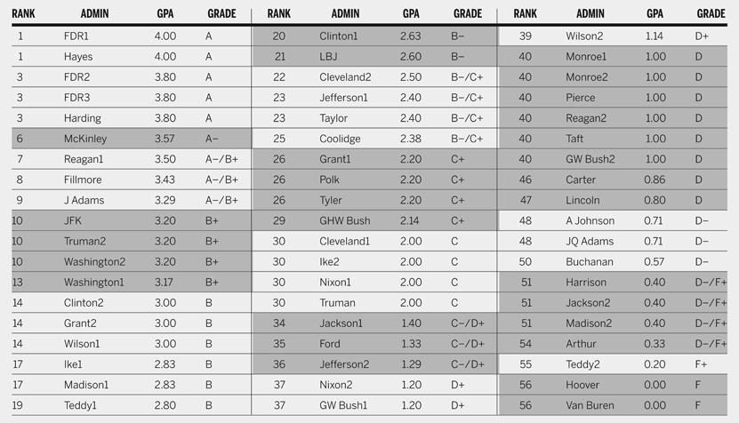
Economic Grades and Rankings of the Administrations*

Notes: Average GPA = 2.00, Standard Deviation = 1.18, Max/Min = 4/0.

* See online appendices for an explanation of the codings of irregular administrations.

A complete explanation of the grading methodology, as well as resolutions of technical issues, is available in the online appendices (at www.mzak.net). There, readers can find technical discussions of issues such as periodization, multicollinearity, cross-algorithm consistency, and data commensurability. Each of these issues was addressed with the goal of minimizing bias and error. Perhaps more importantly, all data used in these rankings are publicly available for readers who prefer to replicate or critique my methods, or to calculate alternative rankings using their own scoring rules, weights, or additional input data. Interested scholars might further address particular presidents who they find to be controversial using historical research or more in-depth statistical methods.

ECONOMIC GPAS AND RANKINGS, 1789–2009

Tables 2 and 3 report the results of this novel rating system of presidential economic performance based solely on quantitative data and generated by the methods described in the Appendices. The first set of ratings awards each president an economic GPA and relative ranking (table 2). The second set awards each separate administration a GPA and relative ranking (table 3). A casual examination of the tables reveals some surprises, such as the high rankings of some traditionally poorly regarded presidents (e.g., Harding, Hayes, and Fillmore) or the relatively low rankings of some national heroes (e.g., Lincoln, Madison, Monroe, JQ Adams, and Jackson). These apparent paradoxes are resolved in the subsequent text. Analysis of the grades and their correlations with other measures (party, veto-players, partisanship, presidential background) are also discussed.

It is tempting to dismiss these rankings as the product of dumb luck: getting elected at the top or bottom of the business cycle. Randomness surely plays some role in these rankings but, as argued previously, presidents also bear responsibility for making their own luck. For example, Van Buren and Hoover did not receive the lowest grades merely by accident of the major economic depressions that struck during their presidencies. For decades before the Panics of 1837 and 1839, Martin Van Buren and his Democratic party eviscerated the very institutions that could have ameliorated the Depression of 1839–1843 that ruined his presidency. Nearly a century later, Republican Herbert Hoover took relatively minor actions in response to the Great Depression, adhering instead to the classical economic beliefs of his time that markets would self-correct and that the federal government had no business providing aid or welfare to individuals. Meanwhile neither Hayes nor FDR simply “lucked out” by entering office near the bottom of a depression. Hayes was an intelligent, adroit administrator who played physician to the plague of scandals and ineptitudes afflicting the preceding Grant administration. Hayes actively attacked corruption, reduced the national debt, restored public credit, and forcefully addressed the new phenomenon of militant labor strikes. Decades later, FDR set unique precedents for government intervention in the economy in his attempts to end the Great Depression. More historical analysis is needed to better resolve the responsibility of each president for his economic performance. Generally speaking, however, this article contends that presidents are neither helpless victims nor lucky lottery winners; hence their economic GPAs should not be dismissed as random draws.

HYPOTHESES

The economic performance GPAs allow us to test for general correlations and thereby generate hypotheses about the relationship between the president and the economy. The variables considered below include political party type, federal veto players, partisanship, war, economic class origins, intelligence and open-mindedness, prepolitical career, birth order, historical greatness, and dark horse versus well-vetted presidents. Notably, this article does not analyze the effects of economic performance on elections, which is covered elsewhere by a vast scholarly literature (Evans and Pickup Reference Evans and Pickup2010; Geys Reference Geys2006; Lewis-Beck, Nadeau, and Elias Reference Lewis-Beck, Nadeau and Elias2008; Lewis-Beck and Stegmaier Reference Lewis-Beck and Stegmaier2000; Nadeau and Lewis-Beck Reference Nadeau and Lewis-Beck2001; Singer Reference Singer2011; Vavreck Reference Vavreck2009). Because correlations cannot show causal mechanism, and do not control for conditional variables, this is a hypothesis generation exercise intended to motivate further research. Each of these observations is also robust to whether only the base data were used (per capita GDP, inflation, balance of payments) or the overall dataset (which includes unemployment, stock market, interest rates, inequality, and currency strength).

WHAT'S THE POINT?

Some readers might be tempted to dismiss this exercise as a bit of intellectual fun with numbers, they should not be so hasty. The economic rankings reported here are not intended to create the impossible (e.g., a perfectly unbiased and error-free ranking of the presidents). Rather, the objective is to eliminate bias and statistical error where possible and to be transparent about that which might remain. If one goal of science is to advance empirical measures through experimentation, then the data-based rankings presented in this article are meant seriously as a step in this evolution.

More importantly, scholars should not err in letting the perfect (or near perfect) be the enemy of the good that these rankings can do: to provoke constructive debate about presidential performance and responsibility. For example, these rankings highlight the fact that even nonpartisan, nonideological decisions about scope and historical context have a subjective component that can affect performance metrics. Economic performance is the product of a multitude of forces and actors. The effects of some of these variables may not be realized for decades. Therefore, any ultimate judgment on an individual president depends on the judge's scope conditions. Thus, it is important for rankings, and their advocates, to be clear about their subjective aspects rather than advance the pretense of objectivity. Because such naïve candidness will likely be infrequent, it is imperative that scholars enter this debate to identify and publicize the nonscientific or biased aspects of agenda-driven rankings.

Another goal of this article is to show that scientific analysis of economic data can be a useful step toward a more objective consensus. Despite the problems with subjectivity, scholars and voters need to thoughtfully debate how much any particular president is responsible for the economy on his watch relative to other actors. Different degrees of institutional responsibility have existed across history. Some scholars argue further that the president's economic advisers can also make an substantial impact on policy, and, hence, performance (Goff Reference Goff2010). Furthermore, ethical judgments need to be made about how to divvy up responsibility between actors, institutions, and environment. Again, all of these have subjective components that can vary across different observers.

The rankings presented here demonstrate one way to approach these problems. Readers are encouraged to dig deeper into history, gather data, try their own rankings, and perhaps use them to consider how they view (and vote for) the president. Put simply, if “it's the economy, stupid,” then we need to make stronger efforts to properly judge economic performance and to assign credit and blame where they are most deserved. These rankings are meant to constitute a scientific step in this direction.

ACKNOWLEDGMENTS

For their help with data, methodology, editing, and framing, much thanks to Peter Brecke, David Campbell, Chris J. Dolan, John Frendreis, James K. Galbraith, Jeffrey Isaac, Gregory Burr Lewis, Peter Lindert, Emmanuel Saez, Ken Sherrill, Raymond Tatalovich, Sean Twombly, Joseph E. Uscinski, Dan Winship, and Scott Winship.