
I. INTRODUCTION
Dynamic recrystallization (DRX) is one of most important microstructural evolution mechanisms for most of metals and alloys during hot deformation, such as forging. During DRX, the initial coarse-grains are gradually replaced by fine DRX grains. The final microstructures of forgings greatly depend on the DRX volume fraction and grain size. Reference McQueen1,Reference De Jaeger, Solas, Fandeur, Schmitt and Rey2 Incomplete DRX, where the DRX volume fraction is less than 95%, will result in serious mixed structures with fine and coarse grains. This is not permitted or expected since the mixed structure will seriously deteriorate the mechanical properties for most materials. Therefore, it is very significant to precisely predict and control the DRX volume fraction of forgings after hot deformation.
The DRX kinetics model is essential to predict and control the DRX volume fraction of forgings. In recent decades, some efforts have been made to investigate the DRX behaviors and kinetics models of various metals and alloys, such as Nb-steels, Reference Beladi and Hodgson3,Reference Vervynckt, Verbeken, Thibaux and Houbaert4 Aermet100 steel, Reference Ji, Li, Li, Li and Li5 38MnVS6 Steel, Reference Gu, Zhang, Zhang, Ruan and Zhen6 42CrMo steel, Reference Chen, Lin and Ma7 a low carbon vanadium-nitride microalloyed steel, Reference Zhao, Zhao, Li and Lu8 SCM435 steel, Reference Xu, Zhu, Tang and Sun9 300M steel, Reference Liu, Li and Luo10 17-4 PH stainless steel, Reference Mirzadeh and Najafizadeh11 X70 pipeline steel, Reference Xu, Tang, Song and Pan12 titanium-modified austenitic stainless steel, Reference Mandal, Sivaprasad and Dube13 410 martensitic stainless steel, Reference Momeni and Dehghani14 superaustenitic stainless steel, Reference Ebrahimi, Keshmiri, Momeni and Mazinani15 304 stainless steel, Reference Stewart, Jonas and Montheillet16–Reference Ohadi, Parsa and Mirzadeh18 martensitic stainless steel, Reference Ebrahimi, Keshmiri, Maldad and Momeni19 high purity and ultra-high purity austenitic stainless steels, Reference El Wahabi, Gavard, Montheillet, Cabrera and Prado20 Cu-0.4 Mg alloy, Reference Ji, Li and Li21 magnesium alloys, Reference Changizian, Zarei-Hanzaki and Abedi22 Mg–Y–Nd–Zr alloy, Reference Zhang, Yang, Sun, Li, Wang, Zhang, Ye and Sakai23 Mg–Li–Al–Nd duplex alloy, Reference Xu, Peng, Qin, Chen, Yang and Wei24 Mg–Gd–Y–Zr alloy, Reference Xiao, Jiang, Tang, Hao, Gao, Chen and Liu25 Mg–2.0Zn–0.3Zr alloy, Reference Lv, Peng, Shi, Tang and Pan26 TiAl alloy, Reference Cui, Kong, Wang, Chen and Zhou27 Ti55511 titanium alloy, Reference Tan, Li, Guan, Yang and Shu28 FGH4096 superalloy, Reference Ning, Yao, Fu and Guo29 and typical Ni-based superalloys. Reference Zhang, Zhang, Zhou, Lu, Zhao and Yang30–Reference Chen, Lin, Li and Zhou34 In these works, hot compressive or tensile tests with constant deformation temperature and strain rate were usually used to investigate the effects of thermomechanical parameters (temperature, strain rate, and strain), chemical compositions, Reference Beladi and Hodgson3 initial grain size, Reference Chen, Lin and Ma7,Reference Ohadi, Parsa and Mirzadeh18,Reference El Wahabi, Gavard, Montheillet, Cabrera and Prado20 and precipitates Reference Vervynckt, Verbeken, Thibaux and Houbaert4,Reference Changizian, Zarei-Hanzaki and Abedi22,Reference Lin, He, Chen, Chen, Zhao, Ma and Long33,Reference Riedel and Svoboda35–Reference Hallberg, Svendsen, Kayser and Ristinmaa37 on DRX behaviors. The DRX volume fractions of materials were often evaluated by analyzing true stress-true strain curves. Reference Tan, Li, Guan, Yang and Shu28,Reference Mejía, Bedolla-Jacuinde, Maldonado and Cabrera38,Reference Quan, Pu, Wen, Zou and Zhou39 It was found that the dependence of DRX volume fraction on strain under constant deformation temperature and strain rate can be described by the Avrami equation. Reference Jonas, Quelennec, Jiang and Martin40 Therefore, the Avrami equation is often applied to describe the DRX kinetics behavior. εc (the critical strain for the onset of DRX), ε0.5 (the strain for 50% DRX), εp (the strain for peak stress), and ε* (the strain for maximum softening rate) are the characteristic parameters of kinetics models. The characteristic parameters are often expressed as the functions of deformation temperature and strain rate Reference Chen, Lin, Li and Zhou34 or Zener–Hollomon parameter. Reference Zhao, Zhao, Li and Lu8,Reference Xu, Tang, Song and Pan12,Reference Ebrahimi, Keshmiri, Maldad and Momeni19,Reference Ji, Li and Li21,Reference Xu, Peng, Qin, Chen, Yang and Wei24,Reference Chen, Lin, Wen, Zhang and He31 For some researches, Reference Chen, Lin and Ma7,Reference Liu, Li and Luo10,Reference Ohadi, Parsa and Mirzadeh18,Reference El Wahabi, Gavard, Montheillet, Cabrera and Prado20 the effect of initial grain size on DRX behaviors was considered. Thus, the characteristic parameters are also expressed as the functions of initial grain size, deformation temperature and strain rate. Besides the Avrami equation, Liu et al. Reference Liu, Cui and Ruan41 proposed a new DRX kinetics model which can represent the ‘slow–rapid–slow’ property of DRX development. It is well known that the classical DRX kinetics models can be expediently used to predict the DRX volume fractions under constant deformation temperature and strain rate, because the characteristic parameters, such as εc, εp, ε0.5, and ε*, remain constant. However, the real deformation temperature and strain rate of metals and alloys during hot deformation are often time-varying. Reference Won Lee and Im42 So, it is very important to evaluate the DRX volume fractions under inconstant deformation temperature and strain rate. But, there will be a question when the classical DRX kinetics models are applied to evaluate the DRX volume fractions under inconstant deformation temperature and strain rate. i.e., the characteristic parameters (εc, εp, ε0.5, and ε*) should be calculated by which deformation temperature and strain rate? Obviously, the classic DRX kinetics models cannot be directly applied in inconstant deformation temperature and strain rate conditions. Therefore, the classic DRX kinetics models need to be improved.
In this study, an improved DRX kinetics model, which can well describe the DRX kinetics under inconstant deformation temperature and strain rate conditions, is proposed. The proposition of improved model is based on the hypothesis that the derivatives of DRX volume fraction with respect to strain only depends on the current deformation temperature, strain rate, and DRX volume fraction. To verify the improved model, the hot compressive tests under the variant strain rate were carried out on a typical solution-treated Ni-based superalloy.
II. THE PROPOSITION OF AN IMPROVED DRX KINETICS MODEL
A. Classical DRX kinetics models
The general form of classical DRX kinetics models can be expressed as:
 $${X_{{\rm{drx}}}} = 1 - \exp \left[ { - k{{\left( {{{\varepsilon - {\varepsilon _{\rm{c}}}} \over {\varepsilon '}}} \right)}^n}} \right]\quad ,$$
where ε is the strain, X drx is the DRX volume fraction at the strain of ε, εc is the critical strain for the onset of DRX, ε′ can be a particular strain such as ε* (the strain for maximum softening rate), Reference Lv, Peng, Shi, Tang and Pan26,Reference Xu, Hu and Sun43–Reference Jia, Zhang and Lu45 εp (the strain for peak stress), Reference Zhao, Zhao, Li and Lu8,Reference Liu, Li and Luo10,Reference Wei, Liu, Xiao and Zhang46 εc (the critical strain for the onset of DRX), Reference Ji, Li, Li, Li and Li5,Reference Ji, Li and Li21 and (ε0.5 − εc), Reference Chen, Lin and Ma7,Reference Chen, Lin, Wen, Zhang and He31,Reference Chen, Lin, Li and Zhou34 n is the material constant (Avrami exponent) related to the DRX nucleation mechanism, and k is a constant related to ε′ or materials.
When ε′ is (ε0.5 − εc), the value of
 $k$
is 0.693 (or −ln 0.5). i.e., Eq. (1) can be changed as:
 $${X_{{\rm{drx}}}} = 1 - \exp \left[ { - 0.693{{\left( {{{\varepsilon - {\varepsilon _{\rm{c}}}} \over {{\varepsilon _{0.5}} - {\varepsilon _{\rm{c}}}}}} \right)}^n}} \right]\quad .$$
For some metals and alloys, (ε0.5 − εc) is usually replaced by ε0.5 since ε0.5 is often much larger than εc. i.e., the following equation is also widely used to describe the DRX kinetics. Reference Cheng, Chang, Tang, Kou and Li47–Reference Li, Duan, Li and Wu49
 $${X_{{\rm{drx}}}} = 1 - \exp \left[ { - 0.693{{\left( {{{\varepsilon - {\varepsilon _{\rm{c}}}} \over {{\varepsilon _{0.5}}}}} \right)}^n}} \right]\quad .$$
Usually, εc and ε0.5 can be expressed as the functions of deformation temperature (T, unit: K) and strain rate (
 $\dot \varepsilon$
, unit: s−1).
Reference Chen, Lin, Li and Zhou34
 $$\left\{ \matrix{ {\varepsilon _{\rm{c}}} = {a_1}{{\dot \varepsilon }^{{m_1}}}\,\exp \left( {{{{Q_1}} \mathord{\left/ {\vphantom {{{Q_1}} T}} \right. \kern-\nulldelimiterspace} T}} \right) \hfill \cr {\varepsilon _{0.5}} = {a_2}{{\dot \varepsilon }^{{m_2}}}\,\exp \left( {{{{Q_2}} \mathord{\left/ {\vphantom {{{Q_2}} T}} \right. \kern-\nulldelimiterspace} T}} \right) \hfill \cr} \right.$$
in which a 1, a 2, m 1, m 2, Q 1, and Q 2 are material constants. εc and ε0.5 can also be expressed as the functions of Zener–Hollomon parameter (Z).
 $$\left\{ \matrix{ {\varepsilon _{\rm{c}}} = {a_1}{Z^{{m_1}}} \hfill \cr {\varepsilon _{0.5}} = {a_2}{Z^{{m_2}}} \hfill \cr Z = \dot \varepsilon \,\exp \left[ {{Q \mathord{\left/ {\vphantom {Q {\left( {RT} \right)}}} \right. \kern-\nulldelimiterspace} {\left( {RT} \right)}}} \right] \hfill \cr} \right.$$
in which Q is the deformation activation energy (J/mol) and R is the universal gas constant [8.314 J/(mol K)].
When ε′ = ε* or ε′ = εp, the value of k should be obtained by the linear regression to experimental data.
Reference Xu, Hu and Sun43–Reference Jia, Zhang and Lu45
Therefore, the value of k is related to materials. ε* and εp can also expressed as the functions of T and
 $\dot \varepsilon$
or Z.
 $$\left\{ \matrix{ {\varepsilon ^ * } = {a_3}{{\dot \varepsilon }^{{m_3}}}\,\exp \left( {{{{Q_3}} \mathord{\left/ {\vphantom {{{Q_3}} T}} \right. \kern-\nulldelimiterspace} T}} \right) \hfill \cr {\varepsilon _{\rm{p}}} = {a_4}{{\dot \varepsilon }^{{m_4}}}\,\exp \left( {{{{Q_4}} \mathord{\left/ {\vphantom {{{Q_4}} T}} \right. \kern-\nulldelimiterspace} T}} \right) \hfill \cr} \right.$$
 $$\left\{ \matrix{ {\varepsilon ^ * } = {a_3}{Z^{{m_3}}} \hfill \cr {\varepsilon _{\rm{p}}} = {a_4}{Z^{{m_4}}} \hfill \cr} \right.$$
in which a
3, a
4, m
3, m
4, Q
3, and Q
4 are material constants. If the effect of initial grain size (d
0) on DRX kinetics behavior is considered, εc, εp, ε0.5, and ε* will be expressed as the function of d
0, T, and
 $\dot \varepsilon$
.
Reference Chen, Lin and Ma7
For a given constant T and
 $\dot \varepsilon$
, the values of εc and ε′ are constants and can be determined by Eqs. (4)–(7). Therefore, the values of X
drx at arbitrary strain can be directly obtained by Eq. (1). However, for inconstant T and
 $\dot \varepsilon$
, the values of εc and ε′ cannot be obtained by Eqs. (4)–(7) because the value of Zener–Hollomon parameter is time-varying. Thus, the values of X
drx at arbitrary strain cannot be evaluated by classic DRX kinetics models. So, the classic DRX kinetics models need to be improved.
B. An improved DRX kinetics model
For predicting the DRX volume fraction under inconstant T and
 $\dot \varepsilon$
, it is natural to obtain the derivative of DRX volume fraction with respect to strain νdrx(ε) firstly. That is,
 $${\nu _{{\rm{drx}}}}\left( \varepsilon \right) = {{{\rm{d}}{X_{{\rm{drx}}}}} \over {{\rm{d}}\varepsilon }} = {{\partial {X_{{\rm{drx}}}}} \over {\partial \varepsilon }} + {{\partial {X_{{\rm{drx}}}}} \over {\partial T}}{{{\rm{d}}T\left( \varepsilon \right)} \over {{\rm{d}}\varepsilon }} + {{\partial {X_{{\rm{drx}}}}} \over {\partial \dot \varepsilon }}{{{\rm{d}}\dot \varepsilon \left( \varepsilon \right)} \over {{\rm{d}}\varepsilon }}$$
in which T(ε) is the temperature function of strain, and
 $\dot \varepsilon \left( \varepsilon \right)$
is the strain rate function of strain.
Then, the value of X drx can be obtained by:
 $${X_{{\rm{drx}}}} = \int_0^\varepsilon {{{{\rm{d}}{X_{{\rm{drx}}}}} \over {{\rm{d}}\varepsilon }}{\rm{d}}\varepsilon } = \int_0^\varepsilon {{\nu _{{\rm{drx}}}}\left( \varepsilon \right)\,{\rm{d}}\varepsilon } \quad .$$
However, T(ε) and
 $\dot \varepsilon \left( \varepsilon \right)$
are likely nondifferential for the practical hot deformation. That is, dT(ε)/dε and
 ${{{\rm{d}}\dot \varepsilon \left( \varepsilon \right)} \mathord{\left/ {\vphantom {{{\rm{d}}\dot \varepsilon \left( \varepsilon \right)} {{\rm{d}}\varepsilon }}} \right. \kern-\nulldelimiterspace} {{\rm{d}}\varepsilon }}$
often do not exist. It is hard to obtain the explicit expression of νdrx(ε) or the value of νdrx(ε) at a given strain. Therefore, it is almost impossible to obtain the value of X
drx by Eqs. (8) and (9) in the practical hot deformation.
In the study, an improved DRX kinetics model is proposed based on the hypothesis that the value of νdrx(ε) only depends on the current T,
 $\dot \varepsilon$
and X
drx. Namely, the effects of dT(ε)/dε and
 ${{{\rm{d}}\dot \varepsilon \left( \varepsilon \right)} \mathord{\left/ {\vphantom {{{\rm{d}}\dot \varepsilon \left( \varepsilon \right)} {{\rm{d}}\varepsilon }}} \right. \kern-\nulldelimiterspace} {{\rm{d}}\varepsilon }}$
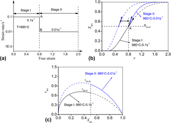
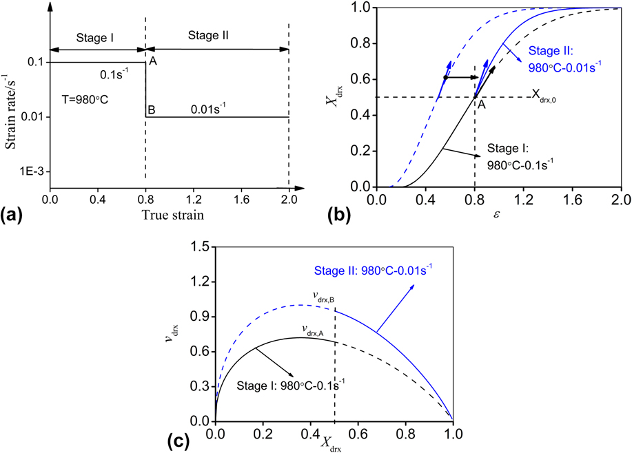
on DRX are neglected. The hypothesis can be explained by an example shown in Fig. 1. The material is assumed to be deformed with two stages, as shown in Fig. 1(a). In stage I, T and
 $\dot \varepsilon$
remain constant (980 °C and 0.1 s−1). Therefore, the variation of X
drx with ε can be evaluated by classical DRX kinetics models, as shown Fig. 1(b). In stage I, the value of νdrx(ε) can be evaluated by Eq. (10) because dT(ε)/dε and
 ${{{\rm{d}}\dot \varepsilon \left( \varepsilon \right)} \mathord{\left/ {\vphantom {{{\rm{d}}\dot \varepsilon \left( \varepsilon \right)} {{\rm{d}}\varepsilon }}} \right. \kern-\nulldelimiterspace} {{\rm{d}}\varepsilon }}$
are equal to zero:
 $$\left\{ \matrix{ {\nu _{{\rm{drx}}}}\left( \varepsilon \right) = {{{\rm{d}}{X_{{\rm{drx}}}}} \over {{\rm{d}}\varepsilon }} = {{\partial {X_{{\rm{drx}}}}} \over {\partial \varepsilon }} = {{nk} \over {\varepsilon '}}\left( {1 - {X_{{\rm{drx}}}}} \right){\left[ { - {1 \over k}{\rm{In}}\left( {1 - {X_{{\rm{drx}}}}} \right)} \right]^{{{n - 1} \over n}}} \hfill \cr \varepsilon ' = f\left( {T = 980\,^\circ {\rm{C,}}\;\dot \varepsilon = 0.01\,{{\rm{s}}^{ - 1}}{\rm{\ }}} \right) \hfill \cr} \right.\quad {\rm{when}}\;{X_{{\rm{drx}}}} > 0$$
in which X
drx at given ε can be evaluated by classical DRX kinetics models, such as Eq. (2). ε′ can be determined by the current T (980 °C) and
 $\dot \varepsilon$
(0.1 s−1). The change of νdrx with X
drx in stage I is shown in Fig. 1(c). At the end of stage I (just before the change of strain rate, Point A), νdrx,A (the value of νdrx at point A) can be evaluated by:
 $$\left\{ \matrix{ {\nu _{{\rm{drx,A}}}} = {{nk} \over {\varepsilon '}}\left( {1 - {X_{{\rm{drx,0}}}}} \right){\left[ { - {1 \over k}\ln \left( {1 - {X_{{\rm{drx,0}}}}} \right)} \right]^{{{n - 1} \over n}}} \hfill \cr \varepsilon ' = f\left( {T = 980\,^\circ {\rm{C,}}\;\dot \varepsilon = 0.01\,{{\rm{s}}^{ - 1}}{\rm{\ }}} \right) \hfill \cr} \right.$$
in which X
drx,0 is the value of X
drx at the end of stage I. When the strain rate is abruptly decreased to 0.001 s−1 at the start of stage II [Point B, as show in Fig. 1(a)], the value of νdrx will be also abruptly changed. If the effects of dT(ε)/dε and
 ${\rm{d}}\dot \varepsilon \left( \varepsilon \right)/{\rm{d}}\varepsilon$
on DRX are neglected, the value of νdrx at the start of stage II (νdrx,B) can be evaluated by:
 $$\left\{ \matrix{ {\nu _{{\rm{drx,B}}}} = {{nk} \over {\varepsilon '}}\left( {1 - {X_{{\rm{drx,0}}}}} \right){\left[ { - {1 \over k}\ln \left( {1 - {X_{{\rm{drx,0}}}}} \right)} \right]^{{{n - 1} \over n}}} \hfill \cr \varepsilon ' = f\left( {T = 980\,^\circ {\rm{C}},\;\dot \varepsilon = 0.001\,{{\rm{s}}^{ - 1}}{\rm{\ }}} \right) \hfill \cr} \right.\quad ,$$
where X drx,0 is also the value of X drx at the start of stage II.
Schematic diagrams of the hypothesis that the value of νdrx(ε) only depends on the current T,
 $\dot \varepsilon$
and X
drx: (a) variation of
 $\dot \varepsilon$
with ε; (b) variation of X
drx with ε; (c) variation of νdrx with X
drx.
Therefore, an improved DRX kinetics model can be proposed according to the above hypothesis:
 $${\nu _{{\rm{drx}}}}\left( {T,\dot \varepsilon ,{X_{{\rm{drx}}}}} \right) =\; {{nk} \over {\varepsilon '}}\left( {1 - {X_{{\rm{drx}}}}} \right){\left[ { - {1 \over k}\ln \left( {1 - {X_{{\rm{drx}}}}} \right)} \right]^{{{n - 1} \over n}}}\quad {\rm{when}}\;{X_{{\rm{drx}}}} > 0\quad ,$$
where ε′ is determined by the current T and
 $\dot \varepsilon$
, and can be evaluated by Eqs. (4)–(7).
If ε′ = ε0.5 − εc, Eq. (13) can be changed as:
 $$\left\{ \matrix{ {\nu _{{\rm{drx}}}}(T,\dot \varepsilon ,{X_{{\rm{drx}}}}) = {{nk} \over {{\varepsilon _{0.5}} - {\varepsilon _{\rm{c}}}}}\left( {1 - {X_{{\rm{drx}}}}} \right){\left[ { - {1 \over k}\ln \left( {1 - {X_{{\rm{drx}}}}} \right)} \right]^{{{n - 1} \over n}}} \hfill \cr \hfill \cr {\varepsilon _{\rm{c}}} = {a_1}{{\dot \varepsilon }^{{m_1}}}\,\exp \left[ {{{{Q_1}} \mathord{\left/ {\vphantom {{{Q_1}} T}} \right. \kern-\nulldelimiterspace} T}} \right] \hfill \cr {\varepsilon _{0.5}} = {a_2}{{\dot \varepsilon }^{{m_2}}}\,\exp \left[ {{{{Q_2}} \mathord{\left/ {\vphantom {{{Q_2}} T}} \right. \kern-\nulldelimiterspace} T}} \right] \hfill \cr} \right.\quad {\rm{when}}\;{X_{{\rm{drx}}}} > 0$$
in which k is 0.693.
Under inconstant T and
 $\dot \varepsilon$
, the value of X
drx can be evaluated by numerical integration methods, such as rectangle rule.
 $${X_{{\rm{drx}},l}} = \sum\limits_{i = 1}^{l - 1} {{{\left( {{{{\rm{d}}{X_{{\rm{drx}}}}} \over {{\rm{d}}\varepsilon }}} \right)}_i}\left( {{\varepsilon _i} - {\varepsilon _{i - 1}}} \right)} = \sum\limits_{i = 1}^{l - 1} {{\nu _{{\rm{drx}},i}}\left( {{\varepsilon _i} - {\varepsilon _{i - 1}}} \right)}$$
in which X drx,l is the value of X drx at the strain of ε l , νdrx,i is the value of dX drx/dε at the strain ε i . If Δε (= ε i − ε i−1) is enough small, the value of X drx,l obtained by Eq. (15) will be very close to the true one.
III. EXPERIMENTAL VERIFICATION OF THE IMPROVED DRX KINETICS MODEL
To verify the above improved DRX kinetics model, hot compressive tests with the inconstant strain rate were firstly done on a solution-treated Ni-based superalloy. Secondly, the DRX volume fractions of deformed specimens were obtained by analyzing optical micrographs. Finally, the comparisons between the experimental DRX volume fractions and those predicted by the improved DRX kinetics model were carried out.
A. Materials and experiments
The experimental material is a typical Ni-based superalloy with the composition (wt%) of 52.82Ni–18.96Cr–5.23Nb–3.01Mo–1.00Ti–0.59Al–0.01Co–0.03C–(bal.) Fe. Cylindrical specimens of
 $\phi 10\,{\rm{mm}} \times 12\,{\rm{mm}}$
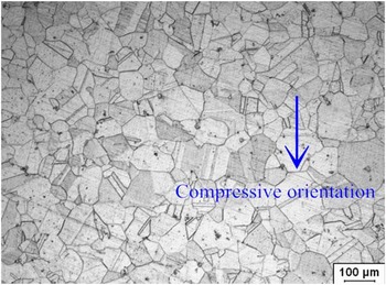
were machined from a forged billet. Before hot compressive tests, all specimens were solution-treated at 1040 °C for 45 min in heat treatment furnace, then quenched by water. Figure 2 shows the starting optical microstructure of the solution-treated superalloy. The average grain size of material is about 75 µm.
Reference Chen, Lin, Li and Zhou34
The starting optical microstructure of the solution-treated superalloy.

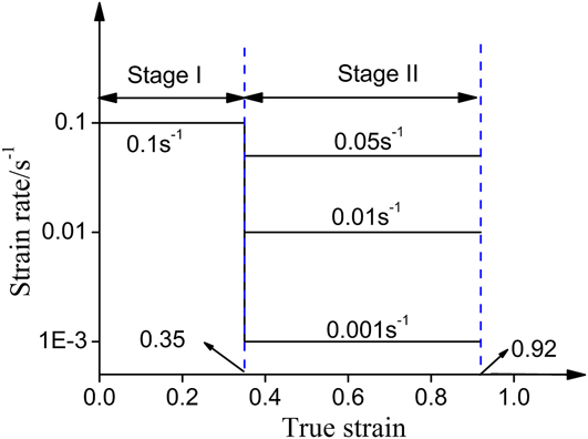
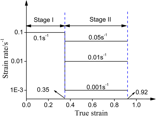
The experimental scheme of hot compressive tests is shown in Fig. 3. The compressive process includes two stages: I and II. The specimens were firstly compressed at the strain rate of 0.1 s−1 to the true strain of 0.35 (height reduction is 30%). Then, the strain rate was immediately dropped to low values (0.001, 0.01, or 0.05 s−1), and the specimens continued to be compressed to the true strain of 0.92 (total height reduction is 60%). For the convenience of elaboration, the above three different inconstant strain rate cases are represented by “0.1–0.001 s−1”, “0.1–0.01 s−1”, and “0.1–0.05 s−1”, respectively. Three different deformation temperatures (980, 1010, and 1040 °C) were used in hot compressive tests. The hot compressive experiments were carried out on a Gleeble-3500 thermo–mechanical simulator (Dynamic Systems, Inc., Poestenkill, New York). Before the hot compression, each specimen was heated to the deformation temperature at a heating rate of 10 °C/s, and then soaked for 5 min. To minimize the friction between the specimen and dies, the tantalum foils with thickness of 0.1 mm were used during hot compression. After the compression, all specimens were immediately quenched by water. The time between unloading and quenching is about 2 s.
Two stages of hot compressive tests.
To observe microstructures, metallography experiments were done. The deformed specimens were firstly cut along the compressive axis section, then were mechanically polished. The polished axis section were etched in the solution of HCI (100 mL) + CH3CH2OH (100 mL) + CuCl2 (5 g) at room temperature for 3–5 min. A Leica optical microscope (OM) was used to observe the deformed microstructures.
B. Method to evaluate the DRX volume fraction
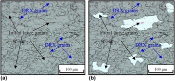
For the experimental material, it was found that the conventional method to calculate the DRX volume fraction based on true stress–strain curves is not suitable by the authors' previous works. Reference Chen, Lin, Li and Zhou34 So, the DRX volume fractions of deformed specimens were evaluated based on optical micrographs. Figure 4(a) shows the typical optical micrograph including fine DRX grains and initial large grains. Generally, the DRX volume fraction can be defined by:
 $${X_{{\rm{drx}}}} = {{{A_{{\rm{drx}}}}} \over {{A_t}}} = 1 - {{{A_{{\rm{initial}}}}} \over {{A_t}}}$$
in which A drx is the area of DRX grains. A t is the total area of optical micrograph, which is the sum of A drx and A initial. A initial is the area of initial grains which are not replaced by DRX grains. However, because the values of A drx and A initial are hard to directly measure via optical micrograph, the following equation is used to evaluate X drx Reference Chen, Lin, Li and Zhou34 :
 $${X_{{\rm{drx}}}} = 1 - {{{N_{{\rm{initial}}}}} \over {{N_{{\rm{total}}}}}}$$
in which N initial is the number of pixel of initial grains which are not replaced by DRX grains, and N total is the total number of pixel of optical micrograph. As shown in Fig. 4(b), the area of initial grains, which are not replaced by DRX grains (the white area), is chosen. The values of N initial and N total can be directly obtained by the Photoshop software. Therefore, for a given optical micrograph, the value of X drx can be evaluated by Eq. (17). Three different optical micrographs in the central area were applied to obtain X drx in the central part of deformed specimens (X drx,c).
Sketch maps for evaluating X drx using the photoshop software: (a) the initial optical micrograph; (b) the optical micrograph which is dealt with in the Photoshop software.

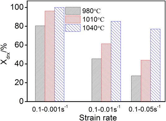
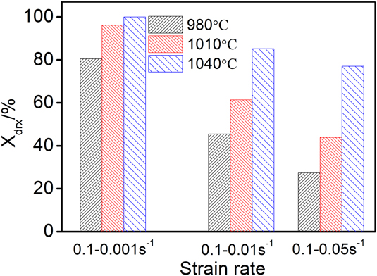
Based on the above-mentioned method, the values of X drx in the central part of deformed specimens (X drx,c) under tested conditions were obtained, as shown in Fig. 5. As shown in Fig. 5, the histories of strain rate significantly affect the DRX behavior of experimental material. The DRX volume fraction of deformed specimens increases with the decrease of strain rate in stage II. The law is similar to that under constant strain rate conditions. Reference Chen, Lin, Li and Zhou34 It mainly attributes that the critical dislocation density for the nucleation of DRX grains decreases with the decrease of strain rate, and the time for the growth of small DRX grains increases. In additional, the effects of deformation temperature on DRX behaviors under inconstant strain rate conditions are also similar to those under constant strain rate conditions. Reference Chen, Lin, Li and Zhou34 The DRX volume fraction of deformed specimens obviously increases with the increase of deformation temperature. It attributes to the increased mobility of grain boundaries with the increased deformation temperature.
DRX volume fractions in the central part of deformed specimens under tested conditions.
C. Evaluation of DRX volume fractions based on the improved DRX kinetics model
In this section, the DRX volume fractions in the central part of deformed specimens (X drx,c) are evaluated by the improved DRX kinetics model. To consider the friction-induced inhomogeneous deformation of specimens, finite element simulations have been done to obtain the strains and strain rates in the center of deformed specimens.
1. Finite element model to obtain the effective strain and strain rate
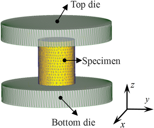
The established finite element (FE) model by DEFORM-3D software is shown in Fig. 6. The tetrahedral element was used in meshed specimen, and the number of elements is 20,000. During the simulation, a new FEM mesh on the specimen will be automatically generated whenever necessary, for example, the old mesh becomes unusable (negative Jacobian). The tabular data format is used to define the flow stress of experimental material, which is obtained from hot compressive tests. Reference Chen, Lin, Li and Zhou34 The boundary conditions of FE models are the same as those of hot compressive tests.
Finite element model for the simulation of hot compressive process.
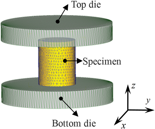
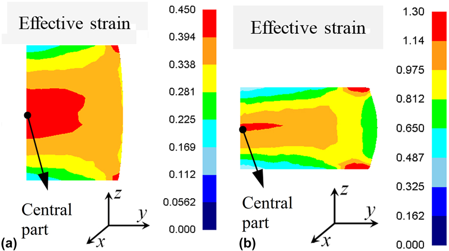
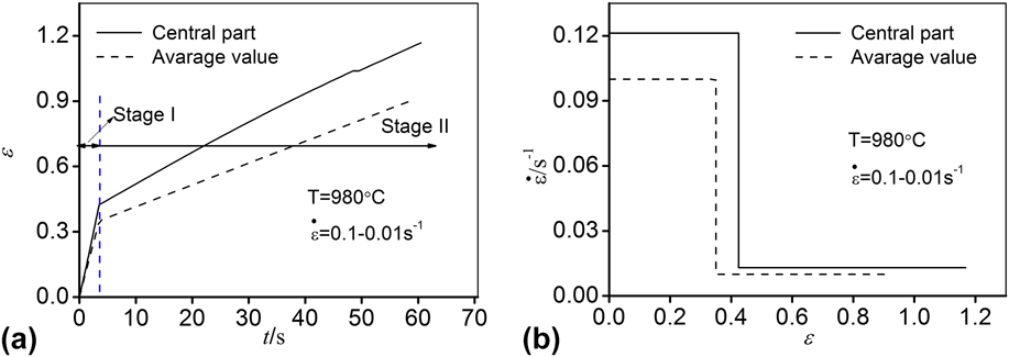
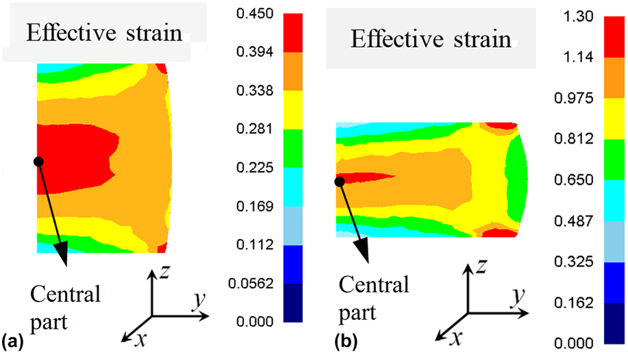
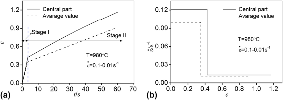
Figure 7 shows the typical distributions of effective strain in the compressive axis section of deformed specimens. As shown in Fig. 7, it can be found that the effective strain in the central part is obviously larger than the average value. Figure 8(a) illustrates that the relationship between the effective strain and time in the central part of typical deformed specimen (the deformation temperature is 980 °C and the strain rate is “0.1–0.01 s−1”). It can be found that the effective strain in the central part nearly linearly increases with time in stages I or II. Thus, the effective strain rates in stages I or II can be considered to be constant, as shown in Fig. 8(b). The values of effective strain and effective strain rate in the central part of deformed specimens obtained from FE simulation are shown in Table I.
Typical distributions of effective strain in the compressive axis section of deformed specimens at: (a) the end of stage I; (b) the end of stage II (half of the specimen).
Effective strains and effective strain rate in the central part of typical deformed specimen obtained by FE simulation: (a) relationship between the effective strain and time; (b) relationship between the effective strain rate and effective strain.
The values of εI,c, εII,c,
 ${\dot \varepsilon _{{\rm{I,c}}}}$
, and
 ${\dot \varepsilon _{{\rm{II,c}}}}$
obtained by FE simulations (εI,c and εII,c are the effective strains in the central part of deformed specimens at the end of stages I and II, respectively;
 ${\dot \varepsilon _{{\rm{I,c}}}}$
and
 ${\dot \varepsilon _{{\rm{II,c}}}}$
are the effective strain rates in the central part of deformed specimens in stages I and II, respectively).

2. Evaluation of DRX volume fractions in the central part of deformed specimens
The classic DRX kinetics models for the experimental material (a typical solution-treated Ni-based superalloy) were reported in authors' previous work. Reference Chen, Lin, Li and Zhou34
 $$\left\{ \matrix{ {X_{{\rm{drx}}}} = 1 - \exp \left[ { - 0.693{{\left( {{{\varepsilon - {\varepsilon _{\rm{c}}}} \over {{\varepsilon _{0.5}} - {\varepsilon _{\rm{c}}}}}} \right)}^{1.8}}} \right] \hfill \cr \hfill \cr {\varepsilon _{0.5}} = 6.43937 \times {10^{ - 6}}\,{{\dot \varepsilon }^{0.14281982}}\,\exp \left( {16038.638/T} \right) \hfill \cr {\varepsilon _{\rm{c}}} = 0.2315{\varepsilon _{0.5}} \hfill \cr} \right.$$
in which X
drx is the DRX volume fraction, ε is the strain, εc is the critical strain for the onset of DRX, ε0.5 is the strain for 50% DRX, T is the deformation temperature (unit: K), and
 $\dot \varepsilon$
is the strain rate (unit: s−1).
Substituting the material constants of Eq. (18) into Eq. (14), the improved DRX kinetics model for predicting DRX behavior under inconstant deformation temperature and strain rate conditions can be obtained as:
 $$\left\{ \matrix{ {\nu _{{\rm{drx}}}}\left( {T,\dot \varepsilon ,{X_{{\rm{drx}}}}} \right) = {{1.2474} \over {{\varepsilon _{0.5}} - {\varepsilon _{\rm{c}}}}}\left( {1 - {X_{{\rm{drx}}}}} \right){\left[ { - {1 \over {0.693}}\ln \left( {1 - {X_{{\rm{drx}}}}} \right)} \right]^{{4 \over 9}}} \hfill \cr \hfill \cr {\varepsilon _{\rm{c}}} = 1.49 \times {10^{ - 6}}\,{{\dot \varepsilon }^{0.14281982}}\,\exp \left( {16038.638/T} \right) \hfill \cr {\varepsilon _{0.5}} = 6.43937 \times {10^{ - 6}}\,{{\dot \varepsilon }^{0.14281982}}\,\exp \left( {16038.638/T} \right) \hfill \cr} \right.\quad {\rm{when}}\;{X_{{\rm{drx}}}} > 0$$
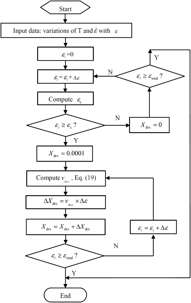
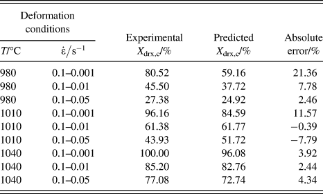
In order to evaluate the DRX volume fractions, a computer program based on the improved DRX kinetics model is developed. The flow chart is shown in Fig. 9. In Fig. 9, εtotal is the total effective strain, which is equal to εII,c for the central part of deformed specimens. Δε is the strain increment which should be enough small. In this paper, it is enough that Δε is 0.001 to accurately predict DRX volume fractions. Based on the data shown in Table I, the DRX volume fractions in the central part of deformed specimens under tested conditions are obtained, as listed in Table II.
Flow chart to evaluate the DRX volume fractions based on the improved DRX kinetics model.

Experimental and predicted X drx,c.
D. Comparisons between the experimental and predicted DRX volume fractions
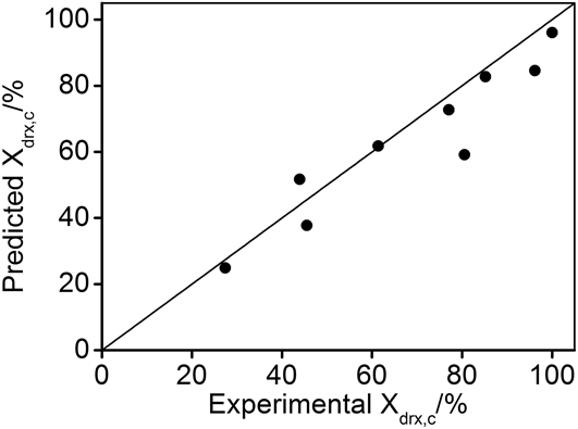
The comparisons between the experimental and predicted X drx,c are done, as shown in Fig. 10. It shows that the predicted X drx,c well agree with the experimental ones. The absolute errors between the experimental and predicted X drx,c are evaluated, as listed in Table II. The absolute errors are smaller than 8% for most cases. It indicates that the improved DRX kinetics model can well predict the DRX behavior of the solution-treated Ni-based superalloy under inconstant deformation temperature and strain rate conditions.
Comparisons between the experimental and predicted X drx,c.

IV. CONCLUSIONS
In practical industrial production, the deformation temperature and strain rate of forgings are often time-varying. However, the classical DRX kinetics models can only describe the DRX behavior under constant deformation temperature and strain rate conditions. Therefore, an improved DRX kinetics model, which can describe the DRX behavior under inconstant deformation conditions, is proposed. To verify the improved DRX kinetics model, the hot compressive tests with abruptly-changed strain rate were done on a solution-treated Ni-based superalloy. The comparisons between the experimental and predicted DRX volume fractions indicate that the improved DRX kinetics model is suitable for describing the DRX behavior of metals or alloys under inconstant deformation conditions.
ACKNOWLEDGMENTS
This work was supported by National Natural Science Foundation of China (Nos. 51305466, 51375502), National Key Basic Research Program (Grant No. 2013CB035801), State key laboratory of High Performance Complex Manufacturing (No. zzyjkt2014-01), the Project of Innovation-driven Plan in Central South University (Grant No. 2016CX008), the Natural Science Foundation for Distinguished Young Scholars of Hunan Province (Grant No. 2016JJ1017), and Program of Chang Jiang Scholars of Ministry of Education (Grant No. Q2015140), China.