


1. Introduction
By mimicking the flexible movements of the human lower limbs, bipedal robots can navigate complex terrains such as stairs and slopes, thus overcoming the environmental limitations of traditional wheeled robots. Their upright posture better meets human–robot interaction needs, enabling natural collaboration in many fields such as service and healthcare. Currently, research on the walking dynamics of bipedal robots involves multiple fields, with many aspects still warranting in-depth study. These areas encompass gait stability and transition [Reference Sun, Zhou, Xu and Wang1, Reference Shin and Ikemoto2], the application of intelligent algorithms [Reference Mahapatro, Dhal, Parhi, Muni, Sahu and Patra3], optimization of energy efficiency [Reference Chen, An, Wang, Miao, Song and Shangguan4, Reference Hanazawa, Uchino and Sagara5], the design of motion control systems [Reference Zhang, Liu and Tan6], bio-inspired leg design [Reference Xie, Li, Lu, Li, Hu and Gao7], among others.
Gait stability analysis is critical for bipedal robot control, as it directly governs the robot’s ability to maintain balance in complex and unpredictable environments. In-depth research on gait stability helps scientists develop more robust control algorithms and optimized robotic structures, thereby enhancing reliability and adaptability in practical application. Stable gait not only ensures task execution safety but also reduces energy consumption, extends operational duration, and lays the foundation for broader application scenarios. Key methods for assessing gait stability include the energy stability criterion [Reference Xie, Gao, Zhu, Yan, Kong, Xie, Gu and Zhang8], Lyapunov stability analysis [Reference Kolathayaa and Amesa9], balance recoverability [Reference Mihalec, Trkov and Yi10], Floquet theory [Reference Zhou, Hui, Chen and Jiang11], among others.
The period-
 $1$
gait, in which the motion trajectory of the robot is exactly the same for each step, is a highly symmetric and stable limit cycle. Due to its constant step length, period, and energy consumption, the period-
 $1$
gait is the most common, stable, and easiest to achieve [Reference Li, Tang and Yang12–Reference Hobon, De-León-Gómez, Abba, Aoustin and Chevallereau14]. Appropriate initial conditions are critical for bipedal robot stable walking, especially for passive limit cycles with small attraction basins, and a related work proposed a BVP-IVP-continuation method to determine such conditions for compass-gait robots’ period-1 gaits, verifying their key impact on periodic gait convergence via parametric analysis [Reference Safartoobi, Dardel, Ghasemi and Daniali15]. The period-
 $N$
gait, which requires
 $N$
steps
 $(N\gt 1)$
to complete a full gait cycle [Reference Gritli, Belghith and Khraief16], exhibits predictable fluctuations and usually represents a transitional phase where the gait becomes unstable and evolves into more complex behaviors.
The chaotic gait, characterized by non-repeating motion and high sensitivity to initial conditions, demonstrates random and unpredictable step lengths and periods, making the robot prone to falling. Due to its unpredictable motion patterns and the potential for causing the robot to fall, the chaotic gait is desired to be controlled into a periodic gait. Currently, the classical Ott–Grebogi–Yorke (OGY) method [Reference Iqbal, Zang, Zhu and Zhao17–Reference Khan and Mandava19] and various improved OGY methods [Reference Gritli and Belghith20–Reference Taghvaei and Vatankhah22] whose core concept involves controlling chaotic gait to an unstable periodic gait embedded in attractors through minute parameter perturbations are widely employed to control chaotic gaits, with most subjects of study being passive dynamic bipedal robots.
Chaos often arises through a series of bifurcations (such as period-doubling bifurcations). Bifurcation control is another effective method for regulating chaotic gaits. It involves identifying and adjusting key parameters to delay, alter, or eliminate bifurcations, thereby transforming a chaotic gait into a stable periodic gait. In Ref. [Reference Zhou, Hui, Chen and Jiang11], the chaotic gait of a semi-passive compass-like robot is controlled into stable periodic gait by adjusting the angle between the two legs at impact. The occurrence of the flip bifurcation is delayed, and the gait is controlled to a stable period-
 $1$
gait by adjusting the leg extension ratio [Reference Zhou, Hui, Chen and Jiang11, Reference Jiang, Jiang, Liu and Jiang23].
In addition to OGY method and bifurcation control method, scholars have been continuously exploring effective approaches for controlling chaotic gaits, such as trajectory tracking approach [Reference Added, Gritli, Belghith and Zhang24], delayed feedback control [Reference Harata, Asano, Taji and Uno25], kinetic energy shaping [Reference Tereshko26], neural network-based adaptive predictive feedback control [Reference Zhang, Zhou, Wang, Liu and Wu27], among others.
There are also research conclusions regarding the control of multi-period (period-
 $N$
) gaits to period-
 $1$
gait. For underactuated bipedal robots, a hybrid control strategy (such as event triggered phase switching), which depends on the coordination of foot contact force and centroid motion, is implemented to achieve transition from multi-period gaits to period-1 gait [Reference Yuan, Ge and Gan28]. In addition, the bifurcation control method is used to control multi-period gaits to stable period-
 $1$
gaits [Reference Jiang, Jiang, Liu and Jiang23].
Research on gait control, including the control of chaotic gaits, has predominantly focused on passive walking gaits downhill on slopes without external driving forces. However, when bipedal robots walk on flat or more complex terrains, driving forces become necessary, making gait control more complex. Driving forces can be continuous or impulse-driven. While the theoretical advantages of impulsive actuation, such as its potential for reducing energy consumption, have been established, its practical implementation presents unique engineering challenges. In practice, impulsive actuation can be realized through various mechanisms, such as spring-loaded mechanisms [Reference Yoshimi, Mori and Kobayashi29, Reference Laschowski and McPhee30] that store and release energy intermittently, pneumatic/hydraulic pulse systems [Reference Park, Kim, Gong, Yang, Hwang, Jung, Moon, Koo, Rodrigue and Choi31–Reference Jiang and Zhang33] that generate short-duration high-force impulses, series elastic actuators with impact elements [Reference Cappello, Xiloyannis, Dinh, Pirrera, Mattioni and Masia34, Reference Le and Nguyen35], and electromagnetic impulse generators [Reference Duduta, Berlinger, Nagpal, Clarke, Wood and Temel36, Reference Yang, Wang, Zhang, Yang and Leng37].
In the field of bipedal robotic gait control, while notable progress has been made, significant gaps remain in the study of gait control of bipedal robots with impulsive actuation, necessitating further in-depth research:
(1) Control methods for transforming from chaotic gaits to period-
 $1$
gaits and their comparison
While the OGY method achieves chaos control with minimal perturbation, its suitability for rapidly controlling chaotic gaits in robots requires further investigation. Bifurcation control in literature is implemented by adjusting the angle between the two legs at the impact [Reference Zhou, Hui, Chen and Jiang11] and leg extension ratio [Reference Jiang, Jiang, Liu and Jiang23] – whether this is practically feasible or easily controllable remains uncertain. This study explores a more straightforward approach: applying constant thrust increments to control chaotic gaits.
(2) Converting multi-period gaits into period-
 $1$
gaits
Period-
 $1$
gaits offer the highest level of predictability, stability, and energy efficiency. Although multi-period gaits are predictable compared to chaotic gaits, stabilizing them into period-
 $1$
gaits significantly enhances the robot’s disturbance rejection capability. This ensures recovery to a unique stable motion pattern despite parametric variations or external disruptions. However, research conclusions in this area remain limited.
(3) Controlling the parameter range for stabilizing period-
 $1$
gaits
Studying the stable parameter range of period-
 $1$
gaits is critically significant as it provides a theoretical foundation and design boundaries for practical, reliable, and high-performance bipedal robots. Quantifying the “stability domain” of the period-
 $1$
allows engineers to avoid unstable regions that may lead to bifurcation or chaos, thereby ensuring fundamental operational reliability. A broad stable parameter range implies strong robustness, enabling the robot to maintain stable periodic motion under internal parameter variations and external disturbances, thereby significantly improving its adaptability to varying environments. To our knowledge, systematic studies in this direction are still lacking.
Driven collectively by the aforementioned factors, this study aims to develop an impulse-based control scheme to stabilize bipedal locomotion into a period-
 $1$
gait with a maximized stability region. Paper [Reference Long, Hui and Jiang38] studied the existence of periodic gaits and their bifurcations in a bipedal robot with impulsive actuation. Bipedal walking dynamics are extremely complex. Building upon the work in Ref. [Reference Long, Hui and Jiang38], this study further investigates another critical aspect: walking gait control.
The novelty of this study relative to existing literature is threefold: (1) focusing on impulse-driven bipedal robots for level-ground walking (a less explored object) instead of passive dynamic walkers; (2) proposing a bifurcation control method based on pulse thrust parameter optimization (feasible for engineering) instead of traditional mechanical structural parameter adjustment; and (3) deriving the quantitative parameter interval for expanding period-1 gait stability domain and realizing stable conversion of multiple multi-period gaits to period-1 gaits. The study is organized as follows. A brief introduction to the bipedal robot walking model with impulsive actuation is given in the next section, along with the selection of gaits under certain constraints as the controlled gaits. Chaotic gait control methods are investigated in Section 3, while the control of multi-period gaits is discussed in Section 4. The controlling of the parameter range for stabilizing period-
 $1$
gaits in Section 5 and conclusion is given in Section 6.
2. Walking model and controlled gaits
2.1. Bipedal robot walking model with impulsive actuation
Unlike constant torques drive (see Figure 1(a)), the impulsive actuation (see Figure 1(b)) applies a pulse torque
 $u$
to the hip joint and a pulse thrust
 $ P=a(\dot \theta _{s}^-)^2+b\dot \theta _{s}^-+c$
to the heel of the stance leg at the heel strike moment to provide power for the bipedal robot to walk on level ground.
For the 2-DOF bipedal robot with impulsive actuation, the robot has two rigid straight legs of length l and equal mass m, with the mass M of the upper body and trunk concentrated at the hip joint,
 $\theta _{s}$
and
 $\theta _{ns}$
denote the angles of stance leg and the swing leg with respect to the ground normal, respectively, and
 $\alpha$
is the angle between the two legs.
The gait cycle of bipedal robots comprises a swing phase, an impact phase, and an alternation between the support leg and swing leg. The swing motion of each step continues until the occurrence of impact condition, which is given as follows:
 \begin{equation} \Omega = \left \{ {({\theta _s},\ \dot \theta _{s},\ {\theta _{ns}},\ \dot \theta _{ns} )\left | \theta _s(t) = -\frac {\gamma }{2}, \theta _{ns}(t) = \frac {\gamma }{2} \right .} \right \}\!. \end{equation}
Schematic representation of a bipedal robot walking model: (a) constant torques
 $u_1$
and
 $u_2$
and (b) pulse torque
 $u$
and pulse thrust
 $P$
.

Figure 1 Long description
The image shows a schematic representation of a bipedal robot walking model. In part (a), the model is depicted with constant torques labeled as u1 and u2. The diagram includes angles alpha and theta2, a mass M at the top, and a mass m at the bottom, connected by a leg of length l. The angles and torques illustrate the forces and positions during walking. In part (b), the model is shown with a pulse torque labeled as u and a pulse thrust labeled as P. The angles alpha and gamma are equal, indicating a specific phase of the walking cycle. The diagram also shows the heel strike position, illustrating the transition between steps. The overall structure highlights the mechanical dynamics and control mechanisms of the bipedal robot's walking pattern.
Let
 \begin{equation*} x=(x_{1}(t),\ x_{2}(t),\ x_{3}(t),\ x_{4}(t))^T=(\theta _{s}(t),\ \dot \theta _{s}(t),\ \theta _{ns}(t),\ \dot \theta _{ns}(t))^T. \end{equation*}
The walking model of a bipedal robot with impulsive actuation is obtained as follows:
 \begin{equation} \begin{array}{ll} \dot x=f(x), \ \ \ x\notin \Omega ,\\ x^+=H (x^-,\ P,\ u), \ x\in \Omega , \end{array} \end{equation}
where
 \begin{align*} \left . \begin{array}{ll} f(x)=\left (x_{2}(t),\ x_{1}(t),\ x_{4}(t),\ x_{1}(t)-x_{3}(t)\right )^T,\\[4pt] \Omega = \left \{ {(x_1,\ x_2,\ x_3,\ x_4 )\left | x_1(t) = -\dfrac {\gamma }{2}, x_3(t)= \dfrac {\gamma }{2}\right .} \right \}\!,\\[8pt] H (x^-,\ P,\ u)= \big(x_{3}^-,\ x_{1}^-\cos \gamma +\dfrac {P}{lM} \sin \gamma , \ x_{1}^-,\ x_{4}^-\cos \gamma + \dfrac {P}{lM} \sin \gamma \cos \gamma +u \big)^T. \end{array} \right . \end{align*}
Let
 $\Omega$
be the Poincaré section, where
 $\Omega$
is shown in (1). Suppose a trajectory of system (2) reaches the point
 $A_{k}(\!-\frac {\gamma }{2},\ x_{2k},\ \frac {\gamma }{2},\ x_{4k})$
on
 $\Omega$
. The trajectory jumps from the point
 $A_{k}$
to the point
 $\bar {A}_{k}(\frac {\gamma }{2},\ \bar {x}_{2k},\ -\frac {\gamma }{2},\ \ \bar {x}_{4k})$
, which is on
 $\Gamma = \left \{ {(x_1,\ x_2,\ x_3,\ x_4 )\left | x_1(t) = \frac {\gamma }{2}, x_3(t)= -\frac {\gamma }{2}\right .} \right \}\!.$
This trajectory originating from the initial point
 $\bar {A}_{k}$
reaches the point
 $A_{k+1}(\!-\frac {\gamma }{2},\ \ x_{2(k+1)},\ \frac {\gamma }{2},\ \ x_{4(k+1)})$
at
 $t=\tau$
, where
 $A_{k+1} \in \Omega$
and
 $\tau$
is called a step period.
These two points
 $A_k$
and
 $A_{k+1}$
are used to construct the following two-dimensional map:
 \begin{align*} \left \{ \begin{array}{ll} x_{2(k+1)}=cos\gamma {x}_{2k}+\dfrac { sin\gamma (a x^2_{2k}+b x_{2k}+c )}{lM},\\[9pt] x_{4(k+1)}=\dfrac {0.75\gamma (cos\tau +1)}{sin\tau }+0.5\left ( cos\gamma {x}_{2k}+\dfrac { sin\gamma (a x^2_{2k}+b x_{2k}+c )}{lM} \right )\!, \end{array} \right . \end{align*}
where
 $x_{4(k+1)}$
is determined by
 $x_{2k}$
. The first sub-map of the above map, which is rewritten as the following Poincaré map by assuming
 $x_{2k}=y_{k}$
and setting
 $A=\frac {sin\gamma }{lM}$
:
 \begin{equation} y_{k+1}=Aa y^2_{k}+(Ab+\cos \gamma )y_k+Ac=g(y_{k}, b), \end{equation}
where
 $b$
is treated as a parameter.
For a given fixed point
 $y_{0}$
of the Poincaré map (3), the point
 $A^{*}(\!-\frac {\gamma }{2},\ y_{0},\ \frac {\gamma }{2},\ \frac {0.75\gamma (\cos \tau +1)}{\sin \tau }+0.5y_{0})$
corresponds to one period-
 $1$
gait of (2), where the pulse thrust
 $P$
, the pulse torque
 $u$
, and the step period
 $\tau$
are given as follows:
 \begin{equation} P=ay_{0}^2+by_{0}+c,\ u=\frac {0.75\gamma (1+\cos \tau )}{\sin \tau }+(0.5-\cos \gamma )y_{0},\ \tau =\ln \frac {2y_{0}-\gamma }{2y_{0}+\gamma }. \end{equation}
For more details on the bipedal robot model (2) with impulsive actuation and the Poincar
 $\acute {\textrm { e}}$
map (3), refer to Ref. [Reference Long, Hui and Jiang38] and related references cited therein. In the bipedal robot model (2), angular momentum conservation is adopted to model the impact phase, primarily because it is highly consistent with the Lagrangian dynamics used for the swing phase and naturally accommodates the leg role exchange without requiring pointwise impact force analysis. Additionally, the nonlinear impulse thrust introduced in this paper, which is applied at the ankle of the stance leg and directed toward the hip, can be conveniently integrated into the impact mapping via angular momentum conservation, whereas Newton’s impact law would necessitate extra modeling of the coupling between thrust and contact forces. It is acknowledged that Newton’s impact method was employed for systematic modeling of multi-link bipedal robots, which offers good scalability for multi-rigid-body collisions [Reference Fazel, Shafei and Nekoo39]. In future work, a comparison of both approaches is planned to further validate the applicability and robustness of the proposed modeling strategy.
The construction of Poincaré maps plays a crucial role in studying the walking dynamics of bipedal robots. For instance, an explicit-form Poincaré map is developed to discuss passive dynamic walking [Reference Znegui, Gritli and Belghith40], a controlled Poincaré map is designed to analyze the stabilization of the passive walking dynamics, thereby deriving an effective state-feedback control law in Ref. [Reference Znegui, Gritli and Belghith41]. A key distinction to note is that the control term in the controlled Poincaré map in Ref. [Reference Znegui, Gritli and Belghith41] is a continuous torque
 $u$
applied during the swing phase, while in this study, no continuous torque is considered. Instead, the control term in the developed Poincaré map (3) is related to the pulse thrust
 $P$
, which acts during the instantaneous collision-switching phase.
The walking model with impulsive actuation (2) can be practically implemented through spring-based impulsive mechanism. Compression springs or torsional springs can be used to store energy during the swing phase and release it as an impulsive thrust at heel strike. This approach enables energy recovery from the robot’s own dynamics and has been successfully implemented in passive dynamic walkers. By adjusting the spring stiffness and pre-compression, the theoretical pulse thrust parameters
 $(a,\ b,\ c)$
are mapped to actual control variables, thereby regulating the pulse thrust
 $ P=a(\dot \theta _{s}^-)^2+b\dot \theta _{s}^-+c$
. The pulse thrust must be precisely synchronized with heel strike, requiring high-bandwidth force/torque sensors at the foot.
It is worth noting that
 $y_0\lt 0$
due to the fact that the angular velocity of the stance leg
 $\dot \theta _{s}\lt 0$
in actual walking. Therefore, one negative fixed point of the Poincaré map (3) corresponds to one period-
 $1$
gait of (2) and vice versa.
2.2. Controlled gaits
For the pulse thrust
 $ P=a(\dot \theta _{s}^-)^2+b\dot \theta _{s}^-+c$
, first assume that the parameters
 $a\gt 0$
and
 $c\geq 0$
. Map (3) has two negative fixed points:
 \begin{equation} y_{ 0 1} = \frac {-(Ab+\cos \gamma -1)- \sqrt {\Delta _1 }}{2Aa},\ y_{ 0 2} =\frac {-(Ab+\cos \gamma -1)+ \sqrt {\Delta _1 }}{2Aa}, \end{equation}
for
 $b\gt b_1$
, where
 $ \Delta _1=(Ab+\cos \gamma -1)^2-4A^2ac$
and
 \begin{equation} b_1=\frac {2A\sqrt {ac}+1-\cos \gamma }{A}. \end{equation}
The fixed point
 $ y_{ 0 2}$
, which eigenvalue
 $ \lambda _{03}=1+\sqrt {\Delta _1 }\gt 1,$
corresponds to an unstable period-
 $1$
gait of (2).
The eigenvalue of the fixed point
 $ y_{ 0 1}$
is
 \begin{equation*} \lambda _{01}=g'(y_{k}, b)|_{y_{k}=y_{ 0 1}}=2Aa y_{0}+Ab+\cos \gamma =1-\sqrt {\Delta _1 }. \end{equation*}
It is easy to calculate that
 $\lambda _{01}=1$
at
 $b=b_1$
while
 $\lambda _{01}=-1$
at
 \begin{equation} b=b_2=\frac {2\sqrt {1+A^2ac}+1-\cos \gamma }{A}. \end{equation}
Hence, a fold bifurcation occurs at
 $b=b_1$
and a flip bifurcation occurs at
 $b=b_2$
. For
 $b\in (b_1,\ b_2)$
,
 $|\lambda _{01} | \lt 1$
and the fixed point
 $ y_{ 01}$
corresponds to a stable period-
 $1$
gait of (2).
In Model (2), the parameters for the robot are set as
 $l=1m$
,
 $\gamma =0.4 rad$
, and
 $M=10kg$
. For the pulse thrust
 $ P=a(\dot \theta _{s}^-)^2+b\dot \theta _{s}^-+c$
, set
 $a=12$
and
 $c=8$
. It follows from (6) and (7) that
 $b_1=21.6230$
and
 $b_2=56.9972$
. Figure 2 shows that as parameter
 $b$
varies (
 $b\gt b_1=21.6230$
), flip bifurcations occur, consequently giving rise to multi-periodic gaits (
 $P-n,\ n=2,\,4,\ \cdots$
) and chaotic gaits.
The bifurcation diagram of periodic gaits with respect to
 $b$
for system (2) with
 $a=12$
and
 $c=8$
.

Figure 2 Long description
A line graph showing the bifurcation diagram of periodic gaits with respect to b for a system with a equals 12 and c equals 8. The x axis represents the variable b ranging from negative 70 to 80. The y axis represents the variable x 2 k ranging from negative 10 to 6. The graph includes a red dashed line indicating unstable P minus 1 gait, a blue solid line indicating stable P minus 1 gait, and red arrows pointing to fold bifurcation and flip bifurcation. Key points on the x axis are marked at b equals negative 17.5688, b 1 equals 21.6230, and b 2 equals 56.9972. The graph shows complex behavior with regions of stability and instability. All values are approximated.
The stable period-
 $1$
gait is the most ideal walking mode for bipedal robots. There exist multi-period gaits and chaotic gaits for
 $b\gt b_2$
in the case of
 $a\gt 0$
and
 $c\geq 0$
, which need to be controlled to period-
 $1$
gait. There is no fixed point in (3) for
 $b\in (\!-17.5688,\ b_1)$
, and there are only positive fixed points in (3) for
 $b\lt -17.5688$
; hence, there is no periodic gait for
 $b\lt b_1$
in the case of
 $a\gt 0$
and
 $c\geq 0$
, which leaves room for us to explore the existence of period-
 $1$
gait. Thus, the gaits of walking model (2) in the case of
 $a\gt 0$
and
 $c\geq 0$
are designated as the target gaits for control to discuss walking gait control.
To study the gait control of bipedal robots, it is also necessary to consider the initial conditions for gait simulation. All numerical simulations in this study employ initial conditions selected according to the following systematic methodology.
Phase space analysis: Initial states are chosen based on the system’s phase portrait and Poincaré map analysis. For chaotic gait simulations, points are selected from within the chaotic attractor.
Physical consistency check: Initial states are chosen based on practical joint limits
 $|\theta _{s}|,\ |\theta _{ns}|\lt \frac {\pi }{3}$
and angular velocities limits
 $\pm 10 rad/s$
.
Bifurcation-informed selection: For period-
 $1$
gait analysis, initial conditions are taken as fixed point of the Poincaré map (3) and its nearby points. For period-
 $2,4,\cdots$
gaits analysis, points are selected from corresponding periodic orbits and their neighborhoods.
Robustness verification: Multiple initial conditions from different regions of the state space are tested to ensure control strategies are not overly sensitive to specific starting points.
Different from the BVP-based initial condition determination method for passive compass-gait bipedal robots [Reference Safartoobi, Dardel, Ghasemi and Daniali15], the above strategy is specifically developed for the impulse-driven bipedal robot model in this study, which fully considers the dynamic characteristics of impulsive actuation at heel strike and the bifurcation behavior of the system. It not only ensures the physical rationality of initial states but also guarantees the relevance of initial conditions to the controlled gait types (chaotic, multi-period, and period-1), which is essential for the validity of the subsequent gait control simulation results.
3. Chaotic gait control
3.1. OGY control
Assume that system (2) is chaotic at
 $b=b_0$
(see Figure 3(a)). The period-
 $1$
gait, which corresponds to the fixed point
 $y_{01}$
for
 $b=b_0$
in (5), is unstable and embedded within the attractor. Now calculate the small disturbance about parameter
 $b$
.
At
 $(b_0,\ y_{01})$
, it follows from (3) that
 \begin{equation*} \begin{array}{cc} & \dfrac {\partial g} {\partial y_k}(b_0,\ y_{01})= 2Aa y_{01}+Ab_0+\cos \gamma ,\\ & \dfrac {\partial g} {\partial b}(b_0,\ y_{01}) = Ay_{01}. \end{array} \end{equation*}
By linearizing the Poincaré map (3) around
 $(b_0,\ y_{01})$
, we derive the perturbation parameter as:
 \begin{equation} \bar {b}=-\dfrac {\dfrac {\partial g} {\partial y_k}}{\dfrac {\partial g} {\partial b}}(b_0,\ y_{01})=\frac {2Aa y_{01}+Ab_0+\cos \gamma }{Ay_{01}}=\frac {\sqrt {\triangle _1}-1}{Ay_{01}}. \end{equation}
For system (2) with
 $a=12$
and
 $c=8$
, (a) the bifurcation diagram of periodic gaits with respect to
 $b$
and (b) the maximum Lyapunov exponent with respect to
 $b$
.

Figure 3 Long description
The image contains two graphs. The first graph, labeled (a), is a bifurcation diagram showing the relationship between the variable x2k and the parameter b. The diagram features a blue line representing the system's behavior and a red dashed line indicating a specific threshold or boundary. The second graph, labeled (b), displays the maximum Lyapunov exponent as a function of the parameter b. This graph also includes a blue line representing the Lyapunov exponent values and a red dashed line marking a critical threshold. Both graphs highlight a vertical dashed line at b = b0, indicating a significant point of interest. The bifurcation diagram illustrates the stability and transitions of periodic gaits, while the Lyapunov exponent graph shows the system's sensitivity to initial conditions and the presence of chaotic behavior. The graphs collectively demonstrate the dynamic behavior of the bipedal robot system under varying parameter conditions.
The controlled system is
 \begin{equation*} \left \{ \begin{array}{ll} \dot x=f(x), \ \ \ x\notin \Omega ,\\ x^+=H_{1}x^-+H_{2}\dfrac {\bar {P}}{lM}+H_{3}, \ x\in \Omega , \end{array} \right . \end{equation*}
where
 \begin{equation*} \bar {P}=a(x_2(t)^-)^2+(b+ \mu \bar {b}) x_2(t)^- +c, \end{equation*}
 \begin{equation} \mu =\left \{ \begin{array}{ll} 1, \ \ \ \textrm {if}\ x_1(t)= - \dfrac {\gamma }{2}\ \textrm {and}\ |x_2(t)-y_{01}|\lt \sigma ,\\ 0, \ \ \textrm {else}, \end{array} \right . \end{equation}
 $\mu$
is the switching function and
 $\sigma$
is the threshold value for state perturbation. Hence, the following result regarding chaotic gait control using the OGY control method is obtained.
Proposition 1.
Suppose that there is a chaotic gait in (
2
) under the controlling pulse thrust
 $P=a(x_2(t)^-)^2+b x_2(t)^- +c$
with
 $a\gt 0$
,
 $c\geq 0$
, and
 $b=b_0$
. This chaotic gait can be controlled to the period-
 $1$
gait by adding the pulse thrust
 $\bar {P}=a(x_2(t)^-)^2+(b+ \mu \bar {b}) x_2(t)^- +c$
, where
 $\bar {b}$
and
 $\mu$
are shown in (
8
) and (
9
), respectively.
For the parameters set
 $a=12$
,
 $c=8$
, and
 $b=b_0=73$
identified as chaotic in Figure 3(a), compute the maximum Lyapunov exponent to quantify the system’s sensitivity to initial conditions. The maximum Lyapunov exponent
 $\lambda _{max}$
is calculated using the following standard algorithm (see [Reference Yang and Wu42, Reference Gritli and Belghith43] and related references cited therein):
 \begin{equation*} \lambda _{max}=\lim _{t \to \infty } \frac {1}{t} \frac {|\delta X(t)|}{|\delta X(0)|}, \end{equation*}
where
 $\delta X(t)$
is the separation between initially close trajectories. Numerical computation yields the maximum Lyapunov exponent
 $\lambda _{max}=0.2735\gt 0$
for
 $b_0=73$
(see Figure 3(b)), confirming the chaotic gait.
In view of (5) and (8), one can calculate that
 \begin{equation*} y_{01}=-5.7995,\ \ \bar {b}= -7.3343. \end{equation*}
Hence, the controlling pulse thrust is
 \begin{equation} \bar {P}=12(x_2(t)^-)^2+(73- 7.3343 \mu ) x_2(t)^- +8, \end{equation}
where
 \begin{equation*} \mu =\left \{ \begin{array}{ll} 1, \ \ \ \textrm {if}\ x_1(t)= - \dfrac {\gamma }{2}\ \textrm {and}\ |x_2(t)+5.7995|\lt 0.9,\\ 0, \ \ \textrm {else}, \end{array} \right . \end{equation*}
Consider a chaotic gait starting from the point
 $(0.2000,\ -5.1495,\ -0.2000,\ 5.1417)$
, which is selected based on the requirements outlined in Section 2, including the chaotic attractor, joint limits, and angular velocity constraints.
Proposition1 provides a theoretical prediction for stabilizing the above chaotic gait through parameter perturbation of
 $\bar {b}$
. To validate this prediction, the controlling pulse thrust (10) with
 $\sigma =0.9$
is added to the bipedal robot at the
 $k$
-th step by using OGY control method (
 $k_{OC}$
). As shown in Figure 4(a), after implementing control at step
 $k_{OC}=16$
, the chaotic gait converges to the target period-1 orbit. The phase-plane trajectory in Figure 4(b) intuitively depicts the dynamic evolution of the system state from the chaotic attractor to the stable period-1 limit cycle in the state space, directly reflecting the suppression of chaotic motion by the OGY control method. The phase-plane plot of the stabilized period-1 gait (Figure 4(c)) further characterizes the bounded and periodic dynamic behavior of the controlled system, while the time series of the stance leg angular velocity (Figure 4(d)) verifies the steady-state performance of the controlled gait in the time domain.
For system (2) with
 $a=12$
,
 $c=8$
,
 $b=b_0=73$
, and the controlling pulse thrust (10) with
 $\sigma =0.9$
at
 $k_{OC}=16$
, (a) time series of
 $x_{2k}$
, (b) the chaotic gait is controlled to the target period-
 $1$
gait, (c) phase-plane plot of the stabilized period-1 gait in
 $x_1(x_3)$
-
 $x_2(x_4)$
space, and (d) time series of the stance leg angular velocity
 $x_2$
(
 $deg/s$
).

Figure 4 Long description
The image contains four graphs illustrating the control of chaotic gaits in a bipedal robot. The first graph (a) shows the time series of x2k, with a vertical axis labeled x2k in degrees per second and a horizontal axis labeled k. The second graph (b) presents a 3D plot comparing the chaotic gait and the target period-1 gait, with axes labeled x1, x2, and x3. The third graph (c) is a phase-plane plot of the stabilized period-1 gait in x1(x3) - x2(x4) space, with stance leg and swing leg trajectories marked in red and blue, respectively. The fourth graph (d) displays the time series of the stance leg angular velocity x2 in degrees per second over time t. The graphs collectively demonstrate the stabilization of chaotic gaits to a period-1 gait using controlling pulse thrust.
3.2. Bifurcation control
Suppose that there is a chaotic gait in (2) under the pulse thrust
 $P=a(x_2(t)^-)^2+b x_2(t)^- +c$
, where
 $b=b_0$
. Now suppress the occurrence of the first flip bifurcation and stabilize the chaotic gait to periodic gaits by adjusting the value of
 $c$
. Further suppose that the controlling pulse thrust is
 \begin{equation*} \bar {P}=a(x_2(t)^-)^2+b x_2(t)^- +C. \end{equation*}
It follows from (7) that the first flip bifurcation occurs at
 $b=\bar {b}_2=\frac {2\sqrt {1+A^2aC}+1-\cos \gamma }{A}$
under the controlling pulse thrust
 $\bar {P}$
. If
 $\bar {b}_2\gt b_0$
, the robot’s gait is no longer chaotic but is converted into a period-1 gait. In view of the fact that the period-
 $1$
gait after control is stable for
 $b\in (\bar {b}_1,\ \bar {b}_2)$
, the following condition needs to hold:
 \begin{equation*} \bar {b}_1\lt b_0\lt \bar {b}_2, \end{equation*}
where
 $\bar {b}_1=\frac {2A\sqrt {aC}+1-\cos \gamma }{A}$
. It follows that
 \begin{equation*} \frac {2A\sqrt {aC}+1-\cos \gamma }{A} \lt b_0\lt \frac {2\sqrt {1+A^2aC}+1-\cos \gamma }{A}, \end{equation*}
 \begin{equation*} c_1\lt C\lt c_2, \end{equation*}
where
 \begin{equation} c_1=\frac {(A b_0-1+ \cos \gamma )^2-4}{4A^2 a},\ c_2=\frac {(A b_0-1+ \cos \gamma )^2}{4A^2 a}. \end{equation}
Hence, the following result about chaotic gait control by using bifurcation control method is obtained.
Proposition 2.
Suppose that there is a chaotic gait in (
2
) under the pulse thrust
 $P=a(x_2(t)^-)^2+ b x_2(t)^- +c$
with
 $a\gt 0$
,
 $c\geq 0$
, and
 $b=b_0$
. This chaotic gait can be controlled to a period-
 $1$
gait by adding the pulse thrust
 $\bar {P}=a(x_2(t)^-)^2+b_0 x_2(t)^- +C$
, where
 $c_1\lt C\lt c_2$
,
 $c_1$
and
 $c_2$
are shown in (
11
).
As shown in the above, the robot’s gait is chaotic for
 $a=12$
,
 $c=8$
, and
 $b=b_0=73$
. In view of (11), one can calculate that
 \begin{equation*} c_1=49.9884,\ \ c_2=104.9407. \end{equation*}
In this case, Proposition2 determines the stable parameter range for successfully achieving bifurcation control as
 $49.9884\lt C \lt 104.9407$
. Numerical simulations are presented by setting
 $C=52$
.
The bifurcation diagrams of periodic gaits with respect to
 $b$
for system (2) with pulse thrust
 $P=a(x_2(t)^-)^2+b x_2(t)^- +c\ (a=12,\ c=8)$
and controlling pulse thrust
 $\bar {P}=a(x_2(t)^-)^2+b x_2(t)^- +C\ (a=12,\ C=52)$
.

Figure 5 Long description
The line graph shows the bifurcation diagrams of periodic gaits with respect to b for a system with pulse thrust P and controlling pulse thrust P bar. The x-axis represents the parameter b, ranging from 20 to 90. The y-axis represents x subscript 2k, ranging from -10 to 2. The graph includes two main data sets: one in blue for P equals a times x subscript 2t minus squared plus b times x subscript 2t minus plus c with a equals 12 and c equals 8, and another in red for P bar equals a times x subscript 2t minus squared plus b times x subscript 2t minus plus C with a equals 12 and C equals 52. The blue line shows a bifurcation at b equals 35.3742, while the red line shows a bifurcation at b equals 12.6837. The graph illustrates the transition from chaotic and multi-period gaits to period-1 gaits through bifurcation control and the expansion of stable parameter regions. All values are approximated.
For system (2) with
 $a=12$
,
 $c=8$
,
 $b=b_0=73$
, and the controlling pulse thrust
 $\bar {P}=12(x_2(t)^-)^2+73 x_2(t)^- +52$
at
 $k_{BC}=16$
, (a) time series of
 $x_{2k}$
, (b) the chaotic gait (blue) is controlled to a period-
 $1$
gait (red), (c) phase-plane plot of the stabilized period-1 gait in
 $x_1(x_3)$
-
 $x_2(x_4)$
space, and (d) time series of the stance leg angular velocity
 $x_2$
(
 $deg/s$
).

Figure 6 Long description
The image contains four graphs illustrating the control of chaotic gaits in a bipedal robot. The first graph (a) shows the time series of x2k with a red dashed line indicating a threshold at kBC equals 16. The second graph (b) presents a 3D plot comparing the chaotic gait in blue dashed lines with the period-1 gait in red solid lines. The third graph (c) displays a phase-plane plot of the stabilized period-1 gait in the x1(x3) - x2(x4) space, with the stance leg in red and the swing leg in blue. The fourth graph (d) shows the time series of the stance leg angular velocity x2 in degrees per second, with red dashed lines for the stance leg and blue dashed lines for the swing leg. All values are approximated.
The controlling pulse thrust is
 \begin{equation} \bar {P}=12(x_2(t)^-)^2+73 x_2(t)^- +52, \end{equation}
and the bifurcation diagrams of periodic gaits before and after control are shown in Figure 5. The suppression of the first flip bifurcation confirms that chaos is eliminated at
 $b=73$
under the controlling pulse thrust (12). In Figure 6, the controlling pulse thrust
 $\bar {P}$
(12) is added to the bipedal robot at the
 $k$
-th step by using bifurcation control method (
 $k_{BC}$
), where
 $k_{BC}=16$
. It is observed that the chaotic gait is immediately controlled and gradually controlled to a period-
 $1$
gait after implementing the controlling pulse thrust. The phase-plane trajectory in Figure 6(b) clearly shows the smooth transition of the system state from chaotic motion to the stable period-1 limit cycle in the state space, which reveals the effective suppression of flip bifurcation and chaos by the proposed bifurcation control method. The phase-plane plot of the fully stabilized period-1 gait (Figure 6(c)) quantifies the stable limit cycle of the controlled system, offering direct visual support for the stability of the period-1 gait, and the time series of the stance leg angular velocity (Figure 6(d)) confirms the time-domain stability and consistency of the controlled gait.
It also can be observed that the length of the stable parameter interval for period-1 gait is 35.3742 for
 $c=8 (C=8)$
and reduces to 12.6837 for
 $C=52$
. The width of the window of steady gaits decreases with parameter
 $C$
in the controlling pulse thrust
 $ \bar {P}=a(x_2(t)^-)^2+b x_2(t)^- +C$
increasing. Similar result was obtained in the works [Reference Gritli and Belghith44, Reference Gritli and Belghith45].This fact will be quantitatively analyzed in Section 5.
3.3. Comparison of OGY and bifurcation control methods
Now compare the advantages and disadvantages of the two chaotic gait control methods mentioned above, namely OGY control (OC) method and bifurcation control (BC) method. The control effects of methods OC and BC on the chaotic gait, which starts from the initial point
 $(0.2000,\ -5.1495,\ -0.2000,\ 5.1417)$
under the pulse thrust
 $P=12(x_2(t)^-)^2+73x_2(t)^- +8$
, are presented in Figure 7 and Table I.
It can be observed that a notable advantage of the OGY control method lies in its efficient perturbation application – only minimal perturbations within the neighborhood of a chaotic attractor are required to stabilize the chaotic state onto unstable periodic orbits embedded in the chaotic attractor, resulting in relatively low control energy consumption. However, after implementing control on the chaotic gait starting from the step 16, the subsequent three steps are left uncontrolled, which may lead to the robot’s fall due to the lack of immediate control. Furthermore, the OC method requires real-time monitoring of the state trajectory relative to the target unstable period-1 orbit. It is highly sensitive to detection accuracy and imposes high demands on the controller design.
The bifurcation control method offers dual advantages for chaotic gait regulation: it ensures timely system response and employs a time-invariant incremental pulse control force (fixed at 44 units per step). This constant actuation input thereby renders the controller design notably straightforward. Its drawback, however, lies in the high thrust consumption and the slow process of controlling the system toward a period-
 $1$
gait.
Given the critical drawback that the OGY control method may cause the bipedal robot to fall, the bifurcation control method is thus selected for chaotic gait stabilization in practical applications, despite its higher pulse thrust consumption. Next, we continue to use bifurcation control method to control the multi-period gaits to the period-1 gait.
Pulse thrust increments (
 $\bar {P}-P$
) for OC and BC methods.

For system (2) with
 $a=12$
,
 $c=8$
,
 $b=b_0=73$
, time series of
 $x_{2k}$
under the BC method (blue) and OC method (red) starting from step 16.

Figure 7 Long description
A line graph compares two data series, BC and OC, over a range of values for n from 0 to 50. The x-axis represents the variable n, ranging from 0 to 50. The y-axis represents the variable x subscript 2k in degrees per second, ranging from -8 to -2. The BC data series is represented by blue downward-pointing triangles, while the OC data series is represented by red upward-pointing triangles. The BC series shows a pattern of fluctuations that stabilize around -5 degrees per second after n equals 20. The OC series also shows fluctuations but stabilizes around -6 degrees per second after n equals 20. All values are approximated.
4. Control of multi-period gaits
The occurrence of period doubling bifurcation gives rise to period-
 $n$
gait
 $(n=2,4,8,\cdots )$
. Under normal circumstances, the period-
 $1$
gait is an efficient and natural walking pattern. Although these multi-period gaits are stable in certain intervals of parameter
 $b$
, they have drawbacks such as excessively high computational complexity and difficulty in implementation. Therefore, we hope to control multi-period gaits to period-
 $1$
gait. First consider controlling period-
 $2$
gait to period-
 $1$
gait by using bifurcation control method.
It follows from (3) that the quadratic iteration map:
 \begin{equation} y_{k+1}=g^2(y_k,\ b)=G_1(b)y_{k}^4+G_2(b)y_{k}^3+G_{3}(b)y_{k}^2+G_{4}(b)y_{k}+G_{5}(b), \end{equation}
where
 \begin{equation*} \begin{array}{ll} &G_{1}(b)=A^3a^3,\ G_{2}(b)=2A^2a^2(Ab+\cos \gamma ),\\ &G_{3}(b)=2A^3a^2c+Aa(Ab+\cos \gamma )[(Ab+\cos \gamma )+1],\\ &G_{4}(b)=2A^2ac(Ab+\cos \gamma )+(Ab+\cos \gamma )^2, \\ &G_{5}(b)=Ac(Ab+\cos \gamma )+A^3ac^2+Ac. \end{array} \end{equation*}
One can calculate that
 \begin{equation*}y_{03}=\frac {-(Ab+\cos \gamma +1)-\sqrt {(A b +\cos \gamma +3)^2-4(A^2ac+1)}}{2Aa} \end{equation*}
is one negative fixed point of map (13) and corresponds to a period-
 $2$
gait (for more details of the calculation of
 $y_{03}$
, refer to Ref. [Reference Long, Hui and Jiang38]).
The eigenvalue of the fixed point
 $ y_{ 0 3}$
is
 \begin{equation*} \lambda _{03}=4G_1(b)y_{03}^3+3G_2(b)y_{03}^2+2G_{3}(b)y_{03}+G_{4}(b). \end{equation*}
Combining bifurcation diagrams of periodic gaits, such as Figures 2 and 3, the period-
 $2$
gait is stable for
 $b\in (b_2,\ b_3)$
, where
 $b_2$
is shown in (7),
 $\lambda _{03}=-1$
for
 $b=b_3$
, namely,
 $b=b_3$
is one solution to the following equation:
 \begin{equation} 4G_1(b)y_{03}^3+3G_2(b)y_{03}^2+2G_{3}(b)y_{03}+G_{4}(b)+1=0. \end{equation}
Assume that there is a period-
 $2$
gait for
 $b=b_0$
, where
 $b_0\in (b_2,\ b_3)$
. Under the controlling pulse thrust
 $\bar {P}=a(x_2(t)^-)^2+b_0 x_2(t)^- +C$
, if
 $\bar {b}_1 \lt b_0 \lt \bar {b}_2$
, namely,
 \begin{equation*} \frac {2A\sqrt {aC}+1-\cos \gamma }{A} \lt b_0\lt \frac {2\sqrt {1+A^2aC}+1-\cos \gamma }{A}, \end{equation*}
the period-
 $2$
gait can be controlled to period-
 $1$
gait. Similar to Subsection 3.2, the following result is obtained.
Proposition 3.
Suppose that there is a period-
 $2$
gait in (
2
) under the pulse thrust
 $P=a(x_2(t)^-)^2+b x_2(t)^- +c$
with
 $a\gt 0$
,
 $c\geq 0$
and
 $b=b_0$
, where
 $b_0\in (b_2,\ b_3)$
,
 $b_2$
is shown in (
7
),
 $b_3$
is one solution to (
14
). This period-
 $2$
gait can be controlled to a period-
 $1$
gait by adding the pulse thrust
 $\bar {P}=a(x_2(t)^-)^2+b_0 x_2(t)^- +C$
, where
 $c_1\lt C\lt c_2$
,
 $c_1$
and
 $c_2$
are shown in (
11
).
Proposition3 extends the bifurcation control principle to period-2 gaits, with the additional constraint
 $b_0 \in (b_2, b_3)$
, where the derivation of
 $b_3$
requiring a sophisticated numerical procedure. The numerical verification results for Proposition3 are presented below.
Set
 $a=12$
and
 $c=8$
. It follows from (7) and (14) that
 $b_2=56.9972$
and
 $b_3=66.9615$
. Further set
 $b_0=65$
, and there is a stable period-
 $2$
gait under the pulse thrust
 $P=12(x_2(t)^-)^2+65 x_2(t)^- +8$
. In view of (11), it is easy to calculate that
 \begin{equation*} c_1=27.6641,\ \ c_2=82.6164. \end{equation*}
Set
 $C=36\in (27.6641,\ 82.6164)$
. By adding the controlling pulse thrust
 $\bar {P}=12(x_2(t)^-)^2+65 x_2(t)^- +36$
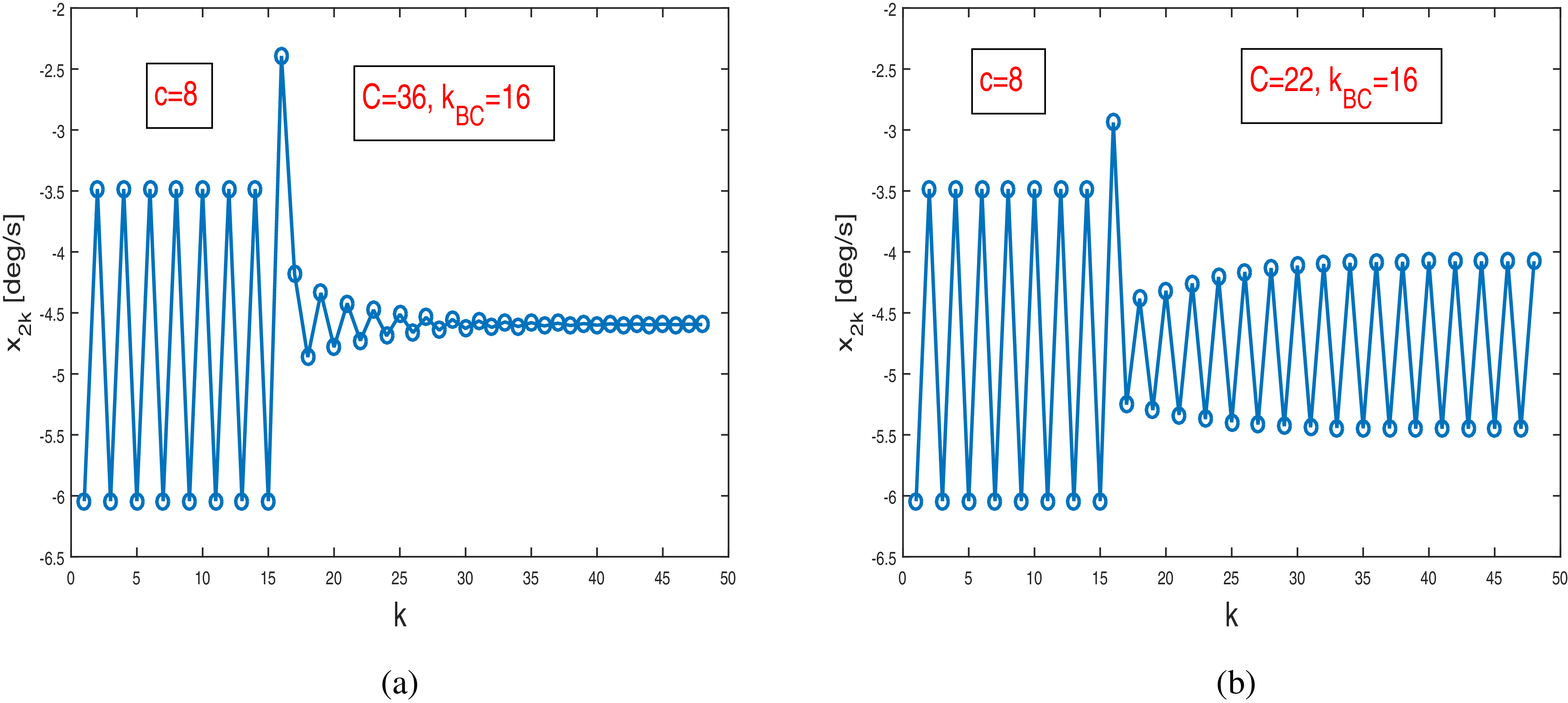
to the robot from step 16, The period-
 $2$
gait can be gradually controlled to a period-
 $1$
gait in Figure 8(a). Figure 8(b) shows that if
 $C=22\notin (27.6641,\ 82.6164)$
, the period-
 $2$
gait cannot be controlled to period-
 $1$
gait by adding the controlling pulse thrust
 $\bar {P}=12(x_2(t)^-)^2+65 x_2(t)^- +22$
.
For system (2) with
 $a=12$
,
 $c=8$
,
 $b=65$
, time series of
 $x_{2k}$
under the BC methods: (a)
 $\bar {P}=12(x_2(t)^-)^2+65 x_2(t)^- +36$
and (b)
 $\bar {P}=12(x_2(t)^-)^2+65 x_2(t)^- +22$
, which start from step 16.

Figure 8 Long description
The image contains two line graphs side by side, labeled (a) and (b), which compare gait stability analysis for bipedal robots under different boundary conditions. Both graphs plot the time series of x subscript 2k against the variable k, ranging from 0 to 50. The y-axis represents the values of x subscript 2k in degrees per second, ranging from -6.5 to -2. The first graph (a) shows data for the boundary condition method with parameters a equals 12, c equals 8, b equals 65, and P bar equals 12 times (x subscript 2(t) minus) squared plus 65 times x subscript 2(t) minus plus 36. The second graph (b) shows data for the boundary condition method with parameters a equals 12, c equals 8, b equals 65, and P bar equals 12 times (x subscript 2(t) minus) squared plus 65 times x subscript 2(t) minus plus 22. Both graphs start from step 16. The data series in both graphs exhibit oscillatory behavior with varying amplitudes and frequencies. The first graph shows a significant peak around k equals 15, while the second graph shows a more consistent oscillatory pattern throughout the range. The graphs illustrate how different boundary conditions affect the stability of the gait over time.
For system (2) with
 $a=12$
,
 $c=8$
, (a)
 $b=69$
,
 $\bar {P}=12(x_2(t)^-)^2+69 x_2(t)^- +46$
,
 $k_{BC}=26$
and (b)
 $b=70.5$
,
 $\bar {P}=12(x_2(t)^-)^2+70.5 x_2(t)^- +50$
,
 $k_{BC}=71$
, time series of
 $x_{2k}$
.

Figure 9 Long description
The image contains two line graphs side by side, each representing the time series of x2k for different gait stability parameters in bipedal robots. The left graph (a) shows data for b equals 69, c equals 8, with a specific polynomial function and kBC equals 26. The right graph (b) shows data for b equals 70.5, c equals 8, with a different polynomial function and kBC equals 71. Both graphs illustrate transitions between different gait patterns, labeled as P-4 gait and P-1 gait. The x-axis represents the variable k, and the y-axis represents x2k in degrees per second. The graphs highlight how changes in parameters affect the stability and behavior of the gait over time.
A detailed theoretical analysis for period-4 and period-8 gait control is omitted here due to its high complexity, and the numerical validations are provided in Figure 9.
5. Control of the parameter range of stable period-1 gait
A larger parameters range of one stable period-
 $1$
gait implies that this periodic motion pattern can maintain stability under a broader range of external conditions. This property enhances the disturbance rejection capability of robotic walking and simplifies the design of the walking controller. This section addresses the control over the parameter range of stable period-1 gaits. Let
 $L(c)$
denote the length of the parameter interval of the stable period-1 gait under the action of pulse thrust
 $P=a(x_2(t)^-)^2+b x_2(t)^- +c$
.
When
 $a\gt 0$
and
 $c\geq 0$
, there exists a stable period-
 $1$
gait of (2) for
 $b\in (b_1,\ b_2)$
under the pulse thrust
 $P$
, where
 $b_1,$
and
 $b_2$
are shown in (5) and (7), respectively. Hence, the pre-control length
 $L(C)$
is given as follows:
 \begin{equation} L(c)=b_2- b_1=\frac {2\sqrt {1+A^2ac}-2A \sqrt {ac}}{A}. \end{equation}
Figure 3 shows that no period-
 $1$
gait exists for
 $b\lt b_1$
; however, a stable positive fixed point of the Poincaré map (3) persists on certain intervals to the left of
 $b=b_1$
. Here, we attempt to extend the parameter interval of stable period-
 $1$
gait by applying the controlling pulse thrust
 $\bar {P}=a(x_2(t)^-)^2+b x_2(t)^- +C$
, where
 $a\gt 0$
. The corresponding length of the parameter interval for stable period-1 gait after control is denoted as
 $\bar {L}(C)$
.
When
 $a\gt 0$
and
 $C\geq 0$
, the post-control length
 $\bar {L}(C)$
is obtained:
 \begin{equation} \bar {L}(C)=\bar {b}_2- \bar {b}_1=\frac {2\sqrt {1+A^2aC}-2A \sqrt {aC}}{A}, \end{equation}
where
 $\bar {b}_1$
and
 $\bar {b}_2$
are given in Subsection 3.2. In view of (16),
 \begin{equation*} \frac {\textrm {d} \bar {L}(C) }{\textrm {d} C }=a \left (\frac {A}{\sqrt {1+A^2aC}}-\frac {1}{\sqrt {aC}}\right )\lt 0. \end{equation*}
Then the post-control length
 $\bar {L}(C)$
decreases with the controlling pulse thrust parameter
 $C$
increasing, which theoretically verifies the fact observed in Figure 5. The following result is obtained:
 \begin{equation} \bar {L}(C) \gt L(c),\ \ \textrm {for }\ \ C\in (0,\ c). \end{equation}
At
 $C\geq 0$
, the maximum
 $\bar {L}(C)$
is
 \begin{equation} \lim _{C \to 0^+} \bar {L}(C)=\frac {2}{A}. \end{equation}
When
 $a\gt 0$
and
 $C\lt 0$
, the Poincaré map (3) has one negative fixed point and one positive fixed point:
 \begin{equation*}\left \{ {\begin{array}{*{20}{c}} \bar {y}_{ 0 1} = \dfrac {-(Ab+\cos \gamma -1)- \sqrt {\bar {\Delta }_1 }}{2Aa}\lt 0,\\[6pt] \bar {y}_{ 0 2} =\dfrac {-(Ab+\cos \gamma -1)+ \sqrt {\bar {\Delta }_1 }}{2Aa}\gt 0, \end{array}} \right . \end{equation*}
where
 $\bar {\Delta }_1= (Ab+\cos \gamma -1)^2-4A^2aC$
. The eigenvalue of the fixed point
 $ \bar {y}_{ 0 1}$
is
 \begin{equation*} \bar {\lambda }_{01}=1-\sqrt {(Ab+\cos \gamma -1)^2-4A^2aC }. \end{equation*}
For
 $b\in (\bar {b}_3,\ \bar {b}_2)$
and
 $-\frac {1}{A^2a}\lt C\lt 0$
,
 $|\bar {\lambda }_{01}|\lt 1$
and the fixed point
 $\bar {y}_{ 0 1}$
is stable; hence, there is a stable period-
 $1$
gait, where
 \begin{equation} \bar {b}_2=\frac {2\sqrt {1+A^2aC}+1-\cos \gamma }{A},\ \bar {b}_3=\frac {-2\sqrt {1+A^2aC}+1-\cos \gamma }{A}. \end{equation}
Thus, the post-control length
 $\bar {L}(C)$
is obtained for
 $a\gt 0$
and
 $C\lt 0$
:
 \begin{equation} \bar {L}(C)=\bar {b}_2- \bar {b}_3=\frac {4\sqrt {1+A^2aC}}{A}. \end{equation}
It follows that
 $\frac {\textrm {d} \bar {L}(C) }{\textrm {d} C }=\frac {2Aa}{\sqrt {1+A^2aC}}\gt 0$
, which means that the post-control length
 $\bar {L}(C)$
increases with the controlling pulse thrust parameter
 $C$
increasing, where
 $-\frac {1}{A^2a}\lt C\lt 0$
. The maximum
 $\bar {L}(C)$
is
 \begin{equation} \lim _{C \to 0^-} \bar {L}(C)=\frac {4}{A}. \end{equation}
Assume that
 $\bar {L}(C)= L(c)$
. In view of (15) and (20),
 \begin{equation*} \frac {2\sqrt {1+A^2ac}-2A \sqrt {ac}}{A}=\frac {4\sqrt {1+A^2aC}}{A}, \end{equation*}
which solution is
 \begin{equation} C=\frac {(\sqrt {1+A^2ac}-A \sqrt {ac} )^2 -4}{4A^2a} =C_0. \end{equation}
Therefore, the following result is obtained:
 \begin{equation} \bar {L}(C) \gt L(c),\ \ \textrm {for }\ \ C\in (C_0,\ 0). \end{equation}
In view of (17) and (23), the result about control of parameter range of stable period-1 gaits is given as follows.
Proposition 4.
Let
 $L(c)$
be the length of parameter interval of the stable period-
 $1$
gait of (
2
) under the pulse thrust
 $P=a(x_2(t)^-)^2+b x_2(t)^- +c$
with
 $a\gt 0$
and
 $c\geq 0$
. To extend the stable parameter interval, the controlling pulse thrust
 $\bar {P}=a(x_2(t)^-)^2+b x_2(t)^- +C$
is added to the robot. The post-control length
 $\bar {L}(C)$
is larger than the pre-control length
 $L(c)$
for
 $C_0\lt C\lt c$
, where
 $C_0$
is shown in (
22
).
The length of the stable parameter interval
 $\bar {L}(C)$
under the controlling pulse thrust
 $\bar {P}=12(x_2(t)^-)^2+b x_2(t)^- +C$
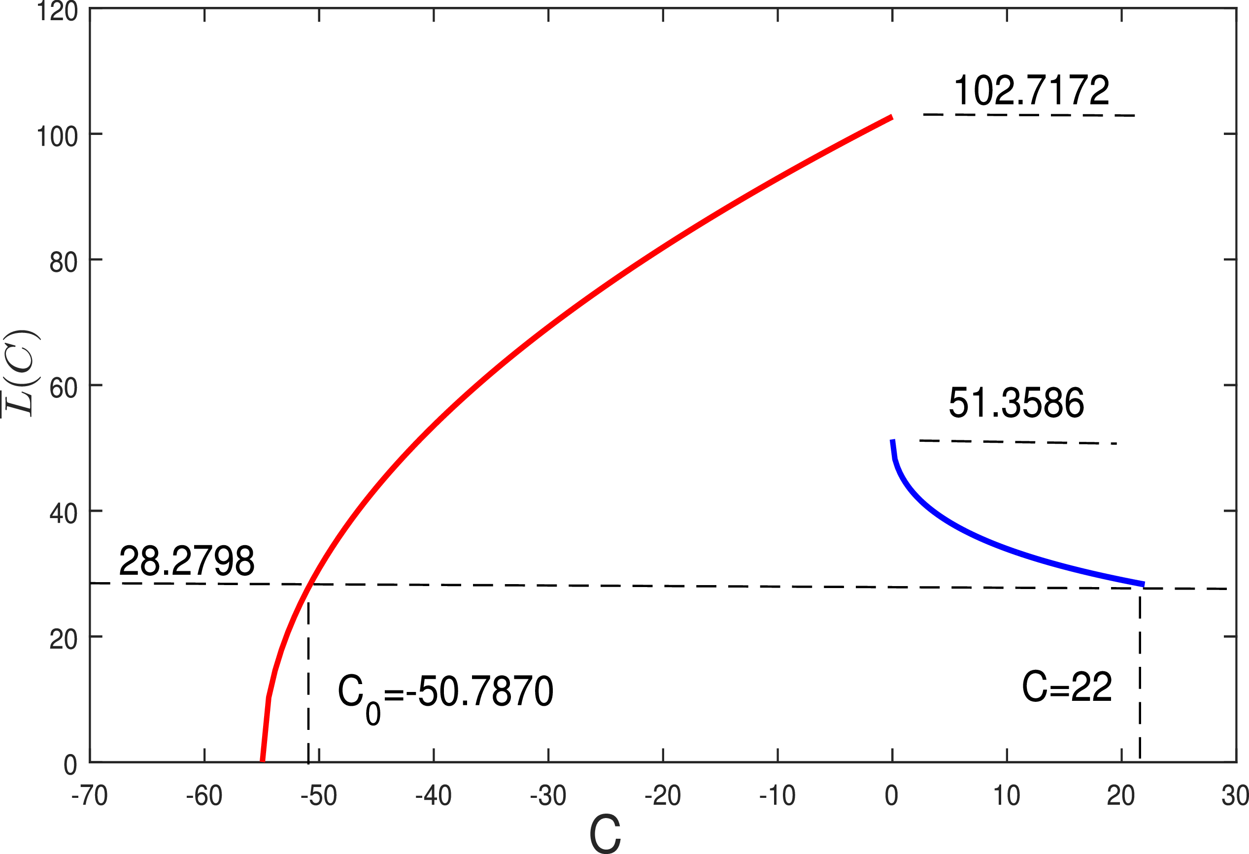
.

Figure 10 Long description
A line graph showing the length of the stable parameter interval L bar C under the controlling pulse thrust P bar equals 12 times x 2 t minus squared plus b times x 2 t minus plus C. The x axis represents the parameter C ranging from negative 70 to 30. The y axis represents the length of the stable parameter interval L bar C ranging from 0 to 120. The graph features two distinct curves: a red curve that starts at C 0 equals negative 50.7870 and rises steeply to a value of 102.7172, and a blue curve that starts at C equals 22 and descends to a value of 51.3586. The red curve indicates a positive relationship between C and L bar C, while the blue curve shows a negative relationship. All values are approximated.
Proposition4 provides the theoretical framework for increasing the pre-control length
 $L(c)$
, which is demonstrated by numerical results through the following example.
For a case study with
 $a=12$
and
 $c=22$
, the pre-control length is
 $L(22)=28.2798$
(derived from (15)). In view of (18), (21), and (22), one can calculate that
 \begin{equation*} L(0^+)=51.3586,\ \ L(0^-)=102.7172,\ \ C_0=-50.7870. \end{equation*}
Hence, the post-control length
 $\bar {L}(C)\gt L(22)$
for
 $C\in (\!-50.7870,\ 22)$
, which is shown in Figure 10.
The numerical results about the post-control length
 $\bar {L}(C)$
with
 $C= -6,\ 0^+,\ 0.22$
are shown in Figure 11. In these three cases, the post-control lengths
 $\bar {L}(C)$
are all greater than
 $L(22)=28.2798$
. However, for
 $C=-51.2\notin (\!-50.7870,\ 22)$
,
 $\bar {L}(\!-51.2)=26.8411\lt L(22)$
, which is shown in Figure 11(d).
The numerical results in Figure 11 can also serve as a reference for configuring the controller. For example, in Figure 11(c),
 $C=-6$
, the stable parameter interval for the period-
 $1$
gait is
 $(\!-46.4467,\ 50.5009)$
with an interval length of 96.9476 far exceeding
 $L(22)$
. However, when
 $b=-40\in (-46.4467,\ 50.5009)$
, the fixed point is
 $\bar {y}_{01}=-0.1431$
, meaning the velocity
 $\dot \theta _{s}=-0.1431$
. Depending on whether this angular velocity meets the practical requirements for velocity, it can be determined whether to exclude
 $b=-40$
during controller configuration.
Stable parameter interval and its length for the period-
 $1$
gait under the controlling pulse thrust
 $\bar {P}=12(x_2(t)^-)^2+b x_2(t)^- +C$
with (a)
 $C=0.22$
, (b)
 $C= 0^+$
, (c)
 $C= -6$
, and (d)
 $C= -51.2$
.

Figure 11 Long description
The image contains four separate graphs labeled (a), (b), (c), and (d), each depicting stable parameter intervals for the period-1 gait under different controlling pulse thrusts. The x-axis represents the parameter b, while the y-axis represents x subscript 2k. Each graph shows different values of C: (a) C equals 0.22, (b) C equals 0 positive, (c) C equals negative 6, and (d) C equals negative 51.2. The graphs use red and blue colors to indicate different regions of stability. The red regions represent unstable areas, while the blue regions represent stable areas. Each graph also includes specific values marked with dashed lines, indicating critical points or thresholds within the parameter space. The graphs illustrate how changes in the controlling pulse thrust affect the stability of the gait.
6. Conclusion
Aiming at the research gaps of existing studies (lack of systematic research on impulse-driven bipedal robots, poor practicality of control methods, and no quantitative analysis on stability domain expansion), this study investigates the gait control of impulse-driven bipedal robots, and its distinct contributions are as follows: a practical bifurcation control method and explicit quantitative design boundaries for period-1 gait stable parameters. These contributions complement the bipedal robot gait control research system and provide feasible guidance for practical engineering applications.
Both the OC and BC methods can stabilize chaotic gaits to stable period-1 gaits, with distinct trade-offs in energy consumption and implementation complexity. OGY control consumes less energy but relies on real-time trajectory monitoring and has the risk of control interruption. Bifurcation control achieves timely control through constant thrust increments and is simple to design, making it more suitable for practical robot applications and thus preferentially recommended for chaotic gait stabilization.
By adjusting the parameter
 $C$
of pulse thrust through bifurcation control, multi-period gaits (period-2, 4, 8, etc.) can be successfully converted into stable period-
 $1$
gaits within a specific interval (
 $c_1 \lt C\lt c_2$
). This solves the problems of high computational complexity and difficulty in implementing multi-period gaits, improving the stability and efficiency of the robot’s gait.
The stable parameter range of the period-
 $1$
gait can be significantly expanded by optimizing the pulse thrust parameter
 $C$
. When
 $C$
is within
 $(C_0,\ c)$
(where
 $C_0$
is the critical value), the post-control stable range length
 $\bar {L}(C)$
is greater than the pre-control length
 $L(c)$
. Especially when
 $C\lt 0$
and close to 0, the length of the stable interval can reach several times that before control (e.g., from 28.28 to 102.72), greatly enhancing the robot’s robustness to parameter changes and external disturbances.
The impulse-driven control strategy proposed in this paper provides a systematic solution for the stable walking of bipedal robots. Its conclusions are verified through numerical simulations and can guide the controller design of practical bipedal robots. The phase-plane trajectories and plots of the system response, added to the analysis of OGY and bifurcation control effects, further deepen the insight into the dynamic behavior of the bipedal robot system under impulsive actuation and strengthen the discussion on the stability of the controlled period-1 gait, in line with the conventional analysis standards for biped robotic system dynamics.
While this study provides a comprehensive theoretical framework and numerical validation for impulsive gait control, we acknowledge that experimental implementation would be necessary to fully assess practical performance. The proposed bifurcation control scheme, which is implemented via constant thrust increments, is deliberately designed for hardware feasibility, as it requires only adjustment of a single parameter
 $C$
and does not demand high-frequency state measurements. Experimental realization would involve integrating force/torque sensors for heel-strike detection and employing programmable actuators or spring-loaded mechanisms to generate the prescribed pulse thrust.
The bifurcation control method proposed in this study alters the dynamic behavior by adjusting parameters of the simplified system, guiding it from chaotic states to stable periodic orbits. Relying on precise system modeling and bifurcation analysis, it can ensure stability within analytically derived stable parameter ranges. This approach is particularly suitable for applications with limited computational resources or where certifiable stability guarantees are required. In contrast, the neural network-based adaptive predictive feedback control approach [Reference Zhang, Zhou, Wang, Liu and Wu27], which is one of the contemporary control methods, leverages neural networks to learn system nonlinearities online and integrate predictive models to achieve data-driven adaptive control, offering stronger robustness and environmental adaptability. However, this control approach typically requires extensive training data, substantial computational resources and may lack interpretability.
The bipedal robot walking model established in Section 2 is based on two classic simplifying assumptions: massless rigid legs and a point-mass hip. This simplified model aims to reveal the essential characteristics of gait dynamics under impulsive actuation and to provide a clear analytical framework for proposing control strategies. In practical biomimetic bipedal robot systems, leg inertia, mass distribution, and the compliance of joints and structures can influence gait stability and control performance.
Considering distributed leg mass increases the total rotational inertia of the system, prolongs the gait cycle, and slows down dynamic response. It also shifts the overall center of mass from the hip toward the legs, affecting gravitational torque during stance and potentially necessitating adjustments to the pulse thrust parameters for optimal efficiency. Leg inertia alters angular momentum transfer during foot–ground contact, extends the natural oscillation period, and may modify the optimal step cycle period. Compliance absorbs impact energy, reduces impact forces during foot contact, introduces additional vibrational modes that could lead to higher-order bifurcations, and modifies energy efficiency.
The aforementioned factors alter the walking dynamics of bipedal robots. For instance, the values of stability boundaries
 $b_1$
(6) and
 $b_2$
(7) change, the fixed-point position
 $y_{01}$
of periodic gait shifts, the locations of bifurcation points and the boundaries of chaotic regions move, and new instability modes may emerge in previously stable periodic gaits. These factors also present more complex challenges for the control system. In pulse thrust control, compliance may play a dual role: on the one hand, it cushions the control pulse; on the other hand, it introduces phase delays that could reduce control response speed.
Parameter
 $A=\frac { \sin \gamma }{lM}$
plays a crucial role in determining system dynamics, as evident in (3), (6), and (7). Now provide a sensitivity analysis of parameter
 $A$
under the simplified model. In view of (6), (7), and (15),
 \begin{equation*} \frac {L(c)}{\partial A}=\frac {\partial (b_2-b_1)}{\partial A}=-\frac {2}{A^2 \sqrt {1+A^2ac}}\lt 0. \end{equation*}
Thus, increases in both leg length
 $l$
and mass
 $M$
lead to a decrease in parameter
 $A$
, which in turn causes the stability interval
 $(b_1,\ b_2)$
of period-
 $1$
gait to widen. Table II shows the impact of changes in parameter
 $A$
on the stability boundaries by using the nominal values
 $a=12$
,
 $c=8$
,
 $\gamma =0.4rad$
, and
 $A=0.0389$
(corresponding to typical parameters:
 $l=1 m$
,
 $M=10 kg$
).
From Table II, it can be observed that although the model assumes massless legs and a point-mass hip (Section 2), the control strategy proposed in this paper exhibits a certain degree of robustness to variations in model parameters.
The current study is based on a simplified 2-DOF bipedal robot model with leg mass concentrated at the hip joint, which captures the essential swing-stance dynamics and impulsive actuation mechanism while maintaining analytical tractability. The control of the robot’s walking gaits is discussed through the analysis of a one-dimensional map. However, several challenges are presented by the extension of the proposed modeling and control framework to higher-DOF humanoid systems (e.g., those with articulated knees, ankles, and a torso). First, the dimensionality of the state space increases significantly, leading to a more complex Poincaré that may not admit a closed-form expression. Second, additional degrees of freedom introduce coupling effects and multiple impact events, which could give rise to new bifurcation phenomena and more intricate gait patterns.
Despite these complexities, the core ideas – such as pulse thrust parameterization, bifurcation analysis, and OGY/bifurcation control – are conceptually scalable, and for higher-DOF systems, numerical methods (e.g., data-driven Poincaré map identification or machine learning-based control) could complement the analytical approach presented here. Future research will develop more refined dynamic models that fully account for the mass distribution, moment of inertia and structural flexibility of the legs, the high-order coupling effects under high-speed motion, and the complex scenarios involving multiple pulse torques per step. The gait stability and gait control of bipedal robots will be further investigated by utilizing the obtained multidimensional maps as well as their fixed points and entire spectrum of Lyapunov exponents. A promising future direction is also to combine the proposed impulse-based control strategy with whole-body control frameworks (e.g., model predictive control or hierarchical optimization) to achieve stable and efficient walking in full-scale humanoid robots, which would allow experimental validation on physical platforms and bridge the gap between theoretical analysis and practical deployment.
Sensitivity analysis of parameter
 $A$
.

Table II Long description
The table presents the sensitivity analysis of parameter A on the stability boundaries of a system, focusing on variations in leg length l and mass M. It consists of four rows and four columns. The columns are labeled Parameter variation, A, b1, b2, and Effect on L(c). The rows detail the baseline values and the effects of increasing leg length by 9 percent and mass by 20 percent. For the baseline with l equals 1 meter and M equals 10 kilograms, A is 0.0389, b1 is 21.6230, b2 is 56.9972, and the effect on L(c) is 35.3742. When l increases by 9 percent, A becomes 0.0354, b1 is 21.8258, b2 is 59.0701, and the effect on L(c) increases by 5.29 percent to 37.2443. When M increases by 20 percent, A is 0.0325, b1 is 22.0285, b2 is 64.3800, and the effect on L(c) increases by 19.72 percent to 42.3515. The table highlights how increases in leg length and mass lead to a decrease in parameter A, which widens the stability interval (b1, b2) of period-1 gait.
Author contributions
Tengfei Long and Guirong Jiang conceived and designed the study. Tengfei Long conducted investigation and formal analysis. Guirong Jiang and Tengfei Long wrote the article.
Financial support
This work is supported by the National Natural Science Foundation of China (12271119 and 11662001).
Competing interests
The authors declare no conflict of interest.
Data availability
Data sharing is not applicable to this article as no data were used for the research described in the study.

 u1
 u2
 u
 P

 b
 a=12
 c=8

 a=12
 c=8
 b
 b

 a=12
 c=8
 b=b0=73
 σ=0.9
 kOC=16
 x2k
 1
 x1(x3)
 x2(x4)
 x2
 deg/s

 b
 P=a(x2(t)−)2+bx2(t)−+c (a=12, c=8)
 P¯=a(x2(t)−)2+bx2(t)−+C (a=12, C=52)

 a=12
 c=8
 b=b0=73
 P¯=12(x2(t)−)2+73x2(t)−+52
 kBC=16
 x2k
 1
 x1(x3)
 x2(x4)
 x2
 deg/s

 P¯−P

 a=12
 c=8
 b=b0=73
 x2k
 a=12
 c=8
 b=65
 x2k
 P¯=12(x2(t)−)2+65x2(t)−+36
 P¯=12(x2(t)−)2+65x2(t)−+22

 a=12
 c=8
 b=69
 P¯=12(x2(t)−)2+69x2(t)−+46
 kBC=26
 b=70.5
 P¯=12(x2(t)−)2+70.5x2(t)−+50
 kBC=71
 x2k
 L¯(C)
 P¯=12(x2(t)−)2+bx2(t)−+C

 1
 P¯=12(x2(t)−)2+bx2(t)−+C
 C=0.22
 C=0+
 C=−6
 C=−51.2

 A


