2.1 The viscous/inviscid interaction (VII) method

In the panel method, the total flow velocity $\boldsymbol{q}$ is decomposed into an incoming flow $\boldsymbol{q}_{in}$ and a propeller-induced flow $\boldsymbol{U}_{ind}$ (the perturbation velocity),

(2.1) $$\begin{eqnarray}\displaystyle \boldsymbol{q}=\boldsymbol{q}_{in}+\boldsymbol{U}_{ind}. & & \displaystyle\end{eqnarray}$$

$\boldsymbol{U}_{ind}$ can be treated as the potential flow which is governed by the Laplace equation

(2.2a,b ) $$\begin{eqnarray}\displaystyle \boldsymbol{U}_{ind}=\unicode[STIX]{x1D735}\unicode[STIX]{x1D719},\quad \unicode[STIX]{x1D6FB}^{2}\unicode[STIX]{x1D719}=0, & & \displaystyle\end{eqnarray}$$

where $\unicode[STIX]{x1D719}$ is the perturbation potential.

The Kutta condition is required which means the velocity must remain finite

(2.3) $$\begin{eqnarray}\displaystyle |\unicode[STIX]{x1D735}\unicode[STIX]{x1D719}|<\infty \quad \text{at the trailing edge.} & & \displaystyle\end{eqnarray}$$

By using Green’s identity, equation (2.2) can be written in the boundary integrated form:

(2.4) $$\begin{eqnarray}\displaystyle 2\unicode[STIX]{x03C0}\unicode[STIX]{x1D719}_{p}=\iint _{S_{H}}\left[\unicode[STIX]{x1D719}_{p}\frac{\unicode[STIX]{x2202}G(p,p^{\prime })}{\unicode[STIX]{x2202}\boldsymbol{n}_{p^{\prime }}}-G(p,p^{\prime })\frac{\unicode[STIX]{x2202}\unicode[STIX]{x1D719}_{p}}{\unicode[STIX]{x2202}\boldsymbol{n}_{p^{\prime }}}\right]\text{d}S+\iint _{S_{W}}\unicode[STIX]{x0394}\unicode[STIX]{x1D719}_{W}\frac{\unicode[STIX]{x2202}G(p,p^{\prime })}{\unicode[STIX]{x2202}\boldsymbol{n}_{p^{\prime }}}\,\text{d}S, & & \displaystyle\end{eqnarray}$$

where $S_{H}$ is the surface of the hydrofoil or propeller blade, duct and hub, $S_{W}$ the surface of the trailing wake, $G$ Green’s function, which is defined as $1/R(p,p^{\prime })$ in three dimensions and $2lnR(p,p^{\prime })$ in two dimensions and $R$ the distance between the two points $p$ and $p^{\prime }$ .

The panel method is based on potential theory, which is inviscid. The effect of viscosity can be taken into account by placing boundary layer sources on the surfaces $S_{H}$ and $S_{W}$ , which is known as the viscous/inviscid interaction method. The edge velocity of the boundary layer is from solving the potential flow by using the panel method. The strength of the boundary layer sources can be obtained from a boundary layer solver (Drela Reference Drela1989) and the viscous velocity on the $i$ th panel is obtained by

(2.5) $$\begin{eqnarray}\displaystyle \boldsymbol{U}_{i,vis}=\boldsymbol{U}_{i,ind}+\mathop{\sum }_{j=1}^{N+N_{W}}\unicode[STIX]{x1D60A}_{ij}\unicode[STIX]{x1D70E}_{j}, & & \displaystyle\end{eqnarray}$$

where $\boldsymbol{U}_{i,ind}$ is the edge velocity on the $i$ th panel, $N$ and $N_{W}$ the number of panels on $S_{H}$ and $S_{W}$ , $\unicode[STIX]{x1D60A}_{ij}$ the source influence coefficient matrix and $\unicode[STIX]{x1D70E}_{j}$ the boundary layer source strength on the $j$ th panel.

Drela’s (Reference Drela1989) model can predict the transition points from the laminar flow to turbulent flow on both the pressure side and the suction side. However, in the presented method, the flow is assumed to be fully turbulent. Forced transitions at $1\,\%$ chord length from the leading edge are applied in the VII method throughout this study, and results are compared with fully turbulent RANS simulations.

2.2 The extension model

An extension model is needed for sections with blunt TEs because the viscous/inviscid interaction method only applies to sections with sharp TEs. Physically, the extension represents the separated flow downstream of the blunt TE, which is built by quadratic curves to guarantee that both the geometry and the slope are continuous at points A and B, as shown in figure 1. If the coordinates of points A, B and C are given, the extension is uniquely determined by solving the equation set

(2.6) $$\begin{eqnarray}\displaystyle \left.\begin{array}{@{}l@{}}y_{C}=a_{1}x_{C}^{2}+b_{1}x_{C}+c_{1}\\ y_{A}=a_{1}x_{A}^{2}+b_{1}x_{A}+c_{1}\\ \text{slope}_{A}=2a_{1}x_{A}+b_{1}\\ y_{C}=a_{2}x_{C}^{2}+b_{2}x_{C}+c_{2}\\ y_{B}=a_{2}x_{B}^{2}+b_{2}x_{B}+c_{2}\\ \text{slope}_{B}=2a_{2}x_{B}+b_{2}\end{array}\right\}, & & \displaystyle\end{eqnarray}$$

where $x_{A}$ , $y_{A}$ , $x_{B}$ , $y_{B}$ , $x_{C}$ and $y_{C}$ are coordinates of points A, B and C, and $\text{slope}_{A}$ and $\text{slope}_{B}$ are known from the original section. The other parameters are the coefficients of the quadratic function and need to be solved.

Figure 1.

A hydrofoil and a duct with blunt TEs, which have been extended to the sharp TEs (points A and B: location where the extended section merges with the original section; point C: TE of the extended section; point M: TE of the original section; $l_{i}$ : the moment arm from point M to the lift going through the control point of panel $i$ ; $\text{d}l_{i}$ : horizontal length of panel $i$ ; $p_{i}$ : pressure at the control point; $r_{i}$ : radius at the control point; $\unicode[STIX]{x1D6FC}$ : angle of attack, exaggerated).

Equation (2.6) can be written in the rotational invariant form by replacing $x$ and $y$ in the polynomial functions with $r(\unicode[STIX]{x1D703})$ functions in a polar coordinate system centred around point C. In this case $c_{1}=c_{2}=0$ and (2.6) can be simplified as

(2.7) $$\begin{eqnarray}\displaystyle \left.\begin{array}{@{}l@{}}\displaystyle \sin (\unicode[STIX]{x1D703}_{A})=a_{1}r_{A}\cos ^{2}(\unicode[STIX]{x1D703}_{A})+b_{1}\cos (\unicode[STIX]{x1D703}_{A})\\ \displaystyle \left.\frac{\text{d}r}{\text{d}\unicode[STIX]{x1D703}}\right|_{A}=\frac{\sin ^{2}(\unicode[STIX]{x1D703}_{A})+1-b_{1}\sin (\unicode[STIX]{x1D703}_{A})\cos (\unicode[STIX]{x1D703}_{A})}{a_{1}\cos ^{3}(\unicode[STIX]{x1D703}_{A})}\\ \displaystyle \sin (\unicode[STIX]{x1D703}_{B})=a_{2}r_{B}\cos ^{2}(\unicode[STIX]{x1D703}_{B})+b_{2}\cos (\unicode[STIX]{x1D703}_{B})\\ \displaystyle \left.\frac{\text{d}r}{\text{d}\unicode[STIX]{x1D703}}\right|_{B}=\frac{\sin ^{2}(\unicode[STIX]{x1D703}_{B})+1-b_{2}\sin (\unicode[STIX]{x1D703}_{B})\cos (\unicode[STIX]{x1D703}_{B})}{a_{2}\cos ^{3}(\unicode[STIX]{x1D703}_{B})}\end{array}\right\}, & & \displaystyle\end{eqnarray}$$

where $r_{A}$ , $r_{B}$ , $\unicode[STIX]{x1D703}_{A}$ and $\unicode[STIX]{x1D703}_{B}$ are known for given points A and B, $\text{d}r/\text{d}\unicode[STIX]{x1D703}|_{A}$ and $\text{d}r/\text{d}\unicode[STIX]{x1D703}|_{B}$ from the original geometry.

Points A, B and C are determined in two loops, as shown in the flowchart in figure 2. In the outer loop, an interactive algorithm is used to move points A and B along the surface of the original section until they overlap with the flow separation points, where the skin friction becomes equal to zero with a certain tolerance. In the inner loop, point C is moved in both the horizontal and vertical directions (or in the axial and radial directions for the duct case) by using a two-dimensional Newton–Raphson method. Since there are two unknowns, $x_{C}$ and $y_{C}$ , two equations are needed. It is assumed that the pressure is constant in the separated region downstream of the blunt TE, so the force of the extension in the direction perpendicular to the inflow is zero, yielding a zero lift criterion. Similarly, a zero moment criterion requires that the moment around the original TE (point M) is zero, which gives the second equation, as shown in

(2.8) $$\begin{eqnarray}\displaystyle \left.\begin{array}{@{}l@{}}\displaystyle \int _{S_{E}}p(x)\,\text{d}A=0\\ \displaystyle \int _{S_{E}}p(x)l(x)\,\text{d}A=0\end{array}\right\}, & & \displaystyle\end{eqnarray}$$

where $S_{E}$ is the extended surface downstream of the TE (both sides), $p(x)$ the pressure distribution on $S_{E}$ , $l(x)$ the moment arm from point M with respect to the lift and $\text{d}A$ the infinitesimal area in the inflow direction. The discretized form of (2.8) is

(2.9a ) $$\begin{eqnarray}\displaystyle \left.\begin{array}{@{}l@{}}\displaystyle \mathop{\sum }_{lower,upper}\mathop{\sum }_{i}c_{p_{i}}\times \text{d}l_{i}\times \cos (\unicode[STIX]{x1D6FC})=0\\ \displaystyle \mathop{\sum }_{lower,upper}\mathop{\sum }_{i}c_{p_{i}}\times \text{d}l_{i}\times l_{i}\times \cos (\unicode[STIX]{x1D6FC})=0\end{array}\right\} & & \displaystyle\end{eqnarray}$$

and

(2.9b ) $$\begin{eqnarray}\displaystyle \left.\begin{array}{@{}l@{}}\displaystyle \mathop{\sum }_{inner,outer}\mathop{\sum }_{i}c_{p_{i}}\times \text{d}l_{i}\times 2\unicode[STIX]{x03C0}r_{i}=0\\ \displaystyle \mathop{\sum }_{inner,outer}\mathop{\sum }_{i}c_{p_{i}}\times \text{d}l_{i}\times l_{i}\times 2\unicode[STIX]{x03C0}r_{i}=0\end{array}\right\} & & \displaystyle\end{eqnarray}$$

for hydrofoil and duct respectively, where $\unicode[STIX]{x1D6FC}$ is the angle of attack, $c_{p_{i}}$ the pressure coefficient at the control point of panel $i$ , defined as

(2.10) $$\begin{eqnarray}\displaystyle c_{p_{i}}=\frac{p_{i}-p_{\infty }}{\frac{1}{2}\unicode[STIX]{x1D70C}v_{\infty }^{2}}, & & \displaystyle\end{eqnarray}$$

with $p_{\infty }$ and $v_{\infty }$ being the pressure and velocity at far upstream respectively and $\unicode[STIX]{x1D70C}$ being the fluid density.

Figure 2.

Flowchart of the extension model.

It should be noted that shorter extensions will intrinsically make the force and moment differences between the two sides smaller, thus the Newton–Raphson method tends to converge to smaller $x_{C}$ . To avoid this drawback, when applying this model numerically, the actual equations used are normalized by setting the pressure coefficient equal to unity in (2.9b ), as

(2.11a ) $$\begin{eqnarray}\displaystyle \left.\begin{array}{@{}l@{}}\displaystyle \frac{\displaystyle \mathop{\sum }_{lower,upper}\mathop{\sum }_{i}c_{p_{i}}\times \text{d}l_{i}\times \cos (\unicode[STIX]{x1D6FC})}{\displaystyle \mathop{\sum }_{lower,upper}\mathop{\sum }_{i}\text{d}l_{i}\times \cos (\unicode[STIX]{x1D6FC})}=0\\ \displaystyle \frac{\displaystyle \mathop{\sum }_{lower,upper}\mathop{\sum }_{i}c_{p_{i}}\times \text{d}l_{i}\times l_{i}\times \cos (\unicode[STIX]{x1D6FC})}{\displaystyle \mathop{\sum }_{lower,upper}\mathop{\sum }_{i}\text{d}l_{i}\times l_{i}\times \cos (\unicode[STIX]{x1D6FC})}=0\end{array}\right\} & & \displaystyle\end{eqnarray}$$

and

(2.11b ) $$\begin{eqnarray}\displaystyle \left.\begin{array}{@{}l@{}}\displaystyle \frac{\displaystyle \mathop{\sum }_{inner,outer}\mathop{\sum }_{i}c_{p_{i}}\times \text{d}l_{i}\times 2\unicode[STIX]{x03C0}r_{i}}{\displaystyle \mathop{\sum }_{inner,outer}\mathop{\sum }_{i}\text{d}l_{i}\times 2\unicode[STIX]{x03C0}r_{i}}=0\\ \displaystyle \frac{\displaystyle \mathop{\sum }_{inner,outer}\mathop{\sum }_{i}c_{p_{i}}\times \text{d}l_{i}\times l_{i}\times 2\unicode[STIX]{x03C0}r_{i}}{\displaystyle \mathop{\sum }_{inner,outer}\mathop{\sum }_{i}\text{d}l_{i}\times l_{i}\times 2\unicode[STIX]{x03C0}r_{i}}=0\end{array}\right\}. & & \displaystyle\end{eqnarray}$$

2.3 The Reynolds-averaged Navier–Stokes (RANS) method

In the VII method, the unknown sources and dipoles are placed on the surface of the body and the wake. In the RANS method, the computational domain extends from the body to far upstream and downstream, as shown in figure 3. The velocity field $u_{i}$ is decomposed into its mean $U_{i}$ and the fluctuation $u_{i}^{\prime }$ (Reynolds Reference Reynolds1894), as

(2.12) $$\begin{eqnarray}\displaystyle u_{i}=U_{i}+u_{i}^{\prime }. & & \displaystyle\end{eqnarray}$$

The governing equations in the RANS method are the continuity equation and the momentum equations, as

(2.13) $$\begin{eqnarray}\displaystyle \unicode[STIX]{x1D735}\boldsymbol{\cdot }\boldsymbol{u}=0, & & \displaystyle\end{eqnarray}$$

and

(2.14) $$\begin{eqnarray}\displaystyle \frac{\unicode[STIX]{x2202}U_{i}}{\unicode[STIX]{x2202}t}+U_{j}\frac{\unicode[STIX]{x2202}U_{i}}{\unicode[STIX]{x2202}x_{j}}=-\frac{\unicode[STIX]{x2202}P}{\unicode[STIX]{x2202}x_{i}}+\frac{\unicode[STIX]{x2202}}{\unicode[STIX]{x2202}x_{j}}\left(\unicode[STIX]{x1D708}\frac{\unicode[STIX]{x2202}U_{i}}{\unicode[STIX]{x2202}x_{j}}-\overline{u_{i}^{\prime }u_{j}^{\prime }}\right), & & \displaystyle\end{eqnarray}$$

where $P$ is the pressure, $\unicode[STIX]{x1D708}$ the kinematic viscosity and $\overline{u_{i}^{\prime }u_{j}^{\prime }}$ the Reynolds stress.

In this study, the results from the flow separation model will be compared with the RANS simulation by using the commercial computational fluid dynamics (CFD) software Ansys-Fluent. The flow is assumed to be incompressible and fully turbulent. At high Reynolds number, there might be vortex shedding after blunt trailing edges, which cannot be predicted by the presented flow separation model and the VII method. However, the focus of this approach is not about the periodic unsteadiness of the vortex shedding, but about the mean pressure and forces on hydrofoils and ducts. Consequently, results from the presented method are compared with the steady RANS simulation, neglecting any vortex shedding. On the other hand, for sections shown in figure 1, the vortex shedding is not strong and its effect is local near the trailing edge, as shown in later sections. The cases with strong vortex shedding and flow separation are beyond the scope of the presented method. In the RANS simulations, the $k-\unicode[STIX]{x1D714}~SST$ model (Pope Reference Pope2000) at fully turbulent condition is used, where $k$ is the turbulent kinetic energy, $\unicode[STIX]{x1D714}$ is the specific dissipation rate and $SST$ is short for the shear stress transport. The detailed numerical settings are listed in table 1. The far-field boundary conditions are velocity inlet and pressure outlet. To make sure that perturbations caused by the foil and duct are not affected by the boundary, the velocity inlet boundaries are 50 times the chord length away from the foil or duct, and the pressure outlet boundaries are 100 times the chord length away, as shown in figure 3.

Figure 3.

The computational domain and boundary conditions in the RANS simulations.

Table 1.

Numerical settings in Ansys-Fluent simulations.

3.1 The viscous/inviscid interaction method

In this section, the results from VII are validated with those from the RANS method at fully turbulent conditions of both a hydrofoil and a bare duct with sharp TEs. The validation is necessary because the extension is determined from the pressure coefficients and skin friction. In the VII method, the transition locations are forced at $1\,\%$ of the chord length from the leading edge. The hydrofoil, as shown in figure 4, has a NACA 0005 thickness distribution and a NACA a $=$ 0.8 mean line with the maximum camber equal to $2\,\%$ of the chord length (Abbott & Von Doenhoff Reference Abbott and Von Doenhoff1959). The angle of attack is $1.0^{\circ }$ . In the RANS simulation, the total number of quadrilateral cells is 207.6k and the wall distance $y+$ is shown in figure 5. The boundary conditions are the same as shown in figure 3(a), and other settings in the RANS simulation are shown in table 1. Compared with the panel method, the VII method improved the correlation with RANS method in pressure predictions, as shown in figure 6(a).

Figure 4.

A hydrofoil with sharp TE, tested by both VII method and the RANS simulation.

Figure 5.

Wall $y+$ in the RANS simulation for the hydrofoil with sharp TE.

Figure 6.

The pressure and skin friction predicted from VII agree well with those from RANS for hydrofoil sections with sharp TEs ( $Re=1.0\times 10^{6}$ , which is defined by the chord length $c$ as $Re=cv_{\infty }/\unicode[STIX]{x1D708}$ ; $c_{f}=\unicode[STIX]{x1D70F}_{w}/(\unicode[STIX]{x1D70C}v_{\infty }^{2})/2$ , where $\unicode[STIX]{x1D70F}_{w}$ is the wall shear stress).

The viscous drag coefficient is defined as

(3.1) $$\begin{eqnarray}\displaystyle C_{D,v}=\frac{D}{\frac{1}{2}\unicode[STIX]{x1D70C}v_{\infty }^{2}A}, & & \displaystyle\end{eqnarray}$$

where $D$ is the integrated drag force, including the pressure drag and frictional drag in the inflow direction and $A$ is the reference area, taken equal to 1 in the two-dimensional case. Drag in general, due to its small values, is hard to evaluate or to measure. The theoretical drag coefficient from the panel method, which is based on the potential theory and fully inviscid, is zero. However, this value is not always zero but a small number, which can be regarded as the numerical integration error, as shown in table 2. Considering that when $N=200$ , the drag coefficient from the panel method is two orders magnitude smaller than those from the VII method, 200 panels are used throughout the presented study in the VII method. Besides, full cosine spacing is adopted, which concentrates more panels near the leading edge and trailing edge in the VII method.

Table 2.

Viscous drag coefficients ( $C_{D,v}$ ) predicted by the panel method and the VII method with different numbers of panels ( $N$ ). Note: $C_{D,v}$ (RANS) $=$ 0.00982.

A bare duct means that the interaction between the propeller and the duct is neglected so the problem is simplified to two dimensions, and the axisymmetric sources are used in the boundary layer solver. Duct 19Am is modified from Duct 19A (Kuiper Reference Kuiper1992), which has a round TE. The model test of Duct 19Am operating with propeller Ka4-70 was carried out by Bosschers & van der Veeken (Reference Bosschers and van der Veeken2008) to provide validation data for the panel method as it generally does not apply to blunt TEs. Sections of Ducts 19A and 19Am are shown in figure 7(a).

Figure 7.

The pressure predicted from VII agrees well with that from RANS for bare duct sections with sharp TEs ( $Re=1.0\times 10^{6}$ , which is defined by the chord length of the duct $c$ as $Re=cv_{\infty }/\unicode[STIX]{x1D708}$ ; the lengths are non-dimensionalized by the blade radius $R$ ). (a) Duct section with a round TE is modified to sharp TE, (b) pressure distribution on the bare duct with a sharp TE.

In the axisymmetric RANS simulation, the total number of quadrilateral cells is 299.4 k and the $y+$ is smaller than 5 to model the viscous flow accurately in the boundary layer region. Detailed settings of the RANS simulation can be found in table 1. As shown in figures 6(a) and 7(b), the pressures predicted by the VII method agree well with those from the RANS method in sharp TE sections, and thus can be used confidently in the extension model.

3.2 Hydrofoil case with a blunt trailing edge

For the hydrofoil shown in figure 1(a), there is flow separation downstream of the blunt TE, as shown in figure 8. This geometry is originally a duct but used as a hydrofoil case in this study to test the extension model. The flow field is from the RANS simulation, in which the total number of quadrilateral cells equals 523.5 k and the $y+$ is smaller than 5. Since there is a sharp corner in the blunt TE (as opposed to round in figure 1 b and figure 7 a), the outer loop of the model is applied only on the lower side of the hydrofoil to determine the location of point B. On the upper side, since the geometry at the corner is nearly flat, it is reasonable to start the extension from that location, i.e. point A is fixed at point M. The pressures and skin frictions from the extension model with the VII method are compared with the results from the RANS method for two angles of attack (AOA), as shown in figures 9 and 10. It should be noted that, at different angles of attack, the extended geometries are not the same because the flows around the hydrofoil are different.

Figure 8.

Flow separation downstream of a hydrofoil with blunt trailing edge (plotted with zero angle of attack, $\boldsymbol{q}_{in}=1~\text{m}~\text{s}^{-1}$ at far upstream, $Re=1.0\times 10^{6}$ ; the lengths are non-dimensionalized by the hydrofoil chord length $c$ ).

Figure 9.

The pressure on a hydrofoil with a blunt trailing edge, predicted by the extension model with VII and the RANS method.

Figure 10.

The skin frictions on a hydrofoil with a blunt trailing edge, predicted by the extension model with the VII method and the RANS method.

3.3 Bare duct case with a round trailing edge

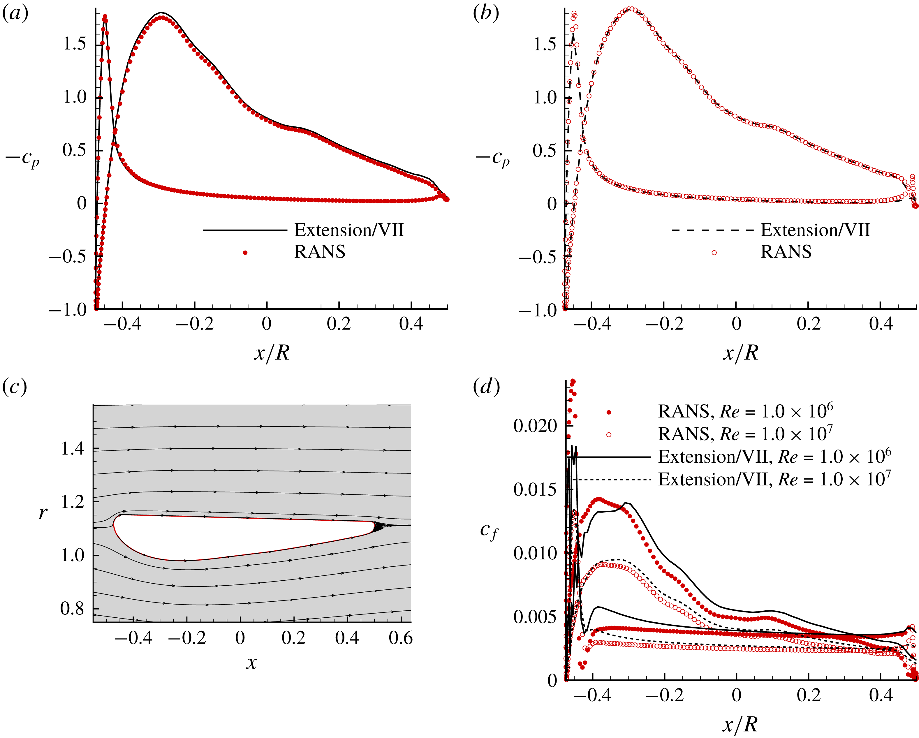
The extension model is applied to bare Duct 19A (as shown in figure 7 a) and the pressure and skin friction on the duct are compared with results from the RANS method for $Re=1.0\times 10^{6}$ and $Re=1.0\times 10^{7}$ . Since this duct geometry is built by connecting two straight lines with a round TE, the outer loop of the extension model is not applied as long as points A and B shown in figure 1 do not fall into the round TE part. A good correlation with results from the RANS method can be observed, as shown in figure 11.

Figure 11.

The extension model applied to a bare duct with a round trailing edge, and results compared with the RANS method. (a) Pressure distribution, $Re=1.0\times 10^{6}$ , (b) pressure distribution, $Re=1.0\times 10^{7}$ , (c) streamlines around the duct and the local flow separation after the round TE (predicted by the steady axisymmetric RANS method with $Re=1.0\times 10^{6}$ , (d) skin friction correlation.

Results of the extension model are compared with the steady RANS simulations and the time-averaged pressures and skin frictions are used. To check the effect of the vortex shedding, two unsteady two-dimensional axisymmetric RANS simulations are carried out with different initial conditions. The time size is set as $1.0\times 10^{-4}~\text{s}$ , based on the Courant–Friedrichs–Lewy (CFL) condition. The pressure–velocity coupling scheme is SIMPLEC, and all the other settings are the same as in table 1. In the first unsteady simulation, the flow field of the converged steady run is used as the initial condition, and by comparing the drag coefficient history with the steady simulation, it is shown that there is no vortex shedding and the drag coefficient is equal to that from the steady RANS simulation. In the second unsteady RANS run, the initial flow is set as $1~\text{m}~\text{s}^{-1}$ everywhere in the domain and the stabilized drag coefficients oscillate within a range of approximately $\pm 5\,\%$ of their mean values, which is approximately $6.8\,\%$ higher than the steady value, as shown in figure 12.

Figure 12.

Drag coefficient history from the unsteady RANS simulations with different initial conditions, compared with the steady RANS simulation ( $Re=1.0\times 10^{7}$ ).

The stabilized streamlines and vorticity are shown in figure 13. To see the effect of the vortex shedding, pressure distributions at two extreme positions in the time history and the time-averaged mean pressure over one period in the unsteady simulation are compared with those from the steady simulation, as shown in figure 14. It is found that even though the drag coefficients at certain initial conditions oscillate with time, its effect on the pressure distributions is local to the trailing edge. Hydrofoils and ducts with strong vortex shedding downstream of the blunt trailing edge cannot be handled by the presented method, therefore are not considered here.

Figure 13.

Vortex shedding downstream of a bare duct with round TE, predicted by unsteady two-dimensional axisymmetric RANS simulation ( $Re=1.0\times 10^{7}$ , $t=15.25~\text{s}$ , initial condition: $U=1~\text{m}~\text{s}^{-1}$ in the whole domain).

Figure 14.

The unsteady pressure distributions at two extreme positions in the time history and the time-averaged mean value are all close to results from the steady simulation (bare duct with round TE, $Re=1.0\times 10^{7}$ ).

The viscous drag coefficients from the presented method are compared with results from the steady RANS simulations, as shown in table 3. In figure 1, the curve between point A and point B is replaced by the extension, so $c_{p}$ and $c_{f}$ of this part are obtained by interpolation. In the bare duct case, as the Reynolds number increases, the viscous drag coefficients decrease in both methods, as expected.

Table 3.

Viscous drag coefficients ( $C_{D,v}$ ) in RANS simulations and the presented method.

3.4 Ducted propeller case with a round trailing edge

The extension model is applied to Duct 19A working with a square-tip propeller Ka4-70 with zero gap. To see the effect of the presented model, the results are compared with those from an arbitrary extension, as shown in figure 15(a). The pressure distribution along the duct when the advanced ratio equals to 0.5 is shown in figure 15(b) (averaged in the circumferential direction). The advanced ratio is defined as

(3.2) $$\begin{eqnarray}\displaystyle J=\frac{V_{s}}{nD}, & & \displaystyle\end{eqnarray}$$

where $V_{s}$ is the ship speed, $n$ the propeller rotational frequency and $D$ the propeller diameter. Note that the pressures at the TE from the arbitrary extension are not equal on both sides. However, in the case that the extension is determined by the present model, the pressures at the TE match with each other, due to the zero lift and zero moment criteria.

Figure 15.

The extension model applied to a ducted propeller with a round trailing edge duct (uniform inflow). (a) Two extensions for $J=0.5$ , one is from the model and the other is arbitrary, (b) pressure distribution on the duct from the two extensions, $J=0.5$ , (c) the open water characteristics predicted from the Extension model, arbitrary extension and the experimental measurements.

The open water characteristics of propeller Ka4-70 operating inside Duct 19A from the extension model are compared with the experimental measurements, as shown in figure 15(c). It should be noted that for different advance ratios, the length of the extension zone is not the same because the flows around the duct are different. The thrust coefficient on the propeller is defined as

(3.3) $$\begin{eqnarray}\displaystyle KTP=\frac{T_{P}}{\unicode[STIX]{x1D70C}n^{2}D^{4}}, & & \displaystyle\end{eqnarray}$$

and the thrust coefficient on the duct is defined as

(3.4) $$\begin{eqnarray}\displaystyle KTD=\frac{T_{D}}{\unicode[STIX]{x1D70C}n^{2}D^{4}}, & & \displaystyle\end{eqnarray}$$

where $T_{P}$ is the thrust on the propeller, $T_{D}$ the thrust on the duct. The torque coefficient is defined as

(3.5) $$\begin{eqnarray}\displaystyle KQ=\frac{Q}{\unicode[STIX]{x1D70C}n^{2}D^{5}}, & & \displaystyle\end{eqnarray}$$

where $Q$ is the torque on the propeller.

In figure 15(c), it can be seen that the thrust and torque agree much better with the experimental measurements when the extension zone is determined from the present model rather than by choosing random locations. It should also be noted that the duct trailing edge does not have a strong influence on the thrust from the duct, but has a strong influence on the propeller thrust and torque.

3.5 Computational efficiency of the extension model

Compared with the RANS method, this extension model does not require as many computational resources and takes a shorter time in calculation, not to mention the time for pre-processing and post-processing. An overall comparison of the computational efficiency of these two methods is shown in table 4. The RANS simulation for the ducted propeller case was done by Kinnas et al. (Reference Kinnas, Fan and Tian2015), using an Intel Xeon 2.54 GHz processor. All the other simulations were done on the clusters of the TACC (Texas Advanced Computing Center) using an Intel Xeon E5-2680 2.7 GHz processor. The residuals for all the RANS simulations were set as $1.0\times 10^{-6}$ , and only the simulation time was counted.

Table 4.

The computational efficiency of the extension model and the RANS method (only the simulation time was counted; the angle of attack is in degrees).