



%20--%3e%3c!DOCTYPE%20svg%20PUBLIC%20'-//W3C//DTD%20SVG%201.0//EN'%20'http://www.w3.org/TR/2001/REC-SVG-20010904/DTD/svg10.dtd'%3e%3csvg%20version='1.0'%20id='Layer_1'%20xmlns='http://www.w3.org/2000/svg'%20xmlns:xlink='http://www.w3.org/1999/xlink'%20x='0px'%20y='0px'%20width='64px'%20height='64px'%20viewBox='5.5%20-3.5%2064%2064'%20enable-background='new%205.5%20-3.5%2064%2064'%20xml:space='preserve'%3e%3cg%3e%3ccircle%20fill='%23FFFFFF'%20fill-opacity='0'%20cx='37.785'%20cy='28.501'%20r='28.836'/%3e%3cpath%20fill='%23595959'%20d='M37.441-3.5c8.951,0,16.572,3.125,22.857,9.372c3.008,3.009,5.295,6.448,6.857,10.314%20c1.561,3.867,2.344,7.971,2.344,12.314c0,4.381-0.773,8.486-2.314,12.313c-1.543,3.828-3.82,7.21-6.828,10.143%20c-3.123,3.085-6.666,5.448-10.629,7.086c-3.961,1.638-8.057,2.457-12.285,2.457s-8.276-0.808-12.143-2.429%20c-3.866-1.618-7.333-3.961-10.4-7.027c-3.067-3.066-5.4-6.524-7-10.372S5.5,32.767,5.5,28.5c0-4.229,0.809-8.295,2.428-12.2%20c1.619-3.905,3.972-7.4,7.057-10.486C21.08-0.394,28.565-3.5,37.441-3.5z%20M37.557,2.272c-7.314,0-13.467,2.553-18.458,7.657%20c-2.515,2.553-4.448,5.419-5.8,8.6c-1.354,3.181-2.029,6.505-2.029,9.972c0,3.429,0.675,6.734,2.029,9.913%20c1.353,3.183,3.285,6.021,5.8,8.516c2.514,2.496,5.351,4.399,8.515,5.715c3.161,1.314,6.476,1.971,9.943,1.971%20c3.428,0,6.75-0.665,9.973-1.999c3.219-1.335,6.121-3.257,8.713-5.771c4.99-4.876,7.484-10.99,7.484-18.344%20c0-3.543-0.648-6.895-1.943-10.057c-1.293-3.162-3.18-5.98-5.654-8.458C50.984,4.844,44.795,2.272,37.557,2.272z%20M37.156,23.187%20l-4.287,2.229c-0.458-0.951-1.019-1.619-1.685-2c-0.667-0.38-1.286-0.571-1.858-0.571c-2.856,0-4.286,1.885-4.286,5.657%20c0,1.714,0.362,3.084,1.085,4.113c0.724,1.029,1.791,1.544,3.201,1.544c1.867,0,3.181-0.915,3.944-2.743l3.942,2%20c-0.838,1.563-2,2.791-3.486,3.686c-1.484,0.896-3.123,1.343-4.914,1.343c-2.857,0-5.163-0.875-6.915-2.629%20c-1.752-1.752-2.628-4.19-2.628-7.313c0-3.048,0.886-5.466,2.657-7.257c1.771-1.79,4.009-2.686,6.715-2.686%20C32.604,18.558,35.441,20.101,37.156,23.187z%20M55.613,23.187l-4.229,2.229c-0.457-0.951-1.02-1.619-1.686-2%20c-0.668-0.38-1.307-0.571-1.914-0.571c-2.857,0-4.287,1.885-4.287,5.657c0,1.714,0.363,3.084,1.086,4.113%20c0.723,1.029,1.789,1.544,3.201,1.544c1.865,0,3.18-0.915,3.941-2.743l4,2c-0.875,1.563-2.057,2.791-3.541,3.686%20c-1.486,0.896-3.105,1.343-4.857,1.343c-2.896,0-5.209-0.875-6.941-2.629c-1.736-1.752-2.602-4.19-2.602-7.313%20c0-3.048,0.885-5.466,2.658-7.257c1.77-1.79,4.008-2.686,6.713-2.686C51.117,18.558,53.938,20.101,55.613,23.187z'/%3e%3c/g%3e%3c/svg%3e)
%20--%3e%3c!DOCTYPE%20svg%20PUBLIC%20'-//W3C//DTD%20SVG%201.0//EN'%20'http://www.w3.org/TR/2001/REC-SVG-20010904/DTD/svg10.dtd'%3e%3csvg%20version='1.0'%20id='Layer_1'%20xmlns='http://www.w3.org/2000/svg'%20xmlns:xlink='http://www.w3.org/1999/xlink'%20x='0px'%20y='0px'%20width='64px'%20height='64px'%20viewBox='5.5%20-3.5%2064%2064'%20enable-background='new%205.5%20-3.5%2064%2064'%20xml:space='preserve'%3e%3cg%3e%3ccircle%20fill='%23FFFFFF'%20fill-opacity='0'%20cx='37.637'%20cy='28.806'%20r='28.276'/%3e%3cg%3e%3cpath%20fill='%23595959'%20d='M37.443-3.5c8.988,0,16.57,3.085,22.742,9.257C66.393,11.967,69.5,19.548,69.5,28.5c0,8.991-3.049,16.476-9.145,22.456%20C53.879,57.319,46.242,60.5,37.443,60.5c-8.649,0-16.153-3.144-22.514-9.43C8.644,44.784,5.5,37.262,5.5,28.5%20c0-8.761,3.144-16.342,9.429-22.742C21.101-0.415,28.604-3.5,37.443-3.5z%20M37.557,2.272c-7.276,0-13.428,2.553-18.457,7.657%20c-5.22,5.334-7.829,11.525-7.829,18.572c0,7.086,2.59,13.22,7.77,18.398c5.181,5.182,11.352,7.771,18.514,7.771%20c7.123,0,13.334-2.607,18.629-7.828c5.029-4.838,7.543-10.952,7.543-18.343c0-7.276-2.553-13.465-7.656-18.571%20C50.967,4.824,44.795,2.272,37.557,2.272z%20M46.129,20.557v13.085h-3.656v15.542h-9.944V33.643h-3.656V20.557%20c0-0.572,0.2-1.057,0.599-1.457c0.401-0.399,0.887-0.6,1.457-0.6h13.144c0.533,0,1.01,0.2,1.428,0.6%20C45.918,19.5,46.129,19.986,46.129,20.557z%20M33.042,12.329c0-3.008,1.485-4.514,4.458-4.514s4.457,1.504,4.457,4.514%20c0,2.971-1.486,4.457-4.457,4.457S33.042,15.3,33.042,12.329z'/%3e%3c/g%3e%3c/g%3e%3c/svg%3e)
1. Introduction
Low-power electronics have been widely used in many areas such as implanted biomedical devices (Mitcheson et al. Reference Mitcheson, Yeatman, Rao, Holmes and Green2008; Paulo & Gaspar Reference Paulo and Gaspar2010) and wireless sensory nodes in remote or hostile locations for environmental monitoring (Shaikh & Zeadally Reference Shaikh and Zeadally2016; Kanoun Reference Kanoun2018). Conventionally, many of these electronics are powered by chemical batteries which necessitate periodic replacement and costly maintenance. To circumvent this situation, sustainable power generation can be achieved by extracting ambient energy. Some possible ambient energy sources are, for instance, thermal energy, light energy or flow energy. The present research focuses on the extraction of a ubiquitous source of flow energy via flow-induced vibration (FIV). Once triggered by fluid elastic instability, FIV is able to induce unsteady loads on structures. Classical FIV models include fluttering airfoils (Zhu & Peng Reference Zhu and Peng2009; Zhu Reference Zhu2011; Bibo & Daqaq Reference Bibo and Daqaq2013; Wang et al. Reference Wang, Du, Zhao, Thompson and Sun2020; Tamimi et al. Reference Tamimi, Wu, Esfehani, Zeinoddini and Naeeni2022) and thin plates (Sodano, Inman & Park Reference Sodano, Inman and Park2004; Dunnmon et al. Reference Dunnmon, Stanton, Mann and Dowell2011; Giacomello & Porfiri Reference Giacomello and Porfiri2011; Xu-Xu, Barrero-Gil & Velazquez Reference Xu-Xu, Barrero-Gil and Velazquez2016; Qadri, Zhao & Tang Reference Qadri, Zhao and Tang2020; Zhao et al. Reference Zhao, Qadri, Wang and Tang2021) mounted in a uniform flow, cantilever beams placed in the Kármán vortex street behind a cylinder (Adhikari, Rastogi & Bhattacharya Reference Adhikari, Rastogi and Bhattacharya2020; Du et al. Reference Du, Wang, Chen, Li, Han, Yurchenko, Wang and Yu2022), galloping of bluff bodies (Barrero-Gil, Alonso & Sanz-Andres Reference Barrero-Gil, Alonso and Sanz-Andres2010; Tan, Zuo & Yan Reference Tan, Zuo and Yan2021), etc.
To convert the mechanical energy from ambient flows into electricity, there are several transduction mechanisms such as piezoelectric, electromagnetic and electrostatic generators, among which the piezoelectric transducer is of the major interest over the past decade due to its inherent electromechanical coupling and transduction capacity, ease of applications and high power density (Stojcev, Kosanovic & Golubovic Reference Stojcev, Kosanovic and Golubovic2009). Piezoelectricity refers to the phenomenon that piezoelectric material becomes polarized due to the accumulation of electric charge on the electrodes in response to applied mechanical stress (Cross Reference Cross2004; Panda Reference Panda2009). Through this mechanism, FIV-based piezoelectric transducers are able to provide stable power. As such, they have been considered as a promising alternative to batteries for low-power electronics (Uchino Reference Uchino2018; Hamlehdar, Kasaeian & Safaei Reference Hamlehdar, Kasaeian and Safaei2019; Safaei, Sodano & Anton Reference Safaei, Sodano and Anton2019).
Many experimental, theoretical and numerical efforts have been spent to explore the energy conversion process of FIV-based piezoelectric transducers, on which Hamlehdar et al. (Reference Hamlehdar, Kasaeian and Safaei2019) have done a comprehensive review. Experimental studies (e.g. Dunnmon et al. Reference Dunnmon, Stanton, Mann and Dowell2011; Hobbs & Hu Reference Hobbs and Hu2012; Song et al. Reference Song, Shan, Lv and Xie2015; Petrini & Gkoumas Reference Petrini and Gkoumas2018) have demonstrated the feasibility and reliability of the FIV-based piezoelectric transducer under various conditions. Theoretical studies, such as those conducted by Abdelkefi, Nayfeh & Hajj (Reference Abdelkefi, Nayfeh and Hajj2012) and Tan, Yan & Hajj (Reference Tan, Yan and Hajj2016), used decoupled electromechanical models to analyse the dynamics of FIV-based piezoaeroelastic systems. However, these decoupled models oversimplified the sophisticated fluid–structure interactions. To address this issue, a number of coupled fluid–structure–electric models have been developed in the past decade. For example, Doaré & Michelin (Reference Doaré and Michelin2011) and Michelin & Doaré (Reference Michelin and Doaré2013) developed such a multi-physics model to study a two-dimensional elastic plate placed in an axial flow. The plate experiences self-sustained flutter when the flow velocity exceeds a critical value (Connell & Yue Reference Connell and Yue2007; Alben & Shelley Reference Alben and Shelley2008). Electricity is then generated via distributed piezoelectric patches that are applied along the plate's surface. They found that energy harvesting efficiency of this system is optimized when the flutter frequency is tuned to the time scale of the electric system. De Marqui, Erturk & Inman (Reference De Marqui, Erturk and Inman2010) presented a piezoaeroelastic model combining an unsteady vortex-lattice model and an electromechanically coupled finite-element model to investigate the electrical power output of a cantilever plate placed on the flexible wing of micro air vehicles.
Although revealing useful physical insights in the energy conversion mechanism, the above coupled fluid–structure–electric models employed either the slender body theory or the potential flow theory to describe the fluid dynamics, which may not be applicable to low- or intermediate-Reynolds-number flows in which most low-power electromechanical devices are operated (Taylor et al. Reference Taylor, Burns, Kammann, Powers and Welsh2001; Wang & Ko Reference Wang and Ko2010; Wang & Liu Reference Wang and Liu2011). To address this issue, Akcabay & Young (Reference Akcabay and Young2012) and Shoele & Mittal (Reference Shoele and Mittal2016) developed new sets of fully coupled fluid–structure–electric models, in which the fluid dynamics is described by the Navier–Stokes equations and the interactions between the viscous flow and the piezoelectric structure are dealt with by the immersed boundary method (Peskin Reference Peskin2002). In these studies, the impacts of many parameters such as density ratio, Reynolds number, electromechanical coupling coefficient, etc. upon the piezohydroelastic system have been extensively investigated. The difference of these two studies lies in the piezoelectric patch configuration: the former utilized the single-patch configuration while the latter used distributed piezoelectric patches.
Existing studies have also revealed some scenarios where the energy harvesting performance of FIV-based piezoelectric transducers can be enhanced. Such improvements can be achieved through manipulations in fluid, structure or electrical domains, either separately or collectively. For example, from the fluid perspective, Mazharmanesh et al. (Reference Mazharmanesh, Young, Tian, Ravi and Lai2022) found that, compared with in uniform flows, a piezoelectric flag placed in oscillating flows is able to create much higher energy due to constructive interactions between the vorticity flow and the flag. From the structure perspective, inverted flags, clamped at the downstream trailing edge and free to flap at the upstream leading edge, are found to be beneficial to energy harvesting (Kim et al. Reference Kim, Cosse, Cerdeira and Gharib2013; Ryu et al. Reference Ryu, Park, Kim and Sung2015; Tang, Liu & Lu Reference Tang, Liu and Lu2015). Compared with regular flags with clamped upstream leading edge, inverted flags are far more unstable and are able to produce sustained large-amplitude vibrations in a wider range of bending rigidity and flow speeds (Shoele & Mittal Reference Shoele and Mittal2016).
As for the electrical circuit, most existing studies only considered the simplest resistor–capacitor (RC) circuit, i.e. a capacitor rendered by the piezoelectric material's intrinsic feature and a resistor representing the electrical load (Doaré & Michelin Reference Doaré and Michelin2011; Michelin & Doaré Reference Michelin and Doaré2013; Dias, De Marqui & Erturk Reference Dias, De Marqui and Erturk2014; Shoele & Mittal Reference Shoele and Mittal2016; Safaei et al. Reference Safaei, Sodano and Anton2019; Mazharmanesh et al. Reference Mazharmanesh, Young, Tian, Ravi and Lai2022). Energy harvesting performance can be enhanced by introducing an inductor into this conventional RC circuit, forming a resistor–inductor–capacitor (RLC) circuit that intrinsically has a resonant frequency. By inheriting the fully coupled model used in Michelin & Doaré (Reference Michelin and Doaré2013) and deploying an RLC circuit on a regular flag, Xia, Michelin & Doaré (Reference Xia, Michelin and Doaré2015) found that the flapping frequency of the flag was locked onto the circuit's natural frequency under certain circumstances, leading to a wider operating frequency bandwidth and an enhanced efficiency. A similar observation was also made by Wang et al. (Reference Wang, Alben, Li and Young2016). Moreover, by applying a decoupled model to a regular flag, Tan & Yan (Reference Tan and Yan2017) concluded that simultaneous tuning of the resistance and the inductance can achieve better energy harvesting efficiencies than tuning the resistance alone.
Clearly, the existing studies have suggested that inverted flags can generally perform better than regular flags in terms of energy generation, and RLC-circuit-based flags may perform better than RC-circuit-based flags. Intuitively, one would expect that RLC-circuit-based inverted flags can exhibit the best performance. However, so far, no study has been reported on such a highly promising configuration. To this end, the current study aims at developing a fully coupled fluid–structure–electric model and using it to study the energy conversion of an inverted piezohydroelastic flag mounted in a viscous flow. The fluid dynamics will be depicted with the Navier–Stokes equations and the fluid–structure coupling will be handled by the immersed boundary method. An RLC circuit will be applied for the electricity generation. With this multi-physics model, we explore the characteristics of the inverted piezohydroelastic flag system, particularly the influence of the RLC circuit on the dynamics of the flag and the resulting energy harvesting performance.
2. Physical problem
As shown in figure 1(a), the inverted flag we consider here is reduced to a cantilevered plate with length  $L$ and infinite span, subjected to a parallel fluid flow of speed
 $U_\infty$ moving from the free leading edge to the clamped trailing edge. The plate is assumed to be thin and inextensible, and only its out-of-plane deformation is considered. As such, we can use a two-dimensional Euler–Bernoulli beam model to describe its structural dynamics.
(a) Schematic of the inverted piezoelectric flag. (b) Electric circuit of a piezoelectrical patch pair connected with the output loop and the equivalent RLC circuit.

The lower and upper surfaces of the flag are covered by piezoelectric layers (referred to as the bimorph configuration (Bonello & Rafique Reference Bonello and Rafique2011); see figure 1b), which contain continuous piezoelectrical patch pairs of infinitesimal length (Bisegna, Caruso & Maceri Reference Bisegna, Caruso and Maceri2006; Doaré & Michelin Reference Doaré and Michelin2011). The patch pairs are connected in series with opposite polarity. The electrodes are coupled with the power output circuit consisting of a resistor and an inductor, which are connected in parallel. As the piezoelectric material is deformed by the local curvature of the flag, the electrodes will have a potential difference so that an electric current can be generated in the circuit. The power dissipated by the resistor as the electric current passes through is the harvested energy.
3. Problem formulations
3.1. Governing equations for the coupled fluid–structure–electric system
Described in the Eulerian coordinate  $\boldsymbol {x}\equiv (x,y)$, the fluid dynamics is governed by the incompressible Navier–Stokes (N–S) equations with constant fluid density
 $\rho$ and viscosity
 $\mu$. The dimensionless N–S equations are
 \begin{equation} \left. \begin{gathered} \frac{\partial \boldsymbol{u}}{\partial t}+\boldsymbol{\nabla}\boldsymbol{\cdot}(\boldsymbol{u}\boldsymbol{u})=-\boldsymbol{\nabla} p+\frac{1}{Re}\nabla^2\boldsymbol{u}+\boldsymbol{f}(\boldsymbol{x})\quad \text{and}\\ \boldsymbol{\nabla}\boldsymbol{\cdot} \boldsymbol{u}=0, \end{gathered} \right\} \end{equation}
in which  $\boldsymbol {u}$ represents the fluid velocity vector,
 $p$ the pressure,
 $Re\equiv \rho U_\infty L/\mu$ the Reynolds number and
 $\boldsymbol {f}$ the fluid–structure interaction force density.
The three-layer ‘sandwich’ in figure 1 is modelled as an Euler–Bernoulli beam. Let  $\boldsymbol {X}(s,t)$ denote the instantaneous displacement vector of an arbitrary structural element at the Lagrangian location
 $s$, the conservation of momentum and the inextensibility constraint (i.e.
 $\partial \boldsymbol {X}/\partial s\boldsymbol {\cdot }\partial \boldsymbol {X}/\partial s=1$) for the flag lead to
 \begin{equation} \left. \begin{gathered}
m_s\frac{\partial^2\boldsymbol{X}(s,t)}{\partial t^2} =\frac{\partial}{\partial
s}\left[\sigma(s,t)\boldsymbol{e}_\tau-\frac{\partial
M(s,t)}{\partial
s}\boldsymbol{e}_n\right]-\boldsymbol{F}(s,t)+
m_s\boldsymbol{g},\\ \boldsymbol{X} =\boldsymbol{X}_0
\quad \text{and} \quad
\frac{\partial\boldsymbol{X}}{\partial s}=(1,0), \quad
\text{at the trailing edge}\\ M =0 \quad \text{and} \quad
\sigma\boldsymbol{e}_\tau-\frac{\partial M}{\partial
s}\boldsymbol{e}_n=0, \quad \text{at the leading edge}
\end{gathered} \right\}
\end{equation}
where  $m_s$ is the mass per unit length of the beam and
 $\boldsymbol {F}$ stands for the hydrodynamic loading. The gravity acceleration
 $\boldsymbol {g}$ is set as zero throughout the manuscript unless otherwise stated (it is only involved in Appendix A.1). Here,
 $\boldsymbol {e}_n$ and
 $\boldsymbol {e}_\tau$ are, respectively, the unit normal and tangential vectors, defined as
 $\boldsymbol {e}_\tau =\partial \boldsymbol {X}/\partial s$ and
 $\boldsymbol {e}_n=(0,0,1)\times \boldsymbol {e}_\tau$ and
 $\boldsymbol {X}_0$ is the initial position of the flag. The tension force
 $\sigma$ is determined by the constraint of inextensibility(Huang, Shin & Sung Reference Huang, Shin and Sung2007)
 \begin{align} \frac{\partial^2}{\partial s^2}(\sigma\boldsymbol{e}_\tau)\boldsymbol{\cdot}\boldsymbol{e}_\tau=\frac{m_s}{2}\frac{\partial^2}{\partial t^2}(\boldsymbol{e}_\tau\boldsymbol{\cdot}\boldsymbol{e}_\tau)-m_s\frac{\partial\boldsymbol{e}_\tau}{\partial t}\boldsymbol{\cdot}\frac{\partial\boldsymbol{e}_\tau}{\partial t}+\frac{\partial}{\partial s}\left[\frac{\partial}{\partial s}\left(\frac{\partial M}{\partial s}\boldsymbol{e}_n\right)+\boldsymbol{F}-m_s\boldsymbol{g}\right]\boldsymbol{\cdot}\boldsymbol{e}_\tau . \end{align}
In (3.2),  $M$ is the total internal bending moment of the piezoelectric flag resulting from the flag's deformation and the reverse piezoelectric effect of the piezoelectric patches, i.e.
 \begin{equation} M=k_b\frac{\partial^2\boldsymbol{X}}{\partial s^2}\boldsymbol{\cdot}\boldsymbol{e}_n-\chi\upsilon(s,t), \end{equation}
in which  $k_b$ is the bending stiffness,
 $\chi$ the structure–electric coupling coefficient and
 $\upsilon$ the electric voltage. We consider a continuous distribution of patches (Doaré & Michelin Reference Doaré and Michelin2011; Michelin & Doaré Reference Michelin and Doaré2013) such that the voltage
 $\upsilon$ and electrical charge displacement
 $Q$ are continuous functions of the flag's location
 $s$. Based on Gauss’ law (Jackson & David Reference Jackson1998), the electrical equation for the RLC circuit is
 \begin{equation} \left. \begin{gathered} \frac{\partial Q}{\partial t}+\gamma\upsilon+\int_0^t\frac{\upsilon(\tau)}{\ell}\,{\rm d}\tau=0,\\ Q=c\upsilon+\chi\frac{\partial^2\boldsymbol{X}}{\partial s^2}\boldsymbol{\cdot}\boldsymbol{e}_n. \end{gathered} \right\} \end{equation}
It can be further reduced to
 \begin{equation} c\frac{\partial^2 \upsilon}{\partial t^2}+\gamma\frac{\partial \upsilon}{\partial t}+\frac{\upsilon}{\ell}=-\chi\frac{\partial^2}{\partial t^2}\left(\frac{\partial^2\boldsymbol{X}}{\partial s^2}\boldsymbol{\cdot}\boldsymbol{e}_n\right) , \end{equation}
where  $c$ is the intrinsic capacitance of the piezoelectric patch pair,
 $\gamma$ the lineic conductivity of the resistor (inverse of the resistance
 $R$) and
 $\ell$ the inductance.
The coupling of the fluid and piezoelastic dynamics is accomplished with the immersed boundary method (IBM). The IBM-based fluid–structure interaction algorithm has been well documented in past studies (Peskin Reference Peskin2002; Bi & Zhu Reference Bi and Zhu2019), herein, we only briefly sketch its key points. The fluid–structure interacting forces  $\boldsymbol {f}(\boldsymbol {x},t)$ and
 $\boldsymbol {F}(s,t)$ are defined in the Eulerian and Lagrangian coordinates, respectively. The transformation between these two quantities is achieved by using the Dirac delta function
 \begin{equation} \boldsymbol{f}(\boldsymbol{x},t) =\int_\varGamma\boldsymbol{F}(s,t)\delta(\boldsymbol{x}-\boldsymbol{X}(s,t))\,{\rm d}s, \end{equation}
in which  $\varGamma$ represents the Lagrangian domain. Following Goldstein, Handler & Sirovich (Reference Goldstein, Handler and Sirovich1993),
 $\boldsymbol {F}$ is calculated by
 \begin{equation} \boldsymbol{F}(s,t)=\tilde{\alpha}\int_0^t\left[\boldsymbol{U}(s,\tau) -\boldsymbol{V}(s,\tau)\right]\,{\rm d}\tau+\tilde{\beta}\left[\boldsymbol{U}(s,t)-\boldsymbol{V}(s,t)\right], \end{equation}
where  $\tilde {\alpha }$ and
 $\tilde {\beta }$ are sufficiently large negative constants (Goldstein et al. Reference Goldstein, Handler and Sirovich1993),
 $\boldsymbol {V}(s,t)$ is the structural velocity, i.e.
 $\boldsymbol {V}=\partial \boldsymbol {X}/\partial t$,
 $\boldsymbol {U}(s,t)$ denotes the local fluid velocity at the immersed structural position
 $s$, which is calculated by
 \begin{equation} \boldsymbol{U}(s,t)=\int_\varOmega\boldsymbol{u}(\boldsymbol{x},t)\delta(\boldsymbol{x}-\boldsymbol{X}(s,t))\,{\rm d}\kern0.7pt \boldsymbol{x}, \end{equation}
where  $\varOmega$ denotes the fluid domain. Since the fluid and structure dynamics are solved independently, the matching of
 $\boldsymbol {U}$ and
 $\boldsymbol {V}$ is achieved by (3.8), through which a penalty force will be generated, which converges to the physical fluid–structure interaction force after iterations.
The energy transfer pathway of the piezohydroelastic system is presented in figure 2. The ambient flow powers the flag at a rate of  $P_{in}$, leading to substantial mechanical energy
 $\mathscr {E}_m$ (including the kinetic energy and the strain energy) being stored in the flag. A portion of
 $\mathscr {E}_m$ is converted to electric energy
 $\mathscr {E}_{e}$ at a rate of
 $P_{me}$, which is stored in the piezoelectric capacitor and the inductor in the output electric circuit. The electricity will then be dissipated by the resistor at a rate of
 $P_r$;
 $P_{r}$ is always positive according to its nature, but the instantaneous values of the other two energy transfer rates
 $P_{in}$ and
 $P_{me}$ can be negative during certain time intervals. For this reason, reversed arrows are added beside the main arrows. Nevertheless, the energy is mainly transferred along the main arrows and the time-averaged values of these two energy transfer rates are positive. According to the law of energy conservation, we have
 \begin{equation} \frac{{\rm d}\mathscr{E}_m}{{\rm d}t}=P_{in}-P_{me}, \quad \frac{{\rm d}\mathscr{E}_{e}}{{\rm d}t}=P_{me}-P_{r}. \end{equation}
When the system achieves its periodic steady state, we have  $\langle P_r\rangle =\langle P_{me}\rangle =\langle P_{in}\rangle$, where
 $\langle {\cdot }\rangle$ denotes the time-averaging operator.
The energy transfer pathway of a piezohydroelastic flag.

The performance of the system is evaluated through energy harvesting efficiency  $C_p$, the ratio between the time-averaged power expenditure by the resistor and the theoretical upper limit of the flow-energy flux past the projected area that is swept by the fluttering flag, i.e.
 \begin{equation} C_p=\frac{\langle P_r\rangle}{\dfrac{1}{2}\rho 2L U_\infty U_\infty^2}=\frac{\langle P_r\rangle}{\rho LU_\infty^3}. \end{equation}
In the present work, the characteristic length, velocity, density and voltage are chosen as  $L$,
 $U_\infty$,
 $\rho$ and
 $U_\infty \sqrt {\rho L/c}$, respectively. The electroelastic equations ((3.2) and (3.6)) can be non-dimensionalized as
 \begin{equation} \left. \begin{gathered} \frac{1}{m^*}\frac{\partial^2\boldsymbol{X}}{\partial t^2 }=\frac{\partial}{\partial s}\left(\sigma(s,t)\boldsymbol{e}_\tau\right)- \frac{\partial}{\partial s}\left[K^*\frac{\partial^3\boldsymbol{X}}{\partial s^3}-\alpha\sqrt{K^*}\frac{\partial \upsilon}{\partial s}\boldsymbol{e}_n\right]-\boldsymbol{F}(s,t),\\ \frac{\partial^2\upsilon}{\partial t^2} +\frac{1}{\beta}\frac{\partial\upsilon}{\partial t}+\omega_0^2\upsilon=-\alpha \sqrt{K^*}\frac{\partial^2}{\partial t^2}\left(\frac{\partial^2\boldsymbol{X}}{\partial s^2}\boldsymbol{\cdot}\boldsymbol{e}_n\right), \end{gathered} \right\} \end{equation}
in which  $m^*$ represents the inertial ratio between the fluid and structure,
 $K^*$ the normalized bending stiffness,
 $\alpha$ the normalized electromechanical coupling coefficient,
 $\beta$ the normalized resistance and
 $\omega _0$ the natural frequency of the electrical circuit, defined as follows:
 \begin{equation} m^*=\frac{\rho L}{m_s}, \quad K^*=\frac{k_b}{\rho {U_\infty}^2 L^3}, \quad \alpha=\frac{\chi}{\sqrt{k_bc}}, \quad \beta=\frac{cU_\infty}{\gamma L}, \quad \omega_0=\frac{L}{U_\infty\sqrt{\ell c}}. \end{equation}
Note that Michelin & Doaré (Reference Michelin and Doaré2013) and Shoele & Mittal (Reference Shoele and Mittal2016) used  $1/{U^*}^2$ to replace
 $K^*$, where
 $U^*$ is defined as the normalized free-stream velocity. In addition, the power harvesting efficiency
 $C_p$ can also be viewed as the non-dimensional time-averaged energy harvested by the system:
 \begin{equation} C_p=\left.\left\langle\int_0^1\upsilon^2\,{\rm d}s\right\rangle\right/\beta. \end{equation}
Hereafter, all simulation results will be presented in the non-dimensional form.
3.2. Numerical implementation
The hydrodynamic equations (3.1) are spatially discretized using the finite difference approach over a set of staggered Cartesian grids. The Crank–Nicolson scheme is used to temporally discretize the diffusion and convection terms. The discrete form of the equations becomes
 \begin{align} \left. \begin{gathered} \frac{\boldsymbol{u}^{n+1}-\boldsymbol{u}^n}{\Delta t}+\frac{\mathscr{H}(\boldsymbol{u}^{n+1})+\mathscr{H}(\boldsymbol{u}^n)}{2}=-\mathscr{G}(\,p^{n+1/2})+\frac{\mathscr{L}(\boldsymbol{u}^{n+1})+\mathscr{L}(\boldsymbol{u}^n)}{2Re}+\boldsymbol{f}^{n+1},\\ \mathscr{D}(\boldsymbol{u}^{n+1})=0, \end{gathered} \right\} \end{align}
where  $\Delta t$ is the time step, the superscript ‘
 $n+1$’ denotes the
 $(n+1)$th time step. Here,
 $\mathscr {H}$ represents the discrete convective operator,
 $\mathscr {L}$ the discrete Laplace operator,
 $\mathscr {G}$ the discrete gradient operator and
 $\mathscr {D}$ the discrete divergence operator. Following Kim, Baek & Sung (Reference Kim, Baek and Sung2002), the discrete hydrodynamic equations are solved with a projection method. The general process of updating the flow velocity and pressure fields is well documented in this reference.
Regarding the numerical treatment for the piezoelastic equations, uniform staggered grids are also used to discretize the body along  $s$. A fully implicit time advancement method is employed, leading to the discrete piezoelastic equations
 $$\begin{align}
\frac{1}{m^*}\frac{\boldsymbol{X}^{n+1}-2\boldsymbol{X}^{n}+\boldsymbol{X}^{n-1}}{\Delta
t^2}&=D_s(\sigma^{n+1/2}D_s\boldsymbol{X}^{n+1})-K^*D_{ssss}\boldsymbol{X}^{n+1}\nonumber\\
&\quad +\alpha\sqrt{K^*}D_s(D_s\upsilon^{n+1}\boldsymbol{e}_n^{n+1})-\boldsymbol{F}^{n+1},
\end{align}$$
and
 $$\begin{align}
&\frac{\upsilon^{n+1}-2\upsilon^n+\upsilon^{n-1}}{\Delta
t^2}+\frac{\upsilon^{n+1}-\upsilon^n}{\beta\Delta
t}+\omega_0^2\upsilon^{n+1}\nonumber\\
&\quad =\alpha\sqrt{K^*}\frac{D_{ss}\boldsymbol{X}^{n+1}\boldsymbol{\cdot}\boldsymbol{e}_n^{n+1}-2D_{ss}\boldsymbol{X}^{n}\boldsymbol{\cdot}\boldsymbol{e}_n^n+D_{ss}\boldsymbol{X}^{n-1}\boldsymbol{\cdot}\boldsymbol{e}_n^{n-1}}{-\Delta
t^2}, \end{align}$$
where  $D_s$,
 $D_{ss}$ and
 $D_{ssss}$ are the first-, second- and fourth-order central difference operators with respect to
 $s$, respectively. The tension
 $\gamma ^{n+1/2}$ is calculated by
 $$\begin{align} D_{ss}(\sigma^{n+1/2}\boldsymbol{e}_\tau^\prime)\boldsymbol{\cdot}\boldsymbol{e}_\tau^\prime&=\frac{1-2(\boldsymbol{e}_\tau\boldsymbol{\cdot}\boldsymbol{e}_\tau)^n+(\boldsymbol{e}_\tau\boldsymbol{\cdot}\boldsymbol{e}_\tau)^{n-1}}{2m^*\Delta t^2}-\frac{1}{m^*}(D_s\boldsymbol{V}^\prime\boldsymbol{\cdot} D_s\boldsymbol{V}^\prime)\nonumber\\ &\quad +D_s\left[K^*D_{ssss}\boldsymbol{X}^\prime-\alpha\sqrt{K^*}D_s(D_s\upsilon^\prime\boldsymbol{e}_n^n)+\boldsymbol{F}^{\prime}\right]\boldsymbol{\cdot}\boldsymbol{e}_\tau^\prime, \end{align}$$
in which the superscript prime represents the intermediate time step, indicating the variables will be updated during feedback iterations.
The following time-marching method including two feedback loops is chosen to resolve the coupled hydrodynamic and piezoelastic equations:
(i) Solve (3.15) for
 $\boldsymbol {u}^{n+1}$.
(ii) Update the penalty force
$\boldsymbol {F}$ via (3.8) and (3.9) by using the updated $\boldsymbol {u}^{n+1}$.(iii) Solve (3.16) and (3.18) for
$\boldsymbol {X}^{n+1}$, then update $\boldsymbol {F}$ through (3.8)–(3.9).(iv) Update
$\upsilon ^{n+1}$ via (3.17).(v) Repeat steps (iii) to (iv) until the convergence of the piezoelastic solutions.
(vi) Update
$\boldsymbol {f}$ by using (3.7).(vii) Repeat steps (i) to (vi) until the fluid field
$\boldsymbol {u}^{n+1}$ converges.


More details of this numerical scheme can be found in Shoele & Mittal (Reference Shoele and Mittal2016).
All simulations will be performed in the rectangular domain depicted in figure 3, where the boundary conditions are also specified. There are  $500\times 400$ grid nodes in the
 $x$ and
 $y$ directions. A uniform grid size
 $\Delta x=\Delta y=0.011$ is used in the vicinity of the flag, whose structural grid size is chosen to be
 $\Delta s=0.0067$. A constant time step
 $\Delta t=0.0002$ is employed. All these numerical parameters are determined based on a series of sensitivity tests.
Computational domain (not to scale) and boundary conditions.

The accuracy of our fluid–structure–electrical numerical model is confirmed multi-hierarchically through comparisons with benchmark results (see Appendix A).
4. Results and discussion
We conduct multi-physics simulations using the above coupled structure–fluid–electrical model to study the energy harvesting performance of the inverted piezohydroelastic flag. The dynamics of the system is dependent upon the five non-dimensional parameters listed in (3.13a–e) plus the Reynolds number  $Re$. As revealed in Shoele & Mittal (Reference Shoele and Mittal2016), the dynamics of the piezoelectric flag is very similar when
 $Re$ lies in the range of
 $25\unicode{x2013} 800$. Hence, in the present study
 $Re$ is fixed at 200, which is sufficiently high to capture the key features of the system and, in the meantime, not computationally expensive. Although the density ratio,
 $m^*$, is also a key factor determining the dynamics and energy harvesting performance of the system, its influence has been extensively studied in literature and hence is fixed at
 $m^*=1.0$ in the present study. The electromechanical coupling coefficient,
 $\alpha$, describes the coupling strength between the mechanical part and the output circuit. In this study, we only focus on the strong coupling scenario in favour of high energy conversion rate, and choose a high value, i.e.
 $\alpha =0.9$, unless otherwise mentioned. As such, we will concentrate on the influences of the remaining three parameters, i.e.
 $K^*$,
 $\beta$ and
 $\omega _0$, respectively characterizing the structural bending stiffness, resistive and inductive properties of the electrical circuit, on the dynamics and energy harvesting performance of the system.
4.1. Structural response
In what follows, we explore the structural dynamics of the inverted piezohydroelastic flag with three representative bending rigidity values  $K^*=0.1$, 0.25, 0.4 (0.1 represents a super flexible flag while 0.4 connotes a very stiff one), in a large electrical parameter space, i.e.
 $10^{-2}\le \beta \le 10^2$ and
 $0\le \omega _0\le 10$. Since our simulations show that the flag tends to stay undeformed (referred to as the ‘straight mode’) (Kim et al. Reference Kim, Cosse, Cerdeira and Gharib2013) as the bending rigidity reaches the level of
 $K^*=0.5$, this scenario will be excluded from our consideration.
Four dynamic modes are observed, namely the symmetric-flutter mode where the flag performs symmetric-flutter motion about its equilibrium position, the small-deflection mode where the flag slightly deforms to one side, the large-deflection mode where the flag significantly deforms to one side and the asymmetric-flutter mode where the flag performs flutter motion but the upward and downward strokes are asymmetric about its equilibrium position. Figure 4 presents the time histories of the lateral displacement of the flag free tip,  $y_{tip}$, and the body profiles of these four dynamic modes. These modes are consistent with those observed in previous studies (Kim et al. Reference Kim, Cosse, Cerdeira and Gharib2013; Cerdeira et al. Reference Cerdeira, Goza, Sader, Colonius and Gharib2021), in which the dynamics of inverted flags (without electric circuits) was experimentally investigated for various bending rigidity values and mass ratios, indicating that the inclusion of electric circuits does not induce any new response mode. Only when the two flutter modes are exhibited, i.e. the symmetric- and asymmetric-flutter modes, does the flag undergo large-amplitude oscillations so that it can continuously and effectively extract flow energy.
(a–d) Deformation and wake patterns of various dynamic modes: (a) the symmetric-flutter (SF) mode, (b) the small-deflection (SD) mode, (c) the large-deflection (LD) mode, (d) the asymmetric-flutter (AF) mode. The contours are based on vorticity (dashed contours represent counterclockwise vortices with negative vorticity). The insets present the corresponding full body profiles. (e) Time histories of the vertical displacement of the flag tip in different dynamic modes. Panels show (a)  $K^* = 0.25$,
 $\beta = 0.1$,
 $\omega _0 = 10$; (b)
 $K^* = 0.4$,
 $\beta = 1.0$,
 $\omega _0 = 0.5$; (c)
 $K^* = 0.1$,
 $\beta = 10$,
 $\omega _0 = 5.0$; (d)
 $K^* = 0.25$,
 $\beta = 10$,
 $\omega _0 = 0$.

Figure 4 also presents the wake patterns of these dynamic modes. As shown in figure 4(b), the wake of the small-deflection mode is characterized by a pair of shear layers, developed from both the upper and lower surfaces of the flag, which are elongated and eventually break up due to the Kelvin–Helmholtz instability. In the large-deflection mode, the large mean deformation and small-amplitude oscillation make the flag behave like a bluff body. As a result, vortices of opposite signs alternatively shed from the leading and trailing edges of the flag, leading to a typical Kármán vortex street in the wake (i.e. the S mode) as shown in figure 4(c). In the symmetric-flutter mode shown in figure 4(a), a pair of opposite-signed vortices shed from the leading edge once the flag reaches either one of its stroke extremes, which then propagate downstream with a prominent angle. As a result, two streets of vortex pairs (i.e. the 2P mode) appear in the wake. Differently, in the asymmetric-flutter mode the flag flutters with a much smaller amplitude and a lower frequency, as can be read in figure 4(e). As such, only one pair of vortices are generated during one flapping period, forming a 2S-mode vortex street with very small lateral distance, as shown in figure 4(d).
Figure 5 maps the structural dynamics of the inverted piezohydroelastic flag in the electrical parameter space. Here, we use green markers (both up-pointing and down-pointing triangles) to denote the symmetric- and asymmetric-flutter modes that are appropriate for flow-energy harvesting. When the flag is super flexible with  $K^*=0.1$, there is only a small green region in the upper left corner of figure 5(a), while all the remaining cases belong to the unsuitable large-deflection mode. This is not surprising because a too soft flag fails to provide sufficient recovery bending moment for sustainable flutter motion. On the other hand, as the flag becomes very stiff with
 $K^*=0.4$ (figure 5c), the cases in the upper left corner are in the small-deflection mode or even remain undeformed (i.e. in the straight mode), and hence inappropriate for flow-energy harvesting. Only when the flag is moderately flexible with
 $K^*=0.25$ does the system undergo the symmetric- or asymmetric-flutter motions in most of the map except for the case with the small-deflection mode at
 $\beta =10^2$ and
 $\omega _0=0$ (see figure 5b).
Distribution of dynamic modes in the  $\beta -\omega _0$ space for flags of different bending stiffness. Panels show (a)
 $K^* = 0.1$, (b)
 $K^* = 0.25$, (c)
 $K^* = 0.4$.

Note that all the cases in the first column of each panel of figure 5 are only equipped with an RC circuit, where  $\omega _0=0$. Furthermore, with the smallest resistance (i.e.
 $\beta =10^{-2}$) the bottom left case approximates the short-circuit case (or, equivalently, the case without piezoelectric effect, i.e.
 $\alpha =0$), whereas with the largest resistance (i.e.
 $\beta =10^2$), the upper left case approximates the open-circuit case. From the results in this column, it is interesting to see that increasing the resistance in the output RC circuit makes the flag appear stiffer, or in other words, more stable. Specifically, as
 $\beta$ increases, the flag changes from the large-deflection mode to the symmetric-flutter mode in figure 5(a), from the symmetric-flutter mode to the asymmetric-flutter mode and then to the small-deflection mode in figure 5(b) and from the symmetric-flutter mode all the way to the straight mode in figure 5(c).
Figure 6 further shows the variations of the flag's dominant flapping frequency  $\omega$ and amplitude
 $A$ against the electrical circuit's undamped natural frequency
 $\omega _0$ at selected resistance and bending stiffness values. Here,
 $\omega$ is calculated by Fourier analysis of the time histories of vertical displacement of the flag tip,
 $y_{tip}$, and
 $A$ is obtained by measuring the difference between the upper and lower bounds of
 $y_{tip}$. Since in the present study the flag neither experiences high-order oscillations nor reverses its leading-edge tip,
 $A$ is positively correlated with its maximum curvature. Mode types identified in figure 5 are also marked in the figure with the same set of symbols. As baseline values, the frequency and amplitude of the flag with no electromechanical coupling (i.e.
 $\alpha =0$), referred to as
 $\omega _{s}$ and
 $A_{s}$, respectively, are also presented as black solid straight lines.
Variations of flapping frequency (a,c) and amplitude (b,d) against  $\omega _0$ for the moderate flexible flag ((a,b),
 $K^*=0.25$) and the less flexible flag ((c,d),
 $K^*=0.4$) equipped with various resistances
 $\beta$ in the electrical circuit. Here,
 $\omega _s$ and
 $A_s$, indicated by black solid lines, are the flapping frequency and amplitude of the flag with no electromechanical coupling, respectively.

When the resistance is trivial (e.g.  $\beta =0.01$), the flapping frequency and amplitude are very close to the baseline values, because under this condition the RLC circuit is almost short circuited by the resistor. As a result, the circuit has almost no influence on the flag deformation, which is reminiscent of the electroelastic coupling coefficient
 $\alpha$ being zero. Similarly, when
 $\omega _0$ is sufficiently large (equivalently when the lineic admittance
 $1/\ell$ of the inductor is sufficiently small according to (3.13a–e)), the RLC circuit is then short circuited by the inductor. Consequently, the structural responses with respect to both the flapping frequency and amplitude converge to the baseline values asymptotically regardless of the
 $\beta$ value.
Only when  $\beta$ is not too small and
 $\omega _0$ is not too large does the electrical circuit exert a significant impact on the structural dynamics. It shows that varying
 $\omega _0$ may lead to mode transition. For example, in figure 6(a) the asymmetric-flutter mode (
 $\boldsymbol {\nabla }$, lime) appearing in the RC circuit is transitioned into the symmetric-flutter mode (
 $\Delta$, green) after implementing a small inductor (
 $\omega _0=0.1$) into the circuit. The mode transition in figure 6(c), however, takes place in the RLC circuit, where the most noticeable one is between the small-deflection mode (
 $\Diamond$, red) and the symmetric-flutter mode (
 $\Delta$, green).
These mode transitions are usually accompanied by an abrupt change in the flag's dominant flapping frequency  $\omega$ and amplitude
 $A$. In particular, as shown in figure 6(a,c),
 $\omega$ plunges during the transition, followed by a continuous rise up to
 $\omega _s$ with a slope close to that of the line
 $\omega =\omega _0$, suggesting a ‘lock-in’ phenomenon. As revealed in the following sections, in this ‘lock-in’ regime, the flag will resonate with the circuit, leading to an enhanced energy output. A similar observation has been made by Wang et al. (Reference Wang, Alben, Li and Young2016) when examining a regular piezoelectric flag, who also revealed that during this ‘lock-in’ the flag is able to flutter at much lower speeds. Note that, in both studies,
 $\omega$ is consistently smaller than
 $\omega _0$, the undamped natural frequency of the circuit, in the ‘lock-in’ regime, different from what was reported in Xia et al. (Reference Xia, Michelin and Doaré2015), where the two frequencies coincide with each other. This frequency reduction reflects the damped and nonlinear nature of the current coupled fluid–structure–electrical system. This ‘lock-in’ becomes less pronounced as
 $\beta$ decreases towards the short-circuit scenario. As shown in figure 6(a,c), the ‘lock-in’ phenomenon even vanishes when
 $\beta \le 0.4$ for the moderate flexible flag (i.e.
 $K^*=0.25$) and
 $\beta \le 0.1$ for the less flexible flag (i.e.
 $K^*=0.4$).
4.2. Energy harvesting performance
The electrical parameters  $\beta$ and
 $\omega _0$ characterize the resistive and inductive properties of the circuit, respectively, affecting the energy extraction performance of the inverted piezohydroelastic flag. In this section, we explore how they influence the energy output of the flag and pin down the underlying physics.
4.2.1. The RC circuit
The impact of  $\beta$ on the energy output in the scenario of the RC circuit (i.e.
 $\omega _0=0$) is presented in figure 7. Since the stiff flag (i.e.
 $K^*=0.4$) displays multiple modes in this scenario, here, we only consider the moderate flexible flag (i.e.
 $K^*=0.25$) for simplicity. It is not surprising to see that trivial energy is harvested when
 $\beta$ is too small (
 $\beta \ll 1$) or too large (
 $\beta \gg 1$), corresponding to the short- and open-circuit conditions, respectively. A peak energy output is then achieved at a moderate
 $\beta$ value between 0.1 and 1. Similar observations have also been reported in Michelin & Doaré (Reference Michelin and Doaré2013) and Shoele & Mittal (Reference Shoele and Mittal2016). They attributed the optimal performance to the ‘resonance’ achieved by matching the electrical time scale and the mechanical time scale, i.e.
 $\omega \beta \sim O(1)$. In the present study, the energy peak appears at approximately
 $\omega \beta =0.22$, as denoted in figure 7, confirming the above statement on optimal condition but near the lower bound of
 $O(1)$. Our discussions in the following part and the result presented in figure 16 of Appendix A.3 further suggest that this near-the-lower-bound optimal condition can be attributed to the enhanced damping due to the much stronger electromechanical coupling
 $\alpha =0.9$ applied here (instead of
 $\alpha =0.5$ in Michelin & Doaré Reference Michelin and Doaré2013; Shoele & Mittal Reference Shoele and Mittal2016).
(a) Variation of the energy output  $C_{p}$ and its dominant DMD mode
 $C_{p,1}$ against
 $\beta$ for the moderate flexible lag with
 $K^*=0.25$ and
 $\omega _0=0$. The insets show the flag deformation for the cases marked with coloured symbols. (b) Variation of the amplitude of the dominant DMD mode against
 $\beta$.

In what follows, we attempt to elaborate on the energy transfer mechanism through mode analysis. As described in (3.12), the circuit undergoes damped oscillations forced by an excitation term originated from the curvature of the flag, i.e.  $\mathscr {\varLambda }(s,t)=({\partial ^2\boldsymbol {X}}/{\partial s^2})\boldsymbol {\cdot }\boldsymbol {e}_n$. A dynamic-mode-decomposition (DMD) analysis (Kutz et al. Reference Kutz, Brunton, Brunton and Proctor2016) is then conducted on a time series of snapshots of
 $\mathscr {\varLambda }$ with an equal time interval
 $\Delta T=0.0125$. The electrical energy output from each DMD mode can be formulated as
 \begin{equation} C_{p,j}=\frac{2\alpha^2K^*|b_j|^2}{\beta+\dfrac{1}{\beta {\rm Im}\{\omega_j\}^2}}, \end{equation}
where  $|b_j|$ stands for the amplitude of the
 $j$th DMD mode,
 $\textrm {Im}\{\omega _j\}$, i.e. the imaginary part of
 $\omega _j$ is the frequency of this mode. The derivation of (4.1) is provided in Appendix B.
As an example, in figure 8(a) we present the DMD spectrum of the case with  $\beta =0.3$, where the energy output
 $C_p$ achieves its peak value (see figure 7a). It is seen that the dynamics of the excitation term of (3.12) can be represented by the dominant DMD mode, whose amplitude
 $|b_j|=12.2$. Its oscillation frequency
 $\textrm {Im}\{\omega _j\}=0.76$ is, not surprisingly, consistent with the flapping frequency of the flag which can be read from figure 6. Figure 8(b) plots the time evolution of
 $\varLambda$ at the mid-point (
 $s=0.5$) and its reconstruction using the first 10 DMD modes, proving the accuracy of the data decomposition process.
(a) The DMD spectrum of  $\varLambda$ for the case with
 $\beta =0.3$. (b) Time history of
 $\varLambda$ at the flag mid-point
 $s=0.5$ and the reconstruction with the first 10 DMD modes. (c) Energy output
 $C_{p,j}$ contributed by the DMD modes.

Figure 8(c) further presents the energy contribution of each mode calculated by (4.1). As expected, the leading mode provides the greatest portion of the overall energy generation. Specifically,  $C_{p,1}$ (here, the subscript ‘1’ refers to the leading DMD mode) accounts for
 $91\,\%$ of the total electrical energy output
 $C_p$. Cases in figure 7 with other
 $\beta$ values, without any exception, share a similar feature: the overall energy output is mostly attributed to the leading DMD mode. As a result, as displayed in figure 7(a), in which we present
 $C_p$ and
 $C_{p,1}$ together, the two quantities are very close to each other over the range of
 $\beta$ we consider.
From (4.1), one can see that the energy transfer is mainly determined by three variables, namely the resistance parameter,  $\beta$, the magnitude,
 $|b_1|$, and the frequency,
 $\textrm {Im}\{\omega _1\}$, of the leading DMD mode of the curvature distribution. Shoele & Mittal (Reference Shoele and Mittal2016) reported that, at
 $\alpha =0.5$, where the electromechanical coupling is relatively weak, the flapping amplitude of the flag (which can be approximately reflected by
 $|b_1|$) remains nearly unchanged over
 $\beta$. Meanwhile, as revealed in figure 6, the flapping frequency
 $\omega$ (approximately represented by the leading frequency
 $\textrm {Im}\{\omega _1\}$) usually falls in a much narrower range (between
 $O(10^{-1})$ and
 $O(10^0)$) compared with
 $\beta$. Therefore, the optimal energy output
 $C_p$ (approximately represented by
 $C_{p,1}$) can be achieved roughly under the condition
 $\omega \beta \approx \textrm {Im}\{\omega _1\} \beta =1$, where the denominator of the right-hand side of (4.1) is minimized while the numerator is constant. This derivation, again, confirms the optimal condition proposed by Michelin & Doaré (Reference Michelin and Doaré2013) and Shoele & Mittal (Reference Shoele and Mittal2016), i.e.
 $\omega \beta \sim O(1)$. Nevertheless, the strong electromechanical coupling considered in the present study makes
 $|b_1|$ decrease prominently with
 $\beta$, especially in range of
 $10^{-1}<\beta <10$ (see figure 7b), instead of remaining nearly unchanged. This may be responsible for the optimal condition moving towards the lower bound of
 $O(1)$.
The energy output  $C_p$ defined in (3.14) and presented in figure 7(a) is a quantity averaged over the length of the flag. Since the curvature of the fluttering flag is generally non-uniform, the generated energy varies along its length. To compare the contributions from different sections of the flag, we present in figure 9 the distributions of local curvature
 $\langle |\varLambda |\rangle$ and corresponding local energy output
 $\langle \upsilon ^2/\beta \rangle$ along the length of the flag, both being time-averaged quantities, for the case with
 $\beta =0.3$. Not surprisingly, they both monotonically increase with
 $s$ and reach their respective maximum at the trailing edge (
 $s=1$), consistent with what has been reported in Singh, Michelin & De Langre (Reference Singh, Michelin and De Langre2012) and Piñeirua, Doaré & Michelin (Reference Piñeirua, Doaré and Michelin2015). The downstream half of the flag (
 $0.5< s<1$) contributes approximately
 $90\,\%$ of the overall energy, suggesting that in practice it is more cost effective to deploy piezoelectric patches only in this part.
Distributions of the energy output  $\langle \upsilon ^2/\beta \rangle$ and the curvature
 $\langle |\varLambda |\rangle$ along the length of the flag for the case with
 $\beta =0.3$, where
 $\langle {\cdot }\rangle$ is the time-averaging operator.

4.2.2. The RLC circuit
When an inductor is introduced into the circuit, the circuit becomes an RLC circuit with an undamped natural frequency  $\omega _0$. We have shown in § 4.1 that varying
 $\omega _0$ may result in mode transitions for the inverted piezohydroelastic flag, which is associated with the ‘lock-in’ phenomenon. In this subsection, we further evaluate its influence on the energy harvesting performance.
Figure 10 presents the variations of the flag energy output  $C_p$ against the frequency ratio
 $\omega _0/\omega$ at different
 $\beta$ values. It is seen that, regardless the flag stiffness, the implementation of small
 $\omega _0$ (corresponding to very large inductance), e.g.
 $\omega _0/\omega =0.1$, makes the circuit close to a pure RC one, so that the energy output remains almost the same as that at
 $\omega _0=0$. On the other hand, very large
 $\omega _0$ tends to short circuit the loop, resulting in almost zero energy output. Similarly, when the resistance
 $\beta$ is too small or too large (e.g.
 $\beta =0.01$ or 100), the electrical loop is close to short circuited or a pure inductor-capacitor circuit. In either case the energy output is trivial. As such, the enhancement of energy output from the RLC circuit can only be possible when both
 $\omega _0$ and
 $\beta$ are moderate. Indeed, significant enhancement is observed for both the moderate flexible flag (i.e.
 $K^*=0.25$ in figure 10a) and the less flexible flag (i.e.
 $K^*=0.4$ in figure 10b), in the ‘lock-in’ regime where
 $\omega _0/\omega \sim O(1)$. For the moderate flexible flag, however, three exception cases are observed, i.e.
 $\beta =0.01$, 0.1 and 0.4, where the electrical circuit is overdamped and hence cannot induce larger structure motions through the ‘lock-in’. For the stiff flag, the performance improvement induced by the ‘lock-in’ seems more pronounced. This is attributed to the extremely low energy output produced in the small
 $\omega _0$ cases which are mainly in the unfavourable small-deflection mode (evidenced in figures 5 and 6).
Variation of  $C_p$ against
 $\omega _0/\omega$ for (a) the moderate flexible flag (
 $K^*=0.25$) and (b) the less flexible flag (
 $K^*=0.4$). All peaks are marked with filled symbols. (c) Optimal frequency ratio
 $(\omega _0/\omega )_{opt}$ vs damping ratio
 $\zeta$. The scatters are
 $(\omega _0/\omega )_{opt}$ extracted from (a,b).

Upon closer inspection of figure 10(a,b), it is found that all maximum  $C_p$ values (marked with filled symbols) occurring in the RLC-circuit regime (where
 $\omega _0 \neq 0$) are located slightly to the right of the
 $\omega _0/\omega =1$ line due to the damped nature of the circuit. The corresponding optimal frequency ratio
 $(\omega _0/\omega )_{opt}$ that leads to the maximum
 $C_p$ is expected to be highly associated with the circuit's damping ratio
 $\zeta =1/2\beta \omega _0$. As such, we map all these maximum
 $C_p$ values in the
 $(\omega _0/\omega )_{opt}-\zeta$ space as shown in figure 10(c). Two sequences of data labelled ‘a’ and ‘b’ are respectively extracted from panels (a) and (b). As expected, all these RLC-circuit boosted maximum
 $C_p$ values appear in the underdamped zone (i.e.
 $\zeta <1$). Moreover, all the corresponding optimal frequency ratios are greater than 1, and they generally grow with
 $\zeta$. In contrast, all the maximum
 $C_p$ values occurring in the RC-circuit regime (where
 $\omega _0 = 0$) are located at the same place in the overdamped zone (i.e.
 $\zeta >1$), where
 $\zeta =+\infty$ and
 $(\omega _0/\omega )_{opt}=0$.
To establish a better understanding of the optimal performance of the system, the DMD analysis is also conducted for the flag equipped with oscillatory circuits. We present in figure 11 the DMD analysis results of a representative sequence of cases with various  $\omega _0$ and
 $\beta =1.0$ for the moderate flexible flag, which specifies the spectrum and energy output of the leading few DMD modes (calculated with (B11)), and compares the total energy output
 $C_p$ with the contributions from the first two DMD modes. As revealed in (a–e), when
 $\omega _0$ is small the energy output is dominated by the leading mode. However, as
 $\omega _0$ exceeds
 $1.0$ the energy output of the second modes (appearing at the third harmonic frequency) significantly increases, which can be even higher than the first mode (e.g. at
 $\omega _0=5.0$ in e). As such, in this
 $\omega _0$ regime the electrical dynamics is determined by the coupled effect of the first few modes, instead of solely by the leading mode. It is necessary to point out that, when higher frequency modes play a considerable role in the electrical dynamics, the linear combination of
 $C_{p,1}$ and
 $C_{p,2}$ may not reproduce
 $C_p$ exactly. This is because when there are multiple modes of the same order of magnitude contributing to the energy output, the interaction among these modes could be strong and hence cannot be neglected. Nevertheless, in the ‘lock-in’ regime where
 $\omega _0$ is near or less than 1.0, the leading DMD mode still plays a dominant role in contributing to
 $C_p$.
(a–e) The DMD spectra of the flag energy harvesting process and the corresponding energy output for different  $\omega _0$ when
 $\beta =1.0$ and
 $K^*=0.25$. (f) Total energy output
 $C_p$ and contributions from the first or two DMD modes vs
 $\omega _0$. Panels show (a)
 $\omega _0=0$, (b)
 $\omega _0=0.5$, (c)
 $\omega _0=1.0$, (d)
 $\omega _0=2.0$, (e)
 $\omega _0=5.0$.

With the above observation, it is inferred that the  $C_{p,1}$ formulation is still useful in determining the condition for optimal energy output. According to Appendix B, we have
 \begin{equation} C_{p,1}\sim\dfrac{\alpha^2K^*}{\beta\left(\dfrac{\omega_0^2}{{\rm Im}\{\omega_1\}^2}-1\right)^2+\dfrac{1}{\beta {\rm Im}\{\omega_1\}^2}}|b_1|^2. \end{equation}
As noted before, the amplitude  $|b_1|$ and frequency
 $\textrm {Im}\{\omega _1\}$ of the leading DMD mode vary slightly in comparison with
 $\beta$ in the ‘lock-in’ regime. The denominator of the above formula is minimized approximately when
 \begin{equation} \beta\left(\dfrac{\omega_0^2}{{\rm Im}\{\omega_1\}^2}-1\right)^2 \approx \dfrac{1}{\beta {\rm Im}\{\omega_1\}^2}, \end{equation}
which can be rewritten as  $\textrm {Im}\{\omega _1\}^4-(2\omega _0^2+1/\beta ^2)\textrm {Im}\{\omega _1\}^2+\omega _0^4\approx 0$. Solving it gives
 \begin{equation} {\rm Im}\{\omega_1\}^2\approx\omega_0^2\left(1+2\zeta^2\pm2\zeta\sqrt{1+\zeta^2} \right), \end{equation}
where 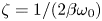 $\zeta =1/(2\beta \omega _0)$ is the damping ratio of the electrical circuit. We obtain a simple expression of the optimal frequency ratio that leads to the maximum energy output
 \begin{equation} \left(\dfrac{\omega_0}{\omega}\right)_{opt}\approx\dfrac{1}{\sqrt{1+2\zeta^2\pm2\zeta\sqrt{1+\zeta^2}}}=\varPi(\zeta). \end{equation}
If plotting (4.5) by adopting the negative sign in figure 10(c), we see all the optimal frequency ratios appearing in the RLC-circuit regime (see figure 10a,b) are located near the prediction (the black solid curve) in the underdamped zone, following a similar trend. Due to the damping effect exerted by the circuit on the flag dynamics, all these values are located above the prediction curve. It is interesting to see that (4.5), if adopting the positive sign, also captures all the optimal frequency ratios appearing in the RC-circuit regime, even though they collapse at the same point in the overdamped zone. Overall speaking, (4.5) provides a fairly good prediction of the optimal frequency for the electrohydroelastic flag where the electrical damping ratio is known.
Although very insightful, (4.5) includes the system response frequency  $\omega$, which is unknown beforehand. To better facilitate the selection of electrical circuit for energy harvesting, especially when the electrical load (
 $\beta$) is known and the inductance (
 $\ell$ or
 $\omega _0$) is to be determined,
 $C_p$ contours for the moderate and less flexible flags are plotted in the
 $\omega _0-\beta$ space, as shown in figure 12(a,b), respectively, in which all the optimal cases (with maximum
 $C_p$ for given
 $\beta$) are marked with red circles. To underline the potential of performance enhancement by using RLC circuits, figure 12(c,d) further compare the maximum
 $C_p$ values at various
 $\beta$ when the RC or RLC circuit is deployed, which are extracted from the contours. Obviously, at lower
 $\beta$ (the range varies with the stiffness of the flag), the maximum
 $C_p$ is achieved with RC circuits, indicating that the employment of an inductor fails to improve the system performance. At higher
 $\beta$, on the contrary, the best performance is achieved by RLC circuits (i.e. with non-zero
 $\omega _0$) through the ‘lock-in’. The boundary that separates these two optimal regimes, as shown in the figure, is the
 $\zeta =1.0$ (the critical damping) line. The implication is that, to trigger the ‘lock-in’ state, one should carefully choose the inductance
 $\omega _0$ to ensure the damping ratio falls into the underdamped zone, i.e.
 $\omega _0>1/2\beta$, which defines the lower bound of the optimal
 $\omega _0$.
(a,b) Contour map of  $C_p$ in the
 $\beta -\omega _0$ space and (c,d) comparison of
 $C_p$ between the optimal RLC circuit (extracted from the contour maps along the red trajectories) and the RC circuit: (a,c) the moderate flexible flag and (b,d) the less flexible flag. Panels show (a)
 $K^*=0.25$, (b)
 $K^*=0.4$, (c)
 $K^*=0.25$, (d)
 $K^*=0.4$.

It is also observed from figure 12 that, in the underdamped zone (i.e.  $\zeta <1$), the maximum
 $C_p$ generally decreases with
 $\beta$ despite some local peak or plateau. This suggests a possible upper bound for the optimal
 $\omega _0$. From (4.5), we can obtain in the underdamped zone the maximum value of optimal
 $\omega _0/\omega$, i.e.
 $\max (\omega _0/\omega )_{opt}\approx 2.4$, which corresponds to the intersection point value of the (4.5) curve and the
 $\zeta =1$ line, as denoted in figure 10(c). Note that, when undergoing the flutter modes, the flapping frequency of the electrohydroelastic flag
 $\omega$ is upper bounded by the frequency of the pure mechanical flag
 $\omega _s$, i.e.
 $\omega <\omega _{s}$, which is evidenced in figure 6(a,c). This leads to a reasonable upper bound for optimal
 $\omega _0$, i.e.
 $\omega _0<2.4\omega _s$. Therefore, the optimal
 $\omega _0$ shall be chosen in a double-bounded range as
 \begin{equation} 0.5\beta^{-1}<\omega_0<2.4\omega_{s}. \end{equation}
This bounded range is depicted by the triangle zone formed with the two black dashed lines shown in figure 12(a,b). Note that some optimal  $\omega _0$ value slightly falls outside this triangle zone, especially near the
 $\zeta =1$ line (see figure 12b). This can be attributed to the general underestimation made by (4.5) through ignoring the damping the circuit brings to the electrohydroelastic flag. Nevertheless, the bounded range described by (4.6) still delineates an acceptable zone for optimal
 $\omega _0$.
Note that (4.6) requires a condition
 \begin{equation} \beta > 0.21\omega_s^{-1}. \end{equation}
It indicates that, if one would like to utilize RLC circuits to achieve better performance over RC circuits, the electrical load  $\beta$ must be greater than a critical value, i.e.
 $0.21\omega _s^{-1}$. Otherwise, the use of RLC circuits cannot bring any benefit.
The optimal frequency ratio (4.5), the proposed searching zone for the optimal  $\omega _0$ (4.6) and the critical electrical load (4.7) are very useful in guiding the optimization process of the electrical circuits. They can assist in choosing an appropriate inductor quickly and efficiently when RLC circuits are needed for higher energy production, which usually happens at relatively large electrical load.
It should be pointed out that, although the free-stream velocity  $U^*$ is not explicitly adopted as a design variable in the above optimization process, its influence has already been reflected in (4.5)–(4.7). Specifically, in (4.5) it affects
 $\omega$, the actual response frequency of the system, through complex fluid–structure–electric coupling, whereas in (4.6) and (4.7) it affects the ranges of
 $\omega _0$ and
 $\beta$ through
 $\omega _s$, the flutter frequency of the pure mechanical flag.
5. Conclusions and discussion
The present study focuses on the multi-physics dynamics of an inverted electrohydroelastic flag. The mechanical energy of ambient flows is harvested through FIV, which is then converted into electricity via an electric circuit. By using a fully coupled fluid–structure–electric model, we simulate the entire energy conversion process, with the focus placed on the dynamics of the flag and its energy output, particularly the impacts of structural and electrical parameters.
Via parametric studies, a variety of structural response modes are identified. Among these response modes, the two flutter modes, i.e. the symmetric- and asymmetric-flutter modes, are the most suitable ones for sustainable energy harvesting. We found that, with moderate flexibility, the flag is more likely to fall into the flutter modes, whereas too flexible flags can be easily bent and deflected to one side considerably (large-deflection mode) and too rigid flags tend to remain almost undeformed (small-deflection mode). We also found that, with only an RC circuit deployed, the increase of electrical load (i.e.  $\beta$) can stabilize the flag.
For benchmark purposes, the energy harvesting performance of the flag equipped with an RC circuit is first examined. Our simulation results and DMD-analysis-based derivations confirm the optimal condition, i.e.  $\beta \omega \sim O(1)$, for the maximum energy output. However, unlike in the weak electromechanical coupling scenario, where this optimal condition works very well, the strong coupling considered in the present study connotes more complicated nonlinear fluid–structure–electric interaction and pushes this condition towards the lower bound of
 $O(1)$.
We then proceed to study the impact of inductors on the performance of the system. By adding an inductor, the output loop becomes an oscillatory RLC circuit with an undamped natural frequency  $\omega _0$. Our results show that, when the circuit's natural frequency
 $\omega _0$ satisfies
 $0.5\beta ^{-1}<\omega _0<2.4\omega _{s}$ (i.e. (4.6)), the employment of the oscillatory circuit tends to lock the structural vibration frequency into the circuit's frequency, which can significantly improve the energy harvesting performance. This performance improvement due to the ‘lock-in’ can only occur in the underdamped zone. Furthermore, the optimal
 $\omega _0$ can be estimated by (4.5). These findings and guidelines are expected to play an important role in the RLC circuit design and optimization.
In the present study, an RLC circuit is used to harvest the energy from ambient flows. However, we note that the simplified electrical rendition is still far from the real system to be developed. For example, for voltage compatibility, electrical interfaces need to be applied between the terminal electric load and the piezoelectric element (Sarker et al. Reference Sarker, Julai, Sabri, Said, Islam and Tahir2019). The most frequently used interface is the combination of a diode rectifier bridge and a filter capacitor, which are respectively used for rectifying and smoothing the alternating voltage (Lefeuvre et al. Reference Lefeuvre, Badel, Richard, Petit and Guyomar2006). Moreover, more complicated interfaces based on the so-called synchronized switching harvesting with inductor technique based on a specific nonlinear processing of the voltage have been proposed (Daniel et al. Reference Daniel, Joachim, Friedrich, Eduardas, Elham and Yiannos2016; Li, Roy & Calhoun Reference Li, Roy and Calhoun2019). Such interfaces can significantly affect the dynamics of the flag and influence the energy output. Therefore, a complete multi-physics model that involves an electric interface may be a better option, whose results can be directly used for guiding the prototype development. This will be our future direction in this area.
Funding
This work was supported by Research Grants Council of Hong Kong under General Research Fund (grant number 15218421); the Hong Kong Polytechnic University Shenzhen Research Institute (grant number J2023A011); and the Hong Kong Polytechnic University under Postdoc Matching Fund Scheme (X.B., grant number W211).
Declaration of interests
The authors report no conflict of interest.
Appendix A. Validation of the numerical model
A.1. Validation of the fluid–structure interaction solver
We verify the accuracy of the fluid–structure interaction solver with two canonical tests. The first one is the relaxation test of a conventional cantilevered filament (whose trailing edge is free and the leading edge is fixed) in an axial flow. The second test is to simulate the flow-induced flutter motion of an inverted cantilevered flag in an incoming flow. Both tests are performed by setting the electromechanical coupling factor  $\alpha$ to zero to remove the influence of the electrical circuit.
For the first test, the initial state of the filament is defined by the equation
 \begin{align} \boldsymbol{X}_{j-1}=\boldsymbol{X}_{j}-\Delta s[\cos((N-j)a),-\sin((N-j)a)], \quad \boldsymbol{V}_j=0, \quad j=N,N-1,\ldots 2, \end{align}
where  $a$ is a small number (here, we choose
 $a=0.01$),
 $N$ is number of Lagrangian nodes along
 $s$. Note that the trailing end of the flag is fixed, i.e.
 $\boldsymbol {X}_1=\boldsymbol {V}_1=0$. Released from the strained configuration described by (A1), the motion of the conventional filament under the effects of the fluid field and gravity is then examined using our fluid–structure interaction model at
 $Re=300, m^{*}=1.0, K^*=0.001, F_r=0.5$ (Froude number). The lateral position of the tip
 $y_{tip}$ is measured throughout the vibration. As displayed in figure 13(a), our simulation perfectly reproduces the time evolution of the tip motion reported in a previous numerical experiment (Huang et al. Reference Huang, Shin and Sung2007). In the second test, induced by the fluid instability the inverted cantilever flag displays self-sustained flutter motion with a certain frequency. As shown in figure 13(b), the present study acquires nearly identical motion amplitude and frequency as existing numerical and experimental works (Kim et al. Reference Kim, Cosse, Cerdeira and Gharib2013; Ryu et al. Reference Ryu, Park, Kim and Sung2015; Huang, Wei & Lu Reference Huang, Wei and Lu2018). Therefore the two tests prove our hydroelastic solver is accurate and robust.
(a) Time histories of vertical displacement of the regular flag's tip:  $Re=300, m^{*}=1.0, K^*=0.001, F_r=0.5$. (b) Time histories of the vertical displacement of the inverted flag:
 $Re=250, m^{*}=1.0, K^*=0.25$.

A.2. Validation of the structure–electrical model
A.2.1. Forced vibration of a piezoelectric flag
The validity of the structure–electric model is firstly assessed with a canonical case, in which a cantilever piezoelectric flag experiences forced vibration in the absence of the ambient flow. Following Shoele & Mittal (Reference Shoele and Mittal2016), the flag vibration is driven by the prescribed periodic heaving motion of the fixed end:  $y_0=A_0\sin (\bar {\omega }t)$, in which
 $A_0$ is a sufficiently small amplitude catering to the small-deflection assumption so that nonlinearities can be neglected. Here, it is chosen to be
 $0.002L$. Assuming the vertical displacement of the flag
 $y(s,t)=Re[Y(s)\textrm {e}^{\textrm {i}\omega t}]$ and the generated voltage
 $\upsilon (s,t)=\textrm {Re}[V(s)\textrm {e}^{\textrm {i}\omega t}]$, we then conduct modal analysis on the piezoelectric equations (3.12), yielding
 \begin{equation} \dfrac{{\rm d}^4Y}{{\rm d}s}-\kappa(\omega)^4Y=0, \end{equation}
in which
 \begin{equation}
\kappa(\omega)= \sqrt[4]{\frac{\omega^2}{m^*K^*}\left[1-\frac{\beta\alpha^2\omega}{\beta(\omega_0^2-\omega^2)+{\rm
i}\omega}\right]^{-1}}.
\end{equation}
By solving the above equation with boundary conditions, the deflection of the free end is formulated as
 \begin{equation} Y_{tip}=\frac{\cos\left(\kappa(\bar{\omega})\right)+\cosh\left(\kappa(\bar{\omega})\right)}{\cos\left(\kappa(\bar{\omega})\right)\cosh\left(\kappa(\bar{\omega})\right)+1}. \end{equation}
Herein, the forced vibration is simulated with our structure–electric model for two different electrical circuits, i.e. RC ( $\omega _0=0$) and RLC (
 $\omega _0=15$). Other electrical and mechanical parameters are fixed at
 $m^*=1.0, K^*=1.0,\alpha =0.3,\beta =1.0$. In figure 14 we compare the simulation results with the theoretical prediction obtained by (A4). It shows that the simulations are able to capture the natural frequencies of the piezoelectric flag. Note that the implementation of the inductor is found to have negligible impacts on the tip deflection, except for the enlarged damping effect that happens when the excitation frequency coincides the circuit's natural frequency (see the trough in the figure at
 $\omega _0=15$). Our structure–electrical model successfully predicts the damping phenomenon.
Spectrum of the amplification factor at the tip of the piezoelectric flag as functions of the actuation frequency  $\bar {\omega }$,
 $m^*=1.0, K^*=1.0,\alpha =0.3,\beta =1.0$.

A.2.2. Free vibration of a simply supported piezoelectric beam
We then proceed to assess the structure–electrical model's accuracy through a relaxation test, the free vibration of a piezoelectric beam with both ends simply supported. Only with this specific boundary condition is it possible to analytically solve the piezoelectric equations with finite Fourier transform. Using the small-deflection assumption, (3.12) is linearized as
 \begin{equation} \left. \begin{gathered} \frac{\partial^2 y}{\partial t^2} =-m^*K^*\frac{\partial^4 y}{\partial s^4}+\alpha m^*\sqrt{K^*}\frac{\partial^2 \upsilon}{\partial s^2},\\ \beta\frac{\partial^2 \upsilon}{\partial t^2} +\frac{\partial \upsilon}{\partial t}+\beta\omega_0^2\upsilon=-\alpha\beta\sqrt{K^*}\frac{\partial^4 y}{\partial t^2\partial s^2} \end{gathered} \right\}, \end{equation}
and the boundary conditions are  $y=0, \partial ^2 y/\partial s^2=\alpha \upsilon /\sqrt {K^*}$ at
 $s=0$ or
 $s=1$. Solutions of the above linear system can be written as
 \begin{equation} y(s,t)=2\sum_{n=1}^{\infty}\hat{y}(n,t)\sin(n{\rm \pi} s), \quad \upsilon(s,t)=2\sum_{n=1}^{\infty}\hat{\upsilon}(n,t)\sin(n{\rm \pi} s), \end{equation}
in which the coefficients are given by
 \begin{equation} \hat{y}(n,t)=\int_0^1y(s,t)\sin(n{\rm \pi} s)\,{\rm d}s, \quad \hat{\upsilon}(n,t)=\int_0^1\upsilon(s,t)\sin(n{\rm \pi} s)\,{\rm d}s. \end{equation}
We multiply (A5) by  $\sin (n{\rm \pi} s)$ and integrate with respect to
 $s$ from 0 to 1, yielding
 \begin{equation} \left. \begin{gathered} \frac{\partial^2 \hat{y}}{\partial t^2} +m^*K^*n^4{\rm \pi}^4\hat{y}=-\alpha m^*\sqrt{K^*}n^2{\rm \pi}^2\hat{\upsilon},\\ \beta\frac{\partial^2 \hat{\upsilon}}{\partial t^2} +\frac{\partial\hat{\upsilon}}{\partial t}+\beta\omega_0^2\hat{\upsilon}=\alpha\beta\sqrt{K^*} n^2{\rm \pi}^2\frac{\partial^2 \hat{y}}{\partial t^2}. \end{gathered} \right\} \end{equation}
We take the solutions of the eigenvalue problem as  $\hat {y}=\hat {Y}\textrm {e}^{\textrm {i}\omega _nt}$ and
 $\hat {\upsilon }=\hat {\varUpsilon }\textrm {e}^{\textrm {i}\omega _nt}$ and substitute into (A8), yielding
 \begin{equation} \left. \begin{gathered} (-\omega_n^2+m^*K^*n^4{\rm \pi}^4)\hat{Y} +\alpha m^*\sqrt{K^*}n^2{\rm \pi}^2\hat{\varUpsilon}=0,\\ (-\beta\omega_n^2+{\rm i}\omega_n+\beta\omega_0^2)\hat{\varUpsilon} +\alpha\beta\sqrt{K^*} n^2{\rm \pi}^2\omega_n^2\hat{Y}=0. \end{gathered} \right\} \end{equation}
The equation can be further reduced to the characteristic equation of the eigenvalue problem
 \begin{align} &\beta\omega_n^4-{\rm
i}\omega_n^3-\beta\left(
m^*K^*n^4{\rm \pi}^4(1+\alpha^2)+\omega_0^2\right)\omega_n^2+{\rm i}
m^*K^*n^4{\rm \pi}^4\omega_n\notag\\ &\quad +\beta\omega_0^2m^*K^*n^4{\rm \pi}^4=0.
\end{align}
Each solution  $\omega _{n,j}$ (
 $\,j=1,2,3,4$) of the fourth-order polynomial equation corresponds to a normal mode vector
 \begin{equation} \left(\begin{array}{@{}c@{}}{\hat{Y}^{(\,j)}}\\ {\hat{\varUpsilon}^{(\,j)}}\end{array}\right){\rm e}^{{\rm i}\omega_{n,j}t} =\left(\begin{array}{@{}c@{}}{\hat{Y}^{(\,j)}}\\ {r^{(\,j)}\hat{Y}^{(\,j)}}\end{array}\right){\rm e}^{{\rm i}\omega_{n,j}t}, \end{equation}
in which  $r^{(\,j)}$ is obtained by substituting
 ${\omega _{n}}_j$ into (A9), leading to
 \begin{equation} r^{(\,j)}=\frac{\omega_{n,j}^2-m^*K^*n^4{\rm \pi}^4}{\alpha\sqrt{K^*}m^*n^2{\rm \pi}^2}. \end{equation}
Thus, the general solution to (A8) is calculated by the linear superposition of the four normal modes  $\hat {y}(n,t)=\sum _{j=1}^4\hat {Y}^{(\,j)}\textrm {e}^{\textrm {i}\omega _{n,j}t}$ and
 $\hat {\upsilon }(n,t)=\sum _{j=1}^4r^{(\,j)}\hat {Y}^{(\,j)}\textrm {e}^{\textrm {i}\omega _{n,j}t}$, where the four unknowns
 $\hat {Y}^{(\,j)}$ can be determined from initial conditions:
 $y(s,t=0)=y_0(s)$,
 $\upsilon (s,t=0)=\upsilon _0(s)$,
 ${\textrm {d} y}/\textrm {d}t(s,t=0)=\dot {y}_0(s)$ and
 $\textrm {d}\upsilon /\textrm {d}t(s,t=0)=\dot {\upsilon }_0(s)$. The finite Fourier sine transforms of the initial conditions yield
 \begin{equation} \left. \begin{gathered} \hat{y}(n,t=0)=\int_0^1y_0(s)\sin(n{\rm \pi} s)\,{\rm d}s, \\ \frac{{\rm d}\hat{y}}{{\rm d}t}(n,t=0)=\int_0^1\dot{y}_0(s)\sin(n{\rm \pi} s)\,{\rm d}s,\\ \hat{\upsilon}(n,t=0)=\int_0^1\upsilon_0(s)\sin(n{\rm \pi} s)\,{\rm d}s ,\\ \frac{{\rm d}\hat{\upsilon}}{{\rm d}t}(n,t=0)=\int_0^1\dot{\upsilon}_0(s)\sin(n{\rm \pi} s)\,{\rm d}s. \end{gathered} \right\} \end{equation}
Finally, the solutions of (A5) can be calculated by substituting  $\hat {y}(n,t)$ and
 $\hat {\upsilon }(n,t)$ into (A6a,b).
Here, we set  $y_0(s)=a\sin ({\rm \pi} s)$ (
 $a=0.001$) and
 $\dot {y}_0=\upsilon _0=\dot {\upsilon }_0=0$, such that all modes except for the first one disappear due to the orthogonality of trigonometric functions. The solutions turn out to be
 $y(s,t)=2\sum _{j=1}^{4}\hat {Y}^{(\,j)}\textrm {e}^{\textrm {i}\omega _{1,j}t}\sin ({\rm \pi} s)$ and
 $\upsilon (s,t)=2\sum _{j=1}^{4}r^{(\,j)}\hat {Y}^{(\,j)}\textrm {e}^{\textrm {i}\omega _{1,j}t}\sin ({\rm \pi} s)$. In figure 15 we compare our numerical predictions of
 $y(0.5,t)$ and
 $\upsilon (0.5,t)$ (measured at the beam centroid) with the analytical solutions for the case of
 $\alpha =0.3,\omega _0=10,\beta =K^*=m^*=1.0$. As is shown in the figure, the numerical results are in good agreement with the theoretical analysis, verifying the validity of our piezoelectric model.
Time histories of the (a) deflection and (b) electric voltage at the centroid of the beam ( $s=0.5$),
 $\alpha =0.3,\omega _0=10,\beta =K^*=m^*=1.0$.

A.3. Validation of the entire piezohydroelastic model
Having verified the robustness of the two ‘submodules’ (i.e. the fluid–structure and structure–electrical interactions), we then focus on the whole fluid–structure–electrical model in this section. The energy harvesting capability of the piezohydroelastic system with purely resistive circuit is evaluated at various electroelastic coupling coefficients  $\alpha$ and tuning coefficients
 $\beta$. As shown in figure 16, the efficiencies predicted by our model are in perfect accord with the simulation data from the reference (Shoele & Mittal Reference Shoele and Mittal2016), proving that the piezohydroelastic model is reliable and accurate.
Energy harvesting efficiency  $C_p$ as functions of the product of the structural frequency
 $\omega$ and the tuning coefficient
 $\beta$ when
 $\omega _0=0,K^*=0.25,m^*=1.$

Appendix B. Dynamic mode decomposition of the mechanoelectrical system
Dynamic mode decomposition (Kutz et al. Reference Kutz, Brunton, Brunton and Proctor2016) is a data decomposition method that serves to extract a coherent relevant data structure and its temporal dynamics (e.g. growth rate and frequency) from a sequence of discrete data. In our case the variable of interest is the local curvature  $\mathscr {\varLambda }$, thus a time series of
 $\mathscr {\varLambda }$ with equal time interval
 $\Delta T$ is synthesized into a matrix as
 \begin{equation} \mathscr{\varLambda}_1^m=\begin{bmatrix} | & | & & |\\ \mathscr{\varLambda}_1 & \mathscr{\varLambda}_2 & \cdots & \mathscr{\varLambda}_m\\ | & | & & | \end{bmatrix}, \end{equation}
where  $m$ is the number of time snapshots and each column represents the discrete distribution of
 $\mathscr {\varLambda }$ along the flag for each snapshot, e.g.
 \begin{equation} \mathscr{\varLambda}_1=\begin{bmatrix} \mathscr{\varLambda}_1({\Delta s})\\ \mathscr{\varLambda}_1({2\Delta s})\\ :\\ \mathscr{\varLambda}_1({N\Delta s}) \end{bmatrix}, \end{equation}
in which  $\Delta s$ is the spatial interval corresponding to the Lagrangian grid size, and
 $N$ is the size of the vector. Even though those snapshots are normally obtained from a nonlinear process, DMD aims to find an optimal linear operator
 $\mathscr {A}$ to achieve inter-snapshot linear mapping between any two consecutive snapshots, i.e.
 $\mathscr {\varLambda }_{i+1}=\mathscr {A}\mathscr {\varLambda }_i$. Physically, this process can be interpreted as the linear–tangent approximation of a nonlinear dynamic. Given the constant mapping between the snapshots, the operator
 $\mathscr {A}$ becomes a linear mapping from data sequence
 $\mathscr {\varLambda }_1^{m-1}$ to
 $\mathscr {\varLambda }_2^{m}$:
 \begin{gather} \mathscr{\varLambda}_2^m=\begin{Bmatrix} \mathscr{\varLambda}_2 , \mathscr{\varLambda}_3 ,\ldots,\mathscr{\varLambda}_m \end{Bmatrix} =\mathscr{A}\begin{Bmatrix} \mathscr{\varLambda}_1 , \mathscr{\varLambda}_2 ,\ldots,\mathscr{\varLambda}_{m-1} \end{Bmatrix}=\mathscr{A}\mathscr{\varLambda}_1^{m-1} \end{gather}
 \begin{gather} \mathscr{A}=\mathscr{\varLambda}_2^m \boldsymbol{\cdot}(\mathscr{\varLambda}_1^{m-1})^{\dagger} . \end{gather}
The DMD computes the leading eigendecomposition of  $\mathscr {A}$ to obtain the dynamic modes (
 $\phi$) and their corresponding eigenvalues (
 $\lambda$).
With eigenvalues and eigenvectors of  $\mathscr {A}$ determined, the curvature distribution of arbitrary snapshot at time
 $t_k=k\Delta T$ can be reconstructed by
 \begin{equation} \mathscr{\varLambda}(t_k)=\sum_{j=0}^{m}b_j\lambda_j^{k-1}\phi_j, \end{equation}
where  $b_j$ denotes the magnitude of the discrete mode
 $\phi _j$.
 $\lambda$,
 $\phi$ and
 $b_j$ are all complex quantities. Since the sampled curvature is real, the complex eigenvalues and eigenmodes will be conjugated, thus the imaginary part will disappear in doing above summation.
A continuous projected solution may be derived from the above discrete expression. By assuming  $\omega _j=\ln (\lambda _j)/\Delta T$, continuous time evolution of the problem is then given by
 \begin{equation} \mathscr{\varLambda}(t)=\sum_{j=0}^{m}b_j {\rm e}^{\omega_jt} \phi_j. \end{equation}
The real part of  $\omega _j$ represents exponential growth or decay rate, and the imaginary part contains the temporal frequency. Due to the periodicity of the structural deformation the growth rate should be negligible, i.e.
 $\textrm {Re}\{\omega _j\}\approx 0$. Plugging (B6) into the electrical governing equation (3.12) yields
 \begin{equation} \frac{\partial^2 \upsilon}{\partial t^2}+\frac{1}{\beta}\frac{\partial \upsilon}{\partial t}+\omega_0^2\upsilon=-\alpha\sqrt{K^*}\sum_{j}b_j{{\rm Im}\{\omega_j\}}^2{\rm e}^{{\rm Im}\{\omega_j\}{\rm i} t} \phi_j. \end{equation}
In damped systems, the oscillation in the natural frequency is usually damped out rapidly and only the steady state solution is left. The voltage output of one arbitrary mode  $\phi _j$ at
 $s_{\imath }=\imath \Delta s$ is
 \begin{equation} \upsilon_j(s_{\imath},t)=\dfrac{-\alpha\sqrt{K^*} b_j{\rm Im}\{\omega_j\}^2\phi_j(s_{\imath})}{\omega_0^2-{\rm Im}\{\omega_j\}^2+\dfrac{{\rm Im}\{\omega_j\}}{\beta} {\rm i}} {\rm e}^{{\rm Im}\{\omega_j\}{\rm i} t}, \end{equation}
whose imaginary component can be zeroed out by summing its conjugate counterpart. The real part can be expressed by
 \begin{equation} {\rm Re}\left\{\upsilon_j(s_{\imath},t)\right\}=-2\hat{\upsilon}_j|\phi_j(s_{\imath})|\cos\left({\rm Im}\{\omega_j\}t+\theta_1+\theta_2(s_{\imath})-\theta_3\right), \end{equation}
where
 \begin{equation} \hat{\upsilon}_j=\dfrac{\alpha\sqrt{K^*} {\rm Im}\{\omega_j\}^2}{\sqrt{\left({\rm Im}\{\omega_j\}^2-\omega_0^2\right)^2+\dfrac{{\rm Im}\{\omega_j\}^2}{\beta^2}}}|b_j|, \end{equation}
where the operator  $| {\cdot } |$ calculates the magnitude of the complex number,
 $\theta _1$,
 $\theta _2(s_{\imath })$ and
 $\theta _3$ represent the argument of
 $b_j$,
 $\phi _j(s_{\imath })$ and
 $\omega _0^2-\textrm {Im}\{\omega _j\}^2+({\textrm {Im}\{\omega _j\}}/{\beta })\textrm {i}$, respectively. Thus the energy output sourced from a pair of conjugate modes is
 \begin{equation} C_{p,j}\approx\dfrac{4\hat{\upsilon}_j^2}{\beta}\sum_{\imath=1}^N\left[|\phi_j(s_{\imath})|^2\int_T \cos^2[{\rm Im}\{\omega_j\}t+\theta_1+\theta_2(s_{\imath})-\theta_3]\,{\rm d}t/T\right]\Delta s=\frac{2\hat{\upsilon}_j^2\Delta s}{\beta}, \end{equation}
in which  $T=2{\rm \pi} /\textrm {Im}\{\omega _j\}$. Note that the modulus of each mode equals to unity, i.e.
 \begin{equation} \sum_{\imath=1}^N|\phi_j(s_\imath)|^2=1, \quad s_\imath=\imath\Delta s. \end{equation}
Assuming that the spatial equation  $\varPhi _j(s)$ is the continuous mode corresponding to
 $\phi _j(s_\imath )$, one can obtain
 \begin{equation} \int_0^1|\varPhi_j(s)|^2\,{\rm d}s\approx\sum_{\imath=1}^N|b_j|^2|\phi_j(s_\imath)|^2\Delta s=|b_j|^2\Delta s=|b_j|^2/N. \end{equation}
Since the left-hand side of the above equation is a constant for a given case,  $|b_j|^2$ should be proportional to
 $1/\Delta s$ (i.e.
 $N$). As a result,
 $C_{p,j}$ is proven to be independent to the sampling interval
 $\Delta s$ (or
 $N$) after a close inspection of (B10) and (B11). To avoid confusion, in the following
 $|b_j|^2/N$ will be only presented as a normalized term
 $|b_j|^2$.
Within a certain DMD framework,  $C_p^j$ scales with
 $\hat {\upsilon }_j^2/\beta$, which is calculated by
 \begin{equation} \dfrac{\hat{\upsilon}_j^2}{\beta}=\dfrac{\alpha^2K^*{\rm Im}\{\omega_j\}^4}{\beta\left({\rm Im}\{\omega_j\}^2-\omega_0^2\right)^2+\dfrac{{\rm Im}\{\omega_j\}^2}{\beta}}|b_j|^2. \end{equation}
Specifically, when the inductive element is absent ( $\omega _0=0$), we have
 \begin{equation} \dfrac{\hat{\upsilon}_j^2}{\beta}=\dfrac{\alpha^2K^*|b_j|^2}{\beta+\dfrac{1}{\beta {\rm Im}\{\omega_j\}^2}}. \end{equation}


 Open access

