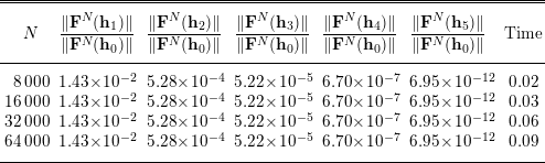
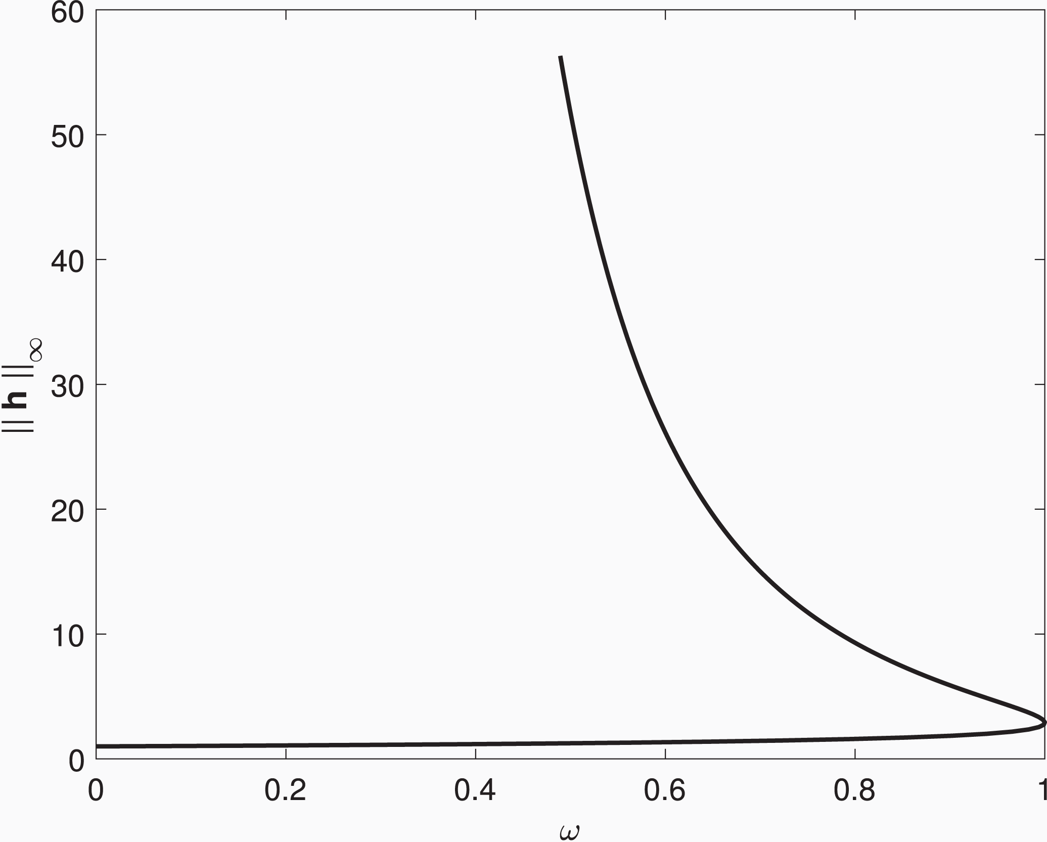
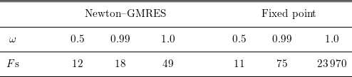
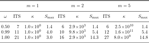
1 Introduction
Nonlinear equations are ubiquitous, and methods for their solution date from the quadratic formula. Modern numerical methods are, for the most part, based on Newton’s method or Picard iteration.
Most of the results in this paper, while stated and proved in a finite-dimensional setting, do not depend on compactness of the unit ball and are valid in a Banach space setting (see Section 2.9). We will explicitly point out the few exceptions.
This subject is old (Newton Reference Newton1967–1976, Raphson Reference Raphson1690, Picard Reference Picard1890). Ortega and Rheinboldt (Reference Ortega and Rheinboldt1970), Dennis and Schnabel (Reference Dennis and Schnabel1996) and Kelley (Reference Kelley1995) are our primary sources for notation and analysis of the classical methods. The bibliographies of these books vividly illustrate the rich classical literature in this field. The approach we take in this article is not the only one. Deuflhard (Reference Deuflhard2004), for example, has a somewhat different viewpoint.
We intend this article to be self-contained for any student of numerical analysis. To that end we summarize the classical theory of Newton and Newton-iterative methods in Section 2. The remaining sections have less familiar material and could in many ways be thought of as a second volume of Kelley (Reference Kelley1995). The topics in Sections 5 and 6, in particular, are very active areas of research.
1.1 Notation
We seek to solve nonlinear equations in
 $\mathbb{R}^{N}$
. We will write vectors in boldface lower-case, maps on vectors in boldface upper-case, and components of vectors as lower-case roman letters. For example, if
 $\mathbf{x}\in \mathbb{R}^{N}$
,
 $x_{i}$
is the
 $i$
th component of
 $\mathbf{x}$
. The methods are iterative, and we will denote the sequence of iterations by
 $\{\mathbf{x}_{n}\}$
when the entire sequence (or several elements of the sequence) is of interest. In many cases only the current iteration
 $\mathbf{x}_{c}$
and the next one
 $\mathbf{x}_{+}$
are needed, and we can express the algorithm in terms of the transition from
 $\mathbf{x}_{c}$
to
 $\mathbf{x}_{+}$
.
Two formulations of nonlinear equations are of interest in this article.
1.2 Root finding formulation and Newton’s method
The ‘root finding’ form is
 $$\begin{eqnarray}\mathbf{F}(\mathbf{x})=0,\end{eqnarray}$$
where
 $\mathbf{F}:\mathbb{R}^{N}\rightarrow \mathbb{R}^{N}$
,
 $$\begin{eqnarray}\mathbf{F}(\mathbf{x})=\left(\begin{array}{@{}c@{}}f_{1}(\mathbf{x})\\ f_{2}(\mathbf{x})\\ \vdots \\ f_{N}(\mathbf{x})\end{array}\right)\!.\end{eqnarray}$$
We will refer to
 $\mathbf{F}$
as the residual.
If
 $\mathbf{F}$
is differentiable at
 $\mathbf{x}$
, we will denote the Jacobian matrix by
 $\mathbf{F}^{\prime }(\mathbf{x})$
. Recall that
 $$\begin{eqnarray}\mathbf{F}^{\prime }(x)_{ij}=\unicode[STIX]{x2202}f_{i}(x)/\unicode[STIX]{x2202}x_{j}.\end{eqnarray}$$
When we express an equation in this form we will be solving it with a variation of Newton’s method. The classical version of Newton’s method takes
 $\mathbf{x}_{c}$
to
 $\mathbf{x}_{+}$
via
 $$\begin{eqnarray}\mathbf{x}_{+}=\mathbf{x}_{c}-\mathbf{F}^{\prime }(\mathbf{x}_{c})^{-1}\mathbf{F}(\mathbf{x}_{c}).\end{eqnarray}$$
Implicit in (1.2) is the solution of the linearized equation for the step
 $\mathbf{s}$
:
 $$\begin{eqnarray}\mathbf{F}^{\prime }(\mathbf{x}_{c})\mathbf{s}=-\mathbf{F}(\mathbf{x}_{c}).\end{eqnarray}$$
The various formulations of Newton’s method we consider in Section 2 differ in the way they approximate a solution to (1.3). In Section 6 we show how to relax the smoothness assumptions on
 $\mathbf{F}$
.
1.3 Fixed-point formulation and Picard iteration
The fixed-point formulation of a nonlinear equation is
 $$\begin{eqnarray}\mathbf{x}=\mathbf{G}(\mathbf{x}),\end{eqnarray}$$
where
 $\mathbf{G}:\mathbb{R}^{N}\rightarrow \mathbb{R}^{N}$
. The two formulations are equivalent via
 $\mathbf{F}(\mathbf{x})=\mathbf{x}-\mathbf{G}(\mathbf{x})$
, of course, but the choice of formulation usually carries meaning. In particular, the use of the fixed-point formulation will imply, at least in this article, that derivative information is either not necessary or difficult to obtain when designing the algorithms. Picard iteration (Picard Reference Picard1890),
 $$\begin{eqnarray}\mathbf{x}_{+}=\mathbf{G}(\mathbf{x}_{c}),\end{eqnarray}$$
is the classic example of a method that does not use Jacobian information. Picard iteration is also called fixed-point iteration, Richardson iteration or successive substitution. Ortega and Rheinboldt (Reference Ortega and Rheinboldt1970) make a distinction between some of these terms, but we see no reason for that, and our usage reflects common practice. Tapia, Dennis and Schäfermeyer (Reference Tapia, Dennis and Schäfermeyer2018) have an interesting historical perspective.
We will solve fixed-point problems with Picard iteration or one of its variations.
We close this section with the well-known theory for Picard iteration.
Definition 1.1. A map
 $\mathbf{G}$
is a contraction on a closed set
 ${\mathcal{D}}\subset \mathbb{R}^{N}$
if
∙
 $\mathbf{G}(\mathbf{x})\in {\mathcal{D}}$
if
$\mathbf{x}\in {\mathcal{D}}$
,
∙ there is
$\unicode[STIX]{x1D6FC}\in (0,1)$
such that for all$$\begin{eqnarray}\Vert \mathbf{G}(\mathbf{x})-\mathbf{G}(\mathbf{y})\Vert \leq \unicode[STIX]{x1D6FC}\Vert \mathbf{x}-\mathbf{y}\Vert ,\end{eqnarray}$$
$\mathbf{x},\mathbf{y}\in {\mathcal{D}}$
.


The convergence result is the contraction mapping theorem.
Theorem 1.2. If
 $\mathbf{G}$
is a contraction on a closed set
 ${\mathcal{D}}\subset \mathbb{R}^{N}$
, then
∙ there is a unique solution
$\mathbf{x}^{\ast }\in {\mathcal{D}}$
to
$\mathbf{x}=\mathbf{G}(\mathbf{x})$
,∙ if
$\mathbf{x}_{0}\in {\mathcal{D}}$
then the Picard iteration converges to
$\mathbf{x}^{\ast }$
.


We refer to Ortega and Rheinboldt (Reference Ortega and Rheinboldt1970) and Kelley (Reference Kelley1995) for the familiar proof. We will discuss an important extension of Picard iteration in Section 5.
2 Newton’s method: classical algorithms
For most of this section we will make the so-called standard assumptions on the nonlinear equation
 $\mathbf{F}(\mathbf{x})=0$
.
Assumption 2.1. There are
 $\mathbf{x}^{\ast }\in \mathbb{R}^{N}$
and
 $\unicode[STIX]{x1D70C}^{\ast }>0$
such that
∙
$\mathbf{F}(\mathbf{x}^{\ast })=0$
,∙
$\mathbf{F}^{\prime }(\mathbf{x}^{\ast })$
is non-singular, and∙
$\mathbf{F}^{\prime }(\mathbf{x})$
is Lipschitz continuous with Lipschitz constant
$\unicode[STIX]{x1D6FE}$
, that is, (2.1)for all$$\begin{eqnarray}\Vert \mathbf{F}^{\prime }(\mathbf{x})-\mathbf{F}^{\prime }(\mathbf{y})\Vert \leq \unicode[STIX]{x1D6FE}\Vert \mathbf{x}-\mathbf{y}\Vert ,\end{eqnarray}$$
$$\begin{eqnarray}\mathbf{x},\mathbf{y}\in {\mathcal{B}}(\mathbf{x}^{\ast },\unicode[STIX]{x1D70C}^{\ast })\equiv \{\mathbf{z}\mid \Vert \mathbf{z}-\mathbf{x}^{\ast }\Vert \leq \unicode[STIX]{x1D70C}^{\ast }\}.\end{eqnarray}$$


The standard assumptions distinguish the root
 $\mathbf{x}^{\ast }$
of
 $\mathbf{F}$
from any others and the local convergence theory refers only to that root. When non-uniqueness is an issue (see Sections 4 and 7), then the standard assumptions only play a role after a particular root has been identified.
In this section we will analyse the convergence of Newton’s method twice: once for the simple formulation and again to account for errors in the evaluation of
 $\mathbf{F}$
and in the solution of the linearized problem for the step. The latter of the two results, Theorem 2.3, serves to explain not only many classical variations of Newton’s method but also the modern Jacobian-free Newton–Krylov (JFNK) methods (Knoll and Keyes Reference Knoll and Keyes2004) that are the basis of large-scale nonlinear solvers such as KINSOL (Collier, Hindmarsh, Serban and Woodward Reference Collier, Hindmarsh, Serban and Woodward2015), NOX (Heroux et al.
Reference Heroux, Bartlett, Howle, Hoekstra, Hu, Kolda, Lehoucq, Long, Pawlowski, Phipps, Salinger, Thornquist, Tuminaro, Willenbring, Williams and Stanley2005) and SNES (Balay et al.
Reference Balay, Abhyankar, Adams, Brown, Brune, Buschelman, Dalcin, Eijkhout, Gropp, Kaushik, Knepley, McInnes, Rupp, Smith, Zampini and Zhang2015).
2.1 Local convergence of Newton’s method
The reader may know Theorem 2.2 well. The simple statement is that if the standard assumptions hold and the initial iterateFootnote
1
is sufficiently near
 $\mathbf{x}^{\ast }$
(hence the term local), then the Newton iteration
 $\{\mathbf{x}_{n}\}$
exists (i.e.
 $\mathbf{F}^{\prime }(\mathbf{x}_{n})$
is non-singular for all
 $n\geq 0$
) and converges quadratically to
 $\mathbf{x}^{\ast }$
. The Newton iterates are, of course,
 $$\begin{eqnarray}\mathbf{x}_{n+1}=\mathbf{x}_{n}-\mathbf{F}(\mathbf{x}_{n})^{-1}\mathbf{F}(\mathbf{x}_{n}),\end{eqnarray}$$
for
 $n\geq 0$
. This is exactly (1.2) with
 $\mathbf{x}_{c}$
replaced by
 $\mathbf{x}_{n}$
and
 $\mathbf{x}_{+}$
by
 $\mathbf{x}_{n+1}$
. The advantage of the
 $\mathbf{x}_{c}$
and
 $\mathbf{x}_{+}$
notation is that the transition from
 $\mathbf{x}_{c}$
to
 $\mathbf{x}_{+}$
is central and the iteration counter is generally irrelevant to the convergence analysis. Quadratic convergence means that
 $$\begin{eqnarray}\Vert \mathbf{e}_{+}\Vert =O(\Vert \mathbf{e}_{c}\Vert ^{2}),\end{eqnarray}$$
where the error in
 $\mathbf{x}$
is
 $\mathbf{e}=\mathbf{x}-\mathbf{x}^{\ast }$
. Quadratic convergence says that the number of significant figures in the result roughly doubles with each iteration.
We will begin with a precise statement of this result which will, among other things, exhibit the constant in the
 $O$
-term. We will also begin to develop a taxonomy of convergence types. We say that
 $\mathbf{x}_{n}\rightarrow \mathbf{x}^{\ast }$
q-quadratically if (2.2) holds and r-quadratically if there is a real sequence
 $\{\unicode[STIX]{x1D709}_{n}\}$
which converges q-quadratically to
 $0$
such that
 $\Vert \mathbf{e}_{n}\Vert \leq \unicode[STIX]{x1D709}_{n}$
. We say the convergence is q-linear if there is
 $\unicode[STIX]{x1D6FC}\in [0,1)$
such that
 $\Vert \mathbf{e}_{n+1}\Vert \leq \unicode[STIX]{x1D6FC}\Vert \mathbf{e}_{n}\Vert$
for
 $n$
sufficiently large;
 $\unicode[STIX]{x1D6FC}$
is called the q-factor. The convergence is q-superlinear if
 $$\begin{eqnarray}\lim _{n\rightarrow \infty }\displaystyle \frac{\Vert \mathbf{e}_{n+1}\Vert }{\Vert \mathbf{e}_{n}\Vert }=0.\end{eqnarray}$$
Finally, we will quantify ‘sufficiently near
 $\mathbf{x}^{\ast }$
’. At a minimum, all the local convergence results in this section require
 $$\begin{eqnarray}|\mathbf{x}-\mathbf{x}^{\ast }\Vert \leq \min \biggl(\displaystyle \frac{\Vert \mathbf{F}^{\prime }(\mathbf{x}^{\ast })^{-1}\Vert ^{-1}}{2\unicode[STIX]{x1D6FE}},\unicode[STIX]{x1D70C}^{\ast }\biggr),\end{eqnarray}$$
where
 $\unicode[STIX]{x1D6FE}$
is the Lipschitz constant for
 $\mathbf{F}^{\prime }$
and
 $\unicode[STIX]{x1D70C}^{\ast }$
is the radius of the ball about
 $\mathbf{x}^{\ast }$
in which the Lipschitz continuity assumption on
 $\mathbf{F}^{\prime }$
holds.
2.2 Classical Newton’s method
We will prove Theorem 2.2 in detail. Not only is the proof illuminating in its own right, but some of the details lead to algorithmic insights.
Theorem 2.2. Let Assumption 2.1 hold and assume that
 $\mathbf{x}_{c}$
satisfies (2.3). Then
 $\mathbf{F}(\mathbf{x}_{c})$
is non-singular,
 $$\begin{eqnarray}\Vert \mathbf{F}^{\prime }(\mathbf{x}_{c})\Vert ^{-1}\leq 2\Vert \mathbf{F}^{\prime }(\mathbf{x}^{\ast })\Vert ^{-1},\end{eqnarray}$$
and
 $$\begin{eqnarray}\Vert \mathbf{e}_{+}\Vert \leq \Vert \mathbf{F}^{\prime }(\mathbf{x}^{\ast })^{-1}\Vert \unicode[STIX]{x1D6FE}\,\Vert \mathbf{e}_{c}\Vert ^{2}\leq \Vert \mathbf{e}_{c}\Vert /2.\end{eqnarray}$$
Proof. The standard assumptions and (2.3) imply that
 $$\begin{eqnarray}\Vert \mathbf{F}^{\prime }(\mathbf{x}_{c})-\mathbf{F}^{\prime }(\mathbf{x}^{\ast })\Vert \leq \unicode[STIX]{x1D6FE}\Vert \mathbf{e}_{c}\Vert \leq \displaystyle \frac{\Vert \mathbf{F}^{\prime }(\mathbf{x}^{\ast })^{-1}\Vert }{2},\end{eqnarray}$$
and hence
 $$\begin{eqnarray}\Vert \mathbf{I}-\mathbf{F}^{\prime }(\mathbf{x}^{\ast })^{-1}\mathbf{F}^{\prime }(\mathbf{x}_{c})\Vert \leq \Vert \mathbf{F}^{\prime }(\mathbf{x}^{\ast })^{-1}\Vert \Vert \mathbf{F}^{\prime }(\mathbf{x}_{c})-\mathbf{F}^{\prime }(\mathbf{x}^{\ast })\Vert \leq 1/2,\end{eqnarray}$$
so
 $\mathbf{F}^{\prime }(\mathbf{x}^{\ast })^{-1}$
is an approximate inverse of
 $\mathbf{F}^{\prime }(\mathbf{x}_{c})$
, and
 $$\begin{eqnarray}\Vert \mathbf{F}^{\prime }(\mathbf{x}_{c})^{-1}\Vert \leq \displaystyle \frac{\Vert \mathbf{F}^{\prime }(\mathbf{x}^{\ast })^{-1}\Vert }{2},\end{eqnarray}$$
as asserted.
The remainder of the proof follows from the fundamental theorem of calculus, which implies that
 $$\begin{eqnarray}\displaystyle \mathbf{F}(\mathbf{x}_{c}) & = & \displaystyle \int _{0}^{1}\mathbf{F}^{\prime }(\mathbf{x}^{\ast }+t\mathbf{e}_{c})\mathbf{e}_{c}\,\text{d}t\nonumber\\ \displaystyle & = & \displaystyle \mathbf{F}^{\prime }(\mathbf{x}_{c})\mathbf{e}_{c}+\int _{0}^{1}(\mathbf{F}^{\prime }(\mathbf{x}^{\ast }+t\mathbf{e}_{c})-\mathbf{F}^{\prime }(\mathbf{x}_{c}))\mathbf{e}_{c}\,\text{d}t.\end{eqnarray}$$
Hence,
 $$\begin{eqnarray}\displaystyle \mathbf{e}_{+} & = & \displaystyle \mathbf{e}_{c}-\mathbf{F}^{\prime }(\mathbf{x}_{c})^{-1}\biggl(\mathbf{F}^{\prime }(\mathbf{x}_{c})\mathbf{e}_{c}+\int _{0}^{1}(\mathbf{F}^{\prime }(\mathbf{x}^{\ast }+t\mathbf{e}_{c})-\mathbf{F}^{\prime }(\mathbf{x}_{c}))\mathbf{e}_{c}\,\text{d}t\biggr)\nonumber\\ \displaystyle & = & \displaystyle -\mathbf{F}^{\prime }(\mathbf{x}_{c})^{-1}\biggl(\int _{0}^{1}(\mathbf{F}^{\prime }(\mathbf{x}^{\ast }+t\mathbf{e}_{c})-\mathbf{F}^{\prime }(\mathbf{x}_{c}))\mathbf{e}_{c}\,\text{d}t\biggr).\nonumber\end{eqnarray}$$
Note that
 $$\begin{eqnarray}\biggl\|\int _{0}^{1}(\mathbf{F}^{\prime }(\mathbf{x}^{\ast }+t\mathbf{e}_{c})-\mathbf{F}^{\prime }(\mathbf{x}_{c}))\mathbf{e}_{c}\,\text{d}t\biggr\|\leq \int _{0}^{1}\unicode[STIX]{x1D6FE}\Vert \mathbf{e}_{c}\Vert ^{2}(1-t)\,\text{d}t=\unicode[STIX]{x1D6FE}\Vert \mathbf{e}_{c}\Vert ^{2}/2.\end{eqnarray}$$
Hence,
 $$\begin{eqnarray}\displaystyle \Vert \mathbf{e}_{+}\Vert & \leq & \displaystyle \displaystyle \frac{\Vert \mathbf{F}^{\prime }(\mathbf{x}_{c})^{-1}\Vert \unicode[STIX]{x1D6FE}}{2}\Vert \mathbf{e}_{c}\Vert ^{2}\leq \displaystyle \frac{2\Vert \mathbf{F}^{\prime }(\mathbf{x}^{\ast })^{-1}\Vert \unicode[STIX]{x1D6FE}}{2}\Vert \mathbf{e}_{c}\Vert ^{2}\nonumber\\ \displaystyle & \leq & \displaystyle \Vert \mathbf{e}_{c}\Vert /2.\end{eqnarray}$$
This completes the proof and shows that the constant in the
 $O$
-term for quadratic convergence is no larger than
 $\Vert \mathbf{F}^{\prime }(\mathbf{x}^{\ast })^{-1}\Vert \unicode[STIX]{x1D6FE}$
.☐
Our bounds for the distance of the initial iterate from the root and for the convergence rate depend only on the norm of the inverse of the Jacobian at the root and the Lipschitz constant of the Jacobian near the root. This observation leads directly to the Kantorovich theorem (Kantorovich and Akilov Reference Kantorovich and Akilov1982: see Section 3) and the implicit function theorem (Keller Reference Keller1987) in Section 4, which are the basis for the pseudo-arclength continuation method we discuss in Section 4.
2.3 Termination criteria
The only obvious ways to terminate the Newton iteration are to examine the norm of the residual
 $\Vert \mathbf{F}(\mathbf{x}_{n})\Vert$
or the norm of the step
 $\Vert \mathbf{x}_{n+1}-\mathbf{x}_{n}\Vert$
. Either way is fine if one computes the Newton step exactly.
The norm of the step is a very good surrogate for the norm of the error at the previous iteration. To see this, note that quadratic convergence implies that
 $$\begin{eqnarray}\mathbf{x}_{n+1}-\mathbf{x}_{n}=\mathbf{e}_{n+1}-\mathbf{e}_{n}=-\mathbf{e}_{n}+O(\Vert \mathbf{e}_{n}\Vert ^{2}).\end{eqnarray}$$
So, as the iteration converges, the norm of the step is asymptotically equal to the norm of the previous error. Suppose, for example, one wishes to terminate the iteration when
 $\Vert \mathbf{e}_{n}\Vert \leq \unicode[STIX]{x1D70F}$
. One could very safely stop the iteration when
 $\Vert \mathbf{x}_{n+1}-\mathbf{x}_{n}\Vert \leq \unicode[STIX]{x1D70F}$
and return
 $\mathbf{x}_{n+1}$
as the solution. Alternatively, one could terminate the iteration when
 $\Vert \mathbf{x}_{n}-\mathbf{x}_{n-1}\Vert \leq \unicode[STIX]{x1D6FC}\sqrt{\unicode[STIX]{x1D70F}}$
, where
 $\unicode[STIX]{x1D6FC}$
is a small constant. Then quadratic convergence would imply that
 $$\begin{eqnarray}\Vert \mathbf{e}_{n}\Vert =O(\unicode[STIX]{x1D6FC}^{2}\unicode[STIX]{x1D70F}),\end{eqnarray}$$
which would suffice if
 $\unicode[STIX]{x1D6FC}$
were small enough to balance the constant in the
 $O$
-term.
If the iteration converges q-superlinearly, then
 $$\begin{eqnarray}\Vert \mathbf{s}\Vert =\Vert \mathbf{x}_{+}-\mathbf{x}_{c}\Vert =\Vert \mathbf{e}_{c}\Vert +o(\Vert \mathbf{e}_{c}\Vert )\end{eqnarray}$$
and the step is still an excellent surrogate for the error in the previous iteration, but one has less information than in the quadratically convergent case and cannot use
 $\Vert \mathbf{s}\Vert$
to estimate
 $\Vert \mathbf{e}_{n+1}\Vert$
. One can apply similar logic if one has an accurate upper bound for the q-factor in a q-linearly convergent iteration. If one knows that
 $$\begin{eqnarray}\Vert \mathbf{e}_{+}\Vert \leq \unicode[STIX]{x1D6FC}\Vert \mathbf{e}_{c}\Vert ,\end{eqnarray}$$
then
 $$\begin{eqnarray}(1-\unicode[STIX]{x1D6FC})\Vert \mathbf{e}_{c}\Vert \leq \Vert \mathbf{s}\Vert .\end{eqnarray}$$
From this we can recover an estimate for the error in terms of the step,
 $$\begin{eqnarray}\Vert \mathbf{e}_{+}\Vert \leq \unicode[STIX]{x1D6FC}\Vert \mathbf{e}_{c}\Vert \leq \displaystyle \frac{\unicode[STIX]{x1D6FC}}{1-\unicode[STIX]{x1D6FC}}\Vert \mathbf{s}\Vert .\end{eqnarray}$$
See Petzold (Reference Petzold and Stepleman1983) or Ascher and Petzold (Reference Ascher and Petzold1998) for examples of how this can be used in an initial value problem integration, and Tocci, Kelley and Miller (Reference Tocci, Kelley and Miller1997) for an example of the limitations of this idea.
The relation of the residual norm to the norm of the error is very similar to that for the linear case. In the linear case the equation is
 $\mathbf{A}\mathbf{x}=\mathbf{b}$
, the residual is
 $\mathbf{r}=\mathbf{b}-\mathbf{A}\mathbf{x}$
, and the error is
 $\mathbf{e}=\mathbf{x}-\mathbf{A}^{-1}b$
. The standard result is
 $$\begin{eqnarray}\unicode[STIX]{x1D705}(\mathbf{A})^{-1}\displaystyle \frac{\Vert \mathbf{r}\Vert }{\Vert \mathbf{b}\Vert }\leq \displaystyle \frac{\Vert \mathbf{e}\Vert }{\Vert \mathbf{A}^{-1}b\Vert }\leq \unicode[STIX]{x1D705}(\mathbf{A})\displaystyle \frac{\Vert \mathbf{r}\Vert }{\Vert \mathbf{b}\Vert }\end{eqnarray}$$
(Kelley Reference Kelley1995, Demmel Reference Demmel1997, Golub and Van Loan Reference Golub and Van Loan1996). This familiar estimate compares the residual at
 $\mathbf{x}$
to the residual at the zero vector. In the nonlinear case it is not generally useful to use the zero vector as a reference, so we will use the initial iterate
 $\mathbf{x}_{0}$
instead.
Suppose the standard assumptions hold and
 $\mathbf{x}_{0}$
and
 $\mathbf{x}$
both satisfy (2.3). Then, using the fundamental theorem of calculus, as we did in (2.6),
 $$\begin{eqnarray}\displaystyle \mathbf{F}(\mathbf{x}) & = & \displaystyle \int _{0}^{1}\mathbf{F}^{\prime }(\mathbf{x}^{\ast }+t\mathbf{e})\mathbf{e}\,\text{d}t\nonumber\\ \displaystyle & = & \displaystyle \mathbf{F}^{\prime }(\mathbf{x}^{\ast })\mathbf{e}+\int _{0}^{1}(\mathbf{F}^{\prime }(\mathbf{x}^{\ast }+t\mathbf{e})-\mathbf{F}^{\prime }(\mathbf{x}^{\ast }))\mathbf{e}\,\text{d}t.\end{eqnarray}$$
Therefore, using (2.3),
 $$\begin{eqnarray}\displaystyle \Vert \mathbf{F}(\mathbf{x})\Vert & \leq & \displaystyle \Vert \mathbf{F}^{\prime }(\mathbf{x}^{\ast })\mathbf{e}\Vert +\unicode[STIX]{x1D6FE}\Vert \mathbf{e}\Vert ^{2}/2,\nonumber\\ \displaystyle & \leq & \displaystyle \Vert \mathbf{F}^{\prime }(\mathbf{x}^{\ast })\mathbf{e}\Vert +\Vert \mathbf{F}^{\prime }(\mathbf{x}^{\ast })^{-1}\Vert ^{-1}\Vert \mathbf{e}\Vert /4\leq \displaystyle \frac{5}{4}\Vert \mathbf{F}^{\prime }(\mathbf{x}^{\ast })\mathbf{e}\Vert .\nonumber\end{eqnarray}$$
Similarly
 $$\begin{eqnarray}\Vert \mathbf{F}(\mathbf{x})\Vert \geq \displaystyle \frac{3}{4}\Vert \mathbf{F}(\mathbf{x}^{\ast })\mathbf{e}\Vert ,\end{eqnarray}$$
and the same inequalities hold for
 $\mathbf{x}_{0}$
. Hence
 $$\begin{eqnarray}\displaystyle \frac{3}{5}\unicode[STIX]{x1D705}(\mathbf{F}^{\prime }(\mathbf{x}^{\ast }))^{-1}\displaystyle \frac{\Vert \mathbf{e}\Vert }{\Vert \mathbf{e}_{0}\Vert }\leq \displaystyle \frac{\Vert \mathbf{F}(\mathbf{x})\Vert }{\Vert \mathbf{F}(\mathbf{x}_{0})\Vert }\leq \displaystyle \frac{5}{3}\unicode[STIX]{x1D705}(\mathbf{F}^{\prime }(\mathbf{x}^{\ast }))\displaystyle \frac{\Vert \mathbf{e}\Vert }{\Vert \mathbf{e}_{0}\Vert }.\end{eqnarray}$$
There is nothing magic about the numbers
 $3/5$
and
 $5/3$
. Both are artifacts of the fraction
 $1/2$
in (2.3). As
 $\mathbf{x}$
and
 $\mathbf{x}_{0}$
approach
 $\mathbf{x}^{\ast }$
, both coefficients will approach
 $1$
. So, the inequality (2.9) is satisfyingly consistent with the linear case (where
 $\unicode[STIX]{x1D6FE}=0$
and
 $\unicode[STIX]{x1D70C}^{\ast }=\infty$
, so any
 $\mathbf{x}$
satisfies (2.3)).
Most implementations of Newton’s method do not attempt to compute the step with high accuracy, as we will see in the following sections. Instead one accepts low accuracy in the Jacobian, the linear solve for the step, or even the residual itself. In these cases it is usually unwise to terminate on small steps, and one must terminate on small residuals and accept the effects of ill-conditioning. In the descriptions of algorithms, we will terminate when
 $$\begin{eqnarray}\Vert \mathbf{F}(\mathbf{x})\Vert \leq \unicode[STIX]{x1D70F}_{a}+\unicode[STIX]{x1D70F}_{r}\Vert \mathbf{F}(\mathbf{x}_{0})\Vert .\end{eqnarray}$$
2.4 Implementation: LU factorization of
$\mathbf{F}^{\prime }$

The outline of a Newton iteration is simple. One evaluates the residual, computes the step, and continues until a termination criterion is satisfied. A broad outline of the Newton iteration is shown in algorithm newton.

Algorithm newton leaves out all the important details. We will generally terminate the Newton iteration when the residual norm is small using (2.10). However, that alone is not enough. One must limit the number of iterations to avoid an infinite loop when, for example, the equation has no solution. One must also decide how to solve the linear equation for the step. If the Jacobian
 $\mathbf{F}^{\prime }$
is small, dense and unstructured, the natural implementation of algorithm newton is to use Gaussian elimination and compute an LU factorization of
 $\mathbf{F}^{\prime }$
. The resulting algorithm, newton_LU, is now quite specific and the reader should be able to implement it easily.

Algorithm newton_LU works well and is widely used. However, there is more to consider. One important matter is how one computes
 $\mathbf{F}^{\prime }$
. The best way, if one can do it, is to compute the Jacobian analytically. Analytic Jacobians are usually less expensive computationally and avoid any possible problems with differencing. Computing analytic Jacobians is not possible in a general-purpose code, however, and a typical approach is to compute
 $\mathbf{F}^{\prime }$
with a forward difference. One way to do this is to approximate the
 $j$
th column of
 $\mathbf{F}^{\prime }(\mathbf{x})$
with the difference
 $$\begin{eqnarray}\displaystyle \frac{\mathbf{F}(\mathbf{x}+h\mathbf{u}_{j})-\mathbf{F}(\mathbf{x})}{h},\end{eqnarray}$$
where
 $\mathbf{u}_{j}$
is the unit vector in the
 $j$
th coordinate direction. A finite-difference Jacobian
 $\unicode[STIX]{x1D6FB}_{h}\mathbf{F}(\mathbf{x})$
, therefore, has an
 $O(h)$
error. The computational cost is
 $N$
additional function evaluations, one for each direction. If the cost of an evaluation of
 $\mathbf{F}$
is
 $O(N^{2})$
, as it would be for a linear equation, then the cost of computing the finite-difference Jacobian is
 $O(N^{3})$
, which is the same order as LU factorization. Hence, the construction and factorization of the Jacobian can dominate the cost of the solve. We will show later that analytic Jacobians and finite-difference Jacobians usually produce very similar Newton iterations. The difference is in the expense of computing the finite-difference Jacobian. If the Jacobian is sparse, there are ways to do the differencing much more efficiently. Curtis, Powell and Reid (Reference Curtis, Powell and Reid1974) describe one such method.
The chord method modifies the Newton iteration by moving the Jacobian evaluation and factorization out of the loop. The coefficient matrix in the linear equation for the step is
 $\mathbf{F}(\mathbf{x}_{0})$
for every nonlinear iteration. For example, algorithm newton_LU becomes an implementation of the chord method by moving one line, shown as algorithm
chord_LU.

The chord iteration is
 $$\begin{eqnarray}\mathbf{x}_{+}=\mathbf{x}_{c}-\mathbf{F}^{\prime }(\mathbf{x}_{0})^{-1}\mathbf{F}(\mathbf{x}_{c}),\end{eqnarray}$$
so one has simply replaced the Jacobian at the current point with an approximation. The error in that approximation is
 $$\begin{eqnarray}\Vert \mathbf{F}^{\prime }(\mathbf{x}_{c})-\mathbf{F}^{\prime }(\mathbf{x}_{0})\Vert \leq \unicode[STIX]{x1D6FE}\Vert \mathbf{x}_{c}-\mathbf{x}_{0}\Vert =\unicode[STIX]{x1D6FE}\Vert \mathbf{e}_{c}-\mathbf{e}_{0}\Vert .\end{eqnarray}$$
One can prove local convergence with the standard assumptions if the initial iterate is sufficiently near
 $\mathbf{x}^{\ast }$
. However, (2.3) may not be good enough. The next section looks at a longer list of approximations one can apply to Newton’s method and their effects on the iteration.
2.5 Errors in
$\mathbf{F}$
and
$\mathbf{F}^{\prime }$


Suppose one approximates Newton’s method by
 $$\begin{eqnarray}\mathbf{x}_{+}=\mathbf{x}_{c}+\mathbf{s},\end{eqnarray}$$
where
 $$\begin{eqnarray}\Vert \mathbf{J}_{c}\mathbf{s}+(\mathbf{F}(x_{c})+\unicode[STIX]{x1D716}(\mathbf{x}_{c}))\Vert \leq \unicode[STIX]{x1D702}_{c}\Vert \mathbf{F}(x_{c})+\unicode[STIX]{x1D716}(\mathbf{x}_{c})\Vert\end{eqnarray}$$
and
 $$\begin{eqnarray}\Vert \mathbf{J}_{c}-\mathbf{F}^{\prime }(\mathbf{x}_{c})\Vert \leq \unicode[STIX]{x1D6E5}_{c}.\end{eqnarray}$$
We allow for errors in every possible way in this approximation. The evaluation of
 $\mathbf{F}$
has an error
 $\unicode[STIX]{x1D716}$
. We have an approximate Jacobian
 $\mathbf{J}$
for the linear equation for the Newton step. Finally, we do not even solve that incorrect equation for the step exactly, rather we take a step
 $\mathbf{s}$
which satisfies the inexact Newton condition
 $$\begin{eqnarray}\Vert \mathbf{J}_{c}\mathbf{s}+\mathbf{F}(\mathbf{x}_{c})+\unicode[STIX]{x1D716}(\mathbf{x}_{c})\Vert \leq \unicode[STIX]{x1D702}_{c}\Vert \mathbf{F}(\mathbf{x}_{c})+\unicode[STIX]{x1D716}(\mathbf{x}_{c})\Vert\end{eqnarray}$$
(Dembo, Eisenstat and Steihaug Reference Dembo, Eisenstat and Steihaug1982). One way to interpret the inexact Newton condition is as the termination criterion for an iterative linear solver (small relative residuals).
One should expect the iteration to converge if the standard assumptions hold and the errors are sufficiently small. Theorem 2.3 (Kelley Reference Kelley1995) quantifies that.
Theorem 2.3. Let Assumption 2.1, (2.3), and (2.14) hold. Then
 $$\begin{eqnarray}\Vert \mathbf{e}_{+}\Vert =O(\Vert \mathbf{e}_{c}\Vert ^{2}+(\Vert \unicode[STIX]{x1D702}_{c}\Vert +\unicode[STIX]{x1D6E5}_{c})\Vert \mathbf{e}_{c}\Vert +\Vert \unicode[STIX]{x1D716}(\mathbf{x}_{c})\Vert ).\end{eqnarray}$$
Theorem 2.3 is very satisfying and explains most of the algorithms used in practice. We will now apply (2.15) to several examples.
For the chord method,
 $\unicode[STIX]{x1D716}=0$
,
 $\unicode[STIX]{x1D702}=0$
and
 $\mathbf{J}=\mathbf{F}^{\prime }(\mathbf{x}_{0})$
. Hence
 $$\begin{eqnarray}\unicode[STIX]{x1D6E5}_{c}=\Vert \mathbf{F}^{\prime }(\mathbf{x}_{0})-\mathbf{F}^{\prime }(\mathbf{x}_{c})\Vert \leq \unicode[STIX]{x1D6FE}\Vert \mathbf{x}_{0}-\mathbf{x}_{c}\Vert \leq \unicode[STIX]{x1D6FE}(\Vert \mathbf{e}_{0}\Vert +\Vert \mathbf{e}_{c}\Vert ).\end{eqnarray}$$
If (2.3) holds, then
 $\Vert \mathbf{e}_{1}\Vert \leq \Vert \mathbf{e}_{0}\Vert /2$
, because the first chord iteration is a Newton iteration. However, one needs a better initial iterate to compensate for the error in the Jacobian. If the initial iterate is sufficiently good, then
 $$\begin{eqnarray}\Vert \mathbf{e}_{n+1}\Vert =O(\Vert \mathbf{e}_{n}\Vert ^{2}+\Vert \mathbf{e}_{0}\Vert \Vert \mathbf{e}_{n}\Vert )=O(\Vert \mathbf{e}_{0}\Vert \Vert \mathbf{e}_{n}\Vert )<\Vert \mathbf{e}_{n}\Vert .\end{eqnarray}$$
Hence, the convergence of the chord method is not q-quadratic, but rather q-linear, with a q-factor proportional to
 $\Vert \mathbf{e}_{0}\Vert$
.
Theorem 2.3 is also the tool one needs to understand the effects of approximating the Jacobian with finite differences. For this we will assume that
 $\unicode[STIX]{x1D716}$
is independent of
 $\mathbf{x}$
,
 $\unicode[STIX]{x1D702}=0$
, and the error in the Jacobian is first-order in the difference increment. The statement
 $$\begin{eqnarray}\Vert \unicode[STIX]{x1D6FB}_{h}\mathbf{F}(\mathbf{x})-\mathbf{F}^{\prime }(\mathbf{x})\Vert =O(h)\end{eqnarray}$$
hides the prefactor of
 $\unicode[STIX]{x1D6FE}/2$
in the
 $O$
-term. If
 $\unicode[STIX]{x1D6FE}$
, the Lipschitz constant of
 $\mathbf{F}^{\prime }$
, is not too large, then a finite-difference Jacobian can be used safely. Most of the time this approximation is fine, but there are exceptions (Kerkhoven and Jerome Reference Kerkhoven and Jerome1990, Coughran and Jerome Reference Coughran, Jerome and Bank1990).
Theorem 2.3 tells us that in this case
 $$\begin{eqnarray}\Vert \mathbf{e}_{+}\Vert =O(\Vert \mathbf{e}_{c}\Vert ^{2}+h\Vert \mathbf{e}_{c}\Vert +\Vert \unicode[STIX]{x1D716}\Vert ).\end{eqnarray}$$
The estimate implies that we cannot hope to reduce
 $\Vert \mathbf{e}\Vert$
to any less than
 $\Vert \unicode[STIX]{x1D716}\Vert$
and that the error terms balance when
 $h=O(\sqrt{\Vert \unicode[STIX]{x1D716}\Vert })$
(which is a standard lesson in numerical analysis about finite-difference derivatives: Kelley Reference Kelley1995). The more subtle message in the estimate is that if
 $h=O(\sqrt{\Vert \unicode[STIX]{x1D716}\Vert })$
, the iteration is indistinguishable from the Newton iteration with an exact derivative until
 $\Vert \mathbf{e}\Vert \approx \sqrt{\Vert \unicode[STIX]{x1D716}\Vert }$
.
As a final example, we will consider the secant method for scalar equations (i.e. equations for one variable)
 $f(x)=0$
. Here the model derivative is
 $$\begin{eqnarray}j_{c}=\displaystyle \frac{f(x_{c})-f(x_{-})}{x_{c}-x_{-}},\end{eqnarray}$$
where
 $x_{-}$
is the iterate before
 $x_{c}$
. One must, of course, decide what
 $x_{-1}$
should be. One good choice is
 $1.01\times x_{0}$
, which we will use in the examples. Similarly to the analysis of the chord method, we have
 $$\begin{eqnarray}|j_{c}-f^{\prime }(x_{c})|=O(|e_{c}|+|e_{-}|).\end{eqnarray}$$
Theorem 2.3 with
 $\unicode[STIX]{x1D716}=0$
and
 $\unicode[STIX]{x1D702}=0$
says that if
 $|e_{c}|\leq |e_{-}|$
are sufficiently small,
 $$\begin{eqnarray}|e_{+}|=O(|e_{c}||e_{-}|).\end{eqnarray}$$
So, if the initial iterations are sufficiently good, the secant iteration converges and
 $|e_{n+1}|=O(|e_{n}||e_{n-1}|)$
, which implies that the convergence is q-superlinear, that is,
 $$\begin{eqnarray}\lim _{n\rightarrow \infty }\displaystyle \frac{|e_{n+1}|}{|e_{n}|}=0.\end{eqnarray}$$
The secant method is limited to scalar equations. In fact, the secant method converges q-superlinearly with q-order
 $\unicode[STIX]{x1D6FC}=(1+\sqrt{5})/2$
, that is,
 $$\begin{eqnarray}|e_{+}|=O(|e_{c}|^{\unicode[STIX]{x1D6FC}}).\end{eqnarray}$$
The quasi-Newton methods, which we discuss in Section 2.8, extend the secant method to systems of equations. Scalar equations are no longer an active topic of research, but at one time there was considerable activity (Traub Reference Traub1964). We will have very little to say about them in this article aside from a few examples.
We can illustrate these results with a simple example. The residual for the scalar equation
 $$\begin{eqnarray}f(x)=x-\text{e}^{-x}\cos (x)=0\end{eqnarray}$$
can be evaluated to about
 $15$
figures of accuracy. The Newton iteration is
 $$\begin{eqnarray}x_{+}=x_{c}-f(x_{c})/(1+\text{e}^{-x_{c}}(\sin (x_{c})+\cos (x_{c}))).\end{eqnarray}$$
Using the initial iterate
 $x_{0}=1$
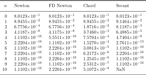
, we compare the iteration histories of Newton’s method, Newton’s method with a forward difference derivative, and the chord method. We will use both a table and a plot, and invite the reader to pick her or his own favourite way to present such data.
To illustrate the effects of the error in
 $f$
, we tabulate and plot
 $|f|$
for the three methods. We set the termination criteria to
 $\unicode[STIX]{x1D70F}_{a}=\unicode[STIX]{x1D70F}_{r}=10^{-20}$
. Since
 $\unicode[STIX]{x1D716}\approx 10^{-15}$
in this example, the theory does not imply that it is possible to drive the residual to a value as small as
 $10^{-20}$
, and the computation confirms that. We used a difference increment of
 $h=10^{-7}$
.
Iteration histories:
 $|f(x_{n})|$
.

Those of you accustomed to looking at columns of figures may have noticed that, as the theory predicts, there is very little difference between the finite-difference Newton method and the version with analytic derivatives until the iteration stagnates at roughly the level of machine precision. One can also notice that the residuals for the chord method decay more slowly, by a factor of 4–5 with each iteration. The secant method converges faster than chord, but not as fast as Newton’s method. One weakness of the secant method is exposed by the
 $10$
th iteration, where there is a floating-point exception. The problem is that the
 $f(x_{n})=f(x_{n+1})$
and
 $x_{n}=x_{n+1}$
at this point, so one gets
 $j_{c}=0/0$
, which is reported in IEEE arithmetic (Overton Reference Overton2001) as NaN (Not a Number). In this example we have run the iteration far beyond any sensible termination point. The NaN and the stagnation in the Newton iteration are signs of that.
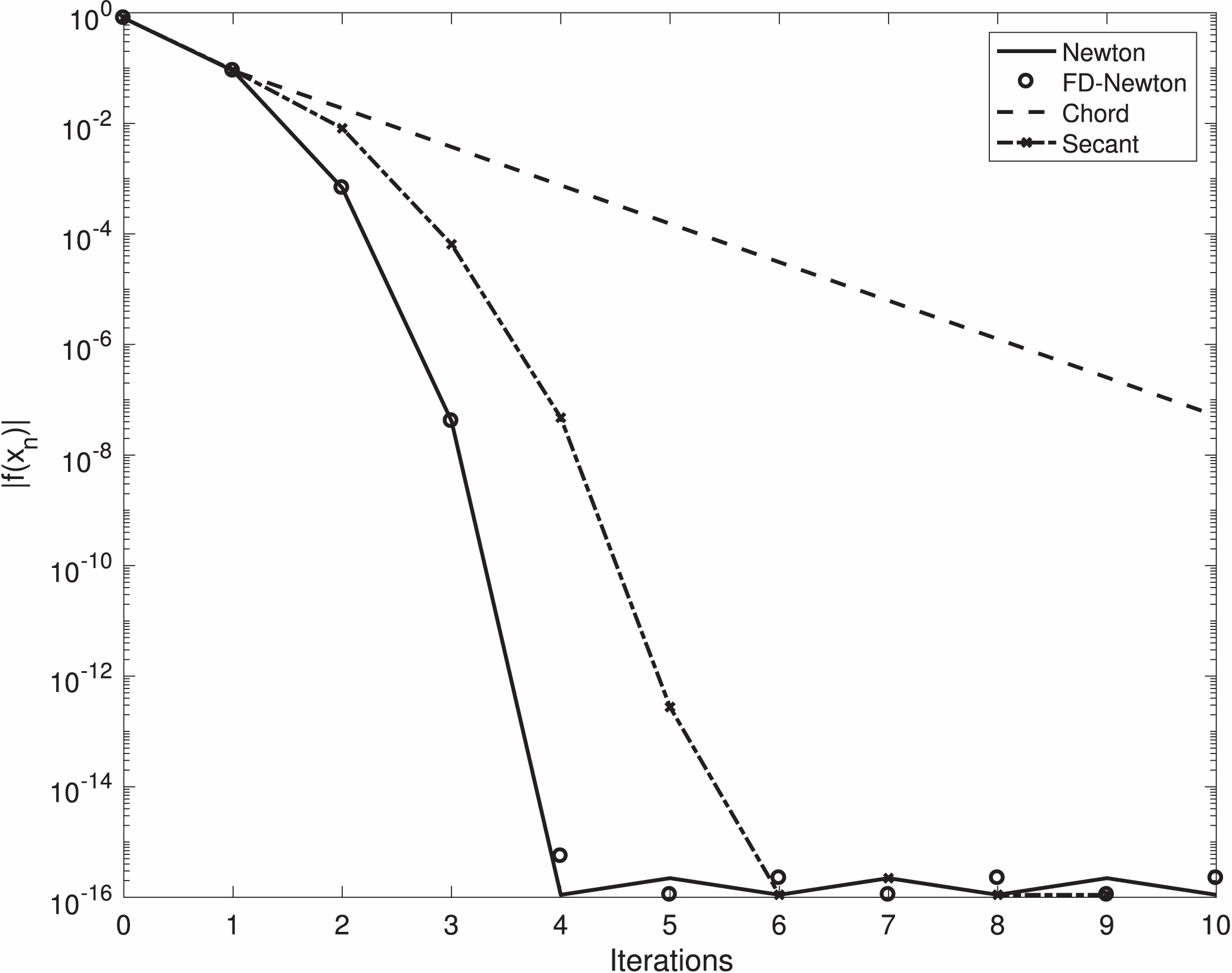
It is more illuminating, at least in the author’s opinion, to visualize iteration histories, and Table 2.1 is one of the very few tables we will use for that. In Figure 2.1 we visualize the data from the table in a semi-log plot. It is very clear that there is little difference between the two realizations of Newton’s method in terms of the number of nonlinear iterations needed to converge to the limiting level of precision. One can also see the signature of superlinear convergence in downward concavity of the residual history for Newton’s method and the secant method. The NaN is missing from the plot by convention. The q-linear convergence of the chord method appears as a linear residual history when plotted in this way.
Visual iteration histories.

As a general rule, if residuals are accurate to machine unit roundoff, the iterations will stagnate at that level. There are exceptions. For example, if the floating-point implementation of a function has a root in the floating-point number system, then one can continue the iteration for much longer. The equation
 $\arctan (x)=0$
is an example of this phenomenon.
Our final example in this section is the Shamanskii method (Shamanskii Reference Shamanskii1967). This method is a hybrid between Newton’s method and the chord method. The idea is to update the Jacobian every
 $m\geq 1$
iterations. Clearly
 $m=1$
is Newton’s method and
 $m=\infty$
is the chord method. If Gaussian elimination is the linear solver, the Shamanskii iteration for finite
 $m$
is
shamanskii_LU.
In algorithm shamanskii_LU the iteration counter is incremented outside of the inner
 $j$
loop. Keeping this in mind, Theorem 2.3 states that
 $$\begin{eqnarray}\Vert \mathbf{e}_{n+1}\Vert =O(\Vert \mathbf{e}_{n}\Vert ^{m+1}).\end{eqnarray}$$
If
 $m>1$
the convergence rate is faster than the q-quadratic rate for Newton’s method. We say the convergence is q-superlinear with q-order
 $m+1$
. The Shamanskii method is less appealing than it appears because if the Jacobian is sufficiently near
 $\mathbf{F}^{\prime }(\mathbf{x}^{\ast })$
the modest reduction in the iterations is not worth the cost of computing and factoring the Jacobian. In many cases
 $m=\infty$
(the chord method) is a better choice (Brent Reference Brent1973).
This section has looked at the effects of
 $\unicode[STIX]{x1D6E5}$
and
 $\unicode[STIX]{x1D716}$
on the convergence of Newton’s method. Typically proofs set
 $\unicode[STIX]{x1D716}=0$
and proceed as if evaluations
 $\mathbf{F}$
were exact. The users of the results generally know that
 $\unicode[STIX]{x1D716}\neq 0$
and when the error in the function evaluation is important. We will follow that approach in the next section, where the inexactness in the linear solver, measured by
 $\unicode[STIX]{x1D702}$
, is the important part of the algorithm.

2.6 Inexact Newton methods and JFNK
When one solves a linear equation
 $\mathbf{A}\mathbf{x}=\mathbf{b}$
with an iterative method, one usually terminates the iteration when the relative residual
 $\Vert \mathbf{A}\mathbf{x}-\mathbf{b}\Vert /\Vert \mathbf{b}\Vert$
is sufficiently small. An inexact Newton method (Dembo et al.
Reference Dembo, Eisenstat and Steihaug1982) approximates Newton’s method by using a step
 $\mathbf{s}$
that satisfies the inexact Newton condition
 $$\begin{eqnarray}\Vert \mathbf{F}^{\prime }(\mathbf{x}_{c})\mathbf{s}+\mathbf{F}(\mathbf{x}_{c})\Vert \leq \unicode[STIX]{x1D702}_{c}\Vert \mathbf{F}(\mathbf{x}_{c})\Vert .\end{eqnarray}$$
Here
 $\unicode[STIX]{x1D702}$
is called the forcing term.
While the theory does not say how one realizes (2.19), in practice it is usually the outcome of an iterative method for solving
 $\mathbf{F}^{\prime }(\mathbf{x}_{c})\mathbf{x}=-\mathbf{F}(\mathbf{x}_{c})$
. The term Newton-iterative method is used in that case. The iteration for
 $\mathbf{x}$
is called the outer or nonlinear iteration. The iterative method for the linear equation is called the inner or linear iteration. A specific linear solver or class of solvers is often specified. For example Newton–Krylov and Newton–GMRES are common choices. Preconditioners can also be part of the name. Newton–Krylov–Schwarz (Cai, Gropp, Keyes and Tidriri Reference Cai, Gropp, Keyes, Tidriri and Rannacher1994) methods use a Krylov linear solver and a Schwarz domain decomposition method as a preconditioner.
A straightforward application of Theorem 2.3 with
 $\unicode[STIX]{x1D6E5}=0$
and
 $\unicode[STIX]{x1D716}=0$
leads to
 $$\begin{eqnarray}\Vert \mathbf{e}_{+}\Vert =O(\Vert \mathbf{e}_{c}\Vert ^{2}+\unicode[STIX]{x1D702}_{c}\Vert \mathbf{e}_{c}\Vert ).\end{eqnarray}$$
The estimate (2.20) leads to a convergence theorem.
Theorem 2.4. Let Assumption 2.1 hold. Then if
 $\mathbf{x}_{0}$
is sufficiently near
 $\mathbf{x}^{\ast }$
,
 $0\leq \unicode[STIX]{x1D702}_{n}\leq \bar{\unicode[STIX]{x1D702}}<1$
, and
 $\bar{\unicode[STIX]{x1D702}}$
is sufficiently small, then inexact Newton iteration converges. Moreover, the convergence is
∙ q-linear,
∙ q-superlinear if
$\unicode[STIX]{x1D702}_{n}\rightarrow 0$
, and∙ q-quadratic if
$\unicode[STIX]{x1D702}_{n}=O(\Vert \mathbf{F}(\mathbf{x}_{n})\Vert )$
.


There are, as one might suspect from Theorem 2.4, many approaches to managing
 $\unicode[STIX]{x1D702}$
as the iteration progresses. Similar to the distinction between Newton’s method and the chord method, it is rarely a good idea to make
 $\unicode[STIX]{x1D702}$
very small, especially at the beginning of the iteration when only limited accuracy is needed to get the same reduction in error that one would get with Newton’s method itself. While one could make
 $\unicode[STIX]{x1D702}$
small once the residuals are small, it is not clear that the additional cost in the linear solve makes the reduction in nonlinear iterations worthwhile. There are useful discussions of this issue in Kelley (Reference Kelley1995) and Eisenstat and Walker (Reference Eisenstat and Walker1996). The author of this article has had success with
 $\unicode[STIX]{x1D702}_{n}\equiv 1/10$
.
Theorem 2.4 does not specify any particular norm. If one uses the weighed norm
 $$\begin{eqnarray}\Vert \mathbf{x}\Vert _{\ast }=\Vert \mathbf{F}^{\prime }(\mathbf{x}^{\ast })\mathbf{x}\Vert ,\end{eqnarray}$$
then the theory no longer needs a small
 $\bar{\unicode[STIX]{x1D702}}$
. Any
 $\bar{\unicode[STIX]{x1D702}}<1$
will do.
Theorem 2.5. Let Assumption 2.1 hold. Then if
 $\mathbf{x}_{0}$
is sufficiently near
 $\mathbf{x}^{\ast }$
and
 $0\leq \unicode[STIX]{x1D702}_{n}\leq \bar{\unicode[STIX]{x1D702}}<\tilde{\unicode[STIX]{x1D702}}<1$
,
 $$\begin{eqnarray}\Vert \mathbf{e}_{n+1}\Vert _{\ast }\leq \tilde{\unicode[STIX]{x1D702}}\Vert \mathbf{e}_{n}\Vert _{\ast }\end{eqnarray}$$
and the other conclusions of Theorem 2.4 hold.
Assuming that
 $\mathbf{e}_{n}\neq 0$
for all
 $n$
, Theorem 2.5 implies that
 $$\begin{eqnarray}\limsup \displaystyle \frac{\Vert \mathbf{e}_{n+1}\Vert _{\ast }}{\Vert \mathbf{e}_{n}\Vert _{\ast }}\leq \bar{\unicode[STIX]{x1D702}}.\end{eqnarray}$$
If the linear solver is a Krylov method which only needs Jacobian-vector products, it is not necessary or desirable to compute and store a Jacobian matrix. For example, one can approximate the Jacobian-vector product with a forward difference. Methods of this type are called Jacobian-free Newton–Krylov (JFNK) methods. JFNK methods are the most common choice for those large-scale nonlinear equations which come from differential and integral equations. Knoll and Keyes (Reference Knoll and Keyes2004) provide an excellent account of JNFK methods and applications.
The linear solver in a JFNK method often requires preconditioning to work well enough to be useful. In most implementations preconditioning is done at the level of the linear solver. Preconditioning can also be encoded in the nonlinear map itself and it is interesting to examine that. We will let
 $\mathbf{M}$
be the preconditioner for the linear equation for the Newton step, and assume that
 $\mathbf{M}$
does not depend on the
 $\mathbf{x}$
, the nonlinear iteration. If we precondition from the left, the equation for the Newton step is transformed into
 $$\begin{eqnarray}\mathbf{M}\mathbf{F}^{\prime }(\mathbf{x}_{c})\mathbf{s}=-\mathbf{M}\mathbf{F}(\mathbf{x}_{c}).\end{eqnarray}$$
This is exactly the Newton step for the equation
 $$\begin{eqnarray}\mathbf{M}\mathbf{F}(\mathbf{x})=0.\end{eqnarray}$$
So, in the case of left preconditioning, one can place the preconditioning in the definition of the nonlinear map, replacing
 $\mathbf{F}$
by
 $\mathbf{M}\mathbf{F}$
, or apply it to the linear equation for the step. In either case, the steps and the iterations will be the same as in the unpreconditioned case. Most of the production codes put the preconditioning in the linear solve and measure the unpreconditioned residual
 $\mathbf{F}$
when terminating the linear iteration. When one does this, however, the termination criterion for the linear iteration would be
 $$\begin{eqnarray}\Vert \mathbf{M}\mathbf{F}^{\prime }(\mathbf{x}_{c})\mathbf{s}+\mathbf{M}\mathbf{F}(\mathbf{x}_{c})\Vert \leq \unicode[STIX]{x1D702}\Vert \mathbf{M}\mathbf{F}(\mathbf{x}_{c})\Vert ,\end{eqnarray}$$
which is the inexact Newton condition for
 $\mathbf{M}\mathbf{F}$
. This does not change the theory if
 $\unicode[STIX]{x1D702}$
is sufficiently small. To summarize, replacing
 $\mathbf{F}$
with
 $\mathbf{M}\mathbf{F}$
does not change the iteration or the steps, but does change the norm of the Jacobian at the solution and the Lipschitz constant for the Jacobian.
Similarly, if one preconditions the linear equation from the right, the equation is
 $$\begin{eqnarray}\mathbf{F}^{\prime }(\mathbf{x}_{c})\mathbf{M}\mathbf{z}=-\mathbf{F}(\mathbf{x}_{c}),\quad \mathbf{s}=\mathbf{M}\mathbf{z},\end{eqnarray}$$
and the corresponding nonlinear system is
 $$\begin{eqnarray}\mathbf{F}(\mathbf{M}\mathbf{y})=0,\quad \mathbf{x}=\mathbf{M}\mathbf{y}.\end{eqnarray}$$
In this case the residuals are unchanged and the inexact Newton condition has its original meaning if one puts the preconditioning in the linear solver.
2.7 Global convergence
The Newton iteration for
 $\arctan (x)=0$
with
 $x_{0}=1$
exhibits classic quadratic convergence. With a poor initial iterate,
 $x_{0}=10$
for example, the first five iterations are
 $$\begin{eqnarray}10,\quad -138,\quad 2.9\times 10^{4},\quad -1.5\times 10^{9},\quad 9.9\times 10^{17}.\end{eqnarray}$$
This divergence is consistent with the theory because the initial iterate is so poor. The Armijo line search (Armijo Reference Armijo1966) is a wonderful and simple solution to this problem.
The idea is to observe that even though the Newton step moves farther from the root, the direction is correct. To clarify this we make a distinction between the Newton direction
 $$\begin{eqnarray}\mathbf{d}=-\mathbf{F}^{\prime }(\mathbf{x}_{c})^{-1}\mathbf{F}(\mathbf{x}_{c})\end{eqnarray}$$
and the Newton step
 $$\begin{eqnarray}\mathbf{s}=\mathbf{x}_{+}-\mathbf{x}_{c}.\end{eqnarray}$$
The simplest strategy is to find the least
 $\unicode[STIX]{x1D706}=2^{-m}$
for
 $m=0,1,\ldots \,$
so that
 $$\begin{eqnarray}\Vert \mathbf{F}(\mathbf{x}_{c}+\unicode[STIX]{x1D706}\mathbf{d})\Vert <\Vert \mathbf{F}(\mathbf{x}_{c})\Vert\end{eqnarray}$$
and use
 $\mathbf{s}=\unicode[STIX]{x1D706}\mathbf{d}$
. The simple decrease condition (2.21) is a bit too weak for a convergence analysis, but is close enough to save the
 $\arctan$
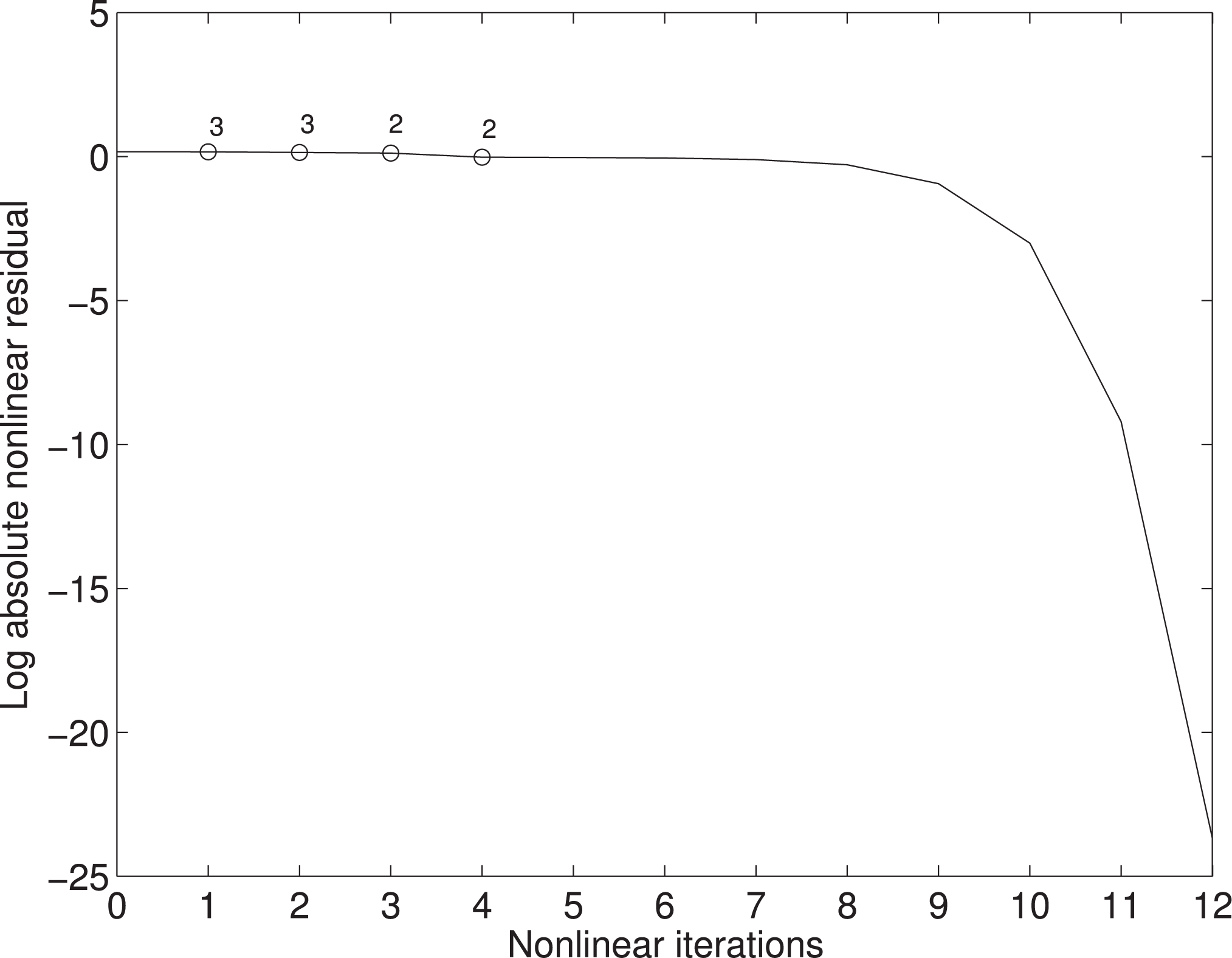
iteration, as one can see in Figure 2.2.
The Armijo line search for
 $\arctan (x)=0$
,
 $x_{0}=10$
.

In the figure the circles are iterations for which the step length required reduction, and the number of stepsize reductions are indicated next to the circles. After the fourth iteration the iteration took full steps, and the local theory holds. Note that the residual reduction continued past the resolution of the floating-point system. The reason for this, as we mentioned in Section 2.5, is that
 $x^{\ast }=0$
is also a solution of the equation as implemented in MATLAB with IEEE floating-point arithmetic.
Convergence theory requires more than simple decrease as in (2.21). The sufficient decrease condition that one needs for theory is
 $$\begin{eqnarray}\Vert \mathbf{F}(\mathbf{x}_{c}+2^{-m}\mathbf{d})\Vert <(1-\unicode[STIX]{x1D6FC}2^{-m})\Vert \mathbf{F}(\mathbf{x}_{c})\Vert .\end{eqnarray}$$
In most of the literature and codes,
 $\unicode[STIX]{x1D6FC}=10^{-4}$
. In most cases sufficient decrease conditions such as (2.22) will lead to the same stepsize decisions as simple decrease, and the purpose is to enable theory. It is common to adaptively change the stepsize reduction factor. One way to do this (Kelley Reference Kelley1995, Dennis and Schnabel Reference Dennis and Schnabel1996) is to begin with a stepsize of
 $\unicode[STIX]{x1D706}=1$
, and with each failure of the sufficient decrease condition
 $$\begin{eqnarray}\Vert \mathbf{F}(\mathbf{x}_{c}+\unicode[STIX]{x1D706}\mathbf{d})\Vert <(1-\unicode[STIX]{x1D6FC}\unicode[STIX]{x1D706})\Vert \mathbf{F}(\mathbf{x}_{c})\Vert ,\end{eqnarray}$$
reduce
 $\unicode[STIX]{x1D706}$
by a factor
 $\unicode[STIX]{x1D70E}\in [0.1,0.5]$
. The standard way to do this is to use this history of failed steps to generate a polynomial approximation of
 $\unicode[STIX]{x1D719}(\unicode[STIX]{x1D706})=\Vert \mathbf{F}(\mathbf{x}_{c}+\unicode[STIX]{x1D706}\mathbf{d})\Vert$
and minimize that polynomial. This adaptivity is very useful in practice.
Algorithm newton_armijo is an inexact formulation of the Newton–Armijo method. It includes the essential ideas and makes the theory easy to state. It is critical that one uses
 $\mathbf{F}^{\prime }(\mathbf{x})$
and not an approximation. The Armijo rule is not, for example, theoretically supported for the chord method. Adding a line search to a Newton code is easy and requires only a few new lines.

Algorithm newton_armijo does not say how or if the forcing term
 $\unicode[STIX]{x1D702}$
changes with the iteration. Most of the codes do vary
 $\unicode[STIX]{x1D702}$
and use the ideas in Eisenstat and Walker (Reference Eisenstat and Walker1996). One example from Eisenstat and Walker (Reference Eisenstat and Walker1996) which is common is
 $$\begin{eqnarray}\unicode[STIX]{x1D702}_{n}=\left\{\begin{array}{@{}ll@{}}\unicode[STIX]{x1D702}_{\max }\quad & n=0,\\ \min (\unicode[STIX]{x1D702}_{\max },\unicode[STIX]{x1D702}_{n}^{A})\quad & n>0.\end{array}\right.\end{eqnarray}$$
Here
 $$\begin{eqnarray}\unicode[STIX]{x1D702}_{n}^{A}=\unicode[STIX]{x1D6FE}_{\unicode[STIX]{x1D702}}\Vert F(x_{n})\Vert ^{2}/\Vert F(x_{n-1})\Vert ^{2}\end{eqnarray}$$
and
 $\unicode[STIX]{x1D6FE}_{\unicode[STIX]{x1D702}}$
is a parameter. The parameter
 $\unicode[STIX]{x1D702}_{\max }$
is an upper limit on the sequence
 $\{\unicode[STIX]{x1D702}_{n}\}$
. Eisenstat and Walker (Reference Eisenstat and Walker1996) use the choices
 $\unicode[STIX]{x1D6FE}_{\unicode[STIX]{x1D702}}=0.9$
and
 $\unicode[STIX]{x1D702}_{\max }=0.9999$
. The author of this article, however, likes the choice
 $\unicode[STIX]{x1D702}_{n}\equiv 0.1$
.
Theorem 2.6 is very satisfying. For sufficiently smooth problems, the Newton–Armijo iteration has only three possible outcomes. One is convergence to a solution which satisfies the standard assumptions. In that case the stepsize
 $\unicode[STIX]{x1D706}$
will be one in the terminal phase of the iteration. The other two outcomes are failures, which are easy to detect numerically. One failure mode is that the iteration becomes unbounded. An example of such a problem is the scalar equation
 $e^{x}=0$
, where the Newton–Armijo iteration diverges to
 $-\infty$
. The second failure mode is that the Jacobian drifts to singularity. An example is the scalar equation
 $x^{2}+1=0$
.
Theorem 2.6. Suppose
 $\mathbf{F}$
is Lipschitz continuously differentiable,
 $\{\mathbf{x}_{n}\}$
is the inexact Newton–Armijo sequence, and
 $0<\unicode[STIX]{x1D702}_{n}<\bar{\unicode[STIX]{x1D702}}<1$
. Then there are only three possibilities.
∙
$\{\mathbf{x}_{n}\}$
converges to a root
$\mathbf{x}^{\ast }$
of
$\mathbf{F}$
at which the standard assumptions hold, full steps (
$\unicode[STIX]{x1D706}=1$
) are taken for
$n$
sufficiently large, and the local convergence theory holds.∙ The sequence
$\{\mathbf{x}_{n}\}$
is unbounded.∙ The sequence
$\{\mathbf{F}^{\prime }(\mathbf{x}_{n})^{-1}\}$
is unbounded.


The Newton–Armijo method does not solve all problems. Even in the successful case, there is no guarantee that the iteration converges to a useful solution. Nonlinear equations can have multiple solutions, and there are often constraints such as dynamic stability or correct signs for physical quantities to which the Newton iteration is oblivious. We will consider a few ways to address non-uniqueness in Sections 4 and 7.
Another approach to globalization is that of trust region methods (Powell Reference Powell and Rabinowitz1970). These methods are widely used in optimization (Conn, Gould and Toint Reference Conn, Gould and Toint2000), but less so for nonlinear equations. The idea is to model
 $\Vert \mathbf{F}(\mathbf{x}_{c})\Vert _{2}^{2}$
with a quadratic and minimize that quadratic in a bounded set, the trust region, centred at
 $x_{c}$
. We will not discuss these methods in detail here. Absil, Baker and Gallivan (Reference Absil, Baker and Gallivan2007) and Higham (Reference Higham1999) report on some interesting applications which are connected to the continuation methods in Section 7.
2.8 Broyden’s method
Quasi-Newton methods construct a model Jacobian from the history of the iteration. One maintains both an approximation
 $\mathbf{x}_{n}$
of the solution and an approximation
 $\mathbf{B}_{n}$
of the Jacobian. There are many of these methods (Kelley Reference Kelley1995, Dennis and Schnabel Reference Dennis and Schnabel1996, Dennis and Walker Reference Dennis and Walker1981) and they are widely used in optimization. They have largely been replaced by JFNK methods for nonlinear equations. We will briefly discuss Broyden’s method, the simplest of them and the one that is used in the NOX code from Trilinos (Heroux et al.
Reference Heroux, Bartlett, Howle, Hoekstra, Hu, Kolda, Lehoucq, Long, Pawlowski, Phipps, Salinger, Thornquist, Tuminaro, Willenbring, Williams and Stanley2005).
The Broyden update is
 $$\begin{eqnarray}\mathbf{B}_{+}=\mathbf{B}_{c}+{\displaystyle \frac{(\mathbf{y}-\mathbf{B}_{c}\mathbf{s})\mathbf{s}^{T}}{\mathbf{s}^{T}\mathbf{s}}}.\end{eqnarray}$$
Here
 $\mathbf{y}=\mathbf{F}(\mathbf{x}_{+})-\mathbf{F}(\mathbf{x}_{c})$
and
 $\mathbf{s}=\mathbf{x}_{+}-\mathbf{x}_{c}$
. One can think of this as a generalization of the secant method for scalar equations. For the secant equation, the model derivative at the new point
 $x_{+}$
is
 $$\begin{eqnarray}b_{+}=\displaystyle \frac{f(x_{+})-f(x_{c})}{x_{+}-x_{c}}=\displaystyle \frac{y}{s},\end{eqnarray}$$
giving
 $b_{+}s=y$
. For systems of equations, the secant equation
 $$\begin{eqnarray}\mathbf{B}_{+}\mathbf{s}=\mathbf{y}\end{eqnarray}$$
is a system of
 $N$
equations in
 $N^{2}$
unknowns. This enables construction of updates that satisfy structural constraints such as sparsity or positivity. Dennis and Schnabel (Reference Dennis and Schnabel1996) and Kelley (Reference Kelley1995) discuss several kinds of secant updates for nonlinear equations. In optimization, for example, one often wants the model Hessian to be symmetric and positive definite. There are many quasi-Newton update which do that (Dennis and Schnabel Reference Dennis and Schnabel1996, Kelley Reference Kelley1999, Nocedal and Wright Reference Nocedal and Wright1999). One can also design updates to capture functional analytic properties of infinite-dimensional problems and their discretizations (Kelley and Sachs Reference Kelley and Sachs1993, Kelley and Sachs Reference Kelley and Sachs1995, Kelley and Sachs Reference Kelley and Sachs1987, Kelley and Sachs Reference Kelley and Sachs1989, Hart and Soul Reference Hart and Soul1973). The most general accounts of theory can be found in Dennis and Walker (Reference Dennis and Walker1981) and Dennis and Schnabel (Reference Dennis and Schnabel1979).
One can implement the Broyden update by storing two vectors for each iteration and using the Sherman–Morrison formula (Kelley Reference Kelley1995) to update the product of
 $\mathbf{B}^{-1}$
and a vector. The storage burden can be reduced to one vector per nonlinear iteration by using the dependence of
 $\mathbf{y}$
on
 $\mathbf{s}$
(Kelley Reference Kelley1995, Deuflhard, Freund and Walter Reference Deuflhard, Freund and Walter1990). JFNK methods place the storage burden on the linear iteration, and that seems to be best.
The formula for the update (2.25) allows for a line search in which
 $$\begin{eqnarray}\mathbf{s}=-\unicode[STIX]{x1D706}\mathbf{B}_{c}^{-1}\mathbf{F}(\mathbf{x}_{c}).\end{eqnarray}$$
Theorem 2.6 does not apply to a Broyden–Armijo algorithm patterned after algorithm newton_armijo, but in practice such an algorithm often works fine.
The convergence theory is only local and requires the standard assumptions and accurate initial approximations to the solution and the Jacobian at the solution.
Theorem 2.7. If the standard assumptions hold and
 $\mathbf{x}_{0}$
and
 $\mathbf{B}_{0}$
are sufficiently near
 $\mathbf{x}^{\ast }$
and
 $\mathbf{F}^{\prime }(\mathbf{x}^{\ast })$
, then
 $\mathbf{x}_{n}\rightarrow \mathbf{x}^{\ast }$
q-superlinearly:
 $$\begin{eqnarray}\lim _{n\rightarrow \infty }\displaystyle \frac{\Vert \mathbf{e}_{n+1}\Vert }{\Vert \mathbf{e}_{n}\Vert }=0.\end{eqnarray}$$
Broyden’s method and JFNK methods have remarkable similarities when applied to discretizations of infinite-dimensional problems. The preconditioning issues are very closely related; see, for example, Kelley and Sachs (Reference Kelley and Sachs1985), Kelley and Xue (Reference Kelley and Xue1996), Burmeister (Reference Burmeister1975) and Nevanlinna (Reference Nevanlinna1993).
2.9 Fréchet and Gâteaux derivatives
We have not fully explained how the results in this section map to the infinite-dimensional setting. The reason for this is that we have defined the derivative in the context of its matrix representation as a Jacobian matrix. We are now at a point where we must make a coordinate-free definition to consider our first infinite-dimensional example in the next section.
If
 $D\subset \mathbb{R}^{M}$
, we will let
 $D^{\circ }$
denote the interior of
 $D$
.
Definition 2.8. A function
 $\mathbf{F}:D\subset \mathbb{R}^{N}\rightarrow \mathbb{R}^{M}$
is Fréchet differentiable at
 $x\in D^{\circ }$
if there is a linear map
 $\mathbf{F}^{\prime }(\mathbf{x})$
from
 $\mathbb{R}^{M}$
to
 $\mathbb{R}^{N}$
such that
 $$\begin{eqnarray}\lim _{\mathbf{h}\rightarrow 0}\displaystyle \frac{\Vert \mathbf{F}(\mathbf{x}+\mathbf{h})-\mathbf{F}(\mathbf{x})-\mathbf{F}^{\prime }(\mathbf{x})\mathbf{h}\Vert }{\Vert \mathbf{h}\Vert }=0.\end{eqnarray}$$
 $\mathbf{F}^{\prime }$
is called the Fréchet derivative (or simply the derivative) of
 $\mathbf{F}$
at
 $\mathbf{x}$
.
Fréchet differentiability simply means that the difference quotients converge to the derivative uniformly in the direction
 $\mathbf{h}/\Vert \mathbf{h}\Vert$
as
 $\Vert \mathbf{h}\Vert \rightarrow 0$
. The Jacobian matrix is simply the matrix representation of the Fréchet derivative in the basis of coordinate directions. So the
 $j$
th column of the Jacobian is
 $\mathbf{F}^{\prime }(\mathbf{x})\mathbf{u}_{j}$
as expressed in (2.11). The results on convergence of Newton’s method in this section do not change in the infinite-dimensional case. For quasi-Newton methods, such as Broyden’s method, superlinear convergence depends on compactness properties (Kelley and Sachs Reference Kelley and Sachs1985) of
 $\mathbf{I}-{\mathcal{F}}^{\prime }$
, which are trivially satisfied in finite-dimensional problems.
One useful way to compute the Fréchet derivative is to apply (2.26) to compute
 $\mathbf{F}^{\prime }(\mathbf{x})\mathbf{u}$
for an arbitrary
 $\mathbf{u}$
. Often one can easily extract
 $\mathbf{F}^{\prime }$
directly by looking at the results, since
 $$\begin{eqnarray}\mathbf{F}^{\prime }(\mathbf{x})\mathbf{u}=\displaystyle \frac{\text{d}}{\,\text{d}t}\mathbf{F}(\mathbf{x}+t\mathbf{u})\bigg|_{t=0}.\end{eqnarray}$$
As an example, suppose that
 $$\begin{eqnarray}\mathbf{F}(\mathbf{x})=\mathbf{A}\mathbf{x}+f(\mathbf{x}),\end{eqnarray}$$
where
 $\mathbf{A}$
is a linear operator and
 $f(\mathbf{x})$
is the substitution operator
 $$\begin{eqnarray}f(\mathbf{x})\equiv \left(\begin{array}{@{}c@{}}f(x_{1})\\ f(x_{2})\\ \vdots \\ f(x_{N})\end{array}\right)\!.\end{eqnarray}$$
Then (2.27) implies that
 $$\begin{eqnarray}\mathbf{F}^{\prime }(\mathbf{x})=\mathbf{A}+\text{diag}(f^{\prime }(\mathbf{x})).\end{eqnarray}$$
If it exists, the limit
 $$\begin{eqnarray}\,\text{d}\mathbf{F}(\mathbf{x}:\mathbf{u})=\lim _{t\downarrow 0}\displaystyle \frac{\mathbf{F}(\mathbf{x}+t\mathbf{u})-\mathbf{F}(\mathbf{x})}{t}\end{eqnarray}$$
is called the directional derivative of
 $\mathbf{F}$
at
 $\mathbf{x}$
in the direction
 $\mathbf{u}$
. The scalar example
 $f(x)=|x|$
at
 $x=0$
has directional derivatives in all directions, but is not Fréchet differentiable. This example also shows that
 $\text{d}\mathbf{F}(\mathbf{x}:\mathbf{u})$
need not be linear in
 $\mathbf{u}$
. If the limit
 $$\begin{eqnarray}\,\text{d}\mathbf{F}(\mathbf{x}:\mathbf{u})=\lim _{t\rightarrow 0}\displaystyle \frac{\mathbf{F}(\mathbf{x}+t\mathbf{u})-\mathbf{F}(\mathbf{x})}{t}\end{eqnarray}$$
exists, then
 $\text{d}\mathbf{F}(\mathbf{x}:\mathbf{u})$
is called the Gâteaux derivative of
 $\mathbf{F}$
at
 $\mathbf{x}$
in the direction
 $\mathbf{u}$
. In this case
 $$\begin{eqnarray}\,\text{d}\mathbf{F}(\mathbf{x}:\mathbf{u})=\displaystyle \frac{\text{d}}{\,\text{d}t}\mathbf{F}(\mathbf{x}+t\mathbf{u})\bigg|_{t=0},\end{eqnarray}$$
but still need not be linear in
 $\mathbf{u}$
. With the exception of Sections 6 and 7.1, all functions in this article will be Fréchet differentiable. If
 $\mathbf{F}$
is Fréchet differentiable at
 $\mathbf{x}$
, then
 $\text{d}\mathbf{F}(\mathbf{x}:\mathbf{u})=\mathbf{F}^{\prime }(\mathbf{x})\mathbf{u}$
for all
 $\mathbf{u}$
.
2.10 Example: Chandrasekhar
$H$
-equation

This is the first example of an operator in a function space. We will denote such operators by script upper-case letters to distinguish them from their discretizations. The discretizations will be functions on
 $\mathbb{R}^{N}$
and will have the boldface fonts we have been using.
The Chandrasekhar
 $H$
-equation (Chandrasekhar Reference Chandrasekhar1960, Busbridge Reference Busbridge1960) is
 $$\begin{eqnarray}{\mathcal{F}}(H)(\unicode[STIX]{x1D707})=H(\unicode[STIX]{x1D707})-\biggl(1-{\displaystyle \frac{\unicode[STIX]{x1D714}}{2}}\displaystyle \int _{0}^{1}{\displaystyle \frac{\unicode[STIX]{x1D707}H(\unicode[STIX]{x1D708})\,\text{d}\unicode[STIX]{x1D708}}{\unicode[STIX]{x1D707}+\unicode[STIX]{x1D708}}}\biggr)^{-1}=0.\end{eqnarray}$$
The equation arises in radiative transfer theory and is a very tractable example of a nonlinear equation in a function space. We will regard
 ${\mathcal{F}}$
as a map on
 $C[0,1]$
, the Banach space of continuous function on the interval
 $[0,1]$
with the
 $\Vert \cdot \Vert _{\infty }$
-norm. The unknown is a function
 $H\in C[0,1]$
;
 $\unicode[STIX]{x1D714}\in [0,1]$
is a parameter.
We will discretize the equation with the composite midpoint rule
 $$\begin{eqnarray}\displaystyle \int _{0}^{1}f(\unicode[STIX]{x1D707})\,\text{d}\unicode[STIX]{x1D707}\approx \displaystyle \frac{1}{N}\mathop{\sum }_{j=1}^{N}f(\unicode[STIX]{x1D707}_{j}),\end{eqnarray}$$
where
 $\unicode[STIX]{x1D707}_{i}=(i-1/2)/N$
for
 $1\leq i\leq N$
.
This leads to an equation in
 $\mathbb{R}^{N}$
:
 $$\begin{eqnarray}\mathbf{F}^{N}(\mathbf{h})_{i}=h_{i}-\biggl(1-{\displaystyle \frac{\unicode[STIX]{x1D714}}{2N}}\mathop{\sum }_{j=1}^{N}{\displaystyle \frac{\unicode[STIX]{x1D707}_{i}h_{j}}{\unicode[STIX]{x1D707}_{i}+\unicode[STIX]{x1D707}_{j}}}\biggr)^{-1}.\end{eqnarray}$$
We will discuss some important properties of this equation in the context of the infinite-dimensional problem. Our conclusions will be equally valid for the discrete problem because the midpoint rule integrates constant functions exactly.
2.10.1 The continuous problem
Our first task is to differentiate
 ${\mathcal{F}}$
. Applying (2.26), we see that for all
 $v\in C[0,1]$
,
 $$\begin{eqnarray}({\mathcal{F}}^{\prime }(H)w)=w-\displaystyle \frac{\unicode[STIX]{x1D714}Lw}{(1-\unicode[STIX]{x1D714}LH)^{2}},\end{eqnarray}$$
where
 $L$
is the integral operator defined by
 $$\begin{eqnarray}Lw(\unicode[STIX]{x1D707})=\displaystyle \frac{1}{2}\int _{0}^{1}{\displaystyle \frac{\unicode[STIX]{x1D707}w(\unicode[STIX]{x1D708})\,\text{d}\unicode[STIX]{x1D708}}{\unicode[STIX]{x1D707}+\unicode[STIX]{x1D708}}}.\end{eqnarray}$$
Hence,
 $$\begin{eqnarray}{\mathcal{F}}^{\prime }(H)=I-\displaystyle \frac{\unicode[STIX]{x1D714}L}{(1-\unicode[STIX]{x1D714}LH)^{2}}.\end{eqnarray}$$
We will now check the standard assumptions. To see that there is a solution, we note that the sequence
 $$\begin{eqnarray}H_{0}=1,\quad H_{n+1}=1+\unicode[STIX]{x1D714}H_{n}LH_{n}\end{eqnarray}$$
is increasing. We will show convergence by showing that the
 $L^{1}$
-norms are bounded:
 $$\begin{eqnarray}\Vert H_{n}\Vert _{1}=\int _{0}^{1}H_{n}(\unicode[STIX]{x1D708})\,\text{d}\unicode[STIX]{x1D708}\leq \unicode[STIX]{x1D6FD}\equiv \displaystyle \frac{1+\sqrt{1-\unicode[STIX]{x1D714}}}{2/\unicode[STIX]{x1D714}}.\end{eqnarray}$$
Clearly (2.32) holds for
 $n=1$
. To proceed by induction, suppose
 $\Vert H_{n}\Vert _{1}\leq \unicode[STIX]{x1D6FD}$
. We seek to show that
 $$\begin{eqnarray}\int _{0}^{1}H_{n+1}(\unicode[STIX]{x1D707})\,\text{d}\unicode[STIX]{x1D707}=1+\displaystyle \frac{\unicode[STIX]{x1D714}}{2}\int _{0}^{1}\displaystyle \frac{\unicode[STIX]{x1D707}H_{n}(\unicode[STIX]{x1D708})H_{n}(\unicode[STIX]{x1D707})}{\unicode[STIX]{x1D707}+\unicode[STIX]{x1D708}}\,\text{d}\unicode[STIX]{x1D708}\end{eqnarray}$$
for all
 $0\leq \unicode[STIX]{x1D707}\leq 1$
. The trick is to integrate both sides of (2.33) with respect to
 $\unicode[STIX]{x1D707}$
and note that
 $$\begin{eqnarray}\displaystyle \int _{0}^{1}\int _{0}^{1}\displaystyle \frac{\unicode[STIX]{x1D707}H_{n}(\unicode[STIX]{x1D708})H_{n}(\unicode[STIX]{x1D707})}{\unicode[STIX]{x1D707}+\unicode[STIX]{x1D708}}\,\text{d}\unicode[STIX]{x1D708}\,\text{d}\unicode[STIX]{x1D707} & = & \displaystyle \int _{0}^{1}\int _{0}^{1}\displaystyle \frac{\unicode[STIX]{x1D708}H_{n}(\unicode[STIX]{x1D708})H_{n}(\unicode[STIX]{x1D707})}{\unicode[STIX]{x1D707}+\unicode[STIX]{x1D708}}\,\text{d}\unicode[STIX]{x1D708}\,\text{d}\unicode[STIX]{x1D707}\nonumber\\ \displaystyle & = & \displaystyle \Vert H_{n}\Vert _{1}^{2}/2\leq \unicode[STIX]{x1D6FD}^{2}/2.\nonumber\end{eqnarray}$$
We are done since
 $$\begin{eqnarray}\unicode[STIX]{x1D714}\unicode[STIX]{x1D6FD}^{2}/4+1\leq \unicode[STIX]{x1D6FD}\end{eqnarray}$$
by the quadratic formula. So our sequence
 $H_{n}$
converges in
 $L^{1}$
to a function
 $H$
which satisfies
 $H=1+\unicode[STIX]{x1D714}HLH$
. This implies that
 $H$
satisfies (2.30), since if
 $1-\unicode[STIX]{x1D714}LH$
vanishes at any
 $\unicode[STIX]{x1D707}\in [0,1]$
, then
 $H(\unicode[STIX]{x1D707})=1+H(\unicode[STIX]{x1D707})$
implying that
 $H(\unicode[STIX]{x1D707})=0$
, which violates the equation since
 $H(\unicode[STIX]{x1D707})\geq 1$
. Also, since
 $H_{n}$
is an increasing sequence,
 $H$
is a positive function of
 $\unicode[STIX]{x1D707}$
for
 $\unicode[STIX]{x1D714}\in [0,1]$
.
So
 $H\in L^{1}[0,1]$
satisfies (2.30). This implies that
 $H$
is continuous since
 $L$
is a bounded operator from
 $L^{1}[0,1]$
to
 $C[0,1]$
.
Lipschitz continuity of
 ${\mathcal{F}}^{\prime }$
is easy to check. The most interesting point is non-singularity of
 ${\mathcal{F}}^{\prime }(H)$
. If
 $H$
is the solution of (2.30), then it is clear by the argument above that
 $$\begin{eqnarray}\int _{0}^{1}H(\unicode[STIX]{x1D707})\,\text{d}\unicode[STIX]{x1D707}=\displaystyle \frac{1+\sqrt{1-\unicode[STIX]{x1D714}}}{2/\unicode[STIX]{x1D714}}.\end{eqnarray}$$
This clearly shows that there is no real solution for
 $\unicode[STIX]{x1D714}>1$
.
Since
 ${\mathcal{F}}^{\prime }$
is the sum of a compact integral operator and the identity, singularity of the operator implies that there is a non-trivial null space. Suppose
 ${\mathcal{F}}^{\prime }(H)w=0$
. Then
 $$\begin{eqnarray}w=\displaystyle \frac{\unicode[STIX]{x1D714}Lw}{(1-\unicode[STIX]{x1D714}LH)^{2}}.\end{eqnarray}$$
We may take
 $w\geq 0$
by the Perron–Frobenius theorem (Karlin Reference Karlin1959) and may therefore assume that
 $\int _{0}^{1}w(\unicode[STIX]{x1D707})\,\text{d}\unicode[STIX]{x1D707}>0$
. Since
 $H$
is a solution, we have
 $(1-\unicode[STIX]{x1D714}LH)^{-1}=H$
, and so
 $$\begin{eqnarray}w(1-\unicode[STIX]{x1D714}wLH)=\unicode[STIX]{x1D714}HLw.\end{eqnarray}$$
So
 $$\begin{eqnarray}\int _{0}^{1}w(\unicode[STIX]{x1D707})\,\text{d}\unicode[STIX]{x1D707}=\unicode[STIX]{x1D714}/2\int _{0}^{1}w(\unicode[STIX]{x1D707})\,\text{d}\unicode[STIX]{x1D707}\int _{0}^{1}H(\unicode[STIX]{x1D708})\,\text{d}\unicode[STIX]{x1D708}\end{eqnarray}$$
implies that
 $\unicode[STIX]{x1D714}\Vert H\Vert _{1}=2$
, which by (2.34) implies that
 $\unicode[STIX]{x1D714}=1$
.
So
 ${\mathcal{F}}^{\prime }(H)$
is non-singular unless
 $\unicode[STIX]{x1D714}=1$
. When
 $\unicode[STIX]{x1D714}=1$
,
 ${\mathcal{F}}^{\prime }(H)$
is indeed singular and, again by the Perron–Frobenius theorem, the null space has dimension one and is spanned by a non-negative function. In fact, that function is
 $w(\unicode[STIX]{x1D707})=\unicode[STIX]{x1D707}H(\unicode[STIX]{x1D707})$
. We see that the singularity structure of the
 $H$
-equation is quite simple and will use the
 $H$
-equation as an example again in Section 4.
2.10.2 The discrete problem
Now we return to the discrete version. The purpose of this section is to illustrate how exploiting problem structure can give very different cost estimates from the simple accounting of
 $O(N^{3})$
work for a linear solve and
 $N$
function evaluations for a Jacobian.
We begin with the cost of an evaluation. Using
 $\unicode[STIX]{x1D707}_{i}=(i-1/2)/N$
for
 $1\leq i\leq N$
and (2.31), we obtain
 $$\begin{eqnarray}\mathbf{F}^{N}(\mathbf{h})_{i}=h_{i}-\biggl(1-{\displaystyle \frac{\unicode[STIX]{x1D714}}{2N}}\mathop{\sum }_{j=1}^{N}{\displaystyle \frac{ih_{j}}{i+j-1}}\biggr)^{-1}.\end{eqnarray}$$
The approximate integral operator
 $\mathbf{L}$
, where
 $$\begin{eqnarray}\mathbf{L}_{ij}=\displaystyle \frac{\unicode[STIX]{x1D714}i}{2N(i+j-1)},\end{eqnarray}$$
is the product of a diagonal and a Hankel matrix (Golub and Van Loan Reference Golub and Van Loan1996). In fact
 $\mathbf{L}=\mathbf{D}_{1}\mathbf{K}$
, where
 $$\begin{eqnarray}\mathbf{D}_{1}=\text{diag}(i/2N)\end{eqnarray}$$
and
 $\mathbf{K}$
is the Hankel matrix
 $$\begin{eqnarray}\mathbf{K}_{ij}=1/(i+j-1).\end{eqnarray}$$
So evaluation of
 $\mathbf{L}\mathbf{h}$
can be done at a cost of
 $O(N\log N)$
work if one computes the product of the Hankel matrix and a vector with a fast Fourier transform (Golub and Van Loan Reference Golub and Van Loan1996). Since the remaining cost of the evaluation of
 $\mathbf{F}^{N}$
reduces to simple binary operations, the cost of a function evaluation is
 $O(N\log N)$
work.
We may now proceed exactly as we did in the continuous case. The Jacobian matrix is
 $$\begin{eqnarray}(\mathbf{F}^{N})^{\prime }(\mathbf{h})_{ij}=\unicode[STIX]{x1D6FF}_{ij}-\displaystyle \frac{\unicode[STIX]{x1D714}\mathbf{L}_{ij}}{1-\unicode[STIX]{x1D714}(\mathbf{L}\mathbf{u})_{i}}.\end{eqnarray}$$
Hence the Jacobian can be expressed as the identity plus the product of a diagonal and a Hankel matrix. If we set
 $$\begin{eqnarray}\mathbf{D}_{2}=\text{diag}(1-\unicode[STIX]{x1D714}(\mathbf{L}\mathbf{u})_{i})^{-1},\end{eqnarray}$$
then
 $$\begin{eqnarray}(\mathbf{F}^{N})^{\prime }(\mathbf{h})=\mathbf{I}=\unicode[STIX]{x1D714}\mathbf{D}_{1}\mathbf{D}_{2}\mathbf{K},\end{eqnarray}$$
and the Jacobian matrix can be constructed and stored with
 $O(N^{2})$
work and the Jacobian-vector product computed with
 $O(N\log N)$
work.
One conclusion that may be unexpected is that, even if one does the matrix–vector product with
 $\mathbf{K}$
naively for
 $O(N^{2})$
work, the solution with Newton–GMRES is far faster than one using a direct method to factor
 $\mathbf{F}^{\prime }$
. The integral equation structure can be exploited to show that the number of Krylov iterations per nonlinear iteration can be bounded independently of
 $N$
. Hence, as
 $N$
becomes large the advantage of Newton–Krylov over Newton–LU grows rapidly. The reader should try this and see. Chandrasekhar (Reference Chandrasekhar1960) tabulates the solution to several figures.
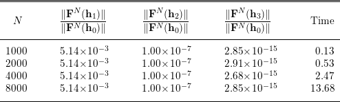
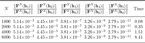
This problem has a rich structure and we will report the costs of a computation in some detail. Table 2.2 summarizes our discussion on the costs of function evaluations, Jacobian evaluations and Jacobian-vector products as functions of
 $N$
.
Iteration component costs.

We will now solve the
 $H$
-equation for a few values of
 $\unicode[STIX]{x1D714}$
. The problem becomes more difficult as
 $\unicode[STIX]{x1D714}$
increases. We will use
 $\unicode[STIX]{x1D714}=0.5$
(easy),
 $\unicode[STIX]{x1D714}=0.99$
(less easy) and
 $\unicode[STIX]{x1D714}=1$
(tricky). The initial iterate in all cases will be
 $$\begin{eqnarray}\mathbf{h}_{0}=(1,1,\ldots ,1)^{T}.\end{eqnarray}$$
We will terminate the iteration when
 $$\begin{eqnarray}\Vert \mathbf{F}^{N}(\mathbf{h}_{n})\Vert \leq 10^{-10}\Vert \mathbf{F}^{N}(\mathbf{h}_{0})\Vert ,\end{eqnarray}$$
so
 $\unicode[STIX]{x1D70F}_{r}=10^{-10}$
and
 $\unicode[STIX]{x1D70F}_{a}=0$
. We will use a mesh with
 $N=1000$
points to begin with and then demonstrate that the performance of all the methods does not vary much as the mesh is refined. We will do this numerically in this chapter and discuss the theory in Section 3.3.
We will first look at Newton’s method. The dominant cost for a Newton iteration is the matrix factorization. Therefore Newton’s method, even though the number of nonlinear iterations is small, is the most expensive approach for this problem when
 $\unicode[STIX]{x1D714}<1$
and the number of mesh points
 $N$
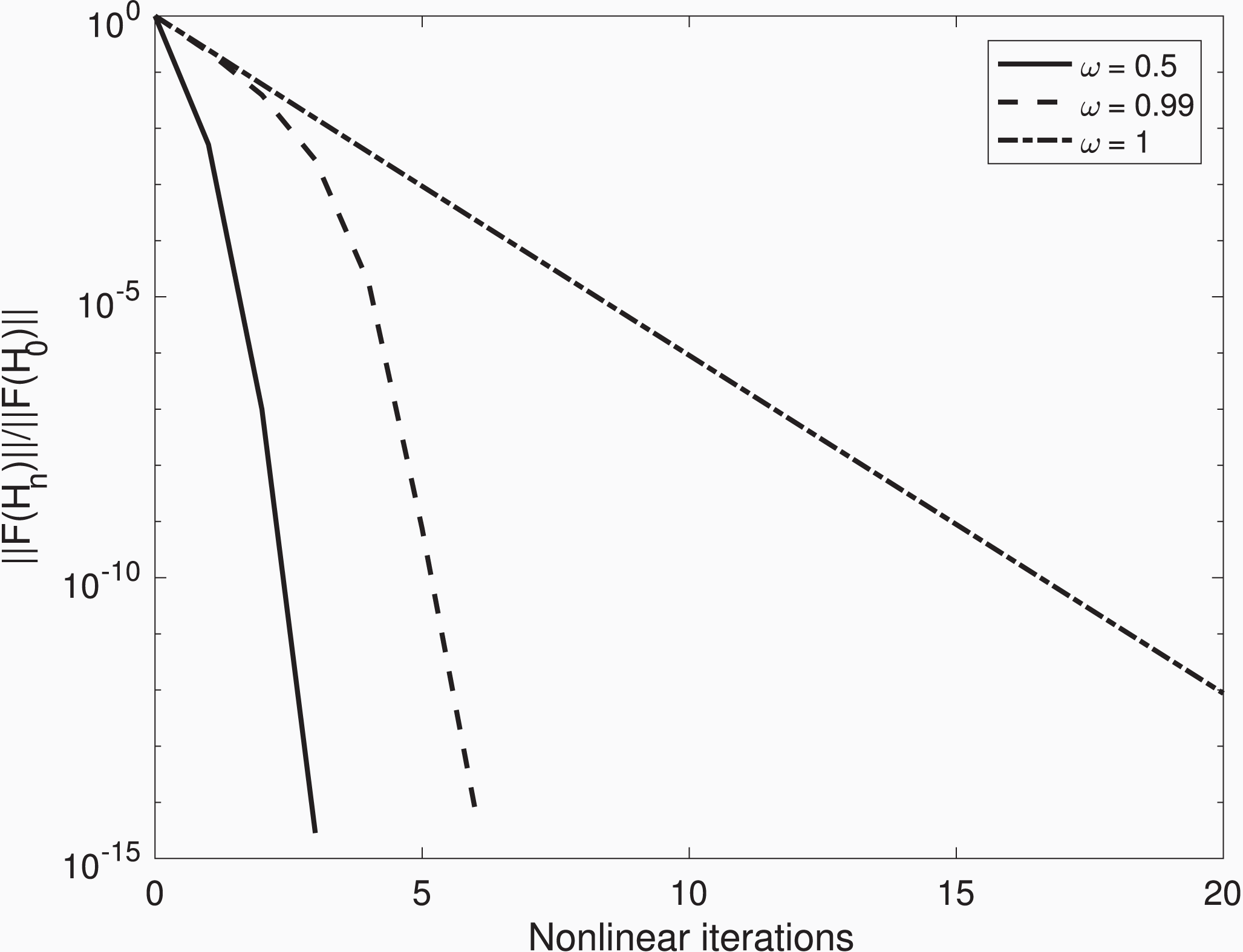
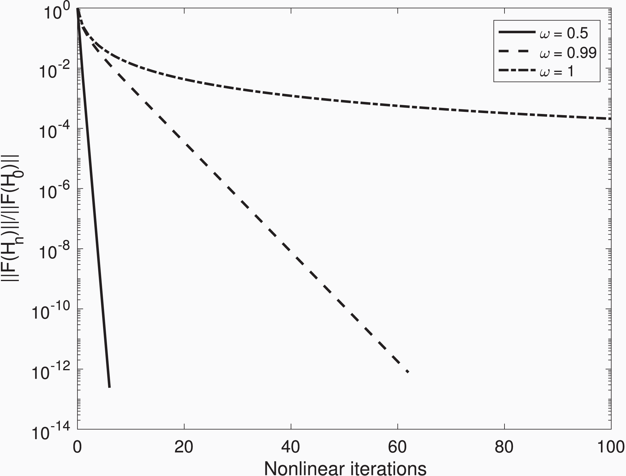
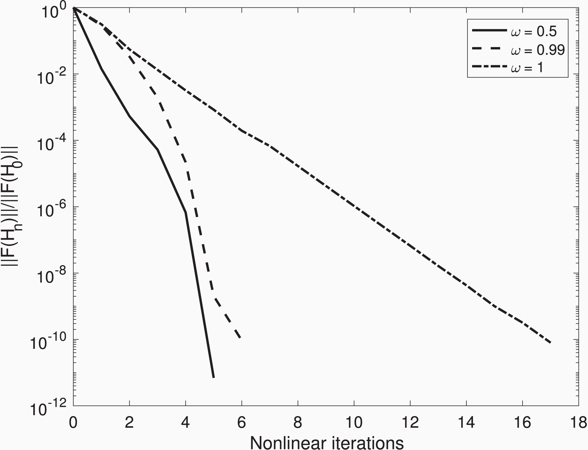
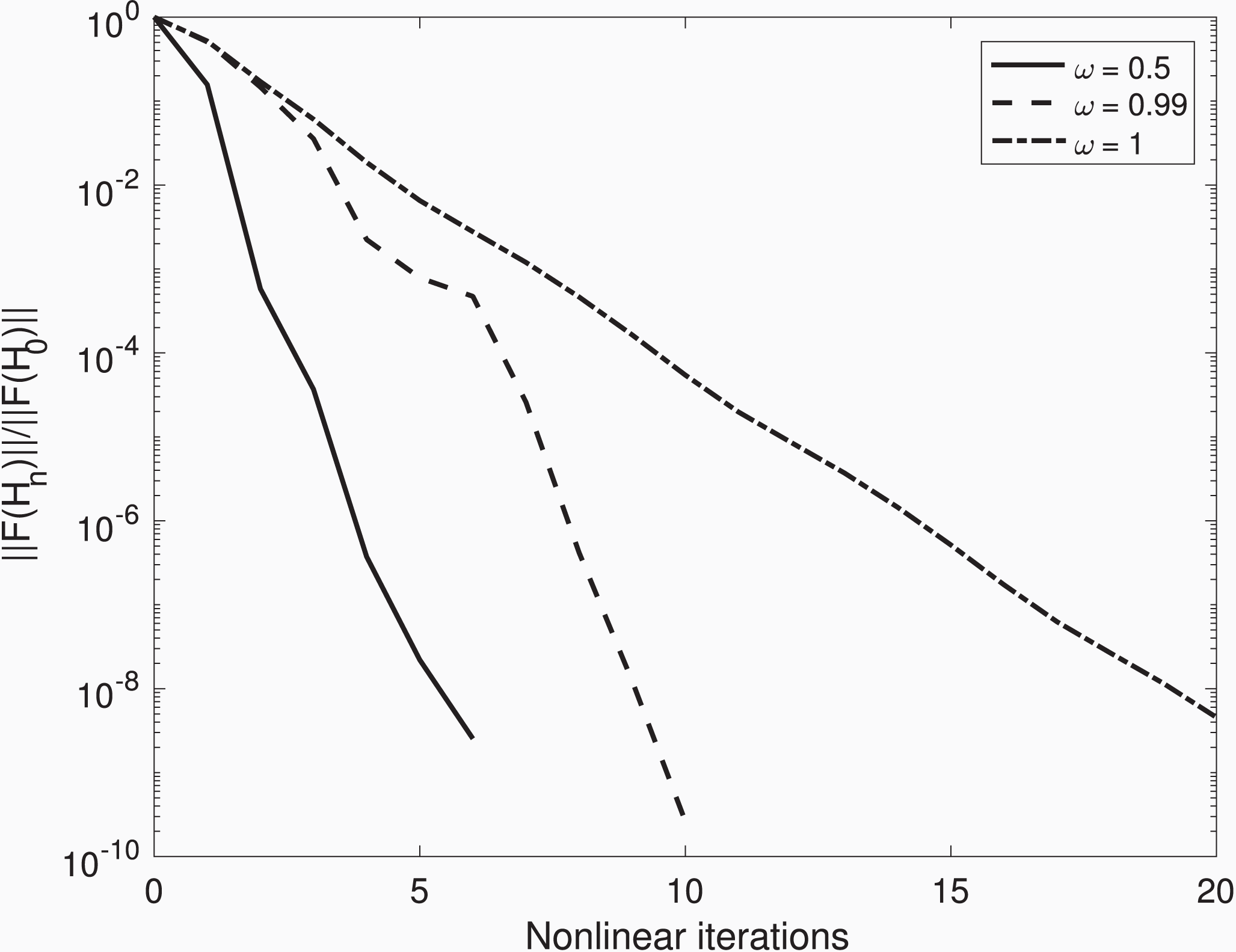
is large. In Figure 2.3 we plot the relative residual (
 $\Vert \mathbf{F}^{N}(\mathbf{h}_{n})\Vert /\Vert \mathbf{F}^{N}(\mathbf{h}_{0})\Vert$
) histories for the three values of
 $\unicode[STIX]{x1D714}$
.
Newton’s method for the
 $H$
-equation example.

The chord method for the
 $H$
-equation example.

Figure 2.3 reinforces the ideas from this section. The concave plots of residual histories for
 $\unicode[STIX]{x1D714}<1$
indicate superlinear convergence. The linear plot for
 $\unicode[STIX]{x1D714}=1$
, however, shows that the standard assumptions are violated in this case, as we demonstrated above. One can analyse this (Decker and Kelley Reference Decker and Kelley1980) and show that the simple scalar equation
 $x^{2}=0$
fully explains the q-/linear convergence rate. For any
 $x_{0}\neq 0$
, the Newton iteration for
 $x^{2}=0$
is simply
 $$\begin{eqnarray}x_{n}=x_{n-1}/2.\end{eqnarray}$$
Hence the convergence is q-linear with q-factor
 $1/2$
. The residuals
 $$\begin{eqnarray}x_{n}^{2}=x_{n-1}^{2}/4\end{eqnarray}$$
converge q-linearly to
 $0$
with q-factor
 $1/4$
.
In Figure 2.4 we plot the residual histories for the chord method. For
 $\unicode[STIX]{x1D714}=0.5$
and
 $\unicode[STIX]{x1D714}=0.99$
one can see the q-linear convergence predicted by theory. However, for
 $\unicode[STIX]{x1D714}=1$
something different is happening. The discussion for the continuous case applies without modification to the discrete problem and
 $\mathbf{F}^{\prime }(\mathbf{h}^{\ast })$
is singular for
 $\unicode[STIX]{x1D714}=1$
. There is theory for that case (Decker and Kelley Reference Decker and Kelley1983) and the results can be explained by considering the scalar equation
 $x^{2}=0$
. With the initial iterate
 $x_{0}=1$
the chord iterations are
 $$\begin{eqnarray}x_{n}=x_{n-1}(1-x_{n-1}/2)=O(1/n),\end{eqnarray}$$
which is very slow convergence.
If one refines the mesh for this problem, one will have a more accurate approximation of the solution of the integral equation. However, mesh refinement will have a very small effect on the iteration statistics. Table 2.3 illustrates this by showing some relative residual norms for the Newton iteration with
 $\unicode[STIX]{x1D714}=0.5$
and a few values of
 $N$
. As you can see, the relative residual norms are identical to three figures until the terminal iteration. This effect is called mesh independence. We will return to this topic in Section 3.3. We were limited to
 $N=8000$
because we could not store or factor larger dense matrices in our computing environment.
Newton residuals and timings.

We also report computer times in seconds using the MATLAB tic and toc commands. We do this only to show that the run times do not, as you might expect from the
 $O(N^{3})$
work in the matrix factorizations, increase by a factor of eight as we double the size of the problem. The reason for this is that there is a great deal of
 $O(N^{2})$
work in the Jacobian evaluations, which is significant in this case, and the LU factorization in MATLAB is very fast. The effects of the
 $O(N^{2})$
work are also seen in the chord iterations. One would expect the chord iterations to be much faster if the
 $O(N^{3})$
work in the matrix factorization dominated the computation. In Table 2.4 we show the first seven scaled residual norms for the chord iteration and the timings for the entire sequence of 63 iterations. As is the case with Newton’s method, the iteration statistics agree. Figures 2.3 and 2.4 would not change with higher values of
 $N$
.
Chord residuals and timings.

The performance of the JFNK iteration is far better because there is no
 $O(N^{2})$
work or storage at all – only the
 $O(N\log N)$
cost of the function evaluations. We will illustrate this by repeating the computations above with Newton–GMRES, a finite-difference Jacobian-vector product, and a constant forcing term of
 $\unicode[STIX]{x1D702}=0.1$
. The results were not affected by switching to an analytic Jacobian-vector product. In Figure 2.5 we plot the iteration histories. The curves are not as smooth as those in Figure 2.3, which reflects the limited accuracy of the linear solves. However, the overall cost was, as you will see in Table 2.5, much less.
Newton–GMRES for the
 $H$
-equation example.

The iteration is so fast that we must solve much larger problems to see the
 $O(N\log N)$
cost reflected in the timings. Table 2.5 shows the mesh independence of the nonlinear iteration. The performance of the linear iteration is also mesh-independent. For each value of
 $N$
the entire iteration needed
 $19$
calls to
 $\mathbf{F}^{N}$
. These
 $19$
calls include both the evaluation of the residual and the additional calls for the finite-difference Jacobian-vector product. One could also use an analytic Jacobian-vector product and both the cost and the results in Table 2.5 would be the same.
Newton–GMRES residuals and timings.

3 The Kantorovich theorem and mesh independence
The Kantorovich theorem is the nonlinear analogue of the ‘stability and consistency imply convergence’ results in differential equations (LeVeque Reference Leveque2007). The simplest example will illustrate the idea for linear problems. Suppose that
 $u^{\ast }$
is the solution of boundary value problem
 $$\begin{eqnarray}-u^{\prime \prime }(x)=f(x),u(0)=u(1)=0\end{eqnarray}$$
for some twice continuously differentiable function
 $f$
. Let
 $\mathbf{D}^{h}$
be the standard second-order approximation,
 $$\begin{eqnarray}\mathbf{D}^{h}=\displaystyle \frac{1}{h^{2}}\left(\begin{array}{@{}cccccc@{}}2 & -1 & 0 & \ldots \, & 0, & 0\\ -1 & 2 & -1 & ,0 & \ldots \, & 0\\ 0 & -1 & 2 & -1, & \ldots \, & 0\\ \vdots & \ddots & \ddots & \ddots & \ddots & \vdots \\ 0 & \ldots , & ,0, & -1 & 2 & -1\\ 0 & \ldots , & \ldots ,, & 0 & -1 & 2\\ \end{array}\right)\!,\end{eqnarray}$$
where
 $h=1/(N+1)$
is the spatial mesh width. Define
 ${\mathcal{E}}^{h}:C[0,1]\rightarrow \mathbb{R}^{N}$
by
 $$\begin{eqnarray}{\mathcal{E}}^{h}(u)_{i}=u(x_{i}),\end{eqnarray}$$
where
 $x_{i}=(i+1)h$
is the
 $i$
th interior grid point.
Second-order consistency is the statement that
 $$\begin{eqnarray}A^{h}{\mathcal{E}}u^{\ast }-{\mathcal{E}}f=O(h^{2}).\end{eqnarray}$$
Stability is the uniform boundedness of
 $\Vert (\mathbf{D}^{h})^{-1}\Vert$
, which is easy to verify. Together, stability and consistency imply that
 $$\begin{eqnarray}\Vert {\mathcal{E}}u^{\ast }-(\mathbf{D}^{h})^{-1}{\mathcal{E}}fl\Vert =O(h^{2})\end{eqnarray}$$
uniformly in
 $h$
. Hence, if
 $\mathbf{u}^{h}=(\mathbf{D}^{h})^{-1}{\mathcal{E}}f$
then
 $$\begin{eqnarray}\Vert \mathbf{u}^{h}-{\mathcal{E}}u^{\ast }\Vert =O(h^{2}),\end{eqnarray}$$
which is second-order convergence.
3.1 The theorem
The Kantorovich theorem (Kantorovich and Akilov Reference Kantorovich and Akilov1982) is a convergence result for Newton’s method that replaces the standard assumption that there is a solution with the statement that
 $\mathbf{F}(\mathbf{x}_{0})$
is sufficiently small (consistency). That coupled with a uniform bound on
 $\mathbf{F}^{\prime }(\mathbf{x})^{-1}$
in a neighbourhood of
 $\mathbf{x}_{0}$
(stability) implies that there is a unique solution
 $\mathbf{x}^{\ast }$
in a (smaller) neighbourhood of
 $\mathbf{x}_{0}$
and that
 $\mathbf{x}^{\ast }$
is near
 $\mathbf{x}_{0}$
(convergence!).
We use the formulation of the theorem from Ortega and Rheinboldt (Reference Ortega and Rheinboldt1970). There are several variations of the theorem. In addition to Ortega and Rheinboldt (Reference Ortega and Rheinboldt1970) and Kantorovich and Akilov (Reference Kantorovich and Akilov1982), one can find examples of alternative formulations in Kelley (Reference Kelley1995), Dennis (Reference Dennis1969), and Dennis (Reference Dennis and Rall1971). In Section 6.2 we will present a version from Qi and Sun (Reference Qi and Sun1993) for non-smooth functions.
The assumptions are similar to the standard assumptions.
Assumption 3.1.
 $\mathbf{F}$
is defined and Lipschitz continuously differentiable in
 ${\mathcal{D}}\subset \mathbb{R}^{N}$
.
∙ Equation (2.1) holds for all
$x,y\in {\mathcal{D}}$
.∙
$\Vert \mathbf{F}^{\prime }(\mathbf{x})^{-1}\Vert \leq \unicode[STIX]{x1D6FD}$
for all
$\mathbf{x}\in {\mathcal{D}}$
.∙ There is
$\mathbf{x}_{0}\in {\mathcal{D}}$
such that
$\Vert \mathbf{F}^{\prime }(\mathbf{x}_{0})^{-1}\mathbf{F}(\mathbf{x}_{0})\Vert \leq \unicode[STIX]{x1D702}$
.∙
$\unicode[STIX]{x1D6FC}\equiv \unicode[STIX]{x1D6FD}\unicode[STIX]{x1D6FE}\unicode[STIX]{x1D702}\leq 1/2$
.∙ The ball
${\mathcal{B}}(\mathbf{x}_{0},r_{+})\subset {\mathcal{D}}$
, where $$\begin{eqnarray}r_{\pm }=\displaystyle \frac{1\pm \sqrt{1-2\unicode[STIX]{x1D6FC}}}{\unicode[STIX]{x1D6FD}\unicode[STIX]{x1D6FE}}.\end{eqnarray}$$


Note that the assumptions on
 $\mathbf{x}_{0}$
cannot be stated in terms of
 $\Vert \mathbf{x}_{0}-\mathbf{x}^{\ast }\Vert$
because the existence of
 $\mathbf{x}^{\ast }$
is part of the conclusion of the theorem. Rather, one uses
 $\Vert \mathbf{F}^{\prime }(\mathbf{x}_{0})^{-1}\mathbf{F}(\mathbf{x}_{0})\Vert$
as a surrogate. However, the theorem will imply that
 $$\begin{eqnarray}\unicode[STIX]{x1D702}\geq \Vert \mathbf{F}^{\prime }(\mathbf{x}_{0})^{-1}\mathbf{F}(\mathbf{x}_{0})\Vert =\Vert \mathbf{e}_{0}\Vert +O(\Vert \mathbf{e}_{0}\Vert ^{2}).\end{eqnarray}$$
Since
 $\unicode[STIX]{x1D6FD}=\Vert \mathbf{F}^{\prime }(\mathbf{x}^{\ast })^{-1}\Vert +O(\Vert \mathbf{e}_{0}\Vert )$
, the assumption
 $\unicode[STIX]{x1D6FD}\unicode[STIX]{x1D6FE}\unicode[STIX]{x1D702}<1/2$
implies that
 $$\begin{eqnarray}\Vert \mathbf{e}_{0}\Vert \leq \displaystyle \frac{\Vert \mathbf{F}^{\prime }(\mathbf{x}^{\ast })^{-1}\Vert ^{-1}}{2\unicode[STIX]{x1D6FE}}+O(\Vert \mathbf{e}_{0}\Vert ^{2}),\end{eqnarray}$$
which is close to (2.3) if
 $\Vert \mathbf{e}_{0}\Vert$
is small enough to permit one to neglect the second-order term. One remarkable fact about the Kantorovich theorem is that there is no need for
 $\Vert \mathbf{e}_{0}\Vert$
to be small to obtain convergence. In that sense the theorem is a global convergence result. This is why one cannot expect q-quadratic convergence for the entire iteration. The r-quadratic convergence one obtains from the theorem is remarkable.
Theorem 3.2. Let Assumption 3.1 hold. Then there is a unique root
 $x^{\ast }$
of
 $F$
in
 ${\mathcal{B}}(\mathbf{x}_{0},r_{+})$
, the Newton iteration with
 $\mathbf{x}_{0}$
as the initial iterate converges to
 $\mathbf{x}^{\ast }$
, and
 $x_{n}\in {\mathcal{B}}(\mathbf{x}_{0},r_{-})$
for all
 $n$
. The errors satisfy the estimate
 $$\begin{eqnarray}\Vert \mathbf{e}_{n}\Vert \leq \displaystyle \frac{(2\unicode[STIX]{x1D6FD}\unicode[STIX]{x1D702}\unicode[STIX]{x1D6FE})^{2^{n}}}{2^{n}\unicode[STIX]{x1D6FD}\unicode[STIX]{x1D6FE}},\end{eqnarray}$$
and hence the convergence is r-quadratic.
We refer to Ortega and Rheinboldt (Reference Ortega and Rheinboldt1970) for the proof and to Kelley (Reference Kelley1995) for a simpler proof of an analogous theorem for the chord method. The proof in Kelley (Reference Kelley1995) is based on directly showing that the chord map
 $$\begin{eqnarray}\mathbf{G}_{C}(\mathbf{x})=\mathbf{x}-\mathbf{F}^{\prime }(\mathbf{x}_{0})^{-1}\mathbf{F}(\mathbf{x})\end{eqnarray}$$
is a contraction on
 ${\mathcal{B}}(\mathbf{x}_{0},r_{-})$
. The proof of Theorem 3.2 uses a recursion relation for a bound on the steps to show that the Newton map
 $$\begin{eqnarray}\mathbf{G}_{N}(\mathbf{x})=\mathbf{x}-\mathbf{F}^{\prime }(\mathbf{x})^{-1}\mathbf{F}(\mathbf{x})\end{eqnarray}$$
is a contraction and to obtain the convergence rate estimate (3.1).
3.2 A boundary value problem
In this section we will illustrate in some detail how the Kantorovich theorem can be applied to show convergence of a finite-difference approximation to a nonlinear two-point boundary value problem. We will begin with an existence/uniqueness result for the continuous problem and then directly estimate
 $\unicode[STIX]{x1D702}$
,
 $\unicode[STIX]{x1D6FD}$
and
 $\unicode[STIX]{x1D6FE}$
to apply the Kantorovich theorem.
The boundary problem is
 $$\begin{eqnarray}-u^{\prime \prime }(x)-\cos (u)=0,\quad u(0)=u(1)=0.\end{eqnarray}$$
We will use the contraction mapping theorem in the space
 $C[0,1]$
to prove existence and uniqueness of a solution of (3.2).
Let
 ${\mathcal{G}}$
be the inverse of the negative Laplacian in one space dimension with homogeneous Dirichlet boundary conditions, that is,
 $$\begin{eqnarray}{\mathcal{G}}(u)(x)=\int _{0}^{1}g(x,y)u(y)\,\text{d}y,\end{eqnarray}$$
where the Green’s function
 $g$
is
 $$\begin{eqnarray}g(x,z)=\left\{\begin{array}{@{}ll@{}}x(1-z)\quad & 0<x<z,\\ z(1-x)\quad & z<x<1.\end{array}\right.\end{eqnarray}$$
If
 $f\in C[0,1]$
and
 $u={\mathcal{G}}(f)$
, then
 $$\begin{eqnarray}-u^{\prime \prime }=f,\quad u(0)=u(1)=0.\end{eqnarray}$$
Hence (3.2) has a solution if and only if the equivalent integral equation
 $$\begin{eqnarray}{\mathcal{F}}(u)(x)=u(x)-\int _{0}^{1}g(x,y)\cos (u(y))\,\text{d}y=0\end{eqnarray}$$
has a solution. We express the integral equation as a fixed-point problem
 $$\begin{eqnarray}u(x)={\mathcal{K}}(u)(x)\equiv {\mathcal{G}}(\cos (u))(x),\end{eqnarray}$$
and will show that
 ${\mathcal{K}}$
is a contraction on
 $C[0,1]$
.
Clearly
 $$\begin{eqnarray}|\text{cos}(u)-\cos (v)|\leq |u-v|,\quad \text{for all }u,v.\end{eqnarray}$$
So
 $$\begin{eqnarray}|{\mathcal{K}}(u)(x)-{\mathcal{K}}(v)(x)|\leq \Vert u-v\Vert _{\infty }\int _{0}^{1}g(x,y)\,\text{d}y.\end{eqnarray}$$
Note that
 $$\begin{eqnarray}w(x)=\int _{0}^{1}g(x,y)\,\text{d}y=\displaystyle \frac{x(1-x)}{2}\end{eqnarray}$$
and hence
 $\Vert w\Vert _{\infty }=1/8$
. Thus
 $$\begin{eqnarray}\Vert {\mathcal{K}}(u)-{\mathcal{K}}(v)\Vert _{\infty }\leq \Vert u-v\Vert _{\infty }/8.\end{eqnarray}$$
So
 ${\mathcal{K}}$
is a contraction on
 $C[0,1]$
. We now know that the boundary value problem has a unique solution
 $u^{\ast }\in C[0,1]$
. We have also derived a uniform bound for
 ${\mathcal{F}}^{\prime }(u)^{-1}$
. For any
 $w\in C[0,1]$
we have (using (2.27))
 $$\begin{eqnarray}{\mathcal{F}}^{\prime }(u)w(x)=w(x)+\int _{0}^{1}g(x,y)\sin (u(y))w(y)\,\text{d}y\end{eqnarray}$$
and so
 $$\begin{eqnarray}\Vert {\mathcal{F}}^{\prime }(u)w\Vert _{\infty }\geq (7/8)\Vert w\Vert _{\infty }.\end{eqnarray}$$
Hence
 $$\begin{eqnarray}\Vert {\mathcal{F}}^{\prime }(u)^{-1}\Vert _{\infty }\leq 8/7\end{eqnarray}$$
for all
 $u\in C[0,1]$
. We can also conclude from the above that
 ${\mathcal{F}}^{\prime }$
is Lipschitz continuous with Lipschitz constant
 $\unicode[STIX]{x1D6FE}\leq 1/8$
.
We discretize the problem with central finite differences with a uniform mesh width
 $h$
. The discrete problem is
 $$\begin{eqnarray}\mathbf{D}^{h}\mathbf{u}^{h}+\cos (\mathbf{u}^{h})=0.\end{eqnarray}$$
We precondition with
 $\mathbf{G}^{h}\equiv (\mathbf{D}^{h})^{-1}$
and obtain the analogue of (3.4):
 $$\begin{eqnarray}\mathbf{F}^{h}(\mathbf{u}^{h})=\mathbf{u}^{h}+\mathbf{G}^{h}\cos (\mathbf{u}^{h})\equiv \mathbf{u}^{h}+\mathbf{K}^{h}(\mathbf{u}^{h}).\end{eqnarray}$$
The smoothness of
 $u^{\ast }$
implies that there is
 $\unicode[STIX]{x1D702}_{0}>0$
such that
 $$\begin{eqnarray}\Vert \mathbf{F}^{h}({\mathcal{E}}^{h}u^{\ast })\Vert _{\infty }\leq \unicode[STIX]{x1D702}_{0}h^{2}\end{eqnarray}$$
and that
 $$\begin{eqnarray}\Vert (\mathbf{F}^{h})^{-1}(u)\Vert _{\infty }\leq 2\end{eqnarray}$$
uniformly in
 $u$
and
 $h$
. Clearly the Lipschitz constant
 $\unicode[STIX]{x1D6FE}^{h}$
of of
 $(\mathbf{F}^{h})^{\prime }$
is
 $\leq 1/4$
for
 $h$
sufficiently small.
We are can now apply the Kantorovich theorem to show that a solution
 $\mathbf{u}^{h}$
of (3.5) exists and that
 $$\begin{eqnarray}\Vert \mathbf{u}^{h}-{\mathcal{E}}^{h}u^{\ast }\Vert _{\infty }=O(h^{2}).\end{eqnarray}$$
We will apply the theorem with
 $\unicode[STIX]{x1D6FD}=2$
from (3.7),
 $\unicode[STIX]{x1D702}=2\unicode[STIX]{x1D702}_{0}h^{2}$
from (3.6) and (3.7), and
 $\unicode[STIX]{x1D6FE}=\unicode[STIX]{x1D6FE}^{h}=1/4$
. Then
 $$\begin{eqnarray}\unicode[STIX]{x1D6FC}=\unicode[STIX]{x1D702}_{0}h^{2}<1/2\end{eqnarray}$$
for
 $h$
sufficiently small. So there is a solution
 $\mathbf{u}^{h}$
in
 ${\mathcal{B}}({\mathcal{E}}^{h}u^{\ast },r_{-})$
where
 $$\begin{eqnarray}r_{-}=\displaystyle \frac{1-\sqrt{1-2\unicode[STIX]{x1D6FC}}}{\unicode[STIX]{x1D6FD}\unicode[STIX]{x1D6FE}}=\displaystyle \frac{1-\sqrt{1-2\unicode[STIX]{x1D702}_{0}h^{2}}}{1/2}=O(h^{2}).\end{eqnarray}$$
Summarizing, stability (3.7) and consistency (3.6) imply convergence.
3.3 Mesh independence results
The example in Section 3.2 made use of the fact that the parameters in the Kantorovich theorem could be estimated independently of the mesh
 $h$
. Hence the convergence estimate in (3.1) is also independent of
 $h$
. This is a simple example of a mesh independence theorem. In this section we will explore two variations of this idea. Classical mesh independence results are about the convergence of the iteration statistics to those of an underlying infinite-dimensional problem as a grid is refined. In this case the errors are deterministic and we look at some of the ideas in this section. After that we consider tracking theorems. These results describe convergence of the iteration statistics when the errors are stochastic and depend, for example, on the sample size.
3.3.1 Deterministic errors
The concept of mesh independence has its origin in Allgower, Böhmer, Potra and Rheinboldt (Reference Allgower, Böhmer, Potra and Rheinboldt1986). While the results may seem obvious, mesh independence is a very useful concept in both nonlinear equations (Kelley and Sachs Reference Kelley and Sachs1991, Ferng and Kelley Reference Ferng and Kelley2000) and optimization (Sachs Reference Sachs1990, Hintermüller and Ulbrich Reference Hintermüller and Ulbrich2003).
The idea is that one is approximating an infinite-dimensional equation
 $$\begin{eqnarray}{\mathcal{F}}(u)=0,\end{eqnarray}$$
defined on a Banach space
 $X$
, with a sequence of finite-dimensional problems
 $$\begin{eqnarray}\mathbf{F}^{h}(\mathbf{u})=0\end{eqnarray}$$
on
 $\mathbb{R}^{N}$
. The boundary value problem from Section 3.2 and the Chandrasekhar
 $H$
-equation from Section 2.10 are examples of this situation. We will be interested in a solution
 $u^{\ast }$
of (3.9) at which the standard assumptions hold.
In both of these examples the performance of Newton’s method is mesh-independent in the sense that the relative residuals not only converge to zero, but also converge for each iteration as the mesh is refined. In Section 3.2 we introduced one way to quantify this. Let
 ${\mathcal{E}}^{h}:X\rightarrow \mathbb{R}^{N}$
be the projection from the space
 $X$
to
 $\mathbb{R}^{N}$
that encodes the discretization. For a finite-difference approximation, for example,
 ${\mathcal{E}}^{h}$
could be evaluation at the grid points.
Convergence of the approximation means that the solution
 $\mathbf{u}^{h}$
of (3.10) satisfies
 $$\begin{eqnarray}\lim _{h\rightarrow 0}\Vert \mathbf{u}^{h}-{\mathcal{E}}^{h}u^{\ast }\Vert =0.\end{eqnarray}$$
In many cases, including the examples in Sections 3.2 and 2.10, one can show that the Newton iterations also converge in the sense that
 $$\begin{eqnarray}\lim _{h\rightarrow 0}\Vert \mathbf{u}_{n}^{h}-{\mathcal{E}}^{h}u_{n}\Vert =0,\end{eqnarray}$$
where
 $\mathbf{u}_{n}^{h}$
is the
 $n$
th Newton iteration for (3.10) and
 $u_{n}$
is the
 $n$
th Newton iteration for (3.9).
We will express the fact that the iteration statistics converge in two ways, both of which follow from (3.11) and (3.12). These results also hold for the JFNK methods we discussed in Section 2.6. We will denote the infinite-dimensional iteration
 $$\begin{eqnarray}u_{n+1}=u_{n}-{\mathcal{F}}^{\prime }(u_{n})^{-1}{\mathcal{F}}(u_{n}).\end{eqnarray}$$
∙ Let
$\unicode[STIX]{x1D716}>0$
and let
$k^{h}$
be the least
$k$
such that
$\Vert \mathbf{F}^{h}(\mathbf{u}_{k}^{h})\Vert /\Vert \mathbf{F}^{h}(\mathbf{u}_{0}^{h})\Vert <\unicode[STIX]{x1D716}$
. Let
$k^{0}$
be the least
$k$
such that Then, for all$$\begin{eqnarray}\Vert {\mathcal{F}}(u_{k})\Vert /\Vert {\mathcal{F}}(u_{0})\Vert <\unicode[STIX]{x1D716}.\end{eqnarray}$$
$h$
sufficiently small,
$|k^{h}-k^{0}|\leq 1$
.∙ Let
$K>0$
and let
$\unicode[STIX]{x1D716}>0$
be given. Then, for
$h$
sufficiently small, for all$$\begin{eqnarray}\biggl|\displaystyle \frac{\Vert \mathbf{F}^{h}(\mathbf{u}_{k}^{h})\Vert }{\Vert \mathbf{F}^{h}(\mathbf{u}_{0}^{h})\Vert }-\displaystyle \frac{\Vert {\mathcal{F}}(u_{k}^{h})\Vert }{\Vert {\mathcal{F}}(u_{0})\Vert }\biggr|<\unicode[STIX]{x1D716}\end{eqnarray}$$
$0\leq k\leq K$
.


3.3.2 Tracking theorems
The results in Willert, Chen and Kelley (Reference Willert, Chen and Kelley2015) consider the case where the function
 $\mathbf{F}$
, the Jacobian
 $\mathbf{F}^{\prime }$
and Jacobian-vector products are not evaluated directly, but are approximated using internal Monte Carlo computations. The work was motivated by problems in neutron transport (Willert, Kelley, Knoll and Park Reference Willert, Kelley, Knoll and Park2013, Knoll, Park and Smith Reference Knoll, Park and Smith2011), where a Monte Carlo simulation was embedded in the residual. The results are similar to mesh independence theorems in that one seeks to show that some finite subset of the iterations converges, but does not seek to drive the approximation error (or its variance) to zero. However, the assumptions and convergence theorems are more technical. We used the term ‘tracking’ in Willert et al. (Reference Willert, Chen and Kelley2015) rather than convergence.
We approximate functions, Jacobians, and Jacobian-vector projects with a Monte Carlo simulation with a sample size
 $N_{\text{MC}}$
. The notation from Willert et al. (Reference Willert, Chen and Kelley2015) is as follows.
∙
$N_{\text{MC}}$
is the sample size for the function and
$N_{\text{MC}}^{J}$
is the sample size for the Jacobian or Jacobian-vector product.∙
$\tilde{\mathbf{F}}(\mathbf{x},N_{\text{MC}})$
is an outcome of the simulation for the residual
$\mathbf{F}(\mathbf{x})$
.∙
$\mathbf{J}(\mathbf{x},N_{\text{MC}}^{J})$
is an outcome of the simulation for the Jacobian
$\mathbf{F}^{\prime }(\mathbf{x})$
.∙
$\mathbf{J}_{p}(\mathbf{x},\mathbf{v},N_{\text{MC}}^{J})$
is an outcome of the simulation for the Jacobian-vector product
$\mathbf{F}^{\prime }(\mathbf{x})\mathbf{v}$
.


We assume that the evaluations of
 $\tilde{\mathbf{F}}$
,
 $\mathbf{J}$
and
 $\mathbf{J}_{p}$
are independent.
Suppose the standard assumptions hold and that Newton’s method converges for all
 $\mathbf{u}\in {\mathcal{B}}(\mathbf{x}^{\ast },\unicode[STIX]{x1D70C})$
. We make a consistency assumption for the function and Jacobian evaluations.
Assumption 3.3. There are functions
 $c_{F}$
,
 $c_{J}$
and
 $c_{Jv}$
and an open set
 ${\mathcal{B}}^{\prime }$
which contains
 ${\mathcal{B}}(\mathbf{x}^{\ast },\unicode[STIX]{x1D70C})$
such that, for all
 $\mathbf{x}\in {\mathcal{B}}^{\prime }$
, unit vectors
 $\mathbf{v}\in \mathbb{R}^{N}$
and
 $\unicode[STIX]{x1D6FF}>0$
,
 $$\begin{eqnarray}\displaystyle \operatorname{Prob}\biggl(\Vert \mathbf{F}(\mathbf{x})-\tilde{\mathbf{F}}(\mathbf{x},N_{\text{MC}})\Vert >\displaystyle \frac{c_{F}(\unicode[STIX]{x1D6FF})}{\sqrt{N_{\text{MC}}}}\biggr) & {<} & \displaystyle \unicode[STIX]{x1D6FF},\end{eqnarray}$$
 $$\begin{eqnarray}\displaystyle \operatorname{Prob}\biggl(\Vert \mathbf{F}^{\prime }(\mathbf{x})-\mathbf{J}(\mathbf{x},N_{\text{MC}}^{J})\Vert >\displaystyle \frac{c_{J}(\unicode[STIX]{x1D6FF})}{\sqrt{N_{\text{MC}}^{J}}}\biggr) & {<} & \displaystyle \unicode[STIX]{x1D6FF}.\end{eqnarray}$$
In this article we will only summarize the results from Willert et al. (Reference Willert, Chen and Kelley2015) on methods which use full Jacobians. The assumptions on the quality of the residual evaluation and the Jacobian are not sufficient to guarantee quadratic convergence. The algorithm increases the number of samples as the iteration progresses, which sometimes reflects practice. One would never increase the number of samples rapidly enough to capture superlinear convergence, and the theory reflects that. The algorithm from Willert et al. (Reference Willert, Chen and Kelley2015) is given in algorithm newton_MC.

Theorem 3.4. Let (3.13) and (3.14) from Assumption 3.3 and the assumptions of Theorem 2.2 hold. Let
 $r_{\text{Newton}}\in (0,1)$
be given and assume that
 $\Vert \mathbf{e}_{0}\Vert \leq \unicode[STIX]{x1D70C}$
and
 $\hat{\unicode[STIX]{x1D702}}$
are small enough for the inexact Newton iteration to converge q-linearly with a q-factor
 $r_{\text{Newton}}$
. Let a positive integer
 $K$
,
 $r\in (r_{\text{Newton}},1)$
and
 $\unicode[STIX]{x1D714}\in (0,1)$
be given. Then there are
 $\hat{\unicode[STIX]{x1D702}}$
,
 $N_{\text{MC}}$
,
 $N_{\text{MC}}^{J}$
and
 $N_{\text{inc}}$
, such that, with probability
 $(1-\unicode[STIX]{x1D714})$
for all
 $1\leq n\leq K$
, the iteration produced by algorithm newton_MC satisfies
 $$\begin{eqnarray}\Vert \mathbf{e}_{n}\Vert \leq r^{n}\Vert \mathbf{e}_{0}\Vert ,\end{eqnarray}$$
If one approximates matrix–vector products rather than the Jacobian itself, then assumption (3.14) must be replaced by one on the matrix–vector product computation. The subtle, and important, problem with this is that there is no underlying matrix. This can (and does: see Willert et al. Reference Willert, Kelley, Knoll and Park2013) produce error accumulation in the Krylov method. Simoncini and Szyld (Reference Simoncini and Szyld2003a , Reference Simoncini and Szyld2003b , Reference Simoncini and Szyld2007) explain this in detail. Willert et al. (Reference Willert, Chen and Kelley2015) use that analysis to derive very technical tracking results, which we mercifully omit from this paper, for matrix-free methods.
4 Pseudo-arclength continuation
This section is the first of three (see also Sections 6.4 and 7) on continuation methods. In this section we will look at parameter-dependent nonlinear equations
 $$\begin{eqnarray}\mathbf{F}(\mathbf{x},\unicode[STIX]{x1D706})=0\end{eqnarray}$$
and the dependence of the solution(s) on the parameter
 $\unicode[STIX]{x1D706}$
. The parameter
 $\unicode[STIX]{x1D714}$
in the
 $H$
-equation is one example. Other examples are the load in a mechanics problem or the voltage in circuit design. In general
 $\unicode[STIX]{x1D706}$
can be a vector, but we will only consider scalars in this section.
The study of parameter-dependent systems is deeply connected to dynamics (Govaerts Reference Govaerts2000, Keller Reference Keller1987, Marsden and McCracken Reference Marsden and McCracken1976, Kuznetsov Reference Kuznetsov1998), but we will only examine that connection in a superficial way in Section 7. In particular we will not cover bifurcation, the case where two different solution paths intersect. One must use the higher derivative tensors to understand singularities of that type.
One may think that this is a trivial problem. One could begin with
 $\unicode[STIX]{x1D706}_{0}$
and solve (4.1) for
 $\unicode[STIX]{x1D706}=\unicode[STIX]{x1D706}_{0}$
with the Armijo line search from Section 2.7 to find
 $\mathbf{x}^{\ast }(\unicode[STIX]{x1D706}_{0})$
. Then one picks an increment
 $\unicode[STIX]{x1D6FF}_{\unicode[STIX]{x1D706}}$
in the parameter and solves (4.1) for
 $\mathbf{x}(\unicode[STIX]{x1D706}+\unicode[STIX]{x1D6FF}_{\unicode[STIX]{x1D706}})$
with
 $\mathbf{x}^{\ast }(\unicode[STIX]{x1D706})$
as the initial iterate. Algorithm simple_continuation is a formal description of this simple parameter continuation idea.

Algorithm simple_continuation can only succeed if the range of
 $\unicode[STIX]{x1D706}$
is infinite. In the case of the
 $H$
-equation, for example, there are no real solutions for
 $\unicode[STIX]{x1D714}>1$
, and something must go wrong when
 $\unicode[STIX]{x1D714}=1$
and the Jacobian is singular at the solution. We explain that in the next section and then describe one possibility for resolving the problem.
4.1 The implicit function theorem
The implicit function theorem says that algorithm simple_continuation will successfully follow the solution path as long as
 $\mathbf{F}^{\prime }$
is safely non-singular and also provides an estimate of
 $\unicode[STIX]{x1D6FF}_{\unicode[STIX]{x1D706}}$
. We give a proof that is a nice application of the Kantorovich theorem.
We begin with some notation. If
 $\mathbf{F}(\mathbf{x},\unicode[STIX]{x1D706})$
is a function of
 $\mathbf{x}\in \mathbb{R}^{N}$
and
 $\unicode[STIX]{x1D706}\in R$
, then
 $\mathbf{F}_{\mathbf{x}}$
will denote the Jacobian in the
 $\mathbf{x}$
variable. Hence
 $\mathbf{F}_{\mathbf{x}}$
is an
 $N\times N$
matrix. Similarly
 $\mathbf{F}_{\unicode[STIX]{x1D706}}\in \mathbb{R}^{N}$
is the partial of
 $\mathbf{F}$
with respect to the scalar variable
 $\unicode[STIX]{x1D706}$
.
Theorem 4.1. Assume the following:
∙
$\mathbf{F}(\mathbf{x}_{0},\unicode[STIX]{x1D706}_{0})=0$
;∙
$\mathbf{F}$
is a continuously differentiable function of
$\unicode[STIX]{x1D706}$
;∙
$\mathbf{F}_{\mathbf{x}}$
and
$\mathbf{F}$
are Lipschitz continuous in
$(\mathbf{x},\unicode[STIX]{x1D706})$
with Lipschitz constant
$\unicode[STIX]{x1D6FE}$
, that is, and$$\begin{eqnarray}\Vert \mathbf{F}(\mathbf{x},\unicode[STIX]{x1D706})-\mathbf{F}(\mathbf{y},\unicode[STIX]{x1D707})\Vert \leq \unicode[STIX]{x1D6FE}(\Vert \mathbf{x}-\mathbf{y}\Vert +|\unicode[STIX]{x1D706}-\unicode[STIX]{x1D707}|)\end{eqnarray}$$
$$\begin{eqnarray}\Vert \mathbf{F}_{\mathbf{x}}(\mathbf{x},\unicode[STIX]{x1D706})-\mathbf{F}_{\mathbf{x}}(\mathbf{y},\unicode[STIX]{x1D707})\Vert \leq \unicode[STIX]{x1D6FE}(\Vert \mathbf{x}-\mathbf{y}\Vert +|\unicode[STIX]{x1D706}-\unicode[STIX]{x1D707}|);\end{eqnarray}$$
∙
$\mathbf{F}_{\mathbf{x}}(\mathbf{x}_{0},\unicode[STIX]{x1D706}_{0})$
is non-singular and
$\Vert \mathbf{F}_{\mathbf{x}}^{-1}(\mathbf{x}_{0},\unicode[STIX]{x1D706}_{0})\Vert \leq \unicode[STIX]{x1D6FD}_{0}$
.


Then there are
 $\unicode[STIX]{x1D6E5}$
and
 $r$
, which depend only on
 $\unicode[STIX]{x1D6FD}$
and
 $\unicode[STIX]{x1D6FE}$
, such that the following hold:
∙ there is a solution
$\mathbf{x}(\unicode[STIX]{x1D706})$
of (4.1) for all
$\unicode[STIX]{x1D706}$
such that
$|\unicode[STIX]{x1D706}-\unicode[STIX]{x1D706}_{0}|\leq \unicode[STIX]{x1D6E5}$
;∙
$\mathbf{x}(\unicode[STIX]{x1D706}_{0})=\mathbf{x}_{0}$
;∙
$\mathbf{x}(\unicode[STIX]{x1D706})$
is the only solution of (4.1) for
$\Vert \mathbf{x}-\mathbf{x}_{0}\Vert \leq r$
;∙
$\mathbf{x}(\unicode[STIX]{x1D706})$
is a continuously differentiable function of
$\unicode[STIX]{x1D706}$
.


Proof. Similarly to the proof of Theorem 2.2, Lipschitz continuity of
 $\mathbf{F}_{\mathbf{x}}$
implies that
 $\mathbf{F}_{\mathbf{x}}(\mathbf{x},\unicode[STIX]{x1D706})$
is non-singular in the set
 $$\begin{eqnarray}{\mathcal{D}}=\biggl\{(\mathbf{x},\unicode[STIX]{x1D706})\mid \Vert \mathbf{x}-\mathbf{x}_{0}\Vert +|\unicode[STIX]{x1D706}-\unicode[STIX]{x1D706}_{0}|\leq \displaystyle \frac{1}{2\unicode[STIX]{x1D6FE}\Vert \mathbf{F}_{\mathbf{x}}^{-1}(\mathbf{x}_{0},\unicode[STIX]{x1D706}_{0})\Vert }\biggr\},\end{eqnarray}$$
and that
 $$\begin{eqnarray}\Vert \mathbf{F}_{\mathbf{x}}^{-1}(\mathbf{x},\unicode[STIX]{x1D706})\Vert \leq \unicode[STIX]{x1D6FD}\equiv 2\unicode[STIX]{x1D6FD}_{0}\end{eqnarray}$$
for all
 $(\mathbf{x},\unicode[STIX]{x1D706})\in {\mathcal{D}}$
.
We have
 $\unicode[STIX]{x1D6FD}$
and
 $\unicode[STIX]{x1D6FE}$
in hand for an application of the Kantorovich theorem. We use Lipschitz continuity of
 $\mathbf{F}$
to obtain
 $$\begin{eqnarray}\Vert \mathbf{F}(\mathbf{x}_{0},\unicode[STIX]{x1D706})\Vert =\Vert \mathbf{F}(\mathbf{x}_{0},\unicode[STIX]{x1D706})-\mathbf{F}(\mathbf{x}_{0},\unicode[STIX]{x1D706}_{0})\Vert \leq \unicode[STIX]{x1D6FE}|\unicode[STIX]{x1D706}-\unicode[STIX]{x1D706}_{0}|\equiv \unicode[STIX]{x1D702}.\end{eqnarray}$$
So if
 $\unicode[STIX]{x1D6FE}^{2}\unicode[STIX]{x1D6FD}\unicode[STIX]{x1D6E5}<1/2$
and
 $|\unicode[STIX]{x1D706}-\unicode[STIX]{x1D706}_{0}|\leq \unicode[STIX]{x1D6E5}$
, we can apply the Kantorovich theorem with
 $$\begin{eqnarray}\unicode[STIX]{x1D6FC}=\unicode[STIX]{x1D6FD}\unicode[STIX]{x1D6FE}\unicode[STIX]{x1D702}=\unicode[STIX]{x1D6FD}\unicode[STIX]{x1D6FE}^{2}\unicode[STIX]{x1D6E5}\leq 1/2,\end{eqnarray}$$
to complete the proof of existence with
 $$\begin{eqnarray}r=\displaystyle \frac{1\pm \sqrt{1+2\unicode[STIX]{x1D6FC}}}{\unicode[STIX]{x1D6FD}\unicode[STIX]{x1D6FE}}.\end{eqnarray}$$
To show differentiability, we formally differentiate (4.1) with respect to
 $\unicode[STIX]{x1D706}$
and note that
 $\mathbf{x}^{\prime }(\unicode[STIX]{x1D706})$
is the solution
 $\mathbf{z}$
of

If
 $\mathbf{F}$
has higher-order derivatives, one can show that
 $\mathbf{x}$
has as many derivatives in
 $\unicode[STIX]{x1D706}$
as
 $\mathbf{F}$
does in
 $(\mathbf{x},\unicode[STIX]{x1D706})$
(Rabinowitz Reference Rabinowitz1971).
If
 $\mathbf{F}_{\mathbf{x}}(\mathbf{x}^{\ast },\unicode[STIX]{x1D706}^{\ast })$
is singular, then the implicit function cannot be used to assert that there are solutions near
 $\unicode[STIX]{x1D706}^{\ast }$
. In the case of the
 $H$
-equation,
 $\mathbf{F}_{\mathbf{h}}(\mathbf{h}^{\ast },1)$
is singular and (2.34) implies that there is no real solution for
 $\unicode[STIX]{x1D714}>1$
.
So, does the solution arc stop dead at the point
 $(H(1),1)$
? The answer is that for many common singularities, including the one for the
 $H$
-equation, the solution arc does not terminate abruptly but either loops back or becomes unbounded (Crandall and Rabinowitz Reference Crandall and Rabinowitz1971, Rabinowitz Reference Rabinowitz1971, Keller Reference Keller1987). We will discuss some specific examples in the rest of this section.
4.2 Simple folds and pseudo-arclength continuation
We will begin this section with an example that is both simple and general. Consider the scalar equation
 $$\begin{eqnarray}f(x,\unicode[STIX]{x1D706})=x^{2}-\unicode[STIX]{x1D706}.\end{eqnarray}$$
The function
 $f$
is Lipschitz continuous if
 $x$
is restricted to a bounded set. Since
 $f_{x}=2x$
the Lipschitz constant of the derivative is
 $2$
. There is a unique solution
 $x(0)=0$
when
 $\unicode[STIX]{x1D706}=0$
, no real solution when
 $\unicode[STIX]{x1D706}<0$
, and two solutions when
 $\unicode[STIX]{x1D706}>0$
. The singularity of
 $f_{x}$
at
 $\unicode[STIX]{x1D706}=0$
has, as we will see, exactly the same structure as the singularity of the
 $H$
-equation when
 $\unicode[STIX]{x1D714}=1$
.
Suppose we begin with
 $(x,\unicode[STIX]{x1D706})=(1,1)$
and try to use simple continuation to reach and pass
 $\unicode[STIX]{x1D706}=0$
. The continuation will fail because there is no solution for
 $\unicode[STIX]{x1D706}<0$
. However, the path of solutions continues beyond
 $\unicode[STIX]{x1D706}=0$
, the only difference being that the sign of
 $x$
changes. How can we modify the simple continuation algorithm to follow the path without getting stuck at the singularity?
One way would be to interchange the roles of
 $\unicode[STIX]{x1D706}$
and
 $x$
. This is the idea of the PITCON (Rheinboldt Reference Rheinboldt1986) code. If we do that, then
 $f_{\unicode[STIX]{x1D706}}=-1$
is never singular and we can continue with ease. The problem with this approach is that one must identify the variable to exchange with
 $\unicode[STIX]{x1D706}$
. Rheinboldt (Reference Rheinboldt1986) identifies many situations where this is readily done. There are many advanced continuation codes (Salinger et al.
Reference Salinger, Bou-Rabee, Pawlowski, Wilkes, Burroughs, Lehoucq and Romero2002, Doedel and Kernévez Reference Doedel and Kernévez1986, Govaerts Reference Govaerts2000) and some very good books (Govaerts Reference Govaerts2000, Kuznetsov Reference Kuznetsov1998, Doedel Reference Doedel1997, Keller Reference Keller1987, Rheinboldt Reference Rheinboldt1986) on the topic.
The approach we describe in this section, pseudo-arclength continuation, attempts to parametrize the solution arc and then add an approximation to arclength as a new parameter (Keller Reference Keller1987).
To see how this would work, suppose that
 $x(s)$
and
 $\unicode[STIX]{x1D706}(s)$
are functions of an arclength parameter
 $s$
. Setting
 ${\dot{x}}=\text{d}x/\text{d}s$
and
 $\dot{\unicode[STIX]{x1D706}}=\text{d}\unicode[STIX]{x1D706}/\text{d}s$
, we use the arclength normalization
 $$\begin{eqnarray}{\dot{x}}^{2}+\dot{\unicode[STIX]{x1D706}}^{2}=1.\end{eqnarray}$$
We define an expanded equation in
 $\mathbf{z}=(x,\unicode[STIX]{x1D706})^{T}$
with
 $s$
as the parameter:
 $$\begin{eqnarray}\mathbf{G}(\mathbf{z},s)\equiv \left(\begin{array}{@{}c@{}}f(x,\unicode[STIX]{x1D706})\\ {\dot{x}}^{2}+\dot{\unicode[STIX]{x1D706}}^{2}-1\end{array}\right)=\left(\begin{array}{@{}c@{}}0\\ 0\end{array}\right)\!.\end{eqnarray}$$
If
 $\mathbf{g}_{\mathbf{z}}$
is non-singular and one can effectively approximate
 ${\dot{x}}$
and
 $\dot{\unicode[STIX]{x1D706}}$
, then one can apply simple continuation to the expanded system.
We will investigate the non-singularity of
 $\mathbf{G}_{\mathbf{z}}$
first. Clearly
 $$\begin{eqnarray}\mathbf{G}_{\mathbf{z}}=\left(\begin{array}{@{}cc@{}}f_{x} & f_{\unicode[STIX]{x1D706}}\\ {\dot{x}} & \dot{\unicode[STIX]{x1D706}}\end{array}\right)=\left(\begin{array}{@{}cc@{}}2x & -1\\ {\dot{x}} & \dot{\unicode[STIX]{x1D706}}\end{array}\right)\!,\end{eqnarray}$$
so
 $$\begin{eqnarray}\det (\mathbf{G}_{\mathbf{z}})=2x\dot{\unicode[STIX]{x1D706}}+{\dot{x}}.\end{eqnarray}$$
Use
 $f(x,\unicode[STIX]{x1D706})=0$
to get
 $$\begin{eqnarray}0=\,\text{d}f(x,\unicode[STIX]{x1D706})/\,\text{d}s=f_{x}{\dot{x}}+f_{\unicode[STIX]{x1D706}}\dot{\unicode[STIX]{x1D706}}=2x{\dot{x}}-\dot{\unicode[STIX]{x1D706}}\end{eqnarray}$$
and so
 $2x{\dot{x}}=\dot{\unicode[STIX]{x1D706}}$
Now multiply
 $\det (\mathbf{G}_{\mathbf{z}})=2x\dot{\unicode[STIX]{x1D706}}+{\dot{x}}$
by
 ${\dot{x}}$
and
 $$\begin{eqnarray}{\dot{x}}\det (\mathbf{G}_{\mathbf{z}})=2x{\dot{x}}\dot{\unicode[STIX]{x1D706}}+{\dot{x}}^{2}.\end{eqnarray}$$
Use
 $2x{\dot{x}}=\dot{\unicode[STIX]{x1D706}}$
and
 $$\begin{eqnarray}{\dot{x}}\det (\mathbf{G}_{\mathbf{z}})=\dot{\unicode[STIX]{x1D706}}^{2}+{\dot{x}}^{2}=1.\end{eqnarray}$$
So
 $\det (\mathbf{G}_{\mathbf{z}})\neq 0$
.
One way to approximate
 ${\dot{x}}$
and
 $\dot{\unicode[STIX]{x1D706}}$
is to use simple continuation for two values of
 $\unicode[STIX]{x1D706}$
and then switch to continuation in
 $s$
. If one has two solutions
 $(x(\unicode[STIX]{x1D706}_{0}),\unicode[STIX]{x1D706}_{0})$
and
 $(x(\unicode[STIX]{x1D706}_{-1}),\unicode[STIX]{x1D706}_{-1})$
in hand, then one could approximate
 $ds$
by using
 $$\begin{eqnarray}{\dot{x}}^{2}+\dot{\unicode[STIX]{x1D706}}^{2}=1\end{eqnarray}$$
to conclude that if
 $$\begin{eqnarray}(x_{0}-x_{-1})^{2}+(\unicode[STIX]{x1D706}_{0}-\unicode[STIX]{x1D706}_{-1})^{2}\equiv ds^{2}\end{eqnarray}$$
then
 $$\begin{eqnarray}{\dot{x}}_{0}\approx \displaystyle \frac{x_{0}-x_{-1}}{ds}\quad \text{and}\quad \dot{\unicode[STIX]{x1D706}}_{0}\approx \displaystyle \frac{\unicode[STIX]{x1D706}_{0}-\unicode[STIX]{x1D706}_{-1}}{ds}.\end{eqnarray}$$
Having
 ${\dot{x}}_{0}$
and
 $\dot{\unicode[STIX]{x1D706}}_{0}$
, we can use any increment
 $ds$
in
 $s$
we like, and replace
 ${\dot{x}}^{2}+\dot{\unicode[STIX]{x1D706}}^{2}-1=0$
with
 $$\begin{eqnarray}{\dot{x}}_{0}(x-x_{0})+\dot{\unicode[STIX]{x1D706}}_{0}(\unicode[STIX]{x1D706}-\unicode[STIX]{x1D706}_{0})-ds=0.\end{eqnarray}$$
So, the equation
 $\mathbf{G}(\mathbf{z},s)=0$
changes as we increment
 $s$
because the approximation of
 ${\dot{z}}$
depends on the current point in the path. However, for sufficiently small
 $ds$
this approximation works very well, and the implicit function theorem applies at every stage of the continuation. The analysis is a bit trickier in several variables, but this simple problem captures all the essential ideas.
In several variables we must require that either
 $\mathbf{F}_{\mathbf{x}}$
be non-singular or that the singularity be a simple fold.
Definition 4.2. The point
 $(\mathbf{x}^{\ast },\unicode[STIX]{x1D706}^{\ast })$
is a simple fold point if:
∙
$\mathbf{F}(\mathbf{x}^{\ast }\unicode[STIX]{x1D706}^{\ast })=0$
;∙
$\mathbf{F}_{\mathbf{x}}(\mathbf{x}^{\ast }\unicode[STIX]{x1D706}^{\ast })$
has a one-dimensional null space;∙
$\mathbf{F}_{\unicode[STIX]{x1D706}}(\mathbf{x}^{\ast }\unicode[STIX]{x1D706}^{\ast })$
is not in the range of
$\mathbf{F}_{\mathbf{x}}(\mathbf{x}^{\ast }\unicode[STIX]{x1D706}^{\ast })$
.


For our simple scalar example, the first two conditions in the definition are trivially true. Since
 $f_{x}(0,0)=0$
and
 $f_{\unicode[STIX]{x1D706}}(0,0)=-1$
, the third condition holds as well.
Pseudo-arclength continuation in the case of several variables proceeds in the same way as our scalar example. We seek to advance in arclength by
 $ds$
from a point
 $(\mathbf{x}_{0},\unicode[STIX]{x1D706}_{0})$
on the solution path. We do this by solving the expanded system for
 $\mathbf{z}=(\mathbf{x}^{T},\unicode[STIX]{x1D706})^{T}$
:
 $$\begin{eqnarray}\mathbf{G}(\mathbf{z},s)\equiv \left(\begin{array}{@{}c@{}}\mathbf{F}(\mathbf{x},\unicode[STIX]{x1D706})\\ \mathbf{N}(\mathbf{z},s)\end{array}\right)=\left(\begin{array}{@{}c@{}}0\\ 0\end{array}\right)\!.\end{eqnarray}$$
In (4.4),
 $$\begin{eqnarray}\mathbf{N}(\mathbf{z},s)\approx \Vert \dot{\mathbf{x}}\Vert ^{2}+\dot{\unicode[STIX]{x1D706}}^{2}-1\end{eqnarray}$$
is a normalization term. One common choice is the secant normalization
 $$\begin{eqnarray}\displaystyle \mathbf{N}(\mathbf{z},s) & = & \displaystyle \unicode[STIX]{x1D703}\biggl(\displaystyle \frac{\mathbf{x}(s_{0})-\mathbf{x}(s_{-1})}{s_{0}-s_{-1}}\biggr)^{T}(\mathbf{x}(s)-\mathbf{x}(s_{0}))\nonumber\\ \displaystyle & & \displaystyle \quad +(1-\unicode[STIX]{x1D703})\biggl(\displaystyle \frac{\unicode[STIX]{x1D706}(s_{0})-\unicode[STIX]{x1D706}(s_{-1})}{s_{0}-s_{-1}}\biggr)(\unicode[STIX]{x1D706}(s)-\unicode[STIX]{x1D706}(s_{0}))-(s-s_{0}),\end{eqnarray}$$
which we can use when two points on the path are available. To start the continuation, a typical choice is the norm-based normalization
 $$\begin{eqnarray}\mathbf{N}(\mathbf{z},s)=\unicode[STIX]{x1D703}\Vert \mathbf{x}-\mathbf{x}(s_{0})\Vert ^{2}+(1-\unicode[STIX]{x1D703})|\unicode[STIX]{x1D706}-\unicode[STIX]{x1D706}(s_{0})|^{2}-(s-s_{0})^{2}.\end{eqnarray}$$
The parameter
 $\unicode[STIX]{x1D703}$
is a scaling parameter that balances the size of the vector norm with the scalar parameter
 $\unicode[STIX]{x1D706}$
.
Summarizing, algorithm arclength_continuation is a formal description of pseudo-arclength continuation.

We describe the continuation method as a theorem.
Theorem 4.3. Suppose
 $\mathbf{F}(\mathbf{x}(s),\unicode[STIX]{x1D706}(s))=0$
for
 $0\leq s\leq S$
, and for each
 $s$
either
 $\mathbf{F}_{\mathbf{x}}$
is non-singular or
 $(\mathbf{x}(s),\unicode[STIX]{x1D706}(s))$
is a simple fold singularity. Let
 $\mathbf{G}$
be defined by (4.4) with either (4.5) or (4.6) used as normalization. Then the implicit function theorem applies to
 $\mathbf{G}(\mathbf{x},s)$
for all
 $0\leq s\leq S$
. Moreover, for
 $ds$
sufficiently small, algorithm arclength_continuation will find the points
 $\mathbf{z}(kds)=(\mathbf{x}(kds)^{T},\unicode[STIX]{x1D706}(kds))^{T}$
for
 $0\leq kds\leq S+ds$
.
Theorem 4.3 asserts that if the parameter is changed from
 $\unicode[STIX]{x1D706}$
to
 $s$
, then the singularity has been eliminated and the path of solutions is homeomorphic to a line segment (Crandall and Rabinowitz Reference Crandall and Rabinowitz1971). In that event, all one has to do in order to follow the path of solutions is to apply algorithm arclength_continuation. In addition, one can prove a mesh independence result (Ferng and Kelley Reference Ferng and Kelley2000) for discretizations of continuous problems.
As you might imagine, there are a few details to resolve. The parameter
 $\unicode[STIX]{x1D703}$
in (4.5) and (4.6) must be used to maintain mesh independence if one is discretizing a continuous problem. The reason for this is that if one uses a solver which is based on the discrete
 $\ell ^{2}$
-norm, that norm does not converge to the integral
 $L^{2}$
-norm as the mesh is refined. In the case of the midpoint rule, for example,
 $$\begin{eqnarray}\int _{0}^{1}f(\unicode[STIX]{x1D707})\,\text{d}\unicode[STIX]{x1D707}\approx \displaystyle \frac{1}{N}\mathop{\sum }_{i=1}^{N}f(\unicode[STIX]{x1D707}_{i}),\end{eqnarray}$$
and one would use
 $\unicode[STIX]{x1D703}=1/N$
, where
 $N$
is the number of spatial mesh points. Without this the discrete approximation would not be consistent with the continuous problem.
Another important detail is the continuation itself. The theorem limits the range of
 $s$
for a good reason. In some cases, the
 $H$
-equation being one of them,
 $\unicode[STIX]{x1D706}(s)\rightarrow \unicode[STIX]{x1D706}_{\infty }=0$
as
 $s\rightarrow \infty$
while
 $\Vert \mathbf{x}(s)\Vert \rightarrow \infty$
. In this case one needs to reduce
 $ds$
as the continuation progresses in order to ensure that the solutions stay on the path. Even with a line search, there is no guarantee that the solutions will stay on the path (as opposed to jumping to a different solution branch) if the initial iterate is poor. Hence we limit the range of
 $s$
in the theorem so that one choice of
 $ds$
will suffice.
Those readers who are familiar with initial value problems will not be surprised to hear that the initial iterate for the solve step in algorithm arclength_continuation is called the predictor. The algorithm uses the trivial predictor, that is,
 $\mathbf{z}(s)$
as the initial iterate for
 $\mathbf{z}(s+ds)$
. Since one has an estimate for
 $\dot{\mathbf{z}}(s)$
,
 $$\begin{eqnarray}\dot{\mathbf{z}}(s)\approx ((\mathbf{x}(s)-\mathbf{x}(s-ds))^{T},\unicode[STIX]{x1D706}(s)-\unicode[STIX]{x1D706}(s-ds)^{T}/ds,\end{eqnarray}$$
one could use linear extrapolation to form the linear predictor
 $$\begin{eqnarray}\mathbf{z}_{0}(s+ds)=\mathbf{z}(s)+\dot{\mathbf{z}}(s)ds,\end{eqnarray}$$
which generally performs better. Finally, similarly to numerical integration of initial value problems, it is a bad sign if the nonlinear solver requires too many iterations or a line search. Those events are signals that the predictor is poor and that one should reduce
 $ds$
.
In our numerical example we used
 $ds=0.002$
and let the continuation run until the line search failed because the limit on stepsize reductions had been exceeded. One would expect that to happen at some point because the solutions are moving farther apart and the predictor’s performance is therefore becoming worse as the continuation progresses.
We will illustrate the output for the
 $H$
-equation. In the example we used Newton–GMRES for the nonlinear solver and a forward-difference Jacobian-vector product. We used the forcing term from (2.24). We would expect from (2.34) that there are two solutions for
 $0<\unicode[STIX]{x1D714}<1$
, one for each choice of sign for the square root. The continuation computation confirms that.
Typically one plots the progress of a continuation with
 $\unicode[STIX]{x1D706}$
on the horizontal axis and a functional of
 $\mathbf{x}$
on the vertical axis. For the
 $H$
-equation and its discretization the function is strictly positive (in fact
 $\geq 1$
) and increasing. One could use either
 $H(1)$
(or
 $h_{N}$
in the discrete case) or the
 $L^{1}$
-norm
 $$\begin{eqnarray}\int _{0}^{1}H(\unicode[STIX]{x1D707})\,\text{d}\unicode[STIX]{x1D707}\quad \text{or}\quad \displaystyle \frac{1}{N}\mathop{\sum }_{i=1}^{N}h_{i}.\end{eqnarray}$$
We use
 $h_{N}=\Vert \mathbf{h}\Vert _{\infty }$
to illustrate the steep rise in the size of the solution. See Figure 4.1.
We used the secant normalization for all but the first point on the path and exploit the fact that if
 $\unicode[STIX]{x1D706}(0)=0$
then
 $H\equiv 1$
. This is also true for the discrete case. Hence there is no need to solve the equation at the first point on the path.
Solution path for
 $H$
-equation.

4.3 The Bratu problem
In this section we illustrate how multiple solutions of a nonlinear equation can have very different properties when considered as steady-state solutions of a time-dependent problem. Consider the system of ordinary differential equations
 $$\begin{eqnarray}\dot{\mathbf{x}}=-\mathbf{F}(\mathbf{x}),\end{eqnarray}$$
where
 $\dot{\mathbf{x}}=\,\text{d}\mathbf{x}/\text{d}t$
. We chose the sign of
 $\mathbf{F}$
to be consistent with the standard practice in pseudo-transient continuation (see Section 7).
A solution
 $\mathbf{x}^{\ast }$
is a steady-state solution if it is independent of time. In that case (4.8) implies that
 $$\begin{eqnarray}0=\dot{\mathbf{x}}^{\ast }=-\mathbf{F}(\mathbf{x}^{\ast }).\end{eqnarray}$$
Here
 $\mathbf{x}^{\ast }$
is dynamically stable if the solution
 $\mathbf{x}$
of the initial value problem
 $$\begin{eqnarray}\dot{\mathbf{x}}=-\mathbf{F}(\mathbf{x}),\quad \mathbf{x}(0)=\mathbf{x}_{0}\end{eqnarray}$$
converges to
 $\mathbf{x}^{\ast }$
as
 $t\rightarrow \infty$
for all
 $\mathbf{x}_{0}$
sufficiently close to
 $\mathbf{x}^{\ast }$
. It is often easier to check for linear stability, which is sufficient (but not necessary) for stability. We say
 $\mathbf{x}^{\ast }$
is linearly stable if the eigenvalues of
 $\mathbf{F}^{\prime }(\mathbf{x}^{\ast })$
all have positive real part. Not all steady-state solutions are stable, and algorithms such as newton_armijo are not aware of dynamics and can (and sometimes do) converge to unstable steady states. We will give an example of this in Section 7.
The Bratu problem (Bratu Reference Bratu1914) is an example of this. The steady-state problem is the two-point boundary value problem
 $$\begin{eqnarray}-u_{xx}=\unicode[STIX]{x1D706}\,\text{e}^{u},\quad u(0)=u(1)=0.\end{eqnarray}$$
We would express the boundary value problem as
 $-{\mathcal{F}}(u)=0$
in the function space. The Fréchet derivative of
 ${\mathcal{F}}(u)$
is clearly symmetric and positive definite if
 $\unicode[STIX]{x1D706}$
satisfies
 $$\begin{eqnarray}\unicode[STIX]{x1D70B}^{2}-\unicode[STIX]{x1D706}\,\text{e}^{u}>0.\end{eqnarray}$$
If
 $\unicode[STIX]{x1D706}=0$
, the unique solution of (4.9) is
 $u\equiv 0$
. The Fréchet derivative
 ${\mathcal{F}}_{u}$
at
 $(u,\unicode[STIX]{x1D706})=(0,0)$
is
 $-\text{d}^{2}/\text{d}x^{2}$
with homogeneous Dirichlet boundary conditions and is positive definite. Hence the implicit function implies that there is a solution of (4.9) for sufficiently small
 $\unicode[STIX]{x1D706}>0$
and that the solution will be linearly stable as long as the smallest eigenvalue of
 ${\mathcal{F}}_{x}$
is positive. As the continuation progresses, the eigenvalue will change sign at the singularity of
 ${\mathcal{F}}_{x}$
and the solution will lose linear stability (if it exists at all). The structure of the Bratu problem (and the
 $H$
-equation as well) implies that the eigenvalue will change sign when one passes the singularity on the continuation path (Keller Reference Keller1987).
One can solve (4.9) explicitly (Ascher, Mattheij and Russell Reference Ascher, Mattheij and Russell1995). The solution is
 $$\begin{eqnarray}u(x)=-2\ln \biggl(\displaystyle \frac{\cosh [(x-1/2)\unicode[STIX]{x1D703}/2]}{\cosh (\unicode[STIX]{x1D703}/4)}\biggr),\end{eqnarray}$$
where
 $\unicode[STIX]{x1D703}$
is the solution of the scalar equation
 $$\begin{eqnarray}\unicode[STIX]{x1D703}=\sqrt{2\unicode[STIX]{x1D706}}\cosh (\unicode[STIX]{x1D703}/4).\end{eqnarray}$$
Similarly to (2.34), (4.10) has two solutions for
 $0<\unicode[STIX]{x1D706}<\unicode[STIX]{x1D706}^{\ast }$
and no real solution for
 $\unicode[STIX]{x1D706}>\unicode[STIX]{x1D706}^{\ast }\approx 3.52$
. The continuation plot for the Bratu problem is similar to that for the
 $H$
-equation and we invite the reader to do that computation.
5 Anderson acceleration
In this section we formulate nonlinear equations as fixed-point problems
 $$\begin{eqnarray}\mathbf{x}=\mathbf{G}(\mathbf{x}).\end{eqnarray}$$
Recall from Section 1.3 that the classic method for solving such problems is Picard iteration:
 $$\begin{eqnarray}\mathbf{x}_{k+1}=\mathbf{G}(\mathbf{x}_{k}).\end{eqnarray}$$
We gave the well-known theory for Picard iteration in Section 1.3.
Anderson acceleration (Anderson Reference Anderson1965) was designed to accelerate Picard iteration for electronic structure computations. Anderson acceleration differs very little from Pulay mixing (Pulay Reference Pulay1980, Pulay Reference Pulay1982), DIIS (direct inversion on the iterative subspace: Rohwedder and Schneider Reference Rohwedder and Schneider2011, Schneider, Rohwedder, Neelov and Blauert Reference Schneider, Rohwedder, Neelov and Blauert2008, Lin and Yang Reference Lin and Yang2013, Kudin, Scuseria and Cancès Reference Kudin, Scuseria and Cancès2002) or nonlinear GMRES (Miller Reference Miller2005, Oosterlee and Washio Reference Oosterlee and Washio2000, Washio and Oosterlee Reference Washio and Oosterlee1997, Carlson and Miller Reference Carlson and Miller1998). The results in this section apply to all of these algorithms.
We give an example of the kind of problem for which Anderson acceleration is widely used. The Kohn–Sham equation (Kohn and Sham Reference Kohn and Sham1965, Hohenberg and Kohn Reference Hohenberg and Kohn1964) in density functional theory (DFT) for electronic structure computations is
 $$\begin{eqnarray}{\mathcal{H}}_{ks}[\unicode[STIX]{x1D713}_{j}]\equiv -\displaystyle \frac{1}{2}\unicode[STIX]{x1D6FB}^{2}\unicode[STIX]{x1D713}_{j}+V(\unicode[STIX]{x1D70C})\unicode[STIX]{x1D713}_{j}=\unicode[STIX]{x1D706}_{j}\unicode[STIX]{x1D713}_{j},\quad j=1,\ldots ,N_{e}.\end{eqnarray}$$
Here
 $\unicode[STIX]{x1D713}_{j}$
is the wave function for the
 $j$
th electron of interest,
 ${\mathcal{H}}_{ks}$
is the Kohn–Sham Hamiltonian,
 $$\begin{eqnarray}\unicode[STIX]{x1D70C}=\mathop{\sum }_{j=1}^{N}\Vert \unicode[STIX]{x1D713}_{j}\Vert _{2}^{2}\end{eqnarray}$$
is the charge density,
 $N_{e}$
is the number of electrons of interest, and
 $V$
is the charge density-dependent potential. It is useful to express (5.3) in vector form:
 $$\begin{eqnarray}\mathbf{H}(\unicode[STIX]{x1D70C})\unicode[STIX]{x1D6F9}=\unicode[STIX]{x1D6EC}\unicode[STIX]{x1D6F9},\end{eqnarray}$$
where
 $\unicode[STIX]{x1D6F9}$
represents the collection of wave functions and
 $\unicode[STIX]{x1D6EC}$
is a diagonal matrix of eigenvalues. In physics computations
 $N$
can be several thousand.
Self-consistent field (SCF) iteration begins with an initial iterate for
 $\unicode[STIX]{x1D70C}$
; then, using the given
 $\unicode[STIX]{x1D70C}$
, one solves the linear eigenvalue problem
 $\mathbf{H}(\unicode[STIX]{x1D70C})\unicode[STIX]{x1D6F9}=\unicode[STIX]{x1D6EC}\unicode[STIX]{x1D6F9}$
for the
 $N_{e}$
eigenvalues and eigenvectors of interest. One then updates the charge density with (5.4) and continues the iteration until the change in
 $\unicode[STIX]{x1D70C}$
is sufficiently small. This is a fixed-point iteration for the function
 $\unicode[STIX]{x1D70C}$
, that is,
 $$\begin{eqnarray}\unicode[STIX]{x1D70C}\leftarrow \mathbf{G}(\unicode[STIX]{x1D70C}),\end{eqnarray}$$
which, after discretization, is a fixed-point problem in
 $\mathbb{R}^{N_{F}}$
. For a real-space formulation, as done in the RMG code (Briggs, Sullivan and Bernholc Reference Briggs, Sullivan and Bernholc1995),
 $N_{F}$
would be the number of spatial mesh points if we organized the fixed-point formulation in this way. However, the charge density often converges faster than the wave functions and, when it is important to compute the wave functions, one must formulate the problem in terms of
 $\unicode[STIX]{x1D6F9}$
. In that case the size of the problem is the product of the number of spatial mesh points and the number of wave functions
 $N$
. In that case storage can be the limiting factor in a computation.
The problem with applying a version of Newton’s method to this problem is that differentiating the output (the collection of wave functions) of the eigencomputation, where eigenvalues of high multiplicity are possible, is difficult in both theory and practice. Therefore, SCF iteration is much more common for large systems; SCF is, of course, Picard iteration, and Anderson acceleration is used in most applications, for example in the Gaussian computational chemistry code (Frisch et al. Reference Frisch, Trucks, Schlegel, Scuseria, Robb, Cheeseman, Scalmani, Barone, Mennucci, Petersson, Nakatsuji, Caricato, Li, Hratchian, Izmaylov, Bloino, Zheng, Sonnenberg, Hada, Ehara, Toyota, Fukuda, Hasegawa, Ishida, Nakajima, Honda, Kitao, Nakai, Vreven, Montgomery, Peralta, Ogliaro, Bearpark, Heyd, Brothers, Kudin, Staroverov, Kobayashi, Normand, Raghavachari, Rendell, Burant, Iyengar, Tomasi, Cossi, Rega, Millam, Klene, Knox, Cross, Bakken, Adamo, Jaramillo, Gomperts, Stratmann, Yazyev, Austin, Cammi, Pomelli, Ochterski, Martin, Morokuma, Zakrzewski, Voth, Salvador, Dannenberg, Dapprich, Daniels, Farkas, Foresman, Ortiz, Cioslowski and Fox2009) and in the RMG code (Briggs et al. Reference Briggs, Sullivan and Bernholc1995).
Other applications are stiff dislocation dynamics (Gardner et al. Reference Gardner, Woodward, Reynolds, Hommes, Aubrey and Arsnelis2015), fluid–structure interactions (Ganine, Javiya, Hills and Chew Reference Ganine, Javiya, Hills and Chew2012), hydrology (Lott, Walker, Woodward and Yang Reference Lott, Walker, Woodward and Yang2012), neutron transport (Willert, Taitano and Knoll Reference Willert, Taitano and Knoll2014, Toth et al. Reference Toth, Ellis, Evans, Hamilton, Kelley, Pawlowski and Slattery2017), thermal radiation transport (An, Jia and Walker Reference An, Jia and Walker2017), and multiphysics coupling (Toth Reference Toth2016, Toth et al. Reference Toth, Kelley, Slattery, Hamilton, Clarno and Pawlowski2015, Hamilton et al. Reference Hamilton, Berrill, Clarno, Pawlowski, Toth, Kelley, Evans and Philip2016).
We remind the reader that Anderson acceleration was designed in a context where Newton’s method was not practical because obtaining approximate Jacobians or Jacobian-vector products was (and still is) too costly. Comparisons indicate that Newton’s method performs better when even moderately accurate derivative information can be had at reasonable cost (Hamilton et al. Reference Hamilton, Berrill, Clarno, Pawlowski, Toth, Kelley, Evans and Philip2016).
5.1 Algorithmic description

Algorithm anderson is a formal description of the method and is the one we will use for analysis. Implementation is a different matter, and there are many examples of efficient implementations (Walker and Ni Reference Walker and Ni2011, Toth and Kelley Reference Toth and Kelley2015, Collier et al. Reference Collier, Hindmarsh, Serban and Woodward2015, Hindmarsh et al. Reference Hindmarsh, Brown, Grant, Lee, Serban, Shumaker and Woodward2005, Toth and Pawlowski Reference Toth and Pawlowski2015, Toth Reference Toth2016).
The parameter
 $\unicode[STIX]{x1D6FD}$
is called the mixing parameter. This is the same as the damping parameter in Picard iteration. In many cases one must damp Picard iteration to secure convergence. The damped Picard iteration is
 $$\begin{eqnarray}\mathbf{x}_{n+1}=(1-\unicode[STIX]{x1D6FD})\mathbf{x}_{n}+\unicode[STIX]{x1D6FD}\mathbf{G}(\mathbf{x}_{n})\equiv \mathbf{G}_{\unicode[STIX]{x1D6FD}}(\mathbf{x}_{n}).\end{eqnarray}$$
Anderson acceleration with mixing parameter
 $\unicode[STIX]{x1D6FD}$
is the same as applying the algorithm with
 $\unicode[STIX]{x1D6FD}=1$
to the map
 $\mathbf{G}_{\unicode[STIX]{x1D6FD}}$
. Hence there is no loss of generality in setting
 $\unicode[STIX]{x1D6FD}\equiv 1$
for analysis.
Anderson maintains a limited history of the iteration of size
 $m+1$
;
 $m$
is called the depth. The iteration uses the most recent
 $m+1$
residuals
 $\mathbf{F}(\mathbf{x}_{j})$
for
 $k-m_{k}\leq j\leq k$
where
 $m_{k}\leq \min (k,m)$
. The key step in the iteration is solving the optimization problem
 $$\begin{eqnarray}\min \biggl\|\mathop{\sum }_{j=0}^{m_{k}}\unicode[STIX]{x1D6FC}_{j}^{k}\mathbf{F}(\mathbf{x}_{k-m_{k}+j})\biggr\|\quad \text{subject to }\mathop{\sum }_{j=0}^{m_{k}}\unicode[STIX]{x1D6FC}_{j}^{k}=1,\end{eqnarray}$$
for the coefficients
 $\{\unicode[STIX]{x1D6FC}_{j}^{k}\}$
.
Any vector norm can be used in the optimization problem with no change in the theory. The optimization problem is easier to solve if one uses the
 $\ell ^{2}$
-norm, and that is standard practice. In this case the optimization problem for the coefficients can be expressed as a linear least-squares problem and solved very inexpensively. One way to do this is to solve the linear least-squares problem
 $$\begin{eqnarray}\min \biggl\|\mathbf{F}(\mathbf{x}_{k})-\mathop{\sum }_{j=0}^{m_{k}-1}\unicode[STIX]{x1D6FC}_{j}^{k}(\mathbf{F}(\mathbf{x}_{k-m_{k}+j})-\mathbf{F}(\mathbf{x}_{k}))\biggr\|_{2}^{2},\end{eqnarray}$$
for
 $\{\unicode[STIX]{x1D6FC}_{j}^{k}\}_{j=0}^{m_{k}-1}$
. Then one recovers
 $\unicode[STIX]{x1D6FC}_{m_{k}}^{k}$
by
 $$\begin{eqnarray}\unicode[STIX]{x1D6FC}_{m_{k}}^{k}=1-\mathop{\sum }_{j=0}^{m_{k}-1}\unicode[STIX]{x1D6FC}_{j}^{k}.\end{eqnarray}$$
Toth and Kelley (Reference Toth and Kelley2015) point out that other norms could be used. In particular, the optimization problem for the coefficients in either the
 $\ell ^{1}$
- or
 $\ell ^{\infty }$
-norms can be formulated as a linear programming problem and solved directly with many codes (CVX Research 2012). However, the least-squares approach using (5.6) is more efficient, and we will use the
 $\ell ^{2}$
-norm only in this article.
The choice of
 $m_{k}$
is, in the original form, simply
 $\min (m,k)$
. One can adapt
 $m_{k}$
as the iteration progresses to, for example, enforce well-conditioning of the linear least-squares problem (5.6) (Walker and Ni Reference Walker and Ni2011, Toth Reference Toth2016, An et al.
Reference An, Jia and Walker2017).
One can show (Fang and Saad Reference Fang and Saad2009, Saad, Chelikowsky and Shontz Reference Saad, Chelikowsky and Shontz2010, Rohwedder and Schneider Reference Rohwedder and Schneider2011, Walker and Ni Reference Walker and Ni2011, Potra and Engler Reference Potra and Engler2013) that Anderson acceleration is related to multisecant quasi-Newton methods or, in the case of linear problems, GMRES. None of these results lead to a convergence proof, even in the linear case, unless the available storage is large enough to allow GMRES to take a number of iterations equal to the dimension of the problem.
One result from Walker and Ni (Reference Walker and Ni2011) illustrates the power of unlimited storage. While not the case seen in practice, this result does illustrate why Anderson acceleration may perform better than Picard iteration in some cases. Unlike the remainder of the results we present in this section, contractivity is not necessary.
Theorem 5.1. Let
 $\mathbf{M}$
be an
 $N\times N$
matrix with
 $\mathbf{A}=\mathbf{I}-\mathbf{M}$
non-singular. Let
 $m\geq N$
,
 $\mathbf{b}$
and
 $\mathbf{x}_{0}$
be given. Let
 $\mathbf{x}_{k}^{G}$
be the
 $k$
th GMRES iteration for
 $\mathbf{A}\mathbf{x}=\mathbf{b}$
with
 $\mathbf{x}_{0}$
as the initial iterate. Let
 $\mathbf{x}_{k}^{a}$
be the
 $k$
th Anderson(
 $m$
) iteration for
 $\mathbf{x}=\mathbf{G}(\mathbf{x})\equiv \mathbf{M}\mathbf{x}+\mathbf{b}$
with
 $\mathbf{x}_{0}$
as the initial iterate. Suppose that for some
 $k>0$
∙
$\Vert \mathbf{A}\mathbf{x}_{k-1}^{G}-\mathbf{b}\Vert >0$
and∙
$\Vert \mathbf{A}\mathbf{x}_{j-1}^{G}-\mathbf{b}\Vert >\Vert \mathbf{A}\mathbf{x}_{j}^{G}-\mathbf{b}\Vert$
for all
$0<j<k$
.



Then
 $\mathbf{x}_{k+1}^{A}=\mathbf{G}(\mathbf{x}_{k}^{G})$
.
This result says that, under most circumstances, Anderson acceleration with
 $m\geq N$
performs exactly as well as GMRES and that the analysis of preconditioning is the same as for GMRES. GMRES is well known (Nevanlinna Reference Nevanlinna1993, Campbell, Ipsen, Kelley and Meyer Reference Campbell, Ipsen, Kelley and Meyer1996a
, Campbell et al.
Reference Campbell, Ipsen, Kelley, Meyer and Xue1996b
) to converge rapidly for discretizations of second-kind Fredholm integral equations, for example.
5.2 Convergence theory
Toth and Kelley (Reference Toth and Kelley2015) has the first convergence analysis of the method as used in practice. The central idea in Toth and Kelley (Reference Toth and Kelley2015) was to show that Anderson acceleration does no harm rather than to prove a general convergence result. The results are consistent with the observations from computational chemistry (Foresman and Frisch Reference Foresman and Frisch1996). For example, a good initial iterate is needed for convergence in many cases.
5.2.1 Linear problems
We will begin with an analysis of the linear case. The convergence theory, at least as it stands today, only shows that Anderson acceleration does not degrade the convergence of Picard iteration. However, in practice Anderson acceleration is often (but not always) much better. There is at present no satisfactory characterization of problems for which Anderson is better.
Theorem 5.2. Let
 $\mathbf{M}$
be an
 $N\times N$
matrix with
 $\Vert \mathbf{M}\Vert =c<1$
. Let
 $m\geq 0$
. Then Anderson(
 $m$
) acceleration, when applied to
 $\mathbf{G}(\mathbf{x})=\mathbf{M}\mathbf{x}+\mathbf{b}$
, converges to the solution
 $\mathbf{x}^{\ast }=(\mathbf{I}-\mathbf{M})^{-1}\mathbf{b}$
. Moreover, the residuals
 $\mathbf{F}(\mathbf{x})=\mathbf{b}-(\mathbf{I}-\mathbf{M})\mathbf{x}$
converge to zero with a q-factor no larger than
 $c$
.
Proof. In this proof the optimization problem is used in an important way. Given
 $\mathbf{x}_{k}$
, we note that since
 $\sum \unicode[STIX]{x1D6FC}_{j}^{k}=1$
, the new residual is
 $$\begin{eqnarray}\displaystyle \mathbf{F}(\mathbf{x}_{k+1}) & = & \displaystyle b-(I-\mathbf{M})\mathbf{x}_{k+1}\nonumber\\ \displaystyle & = & \displaystyle \mathop{\sum }_{j=0}^{m_{k}}\unicode[STIX]{x1D6FC}_{j}^{k}[b-(I-\mathbf{M})(b+\mathbf{M}\mathbf{x}_{k-m_{k}+j})]\nonumber\\ \displaystyle & = & \displaystyle \mathop{\sum }_{j=0}^{m_{k}}\unicode[STIX]{x1D6FC}_{j}^{k}\mathbf{M}[b-(I-\mathbf{M})\mathbf{x}_{k-m_{k}+j}]\nonumber\\ \displaystyle & = & \displaystyle \mathbf{M}\mathop{\sum }_{j=0}^{m_{k}}\unicode[STIX]{x1D6FC}_{j}^{k}\mathbf{F}(\mathbf{x}_{k-m_{k}+j}).\nonumber\end{eqnarray}$$
We take norms and use
 $\Vert \mathbf{M}\Vert =c$
to obtain
 $$\begin{eqnarray}\Vert \mathbf{F}(\mathbf{x}_{k+1})\Vert \leq c\biggl\|\mathop{\sum }_{j=0}^{m_{k}}\unicode[STIX]{x1D6FC}_{j}\mathbf{F}(\mathbf{x}_{k-m_{k}+j})\biggr\|.\end{eqnarray}$$
Optimality implies that
 $$\begin{eqnarray}\biggl\|\mathop{\sum }_{j=0}^{m_{k}}\unicode[STIX]{x1D6FC}_{j}\mathbf{F}(\mathbf{x}_{k-m_{k}+j})\biggr\|\leq \Vert \mathbf{F}(\mathbf{x}_{k})\Vert .\end{eqnarray}$$
Hence
 $$\begin{eqnarray}\Vert \mathbf{F}(\mathbf{x}_{k+1})\Vert \leq c\Vert \mathbf{F}(\mathbf{x}_{k})\Vert ,\end{eqnarray}$$
as asserted. ☐
One might think that the analysis could proceed like that for Newton’s method in that the result for the linear problem (convergence in one iteration for Newton) would imply a result for the nonlinear problem after a Taylor expansion if the initial iterate were accurate enough to neglect the high-order terms. In fact, that analogy is correct. We will illustrate the point with two theorems from Toth and Kelley (Reference Toth and Kelley2015).
In the special case
 $m=1$
, one can solve the optimization problem analytically. One can use this to show that (5.7) holds for Anderson(1) in the nonlinear case if the initial iterate is sufficiently near the solution. The assumption of continuous differentiability is weaker than the one in Toth and Kelley (Reference Toth and Kelley2015) and is also used in Chen and Kelley (Reference Chen and Kelley2017).
5.2.2 The special case
$m=1$

If
 $m=1$
we need only assume that
 $\mathbf{G}$
is a continuously differentiable contraction to obtain q-linear convergence of the residuals.
Assumption 5.3.
 $\mathbf{G}$
has a fixed point
 $\mathbf{x}^{\ast }$
.
∙
$\mathbf{G}$
is continuously differentiable in the ball
${\mathcal{B}}(\mathbf{x}^{\ast },\hat{\unicode[STIX]{x1D70C}})=\{\mathbf{x}\mid \Vert \mathbf{e}\Vert \leq \hat{\unicode[STIX]{x1D70C}}\}$
for some
$\hat{\unicode[STIX]{x1D70C}}>0$
.∙ There is
$c\in (0,1)$
such that for all
$\mathbf{x},\mathbf{y}\in {\mathcal{B}}(\mathbf{x}^{\ast },\hat{\unicode[STIX]{x1D70C}})$
,
$\Vert \mathbf{G}(\mathbf{x})-\mathbf{G}(\mathbf{y})\Vert \leq c\Vert \mathbf{x}-\mathbf{y}\Vert$
.


Theorem 5.4 is a generalization of a result from Toth and Kelley (Reference Toth and Kelley2015) with stronger convergence and slightly weaker assumptions.
Theorem 5.4. Assume that Assumption 5.3 holds. Then if
 $\Vert e_{0}\Vert$
is sufficiently small, the Anderson(1) residuals with
 $\ell ^{2}$
-optimization converge q-linearly. Moreover,
 $$\begin{eqnarray}\limsup _{k\rightarrow \infty }\displaystyle \frac{\Vert \mathbf{F}(\mathbf{x}_{k+1})\Vert }{\Vert \mathbf{F}(\mathbf{x}_{k})\Vert }\leq c.\end{eqnarray}$$
Proof. We will express the iteration as
 $$\begin{eqnarray}\mathbf{x}_{k+1}=(1-\unicode[STIX]{x1D6FC}^{k})\mathbf{G}(\mathbf{x}_{k})+\unicode[STIX]{x1D6FC}^{k}\mathbf{G}(\mathbf{x}_{k-1}),\end{eqnarray}$$
and note that
 $$\begin{eqnarray}\unicode[STIX]{x1D6FC}^{k}=\displaystyle \frac{\mathbf{F}(\mathbf{x}_{k})^{T}(\mathbf{F}(\mathbf{x}_{k})-\mathbf{F}(\mathbf{x}_{k-1}))}{\Vert \mathbf{F}(\mathbf{x}_{k})-\mathbf{F}(\mathbf{x}_{k-1})\Vert ^{2}}.\end{eqnarray}$$
Now define
 $$\begin{eqnarray}\mathbf{a}_{k}=\mathbf{G}(\mathbf{x}_{k+1})-\mathbf{G}((1-\unicode[STIX]{x1D6FC}^{k})\mathbf{x}_{k}+\unicode[STIX]{x1D6FC}^{k}\mathbf{x}_{k-1})\end{eqnarray}$$
and
 $$\begin{eqnarray}\mathbf{b}_{k}=\mathbf{G}((1-\unicode[STIX]{x1D6FC}^{k})\mathbf{x}_{k}+\unicode[STIX]{x1D6FC}^{k}\mathbf{x}_{k-1})-\mathbf{x}_{k+1}.\end{eqnarray}$$
Clearly
 $$\begin{eqnarray}\mathbf{F}(\mathbf{x}_{k+1})=\mathbf{G}(\mathbf{x}_{k+1})-\mathbf{x}_{k+1}=\mathbf{a}_{k}+\mathbf{b}_{k}.\end{eqnarray}$$
We will obtain an estimate of
 $\mathbf{F}(\mathbf{x}_{k+1})$
by estimating
 $\mathbf{a}_{k}$
and
 $\mathbf{b}_{k}$
separately.
By definition of the Anderson iteration (5.9) and contractivity of
 $G$
,
 $$\begin{eqnarray}\displaystyle \Vert \mathbf{a}_{k}\Vert & = & \displaystyle \Vert \mathbf{G}(\mathbf{x}_{k+1})-\mathbf{G}((1-\unicode[STIX]{x1D6FC}^{k})\mathbf{x}_{k}+\unicode[STIX]{x1D6FC}^{k}\mathbf{x}_{k-1})\Vert \nonumber\\ \displaystyle & \leq & \displaystyle c\Vert \mathbf{x}_{k+1}-(1-\unicode[STIX]{x1D6FC}^{k})\mathbf{x}_{k}-\unicode[STIX]{x1D6FC}^{k}\mathbf{x}_{k-1}\Vert \nonumber\\ \displaystyle & = & \displaystyle c\Vert (1-\unicode[STIX]{x1D6FC}^{K})(\mathbf{G}(\mathbf{x}_{K})-\mathbf{x}_{K})-\unicode[STIX]{x1D6FC}^{K}(\mathbf{G}(\mathbf{x}_{K-1})-\mathbf{x}_{K-1})\Vert \nonumber\\ \displaystyle & = & \displaystyle c\Vert (1-\unicode[STIX]{x1D6FC}^{k})\mathbf{F}(\mathbf{x}_{k})-\unicode[STIX]{x1D6FC}^{k}\mathbf{F}(\mathbf{x}_{k-1})\Vert \leq c\Vert \mathbf{F}(\mathbf{x}_{k})\Vert ,\end{eqnarray}$$
where the last inequality follows from the optimality property of the coefficients.
We now estimate
 $\mathbf{b}_{k}$
. Now let
 $$\begin{eqnarray}\unicode[STIX]{x1D6FF}_{k}=\mathbf{x}_{k-1}-\mathbf{x}_{k}.\end{eqnarray}$$
To estimate
 $\mathbf{b}_{k}$
we note that
 $$\begin{eqnarray}\displaystyle \mathbf{b}_{k} & = & \displaystyle \mathbf{G}((1-\unicode[STIX]{x1D6FC}^{k})\mathbf{x}_{k}+\unicode[STIX]{x1D6FC}^{k}\mathbf{x}_{k-1})-(1-\unicode[STIX]{x1D6FC}^{k})\mathbf{G}(\mathbf{x}_{k})-\unicode[STIX]{x1D6FC}^{k}\mathbf{G}(\mathbf{x}_{k-1})\nonumber\\ \displaystyle & = & \displaystyle \mathbf{G}(\mathbf{x}_{k}+\unicode[STIX]{x1D6FC}^{k}\unicode[STIX]{x1D6FF}_{k})-\mathbf{G}(\mathbf{x}_{k})+\unicode[STIX]{x1D6FC}^{k}(\mathbf{G}(\mathbf{x}_{k})-\mathbf{G}(\mathbf{x}_{k-1}))\nonumber\\ \displaystyle & = & \displaystyle \int _{0}^{1}\mathbf{G}^{\prime }(\mathbf{x}_{k}+t\unicode[STIX]{x1D6FC}^{k}\unicode[STIX]{x1D6FF}_{K})\unicode[STIX]{x1D6FC}^{k}\unicode[STIX]{x1D6FF}_{k}\,\text{d}t-\unicode[STIX]{x1D6FC}^{K}\int _{0}^{1}\mathbf{G}^{\prime }(\mathbf{x}_{k}+t\unicode[STIX]{x1D6FF}_{k})\unicode[STIX]{x1D6FF}_{k}\,\text{d}t\nonumber\\ \displaystyle & = & \displaystyle \unicode[STIX]{x1D6FC}^{k}\int _{0}^{1}[\mathbf{G}^{\prime }(\mathbf{x}_{k}+t\unicode[STIX]{x1D6FC}^{k}\unicode[STIX]{x1D6FF}_{k})-\mathbf{G}^{\prime }(\mathbf{x}_{k}+t\unicode[STIX]{x1D6FF}_{k})]\unicode[STIX]{x1D6FF}_{k}\,\text{d}t.\end{eqnarray}$$
Since
 $\mathbf{G}^{\prime }$
is continuous in
 ${\mathcal{B}}(\mathbf{x}^{\ast },\unicode[STIX]{x1D70C})$
, there is a non-decreasing function
 $\unicode[STIX]{x1D702}\in C[0,\infty )$
with
 $\unicode[STIX]{x1D702}(0)=0$
so that
 $$\begin{eqnarray}\Vert \mathbf{G}^{\prime }(\mathbf{x})-\mathbf{G}^{\prime }(\mathbf{x}^{\ast })\Vert \leq \unicode[STIX]{x1D702}(\Vert \mathbf{e}\Vert )\end{eqnarray}$$
for all
 $\mathbf{x}\in {\mathcal{B}}(\mathbf{x}^{\ast },\unicode[STIX]{x1D70C})$
. Hence, if
 $\mathbf{x}_{k}$
and
 $\mathbf{x}_{k-1}$
are both in
 ${\mathcal{B}}(\mathbf{x}^{\ast },\unicode[STIX]{x1D70C})$
(which is certainly true if
 $k=1$
), then
 $$\begin{eqnarray}\Vert \mathbf{b}_{k}\Vert \leq 2\unicode[STIX]{x1D702}(\Vert \mathbf{e}_{k}\Vert +\Vert \unicode[STIX]{x1D6FF}_{k}\Vert )\Vert |\unicode[STIX]{x1D6FC}^{k}|\Vert \unicode[STIX]{x1D6FF}_{k}\Vert .\end{eqnarray}$$
Because
 $m=1$
, it is not difficult to estimate
 $\unicode[STIX]{x1D6FC}^{k}$
. Clearly,
 $$\begin{eqnarray}\displaystyle \mathbf{F}(\mathbf{x}_{k})-\mathbf{F}(\mathbf{x}_{k-1}) & = & \displaystyle \mathbf{G}(\mathbf{x}_{k})-\mathbf{G}(\mathbf{x}_{k-1})+\unicode[STIX]{x1D6FF}_{k}=\unicode[STIX]{x1D6FF}_{k}-\int _{0}^{1}\mathbf{G}^{\prime }(\mathbf{x}_{k-1}-t\unicode[STIX]{x1D6FF}_{k})\unicode[STIX]{x1D6FF}_{k}\,\text{d}t\nonumber\\ \displaystyle & = & \displaystyle \biggl(I-\int _{0}^{1}\mathbf{G}^{\prime }(\mathbf{x}_{k-1}-t\unicode[STIX]{x1D6FF}_{k})\,\text{d}t\biggr)\unicode[STIX]{x1D6FF}_{k}.\nonumber\end{eqnarray}$$
Since
 $\Vert \mathbf{G}^{\prime }(u)\Vert \leq c$
for all
 $u\in {\mathcal{B}}(\mathbf{x}^{\ast },\unicode[STIX]{x1D70C})$
, we have
 $$\begin{eqnarray}\Vert \unicode[STIX]{x1D6FF}_{k}\Vert \leq \Vert \mathbf{F}(\mathbf{x}_{k})-\mathbf{F}(\mathbf{x}_{k-1})\Vert /(1-c).\end{eqnarray}$$
Combine (5.16) and (5.10) to obtain
 $$\begin{eqnarray}|\unicode[STIX]{x1D6FC}^{k}|\Vert \unicode[STIX]{x1D6FF}_{k}\Vert \leq \displaystyle \frac{\Vert \mathbf{F}(\mathbf{x}_{k})\Vert }{\Vert \mathbf{F}(\mathbf{x}_{k})-\mathbf{F}(\mathbf{x}_{k-1})\Vert }\Vert \unicode[STIX]{x1D6FF}_{k}\Vert \leq \displaystyle \frac{\Vert \mathbf{F}(\mathbf{x}_{k})\Vert }{1-c}.\end{eqnarray}$$
Hence
 $$\begin{eqnarray}\Vert \mathbf{F}(\mathbf{x}_{k+1})\Vert \leq \Vert \mathbf{F}(\mathbf{x}_{k})\Vert (c+2\unicode[STIX]{x1D702}(\Vert \mathbf{e}_{k}\Vert +\Vert \unicode[STIX]{x1D6FF}_{k}\Vert )\Vert ).\end{eqnarray}$$
So, given
 $c<{\hat{c}}<1$
, we may reduce
 $\unicode[STIX]{x1D70C}$
if needed so that
 $$\begin{eqnarray}\Vert \mathbf{F}(\mathbf{x}_{k+1})\Vert \leq {\hat{c}}\Vert \mathbf{F}(\mathbf{x}_{k})\Vert .\end{eqnarray}$$
We complete the proof by combining (5.18) and (5.19) to show that
 $$\begin{eqnarray}\Vert \mathbf{F}(\mathbf{x}_{k+1})\Vert \leq \Vert \mathbf{F}(\mathbf{x}_{k})\Vert (c+o(1))\end{eqnarray}$$
as
 $k\rightarrow \infty$
.☐
5.2.3 Local convergence for general
$m$

We must either assume or arrange that the
 $\ell ^{1}$
-norm of the coefficients be uniformly bounded to prove local convergence for
 $m>1$
or for any norm other than the
 $\ell ^{2}$
-norm. In addition, the convergence is r-linear rather than q-linear. We will state Chen and Kelley’s (Reference Chen and Kelley2017) extension of the local convergence result from Toth and Kelley (Reference Toth and Kelley2015). We refer to those papers for the proof.
Theorem 5.5. Assume that Assumption 5.3 holds. Assume that there is
 $M_{\unicode[STIX]{x1D6FC}}$
such that, for all
 $k\geq 0$
,
 $$\begin{eqnarray}\mathop{\sum }_{j=1}^{m_{k}}|\unicode[STIX]{x1D6FC}_{j}|\leq M_{\unicode[STIX]{x1D6FC}}.\end{eqnarray}$$
Then if
 $\mathbf{x}_{0}$
is sufficiently near to
 $\mathbf{x}^{\ast }$
, the Anderson iterations converge, and
 $$\begin{eqnarray}\limsup _{k\rightarrow \infty }\biggl(\displaystyle \frac{\Vert \mathbf{F}(\mathbf{x}_{k})\Vert }{\Vert \mathbf{F}(\mathbf{x}_{0})\Vert }\biggr)^{1/k}\leq c.\end{eqnarray}$$
The assumption (5.20) that the
 $\ell ^{1}$
-norm of the coefficients is bounded can be enforced within the iteration by controlling
 $m_{k}$
. One way to do this is to reduce
 $m_{k}$
if the
 $\ell ^{1}$
-norm of the coefficients or (in the
 $\ell ^{2}$
-norm case) the conditioning of the least-squares problem (5.6) exceeds a predetermined bound. Walker and Ni (Reference Walker and Ni2011) and An et al. (Reference An, Jia and Walker2017) advocate limiting the condition number of the least-squares problem (5.6). Toth (Reference Toth2016) shows that if one does this the r-linear convergence improves to q-linear. However, the performance in practice of methods that enforce (5.20) is not always better than the original version. In Section 5.3 we discuss another approach which requires that the coefficients be non-negative (so
 $M_{\unicode[STIX]{x1D6FC}}\equiv 1$
) as a way to globalize convergence.
5.2.4
$H$
-equation example

We return to the
 $H$
-equation with some of the results from Toth and Kelley (Reference Toth and Kelley2015). This computation exposes one of the many mysteries in Anderson acceleration.
We begin with a look at Newton–GMRES and Picard iteration, which are well known to converge even in the singular
 $c=1$
case. If
 $c=1$
the fixed-point map is not a contraction and, as we have seen, the Jacobian is singular at the solution. However, if the initial iterate is well chosen (
 $H_{0}(\unicode[STIX]{x1D707})\equiv 1$
is a good choice), both the Picard and Newton iterations will converge.
The computations in this section are from an
 $N=500$
point mesh. We terminated the iterations when
 $\Vert \mathbf{F}(\mathbf{h}_{n})\Vert \leq 10^{-8}\Vert \mathbf{F}(\mathbf{h}_{0})\Vert$
. Table 5.1 reports cost in terms of function evaluations for both Newton–GMRES and Picard iterations for three values if
 $\unicode[STIX]{x1D714}$
. One can see the effect of the singular Jacobian for both Newton–GMRES and Picard iteration. In the statistics for Newton–GMRES we count both the function evaluations in the nonlinear iterations and those used in a finite-difference Jacobian-vector product.
Function evaluations for Newton–GMRES and fixed-point iteration.

In Table 5.2 we report the cost of Anderson(
 $m$
) with
 $m=1,2,5$
for the same problems. We tabulate the number of iterations ITS needed to terminate, the maximum condition number
 $\unicode[STIX]{x1D705}$
of the least-squares problem, and the maximum
 $\ell ^{1}$
-norm
 $S_{\max }$
of the coefficients.
 $S_{\max }$
is not large and, at least for this problem, the assumption that (5.20) holds is reasonable.
Anderson(
 $m$
) does far better for these problems than the theory predicts, costing less than even Newton–GMRES. Note that each iteration of Anderson costs a single function evaluation. For
 $m=5$
the least-squares problems become very ill-conditioned, which is unsurprising given that
 $\mathbf{G}^{\prime }$
is an integral operator. This ill-conditioning does not cause the iteration to fail, but does, especially when
 $\unicode[STIX]{x1D714}=1$
, increase the cost.
Iteration statistics for Anderson(
 $m$
).

In Figure 5.1 we plot the residual histories for Anderson(1) and the three values of
 $\unicode[STIX]{x1D714}$
. The reader should compare Figure 5.1 to Figure 2.5.
Anderson(1) for the
 $H$
-equation example.

Toth et al. (Reference Toth, Ellis, Evans, Hamilton, Kelley, Pawlowski and Slattery2017) contains mesh independence results for Anderson acceleration similar to those in Section 3.3.
5.3 The EDIIS globalization
Anderson acceleration performs poorly for some applications. One example is electronic structure computations for metallic systems where the HOMO–LUMO gap is small (Kudin et al. Reference Kudin, Scuseria and Cancès2002). In such cases one must use a small mixing parameter to ensure convergence. However, a small mixing parameter degrades the performance of the iteration. In addition, an accurate initial iterate is often necessary, and finding an acceptable initial iterate is often problematic.
One attempt to solve these problems for small systems is the EDIIS (energy DIIS) algorithm from Kudin et al. (Reference Kudin, Scuseria and Cancès2002). This is the form of Anderson acceleration in the Gaussian computational chemistry code (Frisch et al. Reference Frisch, Trucks, Schlegel, Scuseria, Robb, Cheeseman, Scalmani, Barone, Mennucci, Petersson, Nakatsuji, Caricato, Li, Hratchian, Izmaylov, Bloino, Zheng, Sonnenberg, Hada, Ehara, Toyota, Fukuda, Hasegawa, Ishida, Nakajima, Honda, Kitao, Nakai, Vreven, Montgomery, Peralta, Ogliaro, Bearpark, Heyd, Brothers, Kudin, Staroverov, Kobayashi, Normand, Raghavachari, Rendell, Burant, Iyengar, Tomasi, Cossi, Rega, Millam, Klene, Knox, Cross, Bakken, Adamo, Jaramillo, Gomperts, Stratmann, Yazyev, Austin, Cammi, Pomelli, Ochterski, Martin, Morokuma, Zakrzewski, Voth, Salvador, Dannenberg, Dapprich, Daniels, Farkas, Foresman, Ortiz, Cioslowski and Fox2009). EDIIS differs from Anderson acceleration in that the fixed-point problem is designed differently to minimize energy and a non-negativity constraint on the coefficients. So, the optimization problem becomes
 $$\begin{eqnarray}\min \biggl\|\mathop{\sum }_{j=0}^{m_{k}}\unicode[STIX]{x1D6FC}_{j}^{k}\mathbf{F}_{k-m_{k}+j}\biggr\|\quad \text{subject to }\mathop{\sum }_{j=0}^{m_{k}}\unicode[STIX]{x1D6FC}_{j}^{k}=1,~\unicode[STIX]{x1D6FC}_{j}^{k}\geq 0.\end{eqnarray}$$
The optimization problem (5.22) for EDIIS is much harder than the linear least-squares problem (5.6) in algorithm anderson. The approach of Kudin et al. (Reference Kudin, Scuseria and Cancès2002) is a direct examination of the boundary of the feasible simplex, which is not practical for a depth much greater than
 $m=3$
. Since
 $m$
is small in practice, expressing the optimization problem as a bound-constrained quadratic program is an efficient alternative. Moré and Toraldo (Reference Moré and Toraldo1991) survey the literature on this topic. For example, a bound-constrained quadratic programming code such as the MINQ code (Neumaier Reference Neumaier1998) is a reasonable choice. However, this approach squares the condition number. The classic method from Golub and Saunders (Reference Golub and Saunders1969) uses an active set method and QR factorization to avoid this.
In Chen and Kelley (Reference Chen and Kelley2017) we prove that adding the non-negativity constraint condition to the optimization makes the algorithm globally convergent. Theorem 5.6 and its proof make that precise.
Theorem 5.6. Let
 $\mathbf{G}$
be a contraction on a convex
 $D\subset \mathbb{R}^{N}$
with contractivity constant
 $c$
. Let
 $\mathbf{x}^{\ast }$
be the unique fixed point of
 $\mathbf{g}$
in
 $D$
. Then, for any
 $\mathbf{x}_{0}\in D$
, EDIIS
 $(m)$
converges to
 $\mathbf{x}^{\ast }$
r-linearly with r-factor
 $$\begin{eqnarray}{\hat{c}}=c^{1/(m+1)}.\end{eqnarray}$$
In fact,
 $$\begin{eqnarray}\Vert \mathbf{e}_{k}\Vert \leq {\hat{c}}^{k}\Vert \mathbf{e}_{0}\Vert .\end{eqnarray}$$
Proof. The proof does not use the optimality condition and only requires that the iteration
 $\{\mathbf{x}_{k}\}$
have the form
 $$\begin{eqnarray}\mathbf{x}_{k+1}=\mathop{\sum }_{j=0}^{m_{k}}\unicode[STIX]{x1D6FC}_{j}^{k}\mathbf{G}(\mathbf{x}_{k-m_{k}+j}),\end{eqnarray}$$
where
 $m_{k}\leq m$
,
 $\unicode[STIX]{x1D6FC}_{j}^{k}\geq 0$
, and
 $\sum _{j=0}^{m_{k}}\unicode[STIX]{x1D6FC}_{j}^{k}=1$
.
We induct on
 $k$
. Clearly (5.23) holds for both
 $m_{k}=0$
, by definition, and
 $k=m_{k}=1$
because the iteration in that case is a single Picard iteration. Assume that the result holds for
 $k\leq K$
. Then (5.24) and
 $\sum _{j=0}^{m_{k}}\unicode[STIX]{x1D6FC}_{j}^{k}=1$
imply that
 $$\begin{eqnarray}\mathbf{e}_{K+1}=\mathop{\sum }_{j=0}^{m_{k}}\unicode[STIX]{x1D6FC}_{j}^{k}(\mathbf{G}(\mathbf{x}_{k-m_{k}+j})-\mathbf{x}^{\ast }).\end{eqnarray}$$
Non-negativity of the
 $\unicode[STIX]{x1D6FC}^{k}$
then implies that
 $$\begin{eqnarray}\displaystyle \hspace{35.39996pt}\Vert \mathbf{e}_{K+1}\Vert & \leq & \displaystyle \mathop{\sum }_{j=0}^{m_{K}}\unicode[STIX]{x1D6FC}_{j}^{K}\Vert \mathbf{G}(\mathbf{x}_{K-m_{K}+j})-\mathbf{x}^{\ast }\Vert \nonumber\\ \displaystyle & \leq & \displaystyle \mathop{\sum }_{j=0}^{m_{K}}\unicode[STIX]{x1D6FC}_{j}^{K}c\Vert \mathbf{x}_{K-m_{K}+j}-\mathbf{x}^{\ast }\Vert \nonumber\\ \displaystyle & \leq & \displaystyle c\mathop{\sum }_{j=0}^{m_{K}}\unicode[STIX]{x1D6FC}_{j}^{K}{\hat{c}}^{K-m_{K}+j}\Vert \mathbf{e}_{0}\Vert \leq {\hat{c}}^{K+1}(c{\hat{c}}^{-m-1})\leq {\hat{c}}^{K+1}.\hspace{35.39996pt}\square\nonumber\end{eqnarray}$$
The theorem says the iteration history of
 $m$
vectors will eventually be arbitrarily close to
 $\mathbf{x}^{\ast }$
. Hence restarting the iteration after sufficiently many EDIIS iterations will result in local convergence at the rate predicted by Theorem 5.5, which is better than (5.23). However, it is not clear how to decide when to restart. Theorem 5.7, the local convergence result from Chen and Kelley (Reference Chen and Kelley2017), says that one can simply continue with the EDIIS iteration and the local convergence estimate will hold.
Theorem 5.7. Let the assumptions of Theorem 5.6 hold. Then the EDIIS algorithm converges to
 $\mathbf{x}^{\ast }$
and (5.21) holds.
The proof of Theorem 5.7 depends strongly on Theorem 5.6 to generate good initial data and the constrained optimization problem to guarantee that the
 $\ell ^{1}$
-norm of the coefficients is bounded.
6 Newton’s method for semi-smooth functions
The results in this section generalize Newton’s method in a way that does not require differentiability of
 $\mathbf{F}$
. Many of these results extend to a function space setting, but only with some significant modifications in the analysis. Several papers, for example those of Chen, Nashed and Qi (Reference Chen, Nashed and Qi2001), Hintermüller and Ulbrich (Reference Hintermüller and Ulbrich2003) and Ulbrich (Reference Ulbrich2011), generalize these ideas to function spaces.
6.1 Generalized derivatives and semi-smooth functions
We begin with a idealized version of Newton’s method for Lipschitz continuous functions. Let
 $\unicode[STIX]{x1D6FA}\subset \mathbb{R}^{N}$
be open. Suppose
 $\mathbf{F}:\unicode[STIX]{x1D6FA}\rightarrow \mathbb{R}^{N}$
is locally Lipschitz continuous. Rademacher’s theorem says that
 $\mathbf{F}$
is Fréchet differentiable almost everywhere. The proof of this remarkable result can be found in Federer (Reference Federer1969, Theorem 3.1.6).
We let
 $D_{\mathbf{F}}$
denote the set of points where
 $\mathbf{F}$
is Fréchet differentiable. The generalized Jacobian (Clarke Reference Clarke1990) of
 $\mathbf{F}$
at
 $\mathbf{u}\in \mathbb{R}^{N}$
is the set
 $$\begin{eqnarray}\unicode[STIX]{x2202}\mathbf{F}(\mathbf{u})=\text{co}\Bigl\{\lim _{\mathbf{u}_{j}\rightarrow \mathbf{u};\mathbf{u}_{j}\in D_{\mathbf{F}}}\mathbf{F}^{\prime }(\mathbf{u}_{j})\Bigr\},\end{eqnarray}$$
where
 $\text{co}$
denotes the closed convex hull.
Consider the scalar function
 $f(x)=|x|$
. The function is differentiable except at
 $x=0$
. At
 $x=0$
, where
 $f$
is not differentiable, the generalized derivative is the interval
 $[-1,1]$
.
The chain rule is not a trivial matter for non-smooth problems, and there are several variations. As an example we will state Theorem 2.6.6 from Clarke (Reference Clarke1990) and one of its corollaries. We state the results using the formulation from Hintermüller (Reference Hintermüller2010).
In the theorem
 $\mathbf{F}\circ \mathbf{G}$
will denote the composition
 $\mathbf{F}\circ \mathbf{G}(\mathbf{x})\equiv \mathbf{F}(\mathbf{G}(\mathbf{x}))$
.
Theorem 6.1. Let
 $\mathbf{Q}=\mathbf{G}\circ \mathbf{F}$
, where
 $\mathbf{F}:\mathbb{R}^{N}\rightarrow \mathbb{R}^{N}$
is Lipschitz continuous in a neighbourhood of
 $\mathbf{x}$
and
 $\mathbf{G}:\mathbb{R}^{N}\rightarrow \mathbb{R}^{P}$
is Lipschitz continuous in a neighbourhood of
 $\mathbf{F}(\mathbf{x})$
. Then
 $\mathbf{Q}$
is Lipschitz continuous in a neighbourhood of
 $\mathbf{x}$
and, for all
 $\mathbf{v}\in \mathbb{R}^{N}$
,
 $$\begin{eqnarray}\unicode[STIX]{x2202}\mathbf{Q}(\mathbf{x})\mathbf{v}\subset \text{co}\{\unicode[STIX]{x2202}\mathbf{G}(\mathbf{F}(\mathbf{x}))\unicode[STIX]{x2202}\mathbf{F}(\mathbf{x})\mathbf{v}\}.\end{eqnarray}$$
Moreover, if
 $\mathbf{G}$
is continuously differentiable, then the inclusion is an equality, that is, for all
 $\mathbf{v}\in \mathbb{R}^{N}$
,
 $$\begin{eqnarray}\unicode[STIX]{x2202}\mathbf{Q}(\mathbf{x})\mathbf{v}=\mathbf{G}^{\prime }(\mathbf{F}(\mathbf{x}))\unicode[STIX]{x2202}\mathbf{F}(\mathbf{x})\mathbf{v}.\end{eqnarray}$$
If
 $\mathbf{G}$
is real-valued (
 $P=1$
), then the vector
 $\mathbf{v}$
can be omitted from (6.2) and (6.3).
One needs more than Lipschitz continuity to properly generalize convergence theorems for Newton’s method. Mifflin (Reference Mifflin1977) introduced the concept of semi-smoothness in the context of optimization. The extension to nonlinear equations in Qi and Sun (Reference Qi and Sun1993) was the beginning of a very lively research area.
We will use one of the several equivalent definitions from Qi and Sun (Reference Qi and Sun1993).
Definition 6.2.
 $\mathbf{F}$
is semi-smooth at
 $\mathbf{x}\in \mathbb{R}^{N}$
if
 $\mathbf{F}$
is locally Lipschitz continuous and, for all
 $\mathbf{w}\in \mathbb{R}^{N}$
and
 $\mathbf{V}\in \unicode[STIX]{x2202}\mathbf{F}(\mathbf{x}+\mathbf{w})$
,
 $$\begin{eqnarray}\mathbf{F}(\mathbf{x}+\mathbf{w})-\mathbf{F}(\mathbf{x})-\mathbf{V}\mathbf{w}=o(\Vert \mathbf{w}\Vert )\end{eqnarray}$$
as
 $\mathbf{w}\rightarrow 0$
.
 $\mathbf{F}$
is semi-smooth of order
 $p$
if
 $$\begin{eqnarray}\mathbf{F}(\mathbf{x}+\mathbf{w})-\mathbf{F}(\mathbf{x})-\mathbf{V}\mathbf{w}=O(\Vert \mathbf{w}\Vert ^{1+p})\end{eqnarray}$$
as
 $\mathbf{w}\rightarrow 0$
.
There is a subtle and important point in the definition. The operator
 $\mathbf{V}$
is in
 $\unicode[STIX]{x2202}\mathbf{F}(\mathbf{x}+\mathbf{w})$
, not, as one might expect, in
 $\unicode[STIX]{x2202}\mathbf{F}(\mathbf{x})$
. This point is the critical difference between semi-smoothness and differentiability.
We will make use of a few facts from Mifflin (Reference Mifflin1977), Qi and Sun (Reference Qi and Sun1993) and Clarke (Reference Clarke1990).
∙ If
$\mathbf{F}$
is semi-smooth at
$\mathbf{x}$
, then the directional derivatives
$\text{d}\mathbf{F}(\mathbf{x}:\mathbf{u})$
(2.29) exist for all directions
$\mathbf{u}$
.∙ The composition of two semi-smooth functions is semi-smooth.


6.2 Local convergence of Newton’s method
We use Newton’s method via
 $$\begin{eqnarray}\mathbf{x}_{+}=\mathbf{x}_{c}-\mathbf{V}_{c}^{-1}\mathbf{F}(\mathbf{x}_{c}),\end{eqnarray}$$
where
 $\mathbf{V}_{c}$
is any member of
 $\unicode[STIX]{x2202}\mathbf{F}(\mathbf{x}_{c})$
. We will state the results in terms of an inexact formulation,
 $$\begin{eqnarray}\mathbf{x}_{+}=\mathbf{x}_{c}+\mathbf{s},\end{eqnarray}$$
where
 $$\begin{eqnarray}\Vert \mathbf{V}_{c}\mathbf{s}+\mathbf{F}(\mathbf{x}_{c})\Vert \leq \unicode[STIX]{x1D702}_{c}\Vert \mathbf{F}(\mathbf{x}_{c})\Vert\end{eqnarray}$$
and
 $\mathbf{V}_{c}\in \unicode[STIX]{x2202}\mathbf{F}(\mathbf{x}_{c})$
. This iteration does not converge, even locally, for general Lipschitz functions. The iteration does converge for semi-smooth functions. We will state a convergence theorem which combines results from Qi and Sun (Reference Qi and Sun1993), Pang and Qi (Reference Pang and Qi1993), Martinez and Qi (Reference Martinez and Qi1995) and Facchinei, Fischer and Kanzow (Reference Facchinei, Fischer, Kanzow, Pillo and Giannessi1996), and extends Theorem 2.4 to the semi-smooth case.
We must formulate an analogue to the standard assumptions and then use that to argue that the Newton sequence exists if the initial iterate is sufficiently near a solution
 $\mathbf{x}^{\ast }$
.
Assumption 6.3. There is
 $\mathbf{x}^{\ast }\in \mathbb{R}^{N}$
and
 $\unicode[STIX]{x1D70C}^{\ast }>0$
such that
∙
$\mathbf{F}(\mathbf{x}\ast )=0$
;∙
$\mathbf{F}$
is semi-smooth in
${\mathcal{B}}(\mathbf{x}^{\ast },\unicode[STIX]{x1D70C}^{\ast })$
;∙ every element of
$\unicode[STIX]{x2202}\mathbf{F}(\mathbf{x}^{\ast })$
is non-singular.


In the classical case one uses Lipschitz continuity of
 $\mathbf{F}^{\prime }$
to argue that
 $\mathbf{F}^{\prime }(\mathbf{x})$
is non-singular for all
 $\mathbf{x}$
sufficiently near
 $\mathbf{x}^{\ast }$
and then to prove quadratic convergence. In fact, only local Lipschitz continuity is needed for the first assertion (Qi and Sun Reference Qi and Sun1993). We state this fact formally as Lemma 6.4.
Lemma 6.4. Let
 $\mathbf{F}$
be Lipschitz continuous in a neighbourhood of
 $\mathbf{x}$
and let all matrices in
 $\unicode[STIX]{x2202}\mathbf{F}(\mathbf{x})$
be non-singular. Then there are
 $\unicode[STIX]{x1D70C}$
and
 $C>0$
such that for all
 $\mathbf{y}\in {\mathcal{B}}(\mathbf{x},\unicode[STIX]{x1D70C})$
and all
 $\mathbf{V}\in \unicode[STIX]{x2202}\mathbf{F}(\mathbf{y})$
 $$\begin{eqnarray}\Vert \mathbf{V}^{-1}\Vert \leq C.\end{eqnarray}$$
Theorem 6.5. Let
 $\mathbf{F}:\mathbb{R}^{N}\rightarrow \mathbb{R}^{N}$
with
 $\mathbf{F}(\mathbf{x}^{\ast })=0$
. Assume that
 $\mathbf{F}$
is semi-smooth at
 $\mathbf{x}^{\ast }$
and that all matrices in
 $\unicode[STIX]{x2202}\mathbf{F}(\mathbf{x}^{\ast })$
are non-singular. Then there are
 $\bar{\unicode[STIX]{x1D702}},\bar{\unicode[STIX]{x1D6FF}},K>0$
such that if
 $\mathbf{x}_{0}\in {\mathcal{B}}(\mathbf{x}^{\ast },\bar{\unicode[STIX]{x1D6FF}})$
and
 $\unicode[STIX]{x1D702}_{n}\leq \bar{\unicode[STIX]{x1D702}}$
, then the generalized inexact Newton iteration (6.7) converges to
 $\mathbf{x}^{\ast }$
and
 $$\begin{eqnarray}\Vert \mathbf{e}_{+}\Vert \leq K\unicode[STIX]{x1D702}_{c}\Vert \mathbf{e}_{c}\Vert +o(\Vert \mathbf{e}_{c}\Vert ).\end{eqnarray}$$
Moreover, if
 $\mathbf{F}$
is semi-smooth of order
 $0<p\leq 1$
at
 $x^{\ast }$
, then
 $$\begin{eqnarray}\Vert \mathbf{e}_{+}\Vert \leq K(\unicode[STIX]{x1D702}_{c}\Vert \mathbf{e}_{c}\Vert +\Vert \mathbf{e}_{c}\Vert ^{1+p}).\end{eqnarray}$$
Proof. We will prove the special case where
 $\unicode[STIX]{x1D702}_{n}\equiv 0$
and
 $\mathbf{F}$
is semi-smooth of order
 $1$
. We refer to Qi and Sun (Reference Qi and Sun1993), Pang and Qi (Reference Pang and Qi1993), Martinez and Qi (Reference Martinez and Qi1995) and Facchinei et al. (Reference Facchinei, Fischer, Kanzow, Pillo and Giannessi1996) for the complete analysis. We will follow the formulation in Hintermüller (Reference Hintermüller2010).
Let
 $\unicode[STIX]{x1D6FC}\in (0,1)$
be arbitrary. We will proceed as we did in the proof of the classical theorem (Theorem 2.3) by first showing that the error converges to zero q-linearly with q-factor
 $\leq \unicode[STIX]{x1D6FC}$
. We will then extract the quadratic convergence from semi-smoothness of order
 $1$
. Let
 $\mathbf{x}_{c}$
be near enough to
 $\mathbf{x}^{\ast }$
so that (6.9) holds. There is
 $\mathbf{V}_{c}\in \unicode[STIX]{x2202}\mathbf{F}(\mathbf{x}_{c})$
such that
 $$\begin{eqnarray}\mathbf{e}_{+}=\mathbf{e}_{c}-\mathbf{V}_{c}^{-1}\mathbf{F}(\mathbf{x}_{c})=\mathbf{V}_{c}^{-1} (\mathbf{V}_{c}\mathbf{e}_{c}-(\mathbf{F}(\mathbf{x}_{c})-\mathbf{F}(\mathbf{x}^{\ast })).\end{eqnarray}$$
Semi-smoothness of order
 $1$
implies that
 $$\begin{eqnarray}\mathbf{V}_{c}\mathbf{e}_{c}-(\mathbf{F}(\mathbf{x}_{c})-\mathbf{F}(\mathbf{x}^{\ast }))=O(\Vert \mathbf{e}_{c}\Vert ^{2})\end{eqnarray}$$
for
 $\mathbf{x}_{c}$
sufficiently near
 $\mathbf{x}^{\ast }$
. In particular, we may require
 $\mathbf{x}_{c}$
to be near enough to
 $\mathbf{x}^{\ast }$
so that
 $$\begin{eqnarray}\Vert \mathbf{V}_{c}\mathbf{e}_{c}-(\mathbf{F}(\mathbf{x}_{c})-\mathbf{F}(\mathbf{x}^{\ast }))\Vert \leq \displaystyle \frac{\unicode[STIX]{x1D6FC}}{C}\Vert \mathbf{e}_{c}\Vert ,\end{eqnarray}$$
where
 $C$
is the bound on
 $\Vert \mathbf{V}^{-1}\Vert$
from (6.9). Hence (6.10) implies that
 $\Vert \mathbf{e}_{+}\Vert \leq \unicode[STIX]{x1D6FC}\Vert \mathbf{e}_{c}\Vert$
, proving convergence. Quadratic convergence then follows from (6.11).☐
Qi and Sun (Reference Qi and Sun1993) also prove a generalization of the Kantorovich theorem for semi-smooth functions. The reader should compare this theorem to Theorem 3.2.
Theorem 6.6. Let
 $\mathbf{F}$
be locally Lipschitz and semi-smooth on
 ${\mathcal{B}}(\mathbf{x}_{0},r)$
. Suppose there are
 $\unicode[STIX]{x1D6FD},\unicode[STIX]{x1D6FE},\unicode[STIX]{x1D6FF}>0$
such that for any
 $\mathbf{V}\in \unicode[STIX]{x2202}\mathbf{F}(\mathbf{x})$
and
 $\mathbf{x},\mathbf{y}\in {\mathcal{B}}(\mathbf{x}_{0},r)$
we have:
∙
$\mathbf{V}$
is non-singular and
$\Vert \mathbf{V}^{-1}\Vert \leq \unicode[STIX]{x1D6FD}$
;∙
$\Vert \mathbf{V}(\mathbf{x}-\mathbf{y})-\,\text{d}\mathbf{F}(\mathbf{x}:\mathbf{x}-\mathbf{y})\Vert \leq \unicode[STIX]{x1D6FE}\Vert \mathbf{y}-\mathbf{x}\Vert$
;∙
$\Vert \mathbf{F}(\mathbf{x})-\mathbf{V}(\mathbf{y})-\,\text{d}\mathbf{F}(\mathbf{x}:\mathbf{x}-\mathbf{y})\Vert \leq \unicode[STIX]{x1D6FF}\unicode[STIX]{x1D6FE}\Vert \mathbf{y}-\mathbf{x}\Vert$
;∙
$\unicode[STIX]{x1D6FC}=\unicode[STIX]{x1D6FD}(\unicode[STIX]{x1D6FE}+\unicode[STIX]{x1D6FF})<1$
, and∙
$\unicode[STIX]{x1D6FD}\Vert \mathbf{F}(\mathbf{x}_{0})\Vert \leq r(1-\unicode[STIX]{x1D6FC})$
.


Then the semi-smooth Newton iteration
 $$\begin{eqnarray}\mathbf{x}_{n+1}=\mathbf{x}_{n}-\mathbf{V}_{n}^{-1}\mathbf{F}(\mathbf{x}_{n}),\end{eqnarray}$$
with
 $\mathbf{V}_{n}\in \unicode[STIX]{x2202}\mathbf{F}(\mathbf{x}_{n})$
, remains in
 ${\mathcal{B}}(\mathbf{x}_{0},r)$
, converges to a solution
 $\mathbf{x}^{\ast }$
, and
 $$\begin{eqnarray}\Vert \mathbf{x}_{n}-\mathbf{x}^{\ast }\Vert \leq \displaystyle \frac{\unicode[STIX]{x1D6FC}}{1-\unicode[STIX]{x1D6FC}}\Vert \mathbf{x}_{n}-\mathbf{x}_{n-1}\Vert .\end{eqnarray}$$
6.3 Global convergence
Hintermüller (Reference Hintermüller2010), motivated by problems in optimal control, presents examples for which semi-smooth Newton converges from any starting point. Those examples are a special case and in general one cannot expect the initial iterate to be accurate enough for the local convergence theory to hold. While there is no globalization method that applies to all semi-smooth problems, there are some easy-to-implement approaches which can be used for many classes of problems. We describe some such methods in Sections 6.3.1, 6.4, and 7.1.
Trust region methods have been applied to semi-smooth problems in function spaces (Heinkenschloss, Ulbrich and Ulbrich Reference Heinkenschloss, Ulbrich and Ulbrich1999, Ulbrich Reference Ulbrich2001), especially those connected to constrained optimal control problems for partial differential equations.
6.3.1 Line search methods for complementarity problems
For smooth problems the line search methods from Section 2.7 are by far the most common solution to the problem of a poor initial iterate. Line search methods have only succeeded for limited classes of semi-smooth equations (De Luca, Facchinei and Kanzow Reference De Luca, Facchinei and Kanzow1996, Jiang and Qi Reference Jiang and Qi1997). Nonlinear complementarity problems are an example of such problems. A nonlinear complementarity problem is to find
 $\mathbf{x}$
such that
 $$\begin{eqnarray}\mathbf{x}\geq 0,\quad \mathbf{P}(\mathbf{x})\geq 0,\quad \mathbf{x}^{T}\mathbf{P}(\mathbf{x})=0.\end{eqnarray}$$
In (6.12) the inequalities are componentwise and
 $\mathbf{P}$
is continuously differentiable. The approach is to transform (6.12) into a semi-smooth nonlinear equation.
The method in De Luca et al. (Reference De Luca, Facchinei and Kanzow1996) uses the Fischer–Burmeister function
 $$\begin{eqnarray}\unicode[STIX]{x1D719}(t,s)=\sqrt{t^{2}+s^{2}}-(t+s)\end{eqnarray}$$
(Fischer Reference Fischer1992). It is easy to show that
 $\unicode[STIX]{x1D719}(t,s)=0$
if and only if
 $t\geq 0$
,
 $s\geq 0$
and
 $st=0$
. We extend the definition
 $\unicode[STIX]{x1D719}$
from
 $R^{2}$
to
 $\mathbb{R}^{N}\times \mathbb{R}^{N}$
via componentwise application to obtain
 $$\begin{eqnarray}\unicode[STIX]{x1D6F7}(\mathbf{x},\mathbf{y})\equiv \left(\begin{array}{@{}c@{}}\unicode[STIX]{x1D719}(x_{1},y_{1})\\ \unicode[STIX]{x1D719}(x_{2},y_{2})\\ \vdots \\ \unicode[STIX]{x1D719}(x_{N},y_{N})\end{array}\right)\!.\end{eqnarray}$$
Then it is easy to verify that (6.12) is equivalent to the semi-smooth equation
 $$\begin{eqnarray}\mathbf{F}(\mathbf{x})\equiv \unicode[STIX]{x1D6F7}(\mathbf{x},\mathbf{P}(\mathbf{x}))=0.\end{eqnarray}$$
We compute
 $\unicode[STIX]{x2202}\mathbf{F}(\mathbf{x})$
to show how one does this in cases where the componentwise application of a semi-smooth scalar function is composed with a smooth function. De Luca et al. (Reference De Luca, Facchinei and Kanzow1996) have a very nice description. The goal is to compute
 $\mathbf{J}\in \unicode[STIX]{x2202}\mathbf{F}(\mathbf{x})$
. Any
 $\mathbf{J}$
computed with algorithm compute_
 $\mathbf{J}$
will be in
 $\unicode[STIX]{x2202}\mathbf{F}(\mathbf{x})$
.

Here, as in Section 2,
 $\mathbf{u}_{i}$
is the unit vector in the
 $i$
th coordinate direction.
De Luca et al. (Reference De Luca, Facchinei and Kanzow1996) propose an algorithm that differs from algorithm newton_armijo in only a few ways. The descent direction
 $\mathbf{d}$
is the solution of
 $$\begin{eqnarray}\mathbf{J}\mathbf{d}=-\mathbf{F}(\mathbf{x}),\end{eqnarray}$$
where
 $\mathbf{J}$
is any element of
 $\unicode[STIX]{x2202}\mathbf{F}(\mathbf{x})$
. In algorithm newton_armijo we asked for sufficient decrease of
 $\Vert \mathbf{F}\Vert$
. The analysis is more subtle in the non-smooth case because
 $\Vert \mathbf{F}\Vert$
is not differentiable. The algorithm in De Luca et al. (Reference De Luca, Facchinei and Kanzow1996) resolves this problem by observing that
 $$\begin{eqnarray}\unicode[STIX]{x1D6F9}(\mathbf{x})=\Vert \mathbf{F}(\mathbf{x})\Vert _{2}^{2}\end{eqnarray}$$
is smooth and
 $\mathbf{d}$
is a descent direction for
 $\unicode[STIX]{x1D6F9}$
because
 $$\begin{eqnarray}\unicode[STIX]{x1D6FB}\unicode[STIX]{x1D6F9}(\mathbf{x})\mathbf{d}=-2\Vert \mathbf{F}(\mathbf{x})\Vert _{2}^{2}.\end{eqnarray}$$
Now one can proceed as in the smooth case. The smoothness of
 $\unicode[STIX]{x1D6F9}$
implies that
 $\mathbf{d}$
is a descent direction for
 $\Vert \mathbf{F}\Vert$
and is key to the success of the line search. All of these properties depend on the special structure of the nonlinear complementarity problem and the Fischer–Burmeister function. The convergence theory is subtle and more complicated than Theorem 2.6.
The algorithm in De Luca et al. (Reference De Luca, Facchinei and Kanzow1996) includes tests for singularity or ill-conditioning of
 $\mathbf{J}$
, thereby explicitly avoiding one of the failure modes in Theorem 2.6. One result, which is very like Theorem 2.6, is that if the sequence of iterations is bounded, one limit point of that sequence
 $\mathbf{x}^{\ast }$
is a solution of
 $\mathbf{F}(\mathbf{x})=0$
, and
 $\mathbf{P}$
is Lipschitz continuously differentiable, then
 $\mathbf{x}_{n}\rightarrow \mathbf{x}^{\ast }$
q-quadratically.
6.4 Smoothing function methods
Another more general way to globalize the semi-smooth Newton iteration is the smoothing function approach. The idea was developed in the context of variational inequalities (Chen, Qi and Sun Reference Chen, Qi and Sun1998, Chen and Ye Reference Chen and Ye1999) and generalized to more general nonlinearities and infinite dimensions in Chen et al. (Reference Chen, Nashed and Qi2001). Here we approximate
 $\mathbf{F}(\mathbf{x})$
by a family of functions
 $\tilde{\mathbf{F}}(\mathbf{x},\unicode[STIX]{x1D716})$
, where
 $\tilde{\mathbf{F}}$
is a Lipschitz continuously differentiable function of
 $\mathbf{x}$
for
 $\unicode[STIX]{x1D716}>0$
and
 $\tilde{\mathbf{F}}(\mathbf{x},0)=\tilde{\mathbf{F}}(\mathbf{x})$
. We require that
 $\tilde{\mathbf{F}}$
satisfy the smoothing approximation property
 $$\begin{eqnarray}\Vert \tilde{\mathbf{F}}(\mathbf{x},\unicode[STIX]{x1D716})-\mathbf{F}(\mathbf{x})\Vert \leq \unicode[STIX]{x1D707}\unicode[STIX]{x1D716}\end{eqnarray}$$
for some
 $\unicode[STIX]{x1D707}>0$
.
For example, one can smooth the Fischer–Burmeister function (6.13) with
 $$\begin{eqnarray}\unicode[STIX]{x1D719}(t,s,\unicode[STIX]{x1D716})=\sqrt{t^{2}+s^{2}+\unicode[STIX]{x1D716}^{2}}-(t+s).\end{eqnarray}$$
Chen (Reference Chen2000) discusses several ways to apply smoothing methods to complementarity problems.
The iteration is
 $$\begin{eqnarray}\mathbf{x}_{+}=\mathbf{x}_{c}+\unicode[STIX]{x1D706}_{c}\mathbf{d}_{c},\end{eqnarray}$$
where
 $$\begin{eqnarray}\mathbf{d}_{c}=-\tilde{\mathbf{F}}^{\prime }(\mathbf{x}_{c},\unicode[STIX]{x1D716}_{c})^{-1}\mathbf{F}(\mathbf{x}).\end{eqnarray}$$
In (6.16)
 $\tilde{\mathbf{F}}^{\prime }$
is the Jacobian in the
 $\mathbf{x}$
variables. The stepsize
 $\unicode[STIX]{x1D706}$
satisfies an interesting hybrid sufficient decrease condition
 $$\begin{eqnarray}\Vert \tilde{\mathbf{F}}(\mathbf{x}_{c}+\unicode[STIX]{x1D706}\mathbf{d}_{c},\unicode[STIX]{x1D716}_{c})\Vert ^{2}\leq \Vert \tilde{\mathbf{F}}(\mathbf{x}_{c},\unicode[STIX]{x1D716}_{c})\Vert ^{2}-\unicode[STIX]{x1D6FC}\unicode[STIX]{x1D706}\Vert \mathbf{F}(\mathbf{x}_{c})\Vert ^{2}.\end{eqnarray}$$
The algorithms have several ways to update
 $\unicode[STIX]{x1D716}$
. In Chen et al. (Reference Chen, Qi and Sun1998) the update can be one of
 $\unicode[STIX]{x1D716}_{+}=O(\Vert \mathbf{F}(\mathbf{x}_{+})\Vert )$
,
 $\unicode[STIX]{x1D716}_{+}=\unicode[STIX]{x1D716}_{c}/2$
or
 $\unicode[STIX]{x1D716}_{+}=\unicode[STIX]{x1D716}_{c}$
, depending on the rate of decrease in
 $\mathbf{F}(\mathbf{x})$
.
One can obtain superlinear convergence if the approximations satisfy the Jacobian consistency property,
 $$\begin{eqnarray}\lim _{\unicode[STIX]{x1D716}\rightarrow 0}\inf _{\mathbf{V}\in \unicode[STIX]{x2202}\mathbf{F}(\mathbf{x})}\Vert \tilde{\mathbf{F}}^{\prime }(\mathbf{x},\unicode[STIX]{x1D716})-\mathbf{V}\Vert =0\end{eqnarray}$$
for all
 $\mathbf{x}$
.
Smoothing methods are, at least for local convergence, related to the splitting methods from Chen and Yamamoto (Reference Chen and Yamamoto1989) and their measure-theoretic extensions in Heinkenschloß, Kelley and Tran (Reference Heinkenschloß, Kelley and Tran1992), Kelley (Reference Kelley, Hager, Hearn and Pardalos1994) and Kelley and Sachs (Reference Kelley and Sachs1994). These methods apply to problems for which the generalized Jacobian can be well approximated by the Jacobian
 $\mathbf{J}$
of a nearby smooth map. The iteration is
 $$\begin{eqnarray}\mathbf{x}_{+}=\mathbf{x}_{c}-\mathbf{J}(\mathbf{x}_{c})^{-1}\mathbf{F}(\mathbf{x}).\end{eqnarray}$$
Coffey, McMullan, Kelley and McRae (Reference Coffey, McMullan, Kelley and McRae2003b
) consider one example of such a problem where
 $\mathbf{F}$
is a second-order approximation to the Euler equations. The non-smoothness arises from a flux limiter. The map
 $\mathbf{J}$
is the Jacobian for a smooth first-order approximation of the same problem. Coffey et al. (Reference Coffey, McMullan, Kelley and McRae2003b
) globalized the iteration with pseudo-transient continuation.
Smoothing methods have also been globalized with trust region methods. Yang and Qi (Reference Yang and Qi2005) approach the nonlinear complementarity problem in this way. In Section 7.2 we will globalize a semi-smooth equation with a different kind of continuation.
7 Pseudo-transient continuation
Pseudo-transient continuation (
 $\unicode[STIX]{x1D6F9}$
TC) is an algorithm for finding stable steady-state solutions of time-dependent equations, such as
 $$\begin{eqnarray}\dot{\mathbf{x}}=-\mathbf{F}(\mathbf{x}).\end{eqnarray}$$
In (7.1)
 $\dot{\mathbf{x}}=\text{d}\mathbf{x}/\text{d}t$
and the minus sign before
 $\mathbf{F}$
is a convention. A steady-state solution
 $\mathbf{x}^{\ast }$
is time-independent, so
 $\dot{\mathbf{x}}^{\ast }=0$
. The solution is stable if the solution of the initial value problem for (7.1) with initial data sufficiently near
 $\mathbf{x}^{\ast }$
converges to
 $\mathbf{x}^{\ast }$
as
 $t\rightarrow \infty$
. We will consider only linear stability and ask that the eigenvalues of
 $\mathbf{F}^{\prime }(\mathbf{x}^{\ast })$
be positive. One might think that one could simply apply Newton’s method to the nonlinear equation
 $\mathbf{F}(\mathbf{x})=0$
and solve the problem, but that would be wrong. The reason is that not all solutions of
 $\mathbf{F}(\mathbf{x})=0$
are dynamically stable.
A simple example will illustrate the ideas. Consider the parameter-dependent scalar equation
 $$\begin{eqnarray}{\dot{x}}=-(x^{3}-\unicode[STIX]{x1D706}x).\end{eqnarray}$$
When
 $\unicode[STIX]{x1D706}\leq 0$
, the function
 $x\equiv 0$
is the only steady-state solution and it is stable since
 $f^{\prime }(0)=-\unicode[STIX]{x1D706}\geq 0$
. When
 $\unicode[STIX]{x1D706}>0$
, however, there are three steady-state solutions,
 $$\begin{eqnarray}x\equiv \pm \sqrt{\unicode[STIX]{x1D706}}\quad \text{and}\quad x\equiv 0.\end{eqnarray}$$
The two non-zero solutions are stable and
 $x\equiv 0$
is not. If one solves
 $f(x)=0$
with Newton’s method, the iteration is
 $$\begin{eqnarray}x_{+}=\displaystyle \frac{-2x_{c}^{3}}{\unicode[STIX]{x1D706}-3x_{c}^{2}}.\end{eqnarray}$$
Hence Newton’s method will converge to the unstable solution if the initial iterate
 $x_{0}$
is sufficiently small.
The solution of the initial value problem, on the other hand, will converge to one of the stable steady-state solutions if
 $x(0)\neq 0$
. One way to find the stable steady-state solution would be numerical integration with Euler’s method:
 $$\begin{eqnarray}x_{k+1}=x_{k}-hf(x_{k})=x_{k}-h(x_{k}^{3}-\unicode[STIX]{x1D706}x_{k})=(1+h\unicode[STIX]{x1D706})x_{k}-hx_{k}^{3}.\end{eqnarray}$$
It is easy to see that
 $x_{k+1}>x_{k}$
if
 $x_{k}>0$
is small. Hence the numerical integration converges to the stable steady-state solution for sufficiently small
 $h$
. While this would succeed in finding a stable steady state, the cost would be an accurate simulation in time, which may not be of interest if only the steady-state solution is needed.
 $\unicode[STIX]{x1D6F9}$
TC is a way to move from the time-accurate simulation to a Newton iteration by managing a pseudo-timestep, which one can think of as a continuation parameter (or a trust region parameter: Higham Reference Higham1996). The method updates the timestep as the iteration progresses with the objective of making the iteration converge superlinearly near the solution.
 $\unicode[STIX]{x1D6F9}$
TC has been applied in aerodynamics (Venkatakrishnan Reference Venkatakrishnan1989), hydrology (Farthing et al.
Reference Farthing, Kees, Coffey, Kelley and Miller2003), magnetohydrodynamics (Knoll and Rider Reference Knoll and Rider1997), radiation transport (Shestakov and Milovich Reference Shestakov and Milovich2000), reacting flow (Smooke, Mitchell and Keyes Reference Smooke, Mitchell and Keyes1989), structural analysis (Kant and Patel Reference Kant and Patel1990) and circuit simulation (Grasser Reference Grasser1999) to overcome the problem with Newton’s method we see in the example. Newton’s method, even with a line search, can converge to non-physical solutions or unstable local minima of the norm of the steady-state residual (Keyes and Smooke Reference Keyes and Smooke1987, Coffey et al.
Reference Coffey, McMullan, Kelley and McRae2003b
). This is particularly the case when the solution has complex features, such as shocks or discontinuities, that are not present in the initial iterate (Orkwis and McRae Reference Orkwis and McRae1992).
We will express the method in terms of an initial value problem for (7.1):
 $$\begin{eqnarray}\dot{\mathbf{x}}=-\mathbf{V}^{-1}\mathbf{F}(\mathbf{x}),\quad \mathbf{x}(0)=\mathbf{x}_{0}.\end{eqnarray}$$
The matrix
 $\mathbf{V}$
plays the role of a scaling or preconditioning operator. We seek to find the stable steady-state solution of (7.3) if it exists. With this viewpoint,
 $\unicode[STIX]{x1D6F9}$
TC is not a general-purpose nonlinear solver, but rather a tool for dynamics. If there is no stable steady-state solution,
 $\unicode[STIX]{x1D6F9}$
TC may well diverge. We will, therefore, assume that a stable steady-state solution of (7.3) exists.
In this article we will focus on one version of the algorithm,
 $$\begin{eqnarray}\mathbf{x}_{n+1}=\mathbf{x}_{n}-(\unicode[STIX]{x1D6FF}_{n}^{-1}\mathbf{V}+\mathbf{F}^{\prime }(\mathbf{x}_{n}))^{-1}\mathbf{F}(\mathbf{x}_{n}),\end{eqnarray}$$
and its inexact formulation
 $$\begin{eqnarray}\begin{array}{@{}rcl@{}}\mathbf{x}_{n+1}\ & =\ & \mathbf{x}_{n}+\mathbf{s}_{n},\\ \Vert (\unicode[STIX]{x1D6FF}_{n}^{-1}\mathbf{V}+\mathbf{F}^{\prime }(\mathbf{x}_{n}))\mathbf{s}_{n}+\mathbf{F}(\mathbf{x}_{n})\Vert \ & \leq \ & \unicode[STIX]{x1D702}\Vert \mathbf{F}(\mathbf{x}_{n})\Vert .\end{array}\end{eqnarray}$$
A typical choice for
 $\unicode[STIX]{x1D6FF}_{n}$
, especially in aerodynamics (Keyes Reference Keyes and Narasimha1995, Orkwis and McRae Reference Orkwis and McRae1992, Venkatakrishnan Reference Venkatakrishnan1989), is the ‘switched evolution relaxation’ (SER) method (Mulder and Leer Reference Mulder and Leer1985),
 $$\begin{eqnarray}\unicode[STIX]{x1D6FF}_{n}=\unicode[STIX]{x1D6FF}_{n-1}\Vert \mathbf{F}(\mathbf{x}_{n-1})\Vert /\Vert \mathbf{F}(\mathbf{x}_{n})\Vert =\unicode[STIX]{x1D6FF}_{0}\Vert \mathbf{F}(\mathbf{x}_{0})\Vert /\Vert \mathbf{F}(\mathbf{x}_{n})\Vert .\end{eqnarray}$$
It is often useful to bound
 $\unicode[STIX]{x1D6FF}_{n}$
from above (Coffey, Kelley and Keyes Reference Coffey, Kelley and Keyes2003a
, Fowler and Kelley Reference Fowler and Kelley2005, Kelley and Keyes Reference Kelley and Keyes1998) and replace (7.6) with
 $$\begin{eqnarray}\unicode[STIX]{x1D6FF}_{n}=\unicode[STIX]{x1D719}\biggl(\unicode[STIX]{x1D6FF}_{n-1}\displaystyle \frac{\Vert \mathbf{F}(\mathbf{x}_{n-1})\Vert }{\Vert \mathbf{F}(\mathbf{x}_{n})\Vert }\biggr).\end{eqnarray}$$
In (7.7),
 $$\begin{eqnarray}\unicode[STIX]{x1D719}(\unicode[STIX]{x1D709})=\left\{\begin{array}{@{}ll@{}}\unicode[STIX]{x1D709}\quad & \unicode[STIX]{x1D709}\leq \unicode[STIX]{x1D709}_{t},\\ \unicode[STIX]{x1D6FF}_{\max }\quad & \unicode[STIX]{x1D709}>\unicode[STIX]{x1D709}_{t},\end{array}\right.\end{eqnarray}$$
where either
 $\unicode[STIX]{x1D709}_{t}=\unicode[STIX]{x1D6FF}_{\max }$
or
 $\unicode[STIX]{x1D709}_{t}<\infty$
and
 $\unicode[STIX]{x1D6FF}_{\max }=\infty$
.
We present the theorem for ODE dynamics from Kelley and Keyes (Reference Kelley and Keyes1998) in detail.
 $\unicode[STIX]{x1D6F9}$
TC has also been applied to problems with differential algebraic dynamics where some components of
 $\mathbf{x}$
are not differentiated in the continuous formulation (Landau and Lifschitz Reference Landau and Lifschitz1959, Ern, Giovangigli, Keyes and Smooke Reference Ern, Giovangigli, Keyes and Smooke1994) and also to problems with non-smooth dynamics that arise from the application of flux-limiters in computational fluid dynamics (Coffey et al.
Reference Coffey, McMullan, Kelley and McRae2003b
, Fowler and Kelley Reference Fowler and Kelley2005). In Section 7.1 we will give an example of a problem with non-smooth differentiable algebraic dynamics.
We will use the formal assumptions from Kelley and Keyes (Reference Kelley and Keyes1998). The assumptions are technical. Simply put, they say that
 $\mathbf{x}^{\ast }$
is a stable steady-state solution and that the standard assumptions (Assumption 2.1) hold.
Assumption 7.1.
∙ The initial value problem (7.3) has a solution
$\mathbf{x}(t)$
and $$\begin{eqnarray}\lim _{t\rightarrow \infty }\mathbf{x}(t)=\mathbf{x}^{\ast }.\end{eqnarray}$$
∙
$\mathbf{F}$
is Lipschitz continuously differentiable in the set for some$$\begin{eqnarray}{\mathcal{S}}=\cup _{t\geq 0}\{\mathbf{x}\mid \Vert \mathbf{x}-\mathbf{x}(t)\Vert \leq \unicode[STIX]{x1D6E5}\}\end{eqnarray}$$
$\unicode[STIX]{x1D6E5}>0$
.∙ There is
$M>0$
such that
$\Vert \mathbf{F}^{\prime }(\mathbf{x})\Vert \leq M$
for all
$\mathbf{x}\in {\mathcal{S}}$
.∙ There are
$\unicode[STIX]{x1D716}$
and
$\unicode[STIX]{x1D6FD}$
such that for all$$\begin{eqnarray}\Vert (\mathbf{I}-\unicode[STIX]{x1D6FF}\mathbf{V}^{-1}\mathbf{F}^{\prime }(\mathbf{x}))^{-1}\Vert \leq (1+\unicode[STIX]{x1D6FD}\unicode[STIX]{x1D6FF})^{-1}\end{eqnarray}$$
$\unicode[STIX]{x1D6FF}>0$
.


Theorem 7.2. Let Assumption 7.1 hold and let the update for
 $\unicode[STIX]{x1D6FF}$
be given by (7.7). Let
 $\{\mathbf{x}_{n}\}$
be the iteration (7.5). Then there are
 $\bar{\unicode[STIX]{x1D702}}$
and
 $\bar{\unicode[STIX]{x1D6FF}}$
such that if
 $\unicode[STIX]{x1D6FF}_{0}\leq \bar{\unicode[STIX]{x1D6FF}}$
and
 $\unicode[STIX]{x1D702}_{n}\leq \bar{\unicode[STIX]{x1D702}}$
for all
 $n$
, then
 $\mathbf{x}_{n}\rightarrow \mathbf{x}^{\ast }$
and
 $\unicode[STIX]{x1D6FF}_{n}\rightarrow \unicode[STIX]{x1D6FF}_{\max }$
. Moreover, for
 $n$
sufficiently large,
 $$\begin{eqnarray}\Vert \mathbf{e}_{n+1}\Vert =O((\unicode[STIX]{x1D702}_{n}+\unicode[STIX]{x1D6FF}_{n}^{-1})\Vert \mathbf{e}_{n}\Vert +\Vert \mathbf{e}_{n}\Vert ^{2}).\end{eqnarray}$$
7.1 Extensions to DAE and semi-smooth dynamics
Coffey et al. (Reference Coffey, Kelley and Keyes2003a
, Reference Coffey, McMullan, Kelley and McRae2003b
), Kelley et al. (Reference Kelley, Liao, Qi, Chu, Reese and Winton2008), Farthing et al. (Reference Farthing, Kees, Coffey, Kelley and Miller2003) and Fowler and Kelley (Reference Fowler and Kelley2005) extended the convergence results on
 $\unicode[STIX]{x1D6F9}$
TC to the case of semi-explicit index-one differential algebraic equations (DAE):
 $$\begin{eqnarray}\mathbf{D}\left(\begin{array}{@{}c@{}}\mathbf{u}\\ \mathbf{v}\end{array}\right)^{\prime }=-\left(\begin{array}{@{}c@{}}\mathbf{F}_{1}(\mathbf{u},\mathbf{v})\\ \boldsymbol{ F}_{2}(\mathbf{u},\mathbf{v})\end{array}\right)\equiv -\mathbf{F}(\mathbf{x}),\quad \mathbf{x}(0)=\mathbf{x}_{0}.\end{eqnarray}$$
Here
 $$\begin{eqnarray}\mathbf{x}=(\mathbf{u}^{T},\mathbf{v}^{T})^{T}\in C([0,\infty ],\mathbb{R}^{N_{1}+N_{2}}).\end{eqnarray}$$
The functions
 $\mathbf{u}:[0,\infty ]\rightarrow \mathbb{R}^{N_{1}}$
and
 $\mathbf{v}:[0,\infty ]\rightarrow \mathbb{R}^{N_{2}}$
are to be found. The differential variables
 $u$
and the algebraic variables
 $v$
are clearly separated in the semi-explicit case where
 $$\begin{eqnarray}\mathbf{D}=\left(\begin{array}{@{}cc@{}}\mathbf{D}_{11} & 0\\ 0 & 0\end{array}\right)\!,\end{eqnarray}$$
where
 $\mathbf{D}_{11}$
is a non-singular scaling matrix. We assume that the Jacobian of
 $\mathbf{F}_{2}$
in
 $\mathbf{v}$
is non-singular (index one). A good general reference for DAEs is the book by Brenan, Campbell and Petzold (Reference Brenan, Campbell and Petzold1996).
We assume the initial data for (7.9) are consistent (i.e.
 $\mathbf{F}_{2}(\mathbf{u}(0),\mathbf{v}(0))=0$
), and seek the solution
 $\mathbf{x}^{\ast }$
to
 $\mathbf{F}(\mathbf{x}^{\ast })=0$
that satisfies
 $$\begin{eqnarray}\lim _{t\rightarrow \infty }\mathbf{x}(t)=\mathbf{x}^{\ast }.\end{eqnarray}$$
If (7.9) is a discretization in space of a PDE, and the initial data are far from the desired steady state, the application of a conventional method, such as a line search (Kelley Reference Kelley1995), to the time-independent equation
 $$\begin{eqnarray}\mathbf{F}(\mathbf{x})=0\end{eqnarray}$$
may fail to converge. Possible failure modes (Coffey et al.
Reference Coffey, McMullan, Kelley and McRae2003b
) are stagnation of the iteration at a singularity of
 $\mathbf{F}^{\prime }$
, the Jacobian of
 $\mathbf{F}$
, or finding a solution other than
 $\mathbf{x}^{\ast }$
.
The
 $\unicode[STIX]{x1D6F9}$
TC iteration for these dynamics in the smooth case is
 $$\begin{eqnarray}\mathbf{x}_{n+1}=\mathbf{x}_{n}-(\unicode[STIX]{x1D6FF}_{n}^{-1}\mathbf{D}+\mathbf{F}^{\prime }(\mathbf{x}_{n}))^{-1}\mathbf{F}(\mathbf{x}_{n})\end{eqnarray}$$
(Coffey et al.
Reference Coffey, Kelley and Keyes2003a
). The difference is only that
 $\mathbf{D}$
is singular and
 $\mathbf{F}$
has the special structure of (7.9). The assumption that the DAE has index one is all one needs to obtain a convergence result exactly like Theorem 7.2. For the non-smooth case (Fowler and Kelley Reference Fowler and Kelley2005), one must replace the Jacobians in the algorithm and in the definition of index one by the appropriate semi-smooth generalized derivatives.
7.2 Combustion application
This example is taken from Chen (Reference Chen2001), Aziz, Stephens and Suri (Reference Aziz, Stephens and Suri1988), Barrett and Shanahan (Reference Barrett and Shanahan1991) and Fowler and Kelley (Reference Fowler and Kelley2005). We globalize the semi-smooth Newton iteration with
 $\unicode[STIX]{x1D6F9}$
TC for a DAE. In the context of Section 7.1,
 $N_{1}=N_{2}$
.
We consider the boundary value problem
 $$\begin{eqnarray}-u_{zz}+\unicode[STIX]{x1D706}\max (0,u)^{p}=0,\quad z\in (0,1)\end{eqnarray}$$
(Aziz et al. Reference Aziz, Stephens and Suri1988, Barrett and Shanahan Reference Barrett and Shanahan1991), with boundary data
 $$\begin{eqnarray}u(0)=u(1)=0\end{eqnarray}$$
and
 $p\in (0,1)$
.
We reformulate the problem to make the forcing term Lipschitz continuous by adding a new variable,
 $$\begin{eqnarray}v=\left\{\begin{array}{@{}ll@{}}u^{p}\quad & \text{if }u\geq 0,\\ u\quad & \text{if }u<0,\end{array}\right.\end{eqnarray}$$
to obtain a Lipschitz continuous elliptic–algebraic system,
 ${\mathcal{F}}(w)=0$
, where
 $w=(u,v)^{T}$
and
 $$\begin{eqnarray}{\mathcal{F}}(w)=\left(\begin{array}{@{}c@{}}f(u,v)\\ g(u,v)\end{array}\right)=\left(\begin{array}{@{}c@{}}-u_{zz}+\unicode[STIX]{x1D706}\max (0,v)\\ u-\unicode[STIX]{x1D714}(v)\end{array}\right)=0,\end{eqnarray}$$
where
 $$\begin{eqnarray}\unicode[STIX]{x1D714}(v)=\left\{\begin{array}{@{}ll@{}}v^{1/p}\quad & \text{if }v\geq 0,\\ v\quad & \text{if }v<0.\end{array}\right.\end{eqnarray}$$
If we discretize the Laplacian with the standard central difference scheme with
 $N$
interior grid points, we obtain a finite-dimensional system
 $\mathbf{F}(\mathbf{w})=0$
for
 $$\begin{eqnarray}\mathbf{w}=\left(\begin{array}{@{}c@{}}\mathbf{u}\\ \boldsymbol{ v}\end{array}\right)\in \mathbb{R}^{2N},\end{eqnarray}$$
where
 $$\begin{eqnarray}\mathbf{F}(\mathbf{w})=\left(\begin{array}{@{}c@{}}\mathbf{F}_{1}(\mathbf{u},\mathbf{v})\\ \boldsymbol{ F}_{2}(\mathbf{u},\mathbf{v})\end{array}\right)=\left(\begin{array}{@{}c@{}}-\mathbf{L}_{\unicode[STIX]{x1D6FF}_{z}}\mathbf{u}\\ \mathbf{u}-\mathbf{v}-\max (0,\mathbf{v})^{1/p}\end{array}\right)+\left(\begin{array}{@{}c@{}}\unicode[STIX]{x1D706}\\ 1\end{array}\right)\max (0,\mathbf{v}).\end{eqnarray}$$
Here functions are understood to be componentwise evaluations,
 $\mathbf{L}_{\unicode[STIX]{x1D6FF}_{z}}$
is the discretized Laplacian, and
 $\unicode[STIX]{x1D6FF}_{z}$
is the spatial mesh width.
The reason we formulate the problem with DAE (rather than ODE) dynamics is that the pseudo-time variable should not be added to both equations in (7.13) but only the first. The reason for this is that the true time-dependent system is
 $$\begin{eqnarray}u_{t}=u_{zz}-\unicode[STIX]{x1D706}\max (0,u)^{p},\end{eqnarray}$$
and that the auxiliary variable
 $v$
is used only to make the nonlinearity Lipschitz continuous. One might think that an ODE formulation would work equally well, but in fact the ODE formulation, which does not model the physics, failed to converge in our testing.
 $\unicode[STIX]{x1D6F9}$
TC for this problem, which is semi-smooth, looks like (7.10) with
 $\mathbf{F}^{\prime }$
replaced by
 $\mathbf{V}\in \unicode[STIX]{x2202}\mathbf{F}(\mathbf{w})$
:
 $$\begin{eqnarray}\mathbf{w}_{n+1}=\mathbf{w}_{n}-(\unicode[STIX]{x1D6FF}_{n}^{-1}\mathbf{D}+\mathbf{V}(\mathbf{w}_{n}))^{-1}\mathbf{F}(\mathbf{w}_{n}),\end{eqnarray}$$
where
 $\mathbf{D}_{11}=\mathbf{I}$
. One can compute
 $\unicode[STIX]{x2202}\mathbf{F}$
analytically using the well-known result for the scalar function
 $\max (0,v)$
 $$\begin{eqnarray}\unicode[STIX]{x2202}\max (0,v)=\left\{\begin{array}{@{}ll@{}}0\quad & \text{if }v<0,\\ \hspace{0.0pt}[0,1]\quad & \text{if }v=0,\\ 1\quad & \text{if }v>0.\end{array}\right.\end{eqnarray}$$
Hence
 $$\begin{eqnarray}\unicode[STIX]{x2202}\mathbf{F}=\left(\begin{array}{@{}cc@{}}-L_{\unicode[STIX]{x1D6FF}_{z}} & 0\\ \mathbf{I} & -1-(1/p)\max (0,\mathbf{V})^{(1-p)/p}\end{array}\right)+\left(\begin{array}{@{}cc@{}}0 & \unicode[STIX]{x1D706}\mathbf{I}\\ 0 & \mathbf{I}\end{array}\right)\unicode[STIX]{x2202}\max (0,\mathbf{V}).\end{eqnarray}$$
Here
 $\max (0,\mathbf{F})$
and
 $\unicode[STIX]{x2202}\max (0,\mathbf{V})$
denote the diagonal matrices with the entries of the vector on the diagonal.
We report on one of the computations in Fowler and Kelley (Reference Fowler and Kelley2005) with
 $p=0.1$
and
 $\unicode[STIX]{x1D706}=200$
. This choice leads to a large ‘dead core’ (Aziz et al.
Reference Aziz, Stephens and Suri1988, Barrett and Shanahan Reference Barrett and Shanahan1991), a region in which the solution vanishes. We plot the solution in Figure 7.1.


In the continuation we could use any choice from the set-valued map
 $\unicode[STIX]{x2202}\max (0,v)$
, and selected
 $$\begin{eqnarray}\unicode[STIX]{x1D712}(v)=\left.\left\{\begin{array}{@{}ll@{}}0\quad & \text{if }v\leq 0\\ 1\quad & \text{if }v>0\end{array}\right.\right\}\in \unicode[STIX]{x2202}\max (0,v).\end{eqnarray}$$
We used
 $\unicode[STIX]{x1D6FF}_{0}=1$
and
 $\unicode[STIX]{x1D6FF}_{\max }=10^{6}$
. We terminate the nonlinear iteration when either
 $$\begin{eqnarray}\Vert \mathbf{F}(\mathbf{w}_{n})\Vert /\Vert \mathbf{F}(\mathbf{w}_{0})\Vert <10^{-13}\quad \text{or}\quad \Vert \mathbf{s}_{n}\Vert <10^{-10},\end{eqnarray}$$
where
 $\mathbf{s}_{n}=\mathbf{w}_{n+1}-\mathbf{w}_{n}$
. In the tables we see the superlinear convergence clearly in the reduction in the norms of the steps; this is consistent with the estimate
 $\mathbf{s}_{n}=-\mathbf{e}_{n}+o(\Vert \mathbf{e}_{n}\Vert )$
which follows from local superlinear convergence. The superlinear convergence is less visible in the residual norms, because the generalized Jacobians become more ill-conditioned as the mesh is refined. The residual norms begin to stagnate after a reduction of
 $10^{12}$
.
In Figure 7.2, taken from Fowler and Kelley (Reference Fowler and Kelley2005), we plot the norms of the steps and nonlinear residuals together with the growth of
 $\unicode[STIX]{x1D6FF}$
for a mesh of width
 $\unicode[STIX]{x1D6FF}_{z}=1/2048$
.
 $\unicode[STIX]{x1D6FF}$
grows smoothly in the early phase of the iteration and reaches its maximum rapidly. The superlinear convergence is clearly visible in the curve for the norms of the steps. The Jacobian of the nonlinear residual has a condition number of
 $O(1/h^{2})$
, and hence the residual norm reflects the error less accurately.
Residual history: semi-smooth
 $\unicode[STIX]{x1D6F9}$
TC.

Acknowledgements
The author’s work on this paper has been partially supported by the Consortium for Advanced Simulation of Light Water Reactors (www.casl.gov), an Energy Innovation Hub (www.energy.gov/hubs) for Modeling and Simulation of Nuclear Reactors under the US Department of Energy Contract no. DE-AC05-00OR22725, Army Research Office grant W911NF-16-1-0504, National Science Foundation grants ACI-1740309, DMS-1406349, and National Science Foundation grant DMS-1638521 to the Statistical and Applied Mathematical Sciences Institute. Any opinions, findings and conclusions or recommendations expressed in this material are those of the author and do not necessarily reflect the views of the Army Research Office, the Department of Energy or the National Science Foundation.