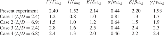
, are measured to be



1. Introduction
A vortex ring is a self-propagating three-dimensional toroidal structure easily observable in nature, ranging from aquatic animal locomotion and jet propulsion (see review by Dabiri (Reference Dabiri2009)) to cardiac flows (Gharib et al. Reference Gharib, Rambod, Kheradvar, Sahn and Dabiri2006). Vortex rings can also be observed in starting jets, pulsed jets and synthetic jets, all of which are used for flow control, unsteady heat and mass transport or thrust generation (see review by Glezer & Amitay (Reference Glezer and Amitay2002)). Understanding the formation of isolated vortex rings, therefore, has significant appeal across a wide range of fields and industrial applications.
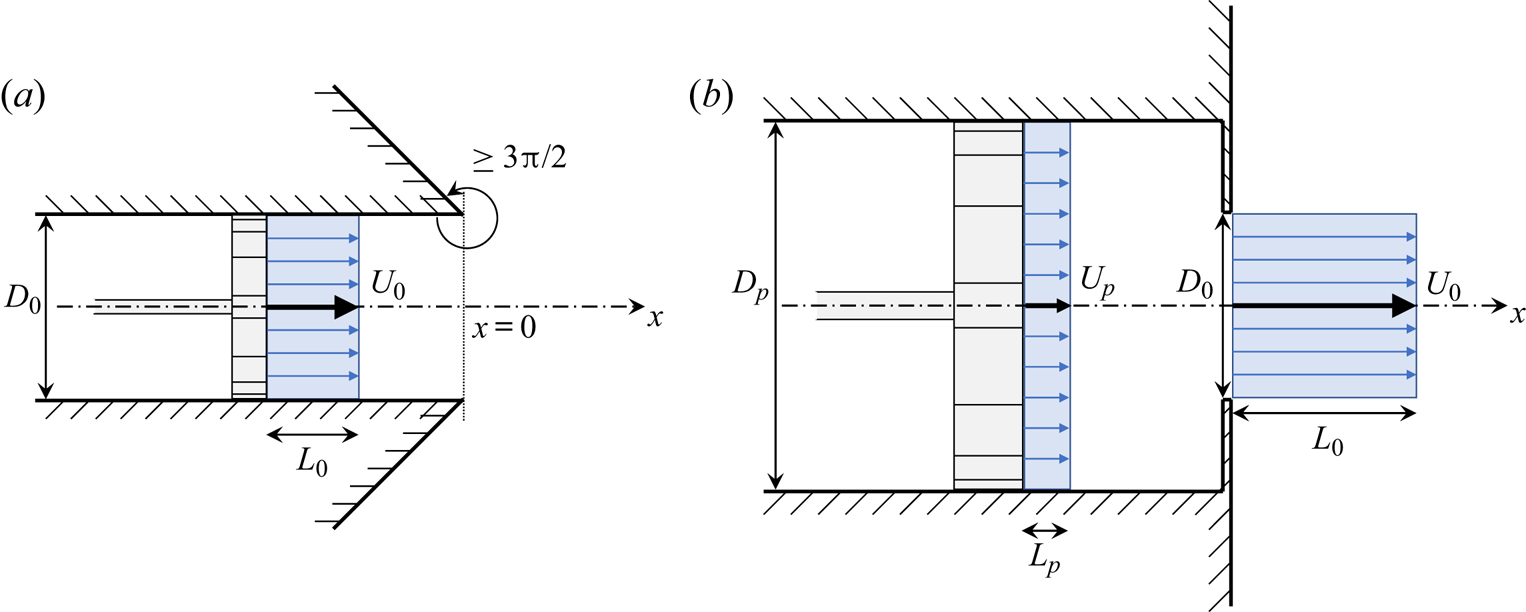
Experimentally, vortex rings are generated by a brief discharge of fluid through a sharp-edged nozzle or orifice, as shown in figure 1. Didden (Reference Didden1979) provided a thorough description of the formation process at the exhaust of a knife-edged nozzle; as the column of fluid is impulsively discharged into the quiescent surroundings, the shear imposed by the turning angle forces the sheet of vorticity to curl and roll up into a vortex ring. Didden (Reference Didden1979) also highlighted secondary effects likely to modify the formation process and the vortex circulation, such as the acceleration of the flow around the edge, the growth of the internal boundary layer or the ingestion of negative vorticity from the outer wall. The simulations of Nitsche & Krasny (Reference Nitsche and Krasny1994) and Heeg & Riley (Reference Heeg and Riley1997) showed overall good agreement with the experiment of Didden (Reference Didden1979), and later direct numerical simulations of viscous laminar vortex rings by James & Madnia (Reference James and Madnia1996) confirmed these findings.
 $(a)$ Nozzle geometry and
 $(b)$ orifice geometry apparatus with simplified slug-flow model at the exhaust. Schematic made to scale for a unit discharge duration.

For short stroke-to-diameter ratios, one isolated vortex ring is generated and all the fluid discharged by the piston/cylinder arrangement is entrained in the rolling motion of the ring. For long stroke ratios, one would observe a leading vortex ring (or puff) followed by a trailing jet. Gharib, Rambod & Shariff (Reference Gharib, Rambod and Shariff1998) were the first to report this limiting process for vortex ring formation with the transition between these two states found to occur at an instantaneous stroke-to-diameter ratio  $L_0(t)/D_0$ of
 $3.6$ to
 $4.5$ for laminar nozzle-generated vortex rings. More precisely, Gharib et al. (Reference Gharib, Rambod and Shariff1998) initially highlighted the critical non-dimensional time during formation to be
 $U_0t/D_0$, where
 $U_0$ is the time-averaged speed at the exhaust, and named it ‘formation time’. This is equivalent to the instantaneous stroke ratio
 $L_0(t)/D_0$. Numerous studies have confirmed this finding for low-speed nozzle-generated vortex rings, suggesting the existence of a universal time scale named ‘formation number’ at which an isolated vortex ring is generated. In particular, Krueger & Gharib (Reference Krueger and Gharib2003) showed that the maximum impulse per unit stroke ratio is obtained at a stroke ratio of
 ${\sim }4$. Following Lawson & Dawson (Reference Lawson and Dawson2013), we prefer the generic term of ‘dimensionless time’ or ‘non-dimensional time’ for the variable
 $t^*=U_0t/D_0$ as it avoids any connotation of universality. Gharib et al. (Reference Gharib, Rambod and Shariff1998) measured the formation number to be the instant at which the maximum circulation of the isolated vortex ring equals the total circulation generated by the apparatus. Invoking the Kelvin–Benjamin variational principle, Gharib et al. (Reference Gharib, Rambod and Shariff1998) proposed an energy-based interpretation for the disconnection of the ring, or ‘pinch-off’. Applied to an incompressible inviscid unbounded axisymmetric flow with zero swirl, the variational method proves that the kinetic energy of a steadily translating vortex ring of fixed hydrodynamic impulse is maximum with respect to any rearrangement of the vorticity distribution preserving the hydrodynamic impulse (Benjamin Reference Benjamin1976). Friedman & Turkington (Reference Friedman and Turkington1981) showed that the condition on the vorticity distribution can be replaced by restrictions on the circulation and the vortex strength. As a consequence, this energy constraint forces the vortex ring to detach from the feeding shear layer once the ring energy has reached its maximum value. As such, the formation number, as defined by Gharib et al. (Reference Gharib, Rambod and Shariff1998), has been interpreted as the instantaneous stroke ratio at which the vortex ring reaches its maximum energy state which coincides with the non-dimensional time at which the maximum ring circulation is attained.
In order to provide a theoretical model for the formation number, the predicted apparent invariants of the motion, namely the kinetic energy  $E$, the hydrodynamic impulse
 $I$ and the circulation
 $\varGamma$, delivered by the nozzle generator and derived from the slug-flow model were equated to their equivalent analytical expression derived for the Fraenkel–Norbury family of isolated vortex rings (Fraenkel Reference Fraenkel1972; Norbury Reference Norbury1973). In order to close the system of equations, one additional assumption is required. Mohseni & Gharib (Reference Mohseni and Gharib1998) estimated the ring speed at the exhaust of the generator by
 $\partial E/\partial I$, derived it from the slug-flow model and matched it to the ring speed. The formation number was then found to be approximately
 $3.0$. Linden & Turner (Reference Linden and Turner2001) argued that the determining constraint is the volume of the ring and found a corresponding formation number of
 $3.5$. Physically, the matching operation defines the formation number to be the instant at which the integrals of the motion delivered by the generator reach those of the isolated vortex ring. An alternative argument can be made using a kinematic interpretation of the pinch-off process. Shusser, Gharib & Mohseni (Reference Shusser, Gharib and Mohseni1999) made use of the thin ring approximation to predict the speed and the diameter of the isolated ring, and estimated the integrals of the motion delivered at the exhaust by the slug-flow model. Hypothesizing that pinch-off occurs when the velocity at the exhaust equates the speed of the isolated thin ring, the formation number was found to be
 $2.96$. Refinement of this method involving the second-order expressions of Fraenkel (Reference Fraenkel1972) for the ring speed and the integrals of the motion was provided, and similar results were found with a predicted formation number of
 $3.08$.
Besides, Mohseni, Ran & Colonius (Reference Mohseni, Ran and Colonius2001) argued that pinch-off results from strong interactions between the vortex ring and the trailing shear layer; as the leading ring grows in size, it pushes the shear layer toward the axis of symmetry and the ring detaches when the local velocity of the shear layer is less than the axial velocity in the ring. Later, Gao & Yu (Reference Gao and Yu2010) described the pinch-off as a relaxation process to an equilibrium state involving two successive phases. First, the ring grows in size at the edge of the nozzle without apparent forward motion and then detaches at the non-dimensional time equal to the formation number. In a second phase, energy is continuously acquired while the ring propagates and the phase terminates with the necking of the trailing jet and the physical disconnection of the leading ring. This follows the comment by Yu, Law & Ai (Reference Yu, Law and Ai2007) that the dynamical approach of Shusser et al. (Reference Shusser, Gharib and Mohseni1999) and the relaxation approach suggested by the Kelvin–Benjamin variational principle do not provide the same result for the occurrence of pinch-off for vortex rings generated by gravity-driven converging nozzles; a vortex ring can still acquire energy, although the ring has attained its maximum circulation, as long as its propagation speed is lower than the exhaust velocity.
Although the formation number appears to be a robust intrinsic state of the flow, with values steadily found around  $4$, it has been shown that initial conditions can drastically affect the value of the formation number. For instance, Rosenfeld, Rambod & Gharib (Reference Rosenfeld, Rambod and Gharib1998) showed that a constant acceleration velocity program yields a formation number of
 $5.22$, whereas a parabolic velocity profile at the exhaust reduces the formation number to
 $0.90$. This value is lower than the
 $1.42$ reported in the simulations of Zhao, Frankel & Mongeau (Reference Zhao, Frankel and Mongeau2000) for a similar initial velocity profile. Moreover, Dabiri & Gharib (Reference Dabiri and Gharib2004) showed that adding a bulk axisymmetric counterflow to the generator delays pinch-off by increasing the amount of circulation the leading ring can ingest, resulting in a larger formation number. In order to model the vortex generation of self-propelled swimmers or vehicles, Krueger, Dabiri & Gharib (Reference Krueger, Dabiri and Gharib2006) showed that the formation number can be reduced to
 $1$ by adding a substantial uniform background coflow. Similarly, Dabiri & Gharib (Reference Dabiri and Gharib2005) studied the dynamics and the formation process of a leading vortex at the edge of a nozzle with temporally varying exit diameter and found that the formation number can be increased to
 $8.0$ by closing the nozzle while ejecting the fluid. Finally, Zhao et al. (Reference Zhao, Frankel and Mongeau2000) showed a strong interaction between the Kelvin–Helmholtz instabilities developing in the trailing jets and the leading vortex ring. They suggested that this interaction can accelerate the pinch-off process and introduces a variation of at least
 $20\,\%$ in the vortex ring circulation and formation number. Gao & Yu (Reference Gao and Yu2012) complemented this study by showing that the development of secondary vortices in a parallel starting jet starts after the formation number is achieved, which is used as an indicator of the final stage of the separation process.
The orifice geometry apparatus (figure 1 $b$) can be used to model complex geometries observed in nature, such as heart valves (Gharib et al. Reference Gharib, Rambod, Kheradvar, Sahn and Dabiri2006) or squids’ funnel (Krueger et al. Reference Krueger, Moslemi, Nichols, Bartol and Stewart2008). Although it is the main apparatus to produce synthetic jets (Glezer & Amitay Reference Glezer and Amitay2002), few studies have used this geometry to generate single vortex rings. It consists of an orifice plate covering the exhaust of a tube or nozzle and may be seen as an infinitely converging nozzle. Unlike nozzle geometries, where the streamlines at the exhaust are parallel with each other, the orifice plate imposes a high turning angle and the radial component of velocity is non-negligible. Rosenfeld, Katija & Dabiri (Reference Rosenfeld, Katija and Dabiri2009) showed numerically the importance of the radial component of velocity in the case of laminar rings generated by conical nozzles of different tube-to-orifice diameter ratios. It was found that the contribution of the radial component of velocity to the circulation reaches
 $44\,\%$ of the total circulation generated. Krieg & Mohseni (Reference Krieg and Mohseni2013a) complemented these findings by measuring the apparent invariants of the flow generated at the exhaust of an orifice. Compared with the equivalent nozzle geometry, it was found that the converging radial velocity leads to an increase of 90–100 % in circulation, 70–75 % in hydrodynamic impulse and 105–135 % in kinetic energy, depending on the stroke ratio. A semiempirical model was provided to account for the radial component of velocity but the formation number was not measured. Furthermore, Yu et al. (Reference Yu, Law and Ai2007) and Gao et al. (Reference Gao, Yu, Ai and Law2008) studied vortex rings emanating from a gradually converging nozzle and found a reduced formation number of
 ${\sim }2$. A model was then provided by Gao & Yu (Reference Gao and Yu2010) which accounts for the presence of a trailing jet and fair agreement with measurements was found.
The objectives of this paper are to investigate the formation process of vortex rings formed with an orifice and determine the critical formation parameters. The details of the experiment and the generation conditions are presented in § 2. Section 3 presents the kinematics of the vortex ring. In § 4, the apparent invariants of the motion generated by the orifice geometry for a set of different stroke-to-diameter ratios and for a fixed Reynolds number are presented. Section 5 focuses on the ring quantities and the non-dimensional numbers used for measuring the formation number. Finally, a comprehensive discussion on the formation process of orifice-generated vortex ring is offered in § 6. The key points raised in the paper are also summarized.
2. Experimental procedure
2.1. Apparatus
Experiments were conducted in a  $2\ \mathrm {m}$ long water tank with a
 $76\ \mathrm {cm}\times 87\ \mathrm {cm}$ cross-sectional area. A
 $127\ \mathrm {mm}$ diameter hole is cut into one end of the tank into which an acrylic tube with a
 $D_p=101.6\ \mathrm {mm}$ inner diameter is mounted. Water is pushed through the tube by an electric actuator (a modified version of ServoCylinder A2, Ultra Motion). The piston has a maximum stroke length of
 $32\ \mathrm {cm}$ and a maximum speed of
 $60\ \mathrm {cm}\ \textrm {s}^{-1}$. The piston head is sealed with rubber O-rings and a silicon-based lubricant is used to reduce friction and eliminate jolts during the initial acceleration. A
 $152.4\ \mathrm {mm}$ diameter flange is attached to the tube and the exhaust is covered with a
 $2.38\ \mathrm {mm}$ thick aluminium sheet into which a
 $D_0=50\ \mathrm {mm}$ orifice is laser cut. The plates were then anodized to prevent spurious reflections of light during particle image velocimetry (PIV) measurements. Because the input to the experiments are the piston speed
 $U_p$, the piston stroke length
 $L_p$ and the orifice diameter
 $D_0$, the speed of the discharged fluid at the exhaust of the orifice
 $U_0$ and the ‘slug length’
 $L_0$ (see figure 1) are computed using the conservation of mass
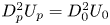 $D^2_pU_p=D^2_0U_0$ or conservation of volume
 $L_pD^2_p=L_0D^2_0$ since density is assumed constant. The temperature of the tank was measured regularly during the measurements and was found to be between
 $20\,^\circ \mathrm {C}$ to
 $23\,^\circ \mathrm {C}$, producing a kinematic viscosity ranging from
 $0.978\ \mathrm {mm}^2\ \textrm {s}^{-1}$ to
 $0.933\ \mathrm {mm}^2\ \textrm {s}^{-1}$. For simplicity, the kinematic viscosity of water is assumed to be
 $1.0\ \mathrm {mm}^2\ \textrm {s}^{-1}$ when computing the Reynolds numbers.
2.2. Velocity program
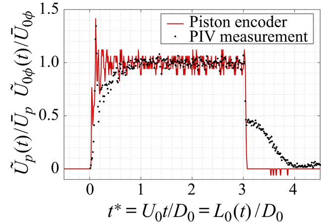
The velocity program of the piston is chosen to be an impulse with maximum acceleration (figure 2). The instantaneous centreline velocity  $\tilde {U}_{0\phi }\equiv \tilde {U}_0(r=0)$ is also shown. The piston velocity program presents a
 $5\,\%$ unsteadiness, defined as the standard deviation about the mean
 $\bar {U}_p=24.2\ \mathrm {mm}\ \textrm {s}^{-1}$, partly due to the limited resolution of the position encoder. The repercussions on the flow speed are minimal as the centreline velocity is measured to have a
 $3\,\%$ unsteadiness about the mean
 $\bar {U}_{0\phi }=103\ \mathrm {mm}\ \textrm {s}^{-1}$. Moreover, although the overshoot in the piston velocity program has a visible impact on the flow field, it is measured to be minimal on the total and ring quantities. The velocity magnitude at the exhaust also exhibits a spike at
 $t^*=0.1$, whose effect is rapidly mitigated with the velocity converging to the prescribed value (figure 2). More precisely, the flow speed gradually increases to reach the target value at a non-dimensional time of approximately
 $t^*=0.8$. This effect can be attributed to internal dynamics, such as recirculating flow upstream of the orifice plate. Finally, when the piston stops, the velocity magnitude drops to a non-zero value, which corresponds to the ambient velocity field generated by the train of vortices downstream. A constant exhaust speed of
 $U_0=100\ \mathrm {mm}\ \textrm {s}^{-1}$ is chosen and the nominal equivalent diameter-based Reynolds number is therefore
 $Re_{D_0}=U_0D_0/\nu =5000$. More precisely, given the kinematic viscosity to be
 $\nu =0.95\pm 0.03\ \mathrm {mm}^2 \ \textrm {s}^{-1}$ and the exhaust speed to be
 $U_0=100\pm 5\ \mathrm {mm}\ \textrm {s}^{-1}$, the diameter-based Reynolds number is closer to
 $Re_{D_0}=5300\pm 400$. Maximum stroke ratios of
 $L_m / D_0 = 0.5$ to
 $5.0$ with a
 $0.5$ increment are investigated and the stroke length Reynolds number
 $Re_{L_m}=U_0L_m/\nu$ varies from
 $2600$ to
 $26\ 000$. The maximum stroke is defined as
 $L_m=\int _{0}^{T_0}\tilde {U}_0(t)\,\mathrm {d}t = L_0(T_0)$, where
 $T_0$ is the duration of the stroke. Note that the stroke length Reynolds number
 $Re_{L_m}=U_0L_m/\nu$ differs from the circulation-based Reynolds number
 $Re_{\varGamma }=U_0L_m/2\nu$ by a factor of
 $1/2$.
Piston velocity program  $U_p$ and centreline velocity at the exhaust
 $U_{0\phi }$. In both cases, the instantaneous velocity
 $\tilde {U}$ is normalized by its corresponding mean value
 $\bar {U}$.

2.3. Velocity profile
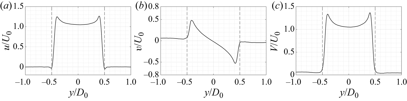
Krieg & Mohseni (Reference Krieg and Mohseni2013a) highlighted the effects of a non-zero radial velocity component on the formation of vortex rings formed by non-parallel starting jets. The available experimental set-up enables measurements at the exhaust  $x=0$ and the velocity profile, as well as the axial and radial components of velocity, are shown in figure 3. The velocity profile is far from uniform and displays high extrema at the edge of the orifice. These velocity profiles are similar to those observed by Didden (Reference Didden1979) who noted a large axial velocity near the edge of a nozzle for small times, causing a large vorticity production and an increase in the overall circulation generated. As time increases, the boundary layer inside a nozzle generator thickens which ultimately gives a parabolic velocity profile. In the case of an orifice, the thickness of the boundary layer is minimal and both radial and axial velocities exhibit extrema at the edge throughout the formation process.
Velocity profile at the exhaust:  $(a)$ axial component;
 $(b)$ radial component; and
 $(c)$ magnitude at a non-dimensional time of
 $t^{*}=2.5$ and for a stroke ratio of
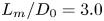 $L_m/D_0=3.0$.

2.4. The PIV set-up
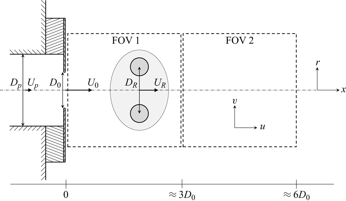
Time-resolved planar PIV is used to study the formation process at the edge of the orifice plate. The position of the high-speed camera (Photron FASTCAM Mini WX50) is adjusted so that it enables the visualization of the roll-up process at the exhaust of the orifice. The field of view (FOV) of size  $16\ \mathrm {cm}\times 16\ \mathrm {cm}=3.2D_0\times 3.2D_0$ extends equally on each side of the axis of symmetry and starts at
 $x=0$ for the first FOV and at approximately
 $3D_0$ for the second FOV (figure 4). The vertical plane containing the axis of symmetry of the ring is illuminated with a high-speed ND:YLF laser (Litron Laser LDY302 PIV series) and the sample rate is adjusted to the piston speed. Both the laser and the camera are triggered by a digital delay generator (Stanford Research System DG645). The PIV processing is performed using DaVis10 software (LaVision GmbH). First, a nonlinear image preprocessing filter consisting in a
 $3\times 3$ pixel sliding-average subtraction is applied to the raw images. Then, a four-pass cross-correlation algorithm is used, ending in a
 $24\times 24\ \mathrm {pixel}$ interrogation window, with
 $50\,\%$ overlap. This results in a
 $170\times 170$ vector field with a spatial resolution of
 ${\rm \Delta} x=1\ \mathrm {mm}=0.02D_0$. No post-processing filtering is applied. Given the vector field, the derivatives of velocity are computed using a finite-difference fourth-order Padé scheme.
Schematic of FOVs considered in the PIV.

In this study, the flow is described by the cylindrical coordinate system  $(x,r,\theta )$ where the
 $x$ axis coincides with the axis of symmetry of the orifice. The velocity vector is denoted
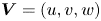 $\boldsymbol {V} = (u,v,w)$,
 $w$ being the out-of-plane velocity assumed to be negligible in the present axisymmetric configuration (figure 4).
A total of seven runs per stroke ratio were taken in the first FOV and four runs per stroke ratio in the second FOV. In the subsequent figures, the confidence interval displayed as error bars are computed using the  $t$ distribution with a
 $97.5\,\%$ confidence.
3. Kinematics of the vortex ring
3.1. Definition of the core centroid
Strictly speaking, the core centroid of a vortex is defined as the point in space where the velocity, in a frame of reference following the vortex, is zero. Experimentally, because the moving vortex ring is visualized in a fixed frame of reference, no point in space has a zero velocity magnitude. For an axisymmetric vortex, Lamb (Reference Lamb1932) defined the centre of vorticity as
 \begin{equation} x_c=\frac{\displaystyle\iint{x r^2\omega\,\mathrm{d}r\,\mathrm{d}\kern0.05em x}}{\displaystyle\iint{r^2 \omega\,\mathrm{d}r\,\mathrm{d}\kern0.05em x}} \quad r_c^2=\frac{\displaystyle\iint{r^2 \omega\,\mathrm{d}r\,\mathrm{d}\kern0.05em x}}{\displaystyle\iint{\omega\,\mathrm{d}r\,\mathrm{d}\kern0.05em x}}, \end{equation}
where the integrals are computed over a surface defining the vortex core. The axial and radial position of the core centroid were estimated using the above (3.1a,b) with a vorticity threshold of  $50\ \mathrm {s}^{-1}$, which corresponds to approximately
 $40\,\%$ of the maximum vorticity value. The diameter of the ring was also determined by measuring the distance between the location of minimum velocity magnitude. This method produced a ring diameter that is
 $5\,\%$ larger, and an axial position that is within
 $1\,\%$, compared with using (3.1a,b). Note that axial position of the centroid is averaged between both the negative and positive vortex cores.
3.2. Position, speed and diameter
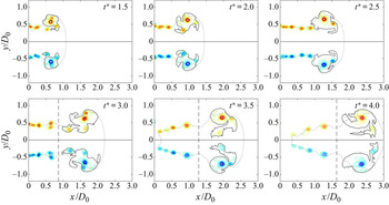
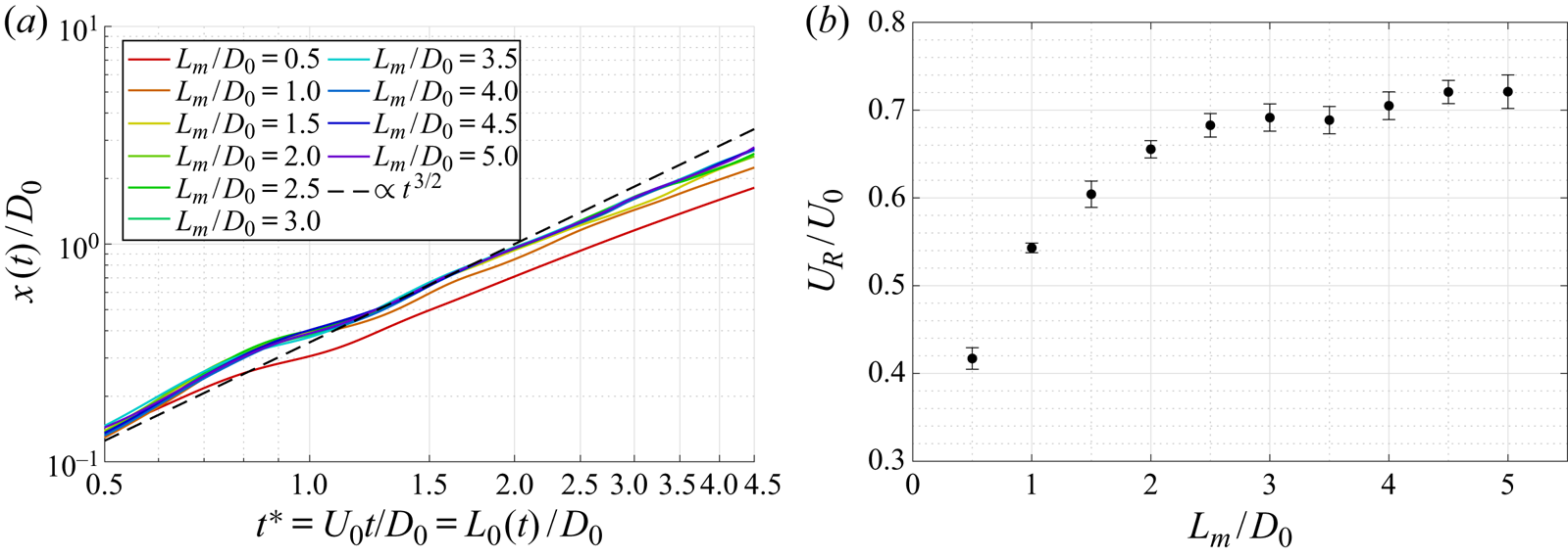
Figure 5 shows the time history vorticity contours of an orifice-generated vortex ring with a stroke ratio of  $3.0$. Shortly after the onset of the piston, a patch of vorticity can be isolated and the vortex centroids can be tracked as the primary ring propagates downstream. One can clearly see that the leading vortex ring does not have a continuous feeding shear layer attached to it, as is observed for nozzle-generated vortex rings. Instead, a trail of separated vortex rings is observed between the orifice and leading vortex. These are likely created due to vortex shedding, as a result of the large turning angle of the orifice plate. Figure 6
 $(a)$ shows the
 $x$ position history of the ring for stroke ratios ranging from
 $0.5$ to
 $5.0$. As the primary ring propagates, it may interact and merge with trailing vortices which translates into wavy
 $x=f(t^{*})$ curves. Nevertheless, by the end of the first FOV, the rings follow a steady path and the slope of the curves corresponds to the normalized axial speed of the ring
 $U_R/U_0$. The position of orifice-generated vortex rings over time follows the same power-law
 $\propto t^{3/2}$ as the laminar nozzle-generated vortex rings studied by Didden (Reference Didden1979), Nitsche & Krasny (Reference Nitsche and Krasny1994), Heeg & Riley (Reference Heeg and Riley1997), James & Madnia (Reference James and Madnia1996) and Mohseni et al. (Reference Mohseni, Ran and Colonius2001). Note that this is in contradiction to the similarity theory of Saffman (Reference Saffman1978) and Pullin (Reference Pullin1978) for starting flow past a sharp edge (nozzle or orifice) which predicts
 $x\propto t^{2/3}$. More precisely, the power law predicts accurately the
 $x$ position of the ring for dimensionless time ranging from
 $1.0$ and
 $2.0$ and breaks down for larger times, which is consistent with the observations of Didden (Reference Didden1979).
Normalized vorticity contours in the first FOV for contour levels of  $\omega D_0/U_0=-50(5)50$, excluding the zero vorticity contour, at non-dimensional times of
 $t^{*}=1.5(0.5)4.0$ and for a stroke ratio of
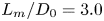 $L_m/D_0=3.0$. The isovorticity contour of
 $\omega =\pm 2\ \mathrm {s}^{-1}$, or equivalently
 $\omega D_0/U_0=\pm 1$, is shown as a solid black line. The isovelocity contour of
 $V/U_0=1$ is shown as a dotted black line. The position of the local minimum of velocity at the centreline is shown as a dashed black line.

 $(a)$ Time history of the axial position of the core centroid and
 $(b)$ axial ring speed
 $U_R/U_0$ as a function of the stroke ratio
 $L_m/D_0$.

As shown in figure 6 $(b)$, the speed of the ring reaches an asymptote of approximately
 $0.7U_0$, consistent with measurements of Krieg & Mohseni (Reference Krieg and Mohseni2013b). This asymptotic value is reached for stroke ratios above
 $2.0$. More precisely, the rings generated at short stroke ratios of
 $L_m/D_0=0.5$,
 $1.0$ and
 $1.5$ clearly deviate at the instant at which the piston stops and ultimately propagates slower (figure 6
 $a$). However, trailing vortices may eventually merge with the primary ring and increase its momentum. For instance, for a stroke ratio of
 $L_m/D_0=1.5$, the ring ends up having a speed of approximately
 $0.7U_0$ in the first FOV but relaxes to a lower speed farther downstream. Figure 6
 $(b)$ suggests a limiting process in the transfer of axial momentum from the generator to the ring; for short-stroke ratios, insufficient momentum is ejected from the generator to form a ring with maximum translational speed.
Given the  $x$ and
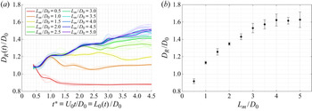
 $r$ positions of the centroids, it is also possible to compute the diameter of the ring by measuring the distance between the two centroids. Figure 7
 $(a)$ shows the time history of the ring diameter. As fluid is pushed through the orifice, the vortex ring grows in diameter and detaches from the exhaust. Similarly to the
 $x$ position history, a point of inflexion is visible at the instant at which the piston stops, e.g. at
 $t^{*}=1.0$ for
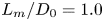 $L_m/D_0=1.0$. For short stroke ratios, the ring detaches and relaxes to a ring smaller than what it was initially. Farther downstream, the ring diameter has reached a steady value and can be plotted as a function of the stroke ratio (figure 7
 $b$). Clearly, the ring diameter increases with the stroke ratio and plateaus to a value of
 $1.6D_0$ at a stroke ratio of
 $L_m/D_0=4.0$.
 $(a)$ Time history of the diameter of the ring and
 $(b)$ ring diameter
 $D_R/D_0$ as a function of the stroke ratio
 $L_m/D_0$.

4. Invariants of the motion: total quantities
The Euler equations of unbounded inviscid incompressible flows have a Hamiltonian structure and possess a total of seven conserved quantities associated with the symmetries of the equations: the hydrodynamic impulse, the angular impulse and the Hamiltonian functional, i.e. the kinetic energy. Additionally, the degeneracy of the Hamiltonian operator leads in three dimensions to the invariance of the helicity, and in two dimensions to the invariance of the area integrals  $\iint f(\omega )\,\mathrm {d}S$, where
 $f$ is any arbitrary function of
 $\omega$. When
 $f$ is the identity function, the area integral reduces to circulation (Olver Reference Olver1982).
4.1. Total circulation
The simplest and most used model to estimate the circulation generated by vortex formation at an exhaust is the slug-flow model, which assumes the discharged fluid to be a uniform slug of fluid with parallel streamlines (Shariff & Leonard Reference Shariff and Leonard1992). Equivalently, one can invoke the thin boundary layer approximation and assume  ${\partial v}/{\partial x} \ll {\partial u}/{\partial r}$. The rate of change of circulation can be related to the flux of vorticity entering the control volume as follows:
 \begin{equation} \frac{\mathrm{d}\varGamma}{\mathrm{d}t} = \frac{\mathrm{d}}{\mathrm{d}t} \iint{\boldsymbol{\omega}\boldsymbol{\cdot}\boldsymbol{\mathrm{d}S}} = \int{ u \left(\frac{\partial v}{\partial x} - \frac{\partial u}{\partial r} \right) \, \mathrm{d}r} = \underbrace{\int{ u \frac{\partial v}{\partial x} \, \mathrm{d}r}}_{(\mathrm{i})} - \underbrace{\int{ u \frac{\partial u}{\partial r}\, \mathrm{d}r}}_{(\mathrm{ii})}, \end{equation}
and the circulation is simply measured as
 \begin{equation} \varGamma = \iint{\boldsymbol{\omega}\boldsymbol{\cdot}\boldsymbol{\mathrm{d}S}} = \iint{\left(\frac{\partial v}{\partial x} - \frac{\partial u}{\partial r} \right) \, \mathrm{d}r\,\mathrm{d}\kern0.05em x} = \underbrace{\iint{\frac{\partial v}{\partial x} \, \mathrm{d}r\,\mathrm{d}\kern0.05em x}}_{(\mathrm{I})} - \underbrace{\iint{\frac{\partial u}{\partial r} \, \mathrm{d}r\,\mathrm{d}\kern0.05em x}}_{(\mathrm{II})}. \end{equation}
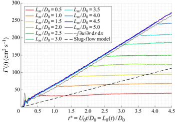
The total circulation is measured as the surface integral of vorticity within the top and bottom half-planes and each contribution is averaged out to give a single value (see (4.2)). As shown in figure 8, the total circulation increases linearly as the fluid is pushed out and remains constant once the piston has stopped. Compared with the equivalent slug-flow model for parallel starting jets, the rate of change of the total circulation generated by an orifice is increased by a factor of  $2.40\pm 0.02$. This value is similar to case 4 of Krieg & Mohseni (Reference Krieg and Mohseni2013a) (table 1). Whereas the slug-flow model was shown to overestimate the total circulation generated by a nozzle (Gharib et al. Reference Gharib, Rambod and Shariff1998), the model drastically underestimates the total circulation generated by non-parallel jets. Krieg & Mohseni (Reference Krieg and Mohseni2013a) and Rosenfeld et al. (Reference Rosenfeld, Katija and Dabiri2009) demonstrated that this increase in circulation is largely due to the non-negligible radial component of velocity in (4.1). Furthermore, as shown in figure 3, the velocity profile exhibits extrema at the edge of the orifice plate throughout the whole formation process owing to both the radial and the axial components, resulting in a larger vorticity production, hence a larger circulation.
Total circulation generated at the exhaust of an orifice of tube-to-orifice diameter ratio  $D_p/D_0=2.0$ for stroke ratios ranging from
 $0.5$ to
 $5.0$.

Comparison of the measured total quantities with the data of Krieg & Mohseni (Reference Krieg and Mohseni2013a). Cases 1 and 2 are nozzle geometries and cases 3 and 4 are orifice geometries. Values were retrieved using the slope of the curves in their figures 16, 17, 18, 19, 21 and 22.

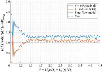
The available set-up enables the measurement of the circulation production at the exhaust, and an estimation of the contribution of each term of (4.1). Figure 9 presents the rate of change of circulation measured at the exhaust normalized by the slug-flow model  $(\mathrm {d}\varGamma /\mathrm {d}t)_{slug}=1/2U_0^2$. The total value of
 $(\mathrm {d}\varGamma /\mathrm {d}t)_{exp.}=2.40\times 1/2U_0^2$ is also shown. First, the second term,
 $(\mathrm {ii})$, of (4.1) follows accurately the slug-flow model which is not surprising since the model is precisely derived from this term. The first term,
 $(\mathrm {i})$, of (4.1), which involves the radial component of velocity, contributes to the remainder of the production of circulation, which is approximately
 $60\,\%$ of the total production. However, when measuring the circulation itself, the contribution of term
 $(\mathrm {I})$ in (4.2) is found to be minimal and the majority of circulation is found in the term with the axial velocity (
 $(\mathrm {II})$ in (4.2)) (figure 8). In short, although the production of circulation is found to be primarily due to the axial gradient of the radial velocity
 $\partial v/\partial x$, the circulation itself is mainly found in the radial gradient of axial velocity
 $\partial u/\partial r$.
Normalized rate of change of circulation for a stroke ratio of  $5.0$.

4.2. Total hydrodynamic impulse
In unbounded flows and in the absence of non-conservative forces, the hydrodynamic impulse remains invariant, which corresponds to the invariance of the Euler equations to spatial displacement (Saffman Reference Saffman1992). The flow being axisymmetric, the vorticity is only in the azimuthal direction and the hydrodynamic impulse reduces to its  $x$ component:
 \begin{equation} I = \rho {\rm \pi}\iint{\omega r^2\,\mathrm{d}r\,\mathrm{d}\kern0.05em x}. \end{equation}
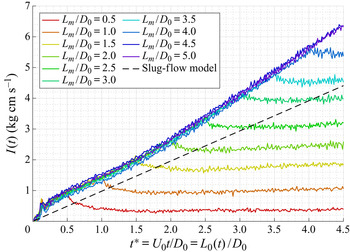
The dimensional total hydrodynamic impulse is plotted as a function of the non-dimensional time for different stroke ratios on figure 10. Similarly to circulation, the measured total hydrodynamic impulse is greater than the predicted slug-flow model, but to a lesser extent. More precisely, the rate of change of impulse is increased by a factor of  $1.52\pm 0.07$ compared with the slug-flow model. This is consistent with the factor
 $1.6$ and
 $1.3$ for cases 3 and 4 of Krieg & Mohseni (Reference Krieg and Mohseni2013a) (table 1).
Total hydrodynamic impulse generated at the exhaust of an orifice of tube-to-orifice diameter ratio  $D_p/D_0=2.0$ for stroke ratios ranging from
 $0.5$ to
 $5.0$.

An inflection point is observed in the total impulse around  $t^*=1.5$ in figure 10, marking the stabilization of the rate of change of impulse. An explanation for the apparent excess of impulse at small dimensionless time is available. As fluid is pushed out at the exhaust, vorticity is generated at the sharp edge of the orifice plate. During the very first instant, the forming ring remains attached to the orifice with the two patches of vorticity being separated by a constant distance of roughly
 $1.1D_0$ for
 $t^*<0.7$, as shown in figure 7
 $(a)$. In other words, the ring does not move but there is production of vorticity. Given that impulse includes the contribution of vorticity weighted by the square of the radial position (see (4.3)), this results in a high hydrodynamic impulse for short dimensionless time. In essence, the ring is artificially larger than it should be for
 $t^*<1.5$, owing to the presence of the orifice plate, which gives rise to a higher than expected impulse.
For short stroke ratios, the forming leading ring is forced to detach from the orifice edge which results in a reduction of size of the ring itself (see figure 7 $a$) and a decrease in hydrodynamic impulse. For long stroke ratios, the primary ring has already detached and propagates downstream. Stopping the piston forces the last trailing ring to detach from the orifice edge, which then moves inwardly due to its own dynamics and the induced velocity of the rings in front of it (see figure 5). As shown in figure 10, this results in a decrease of the overall hydrodynamic impulse shortly after stopping the piston.
The inward dynamics of the leading ring, and subsequent rings, can be linked by the presence of the orifice plate and can be explained by potential flow theory. The wall boundary conditions imposed by the orifice plate can be modelled by fictitious mirror vortices. When the piston stops, no external velocity field is applied and one is left with the dynamics of counter-rotating vortex rings. The mutual interaction of the vortices forces the vortex ring to reduce its diameter and increase its speed. Close to the orifice plate, the hydrodynamic impulse is not conserved as the flow is not unbounded.
4.3. Total kinetic energy
The kinetic energy is another invariant of the flow and corresponds to the invariance of the Euler equations with time (Saffman Reference Saffman1992). In an axisymmetric flow with no swirl, the kinetic energy reduces to
 \begin{equation} E = \rho {\rm \pi}\iint{ (u^2 +v^2) r \,\mathrm{d}r\, \mathrm{d}\kern0.05em x}. \end{equation}
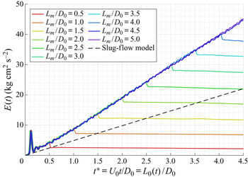
The dimensional total kinetic energy is plotted as a function of the non-dimensional time in figure 11, where energy is seen to increase linearly as the fluid is pushed out from the orifice. Once the piston stops, the kinetic energy remains roughly constant, although it does exhibit a minute decrease over the spatial extent considered here, which is attributed to possible turbulent dissipation. The small dip in the kinetic energy appearing right after  $t^*=L_m/D_0$ is attributed to the sudden stopping of the piston. The rate of change of energy is found to be increased by a factor of
 $2.14\pm 0.04$ compared with the slug-flow model and is comparable with cases 3 and 4 of Krieg & Mohseni (Reference Krieg and Mohseni2013a) which have a factor of
 $2.5$ and
 $2.0$, respectively (table 1).
Total kinetic energy generated at the exhaust of an orifice of tube-to-orifice diameter ratio  $D_p/D_0=2.0$ for stroke ratios ranging from
 $0.5$ to
 $5.0$.

4.4. Total non-dimensional numbers
Given the three integrals of the motion, namely the circulation  $\varGamma$, the hydrodynamic impulse
 $I$ and the kinetic energy
 $E$, along with the characteristic quantities of the system, namely the density of the fluid
 $\rho$, a velocity
 $U$, a diameter
 $D$ and a streamwise length
 $L$, it is possible to define three independent non-dimensional numbers. Taking
 $I$ and
 $\varGamma$ to be the repeated variables, the non-dimensional quantities are the stroke ratio
 $L/D$ and two non-dimensional numbers
 $\alpha$ and
 $\beta$:
 \begin{equation} \alpha = \frac{E}{\rho^{1/2}\varGamma^{3/2}I^{1/2}} \quad \beta = \frac{\varGamma}{\rho^{{-}1/3}I^{1/3}U^{2/3}}. \end{equation}
Employing the classic slug-flow assumption, the total circulation, impulse and energy can be estimated as
 \begin{equation} \varGamma_s(t) = \tfrac{1}{2} U_0 L_0(t), \quad I_s(t) = \tfrac{1}{4} {\rm \pi}\rho D_0^2 L_0(t) U_0, \quad E_s(t) = \tfrac{1}{8}{\rm \pi} \rho D_0^2L_0(t)U_0^2, \end{equation}
and the above non-dimensional quantities become
 \begin{equation} \alpha_s(t) = \sqrt{\frac{\rm \pi}{2}} \left(\frac{L_0(t)}{D_0}\right)^{{-}1}, \quad \beta_s(t) = \frac{1}{(2{\rm \pi})^{1/3}}\left(\frac{L_0(t)}{D_0}\right)^{2/3}. \end{equation}
In addition to these two non-dimensional parameters, and following the argument of Linden & Turner (Reference Linden and Turner2001) on the importance of the volume, another non-dimensional number is defined as

where  is a volume. Making use of the slug-flow model, the volume discharged at the exhaust can be approximated by
 and the non-dimensional number can be written in the slug-flow approximation as
 \begin{equation} \gamma_s =\frac{1}{\sqrt{2{\rm \pi}}}\left(\frac{L_0(t)}{D_0}\right). \end{equation}
The quantities have been derived above for an impulsively started parallel jet. Gharib et al. (Reference Gharib, Rambod and Shariff1998) have shown that drastic changes in the velocity program do not alter the evolution of the non-dimensional number  $\alpha$ in time. However, the influence of the velocity program on the
 $\beta$ quantity was not shown.
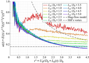
Figure 12 shows the evolution of the non-dimensional number  $\alpha$ for a Reynolds number of
 $Re_{D_0}=5000$ and for different stroke ratios. As predicted by the slug-flow model, the quantity is inversely proportional to
 $L_0(t)/D_0$, but the experimental curve is observed to be shifted downward. Instead of the coefficient
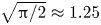 $\sqrt {{\rm \pi} /2}\approx 1.25$ in (4.7a,b), a better fit is obtained with a coefficient of
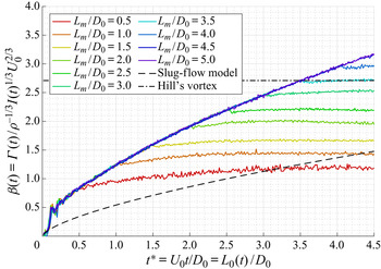
 $0.55\pm 0.02$.Similar comments can be made on the evolution of the total non-dimensional number
 $\beta$ (figure 13). First, because this non-dimensionalization involves the total quantities at the exhaust, the theoretical speed
 $U_0$ is used to define
 $\beta$. Again, the slug-flow model accurately predicts the trend of
 $\beta$ but underestimates its absolute value. Rather than
 $(2{\rm \pi} )^{-1/3}\approx 0.54$ in (4.7a,b), a better fit is obtained with a coefficient of
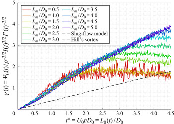
 $1.19\pm 0.02$. Figure 14 shows the evolution of the non-dimensional number
 $\gamma$. After a relaxation period of
 $t^*=2$, the curves follow a linear trend, as predicted by the slug-flow model. A good fit to the curve would be a straight line of slope
 $0.77\pm 0.05$. Interestingly, for short stroke ratios of
 $L_m/D_0=0.5$,
 $1.0$ and
 $1.5$, when the ring clearly does not have a trailing jet, the total
 $\gamma$ quantities are the same with a value of approximately
 $2$.
Total non-dimensional number  $\alpha$ generated at the exhaust of an orifice of tube-to-orifice diameter ratio
 $D_p/D_0=2.0$ for stroke ratios ranging from
 $0.5$ to
 $5.0$.

Total non-dimensional number  $\beta$ generated at the exhaust of an orifice of tube-to-orifice diameter ratio
 $D_p/D_0=2.0$ for stroke ratios ranging from
 $0.5$ to
 $5.0$.

Total non-dimensional number  $\gamma$ generated at the exhaust of an orifice of tube-to-orifice diameter ratio
 $D_p/D_0=2.0$ for stroke ratios ranging from
 $0.5$ to
 $5.0$.

Hill's spherical vortex, which is the limiting member of the Fraenkel–Norbury family of isolated vortex rings, has non-dimensional number values of  $\alpha _H = \sqrt {10{\rm \pi} }/35\approx 0.16$,
 $\beta _H=5/(2{\rm \pi} )^{1/3}\approx 2.71$ and
 $\gamma _H=10/3\sqrt {5/2{\rm \pi} }\approx 2.97$. Given the available set of data, these values are obtained at non-dimensional times of
 $t^*=3.5$,
 $3.5$ and
 $3.3$, respectively (figures 12, 13 and 14).
Finally, the non-dimensional numbers from the study of Krieg & Mohseni (Reference Krieg and Mohseni2013a) can be inferred from their data and compared. The exhaust speeds presented in their table 1 are used to compute  $\beta$ and the volume discharged is estimated by
 ${\rm \pi} /4D_0^2U_0t$ to compute
 $\gamma$. The values are reported in table 1 of this paper. The present measurements corroborate the results of Krieg & Mohseni (Reference Krieg and Mohseni2013a) and highlight the critical differences between straight nozzles and orifice geometries. In all cases, the slug-flow model is found to poorly predict the dimensional and non-dimensional quantities, the difference being less pronounced for the nozzle case.
5. Invariants of the motion: ring quantities
5.1. Methodology
In order to compute the ring quantities, it is necessary to draw a boundary around the ring as it propagates downstream. Strictly speaking, the extent of the vortex core is insufficient since fluid entrained outside the core must be taken into account, as it conveys vorticity and energy. Several approaches to define such a boundary have been proposed. Most studies, including Gharib et al. (Reference Gharib, Rambod and Shariff1998), Gao et al. (Reference Gao, Yu, Ai and Law2008) and Krieg & Mohseni (Reference Krieg and Mohseni2013b), measured the ring quantities within the closed isovorticity contour set at some small vorticity threshold encompassing the primary vortex ring core. In our case, the extent of the leading vortex core is defined as the  $\pm 2\ \mathrm {s}^{-1}$ isovorticity contour containing the peak vorticity, which results in a
 $4\,\%$ difference compared with the
 ${\pm }1\ \mathrm {s}^{-1}$ threshold. A
 $\pm 2\ \mathrm {s}^{-1}$ limit allows us to clearly distinguish the leading ring from the background noise and provides robust post-processing.
A clear separation between the ring and the feeding shear layer is also required to properly define the extent of the vortex ring. For this reason, Gharib et al. (Reference Gharib, Rambod and Shariff1998) measured the ring quantities farther downstream, at a non-dimensional time of  $t^*>7$. In our case, it is possible to isolate the leading vortex ring as early as
 $t^*=2.0$, which corresponds to an approximate distance of
 $1.0$ diameter from the exhaust (figure 5). This allows us to study the early dynamics of the forming ring, especially the merging of secondary rings with the leading ring.
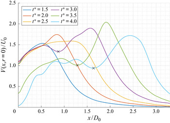
When measuring the kinetic energy of the ring, it is important to take into account not only the rotational velocity inside the vortex ring core but also the irrotational fluid in the entrainment region and the translational speed of the ring. In order to do so, a vertical straight line is drawn between the primary ring and the secondary ring and all the fluid downstream is taken into account when computing the kinetic energy (figure 5). Looking at the velocity magnitude along the centreline on figure 15, the separating line is placed at the position of the trailing local minimum. Lawson & Dawson (Reference Lawson and Dawson2013) showed the role of adverse pressure gradients in the formation process and provided a one-dimensional dynamical model to define the onset of pinch-off. A trailing velocity minimum suggests the presence of a trailing pressure maximum and therefore an adverse pressure gradient. Lawson & Dawson (Reference Lawson and Dawson2013) argued that the appearance of the trailing pressure maximum initiates the disconnection of the ring by terminating the flux of vorticity into the ring.
Evolution of the velocity magnitude at the centreline for a stroke ratio of  $L_m/D_0=3.0$ (case of figure 5). The position of the trailing minimum is shown as a black cross.

5.2. Ring circulation
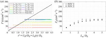
Figure 16 $(a)$ shows the measured circulation of the ring along with the linear fit to the total circulation,
 $\varGamma = 60t^* + 3.8~(\mathrm {cm^2\ s^{-1}})$, obtained using the data from
 $L_m/D_0 = 5.0$ in figure 8. Once the vortex core can be isolated within the
 $\pm 2\ \mathrm {s}^{-1}$ isovorticity limit, and if no trailing rings catch up and merge with the leading ring, the circulation remains constant throughout the first FOV. Increasing the maximum stroke-to-diameter ratio results in a vortex ring with greater circulation until it reaches an asymptotic value of
 $\varGamma _R \approx 120\ \mathrm {cm}^2\ \textrm {s}^{-1}$ for
 $L_m/D_0 \ge 2.5$. Previous studies have measured the formation number as the instant at which the ring circulation intersects the total circulation generated at the exhaust of the apparatus. Using the same definition, the formation number for orifice-generated vortex rings is clearly found to be
 $2.0\pm 0.1$.
Ring circulation for stroke ratios ranging from  $0.5$ to
 $5.0$
 $(a)$ as a function of
 $t^*$,
 $(b)$ as a function of
 $L_m/D_0$.

It is worth noting that for short stroke ratios, i.e.  $L_m/D_0=0.5$,
 $1.0$ and
 $1.5$, the intersection between the ring circulation and the total circulation occurs at a non-dimensional time, or instantaneous stroke ratio, of
 $0.5$,
 $1.0$ and
 $1.5$, respectively, which is consistent with the assumption that all the vorticity generated of the orifice is entrained in the rolling motion of the primary ring. However, for a stroke ratio of
 $2.0$, the intersection between the ring circulation and the total circulation does not give an instantaneous stroke ratio of
 $2.0$, which suggests that the ring has detached from the feeding shear layer before the apparatus has stopped ejecting fluid and some vorticity was left behind. A fortiori, for
 $L_m/D_0 \ge 2.5$, the instantaneous stroke ratio corresponding to the intersection between the ring circulation and the total circulation, which is the definition of the formation number, is less than the actual stroke-to-diameter ratio and it is therefore not surprising to observe a trailing jet in this condition (see figure 5).
When plotting the ring circulation in the first and second FOV as a function of the maximum stroke ratio, shown in figure 16 $(b)$, it is found that the ring circulation reaches the maximum value of
 $120\ \mathrm {cm}^2 \ \textrm {s}^{-1}$ at a stroke ratio of approximately
 $L_m/D_0 \approx 2.5$. Gharib et al. (Reference Gharib, Rambod and Shariff1998) and Zhao et al. (Reference Zhao, Frankel and Mongeau2000) showed a similar plot and found that the maximum ring circulation was obtained for stroke ratios in the range of
 $4.0$ to
 $5.0$. Clearly, the formation of orifice-generated vortex rings differs from nozzle-generated ones, as they pinch-off sooner and reach their circulation asymptotic state for shorter stroke ratio.
5.3. Ring hydrodynamic impulse
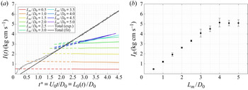
Figure 17 $(a)$ shows the evolution of the hydrodynamic impulse of the ring, calculated within the bounds of the
 $\pm 2\ \mathrm {s}^{-1}$ isovorticity contour, in the first FOV. First, as outlined in § 4.2, the total hydrodynamic impulse does not follow a linear trend for
 $t^*<1.5$ and it is therefore not surprising to note that for short stroke ratios of
 $0.5$ and
 $1.0$, the intersection between the ring hydrodynamic impulse and the measured total quantity does not correspond to the effective quantity of fluid discharged in the tank. However, for a stroke ratio of
 $L_m/D_0=1.5$, the intersection between the ring quantity and the total quantity curves correspond to an instantaneous stroke-to-diameter ratio of
 $L_0(t)/D_0=1.5$ which, as was the case for circulation, shows that all the fluid discharged at the exhaust has been entrained in the primary ring. Figure 17
 $(a)$ also displays the linear fit,
 $I = 1.48t^* -0.327~(\mathrm {kg}\ \mathrm {cm}\ \mathrm {s}^{-1})$ of the total hydrodynamic impulse, calculated using the
 $L_m/D_0=5.0$ data of figure 10. Here, we do see that the ring quantities for
 $L_m/D_0\leq 2.0$ do intersect the fitted line at
 $t^*=L_m/D_0$. For larger stroke ratios, where trailing vortices are clearly present, the ring impulse increases steadily which suggests that the ring has not reached a relaxed state and is still adapting to its own dynamics. In other words, the ring is still gaining impulse but at a smaller rate than it is produced, which is consistent with the findings of Gao & Yu (Reference Gao and Yu2010). However, because the circulation remains constant within the FOV, the increase in impulse is attributed to the radial distribution of vorticity rather than the quantity of vorticity in the core, i.e. circulation (see (4.3)). Also, it can be observed that the growth rate of the ring impulse increases with the stroke ratio for
 $2.5 \leq L_m/D_0 < 4.0$ and seems to remain at a fixed value for
 $L_m/D_0 \geq 4.0$. By extending the increasing ring impulse curves in figure 17
 $(a)$ and alternative measure of the formation number can be obtained.
Ring hydrodynamic impulse for stroke ratios ranging from  $0.5$ to
 $5.0$
 $(a)$ as a function of
 $t^*$,
 $(b)$ as a function of
 $L_m/D_0$.

In the second FOV, the ring has relaxed to its asymptotic state and the ring hydrodynamic impulse remains constant. The values are shown in figure 17 $(b)$ from which we note that the maximum hydrodynamic impulse of
 $I_R \approx 5\ \mathrm {kg}\ \mathrm {cm}\ \mathrm {s}^{-1}$ is obtained for stroke ratios greater than
 $3.5$. By tracing back the instant at which the apparatus has generated this amount of impulse, a non-dimensional time of 3.5–4.0 is found. Therefore, determining the stroke ratio required to generated the maximum impulse can be determined by tracing back the asymptotic value in time to the total curve. However, the results suggest that one would have to wait for at least
 $t^* \approx 6$ to obtain that value.
5.4. Ring kinetic energy
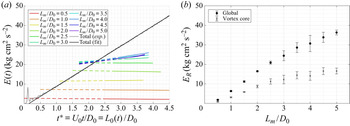
The kinetic energy of the ring as a function of  $t^*$ and
 $L_m/D_0$, is shown in figure 18. The total kinetic energy of the flow is found to follow the linear relationship
 $E=10.3t^*-1.50~(\mathrm {kg}\ \mathrm {cm}^2\ \mathrm {s}^{-2})$. For short stroke ratios
 $L_m/D_0\leq 2.5$, the ring kinetic energy is found to be constant in time, within the FOV, with the asymptotic value increasing linearly with the stroke ratio
 $L_m/D_0$ (figure 18
 $b$). By extrapolating the increasing ring energy curves for
 $L_m/D_0 \geq 2.5$ to the total energy curve, it is possible to retrieve the formation number.
Ring kinetic energy for stroke ratios ranging from  $0.5$ to
 $5.0$
 $(a)$ as a function of
 $t^*$,
 $(b)$ as a function of
 $L_m/D_0$.

Figure 18 $(b)$ highlights the significant difference in the measured energy of the vortex ring when one only considers the core, compared with the method proposed here. Evidently, the fact that the circulation, the hydrodynamic impulse and the kinetic energy of the isolated vortex ring intersect their equivalent total quantities at the same non-dimensional time solidifies our decision to calculate the ring energy in the manner described above. However, one does observe that there is no clear plateau in the ring energy as the stroke ratio increases, although one could argue that the data does plateau, within the error bars, for
 $L_m/D_0 \ge 4$ (figure 18
 $b$). Note that this is consistent with the value obtained for the impulse (figure 17
 $b$). Additional data would need to be collected at larger
 $L_m/D_0$ to discern if there is a plateau for the ring energy for large stroke ratio. Nevertheless, the data does suggest that an isolated vortex ring would not reach its maximum energy state unless a stroke ratio of
 $L_m/D_0 \geq 4$ is used. This has significant implications on the definition and process of vortex ring formation, which shall be addressed further in § 6. The asymptotic energy of the isolated vortex ring is found to be
 $E_R\approx 35~(\mathrm {kg}\ \mathrm {cm}^2\ \mathrm {s}^{-2})$, and the non-dimensional time at which the apparatus generates this amount of energy, found as the intercept with the total energy curve, is approximately
 $t^* = 3.5$. Finally, the available growth rate of the ring energy suggests that the asymptotic value of the ring energy would be met at a non-dimensional time later than
 $t^* = 7$.
5.5. Non-dimensional quantities
The non-dimensional quantities  $\alpha$ and
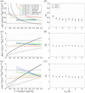
 $\beta$ have been shown to be suitable quantities to characterize the behaviour of isolated vortex rings (Gharib et al. Reference Gharib, Rambod and Shariff1998; Mohseni & Gharib Reference Mohseni and Gharib1998). The variation of this parameter for an isolated vortex ring for different stroke ratios in the second FOV is shown in figure 19
 $(b)$, where the
 $\alpha$ quantity is found to be approximately
 $\alpha _R=0.33\pm 0.03$ for stroke ratios greater than
 $1.5$. The asymptotic value of
 $\alpha _R \approx 0.33$ is consistent with the previous experimental results of Gharib et al. (Reference Gharib, Rambod and Shariff1998), Gao et al. (Reference Gao, Yu, Ai and Law2008) and Krieg & Mohseni (Reference Krieg and Mohseni2013b), simulations of Zhao et al. (Reference Zhao, Frankel and Mongeau2000), Mohseni et al. (Reference Mohseni, Ran and Colonius2001) and Danaila & Hélie (Reference Danaila and Hélie2008) and analytical predictions of Mohseni & Gharib (Reference Mohseni and Gharib1998), Linden & Turner (Reference Linden and Turner2001) and Kaplanski & Rudi (Reference Kaplanski and Rudi2005). The consistency among these studies suggests that the
 $\alpha$ quantity is a robust measure of isolated vortex rings and might be a fixed value for all vortex rings. The intersection between the
 $\alpha$ quantity of the isolated vortex ring
 $\alpha _R\approx 0.33$ and the total measured quantity gives a non-dimensional time of
 $t^{*}=1.7\pm 0.2$ (figure 19
 $a$). This intersection can again be interpreted as the instantaneous stroke ratio required to generate an isolated vortex ring.
Ring non-dimensional numbers for stroke ratios ranging from  $0.5$ to
 $5.0$
 $(a,c,e)$ as a function of
 $t^*$,
 $(b,d,f)$ as a function of
 $L_m/D_0$.

Similar comments can be made with the non-dimensional quantity  $\beta$ which, unlike the
 $\alpha$ quantity, involves the kinematics of the ring via its speed. In the second FOV, the ring
 $\beta$ quantity is found to be
 $\beta _R=1.8\pm 0.1$ (figure 19
 $d$), consistent with the measurements of Gharib et al. (Reference Gharib, Rambod and Shariff1998) (information provided by Mohseni & Gharib (Reference Mohseni and Gharib1998)), the simulations of Mohseni et al. (Reference Mohseni, Ran and Colonius2001) and Danaila & Hélie (Reference Danaila and Hélie2008) and the analytical predictions of Mohseni & Gharib (Reference Mohseni and Gharib1998), Linden & Turner (Reference Linden and Turner2001) and Kaplanski & Rudi (Reference Kaplanski and Rudi2005). Interestingly, while a predicted value of
 $\alpha _R\approx 0.33$ provides an accurate estimation of the formation number for nozzle-geometries by means of the slug-flow model, an inconsistency is found concerning the
 $\beta$ quantity. The estimated
 $\beta$ quantity of the isolated vortex ring of
 $1.77$ (Mohseni & Gharib Reference Mohseni and Gharib1998) would not intersect the slug-flow model curve before
 $t^*=5.8$. Given the available set of measurements of orifice-generated vortex rings, the intersection of the ring
 $\beta$ quantity of
 $\beta _R\approx 1.8$ with the measured total quantity curve occurs at
 $t^{*}=1.8\pm 0.1$ (figure 19
 $c$).
Similarly to  $\beta$, the quantity
 $\gamma$ incorporates the ring circulation, the hydrodynamic impulse and the kinematics of the ring, this time via its volume. In order to compute the volume of the ring atmosphere (or ‘bubble’), the separating streamline is necessary. The volume of the ring in its asymptotic state is estimated another way. First of all, recalling figure 14 of § 5.5, it is possible to see that for short stroke ratios, the
 $\gamma$ quantity remains close to a value of
 $2$. However, for these short stroke ratios of
 $L_m/D_0=0.5$,
 $1.0$ and
 $1.5$, no trailing jet is observed and all the fluid discharged is entrained in the rolling motion of the leading ring. As a consequence, the definition of the ring volume in the second FOV must match the total volume discharged and give a value close to
 $2$ for short stroke ratios, and provided that the portion of ambient fluid entrained remains minor. When estimating the ring volume by its diameter cubed, the ring
 $\gamma$ quantity is found to be constant to a value of approximately
 $\gamma _R\approx 1.9$ for all stroke ratios (see figure 19
 $f$). This is close to the value measured in the first FOV and this can be taken as an initial estimation of the ring
 $\gamma$ quantity in the second FOV. Finally, by finding the intersection of the ring
 $\gamma$ quantity
 $\gamma _R\approx 1.9$ with the total
 $\gamma$ quantity, a non-dimensional time of
 $1.9\pm 0.1$ is found (figure 19
 $e$).
6. The formation process
The results indicate that the formation process of orifice-generated vortex rings differs from nozzle-generated vortex rings primarily due to the high turning angle imposed by the orifice plate which disturbs the flow and influences the early dynamics of the leading ring. It is worth recalling that the tube-to-orifice diameter ratio in this study is 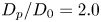 $D_p/D_0=2.0$. As the ratio tends to one, the influence of the radial component of velocity on the production of the invariants of the motion is expected to reduce, hence meeting the assumptions of the slug-flow model. The temporal evolution of an orifice starting jet at a Reynolds number of
 $Re_{D_0}=5000$ and a stroke ratio of
 $L_m/D_0 = 3.0$ is presented in figure 5. Snapshots at four instants
 $t^*=1.0$,
 $2.0$,
 $3.0$ and
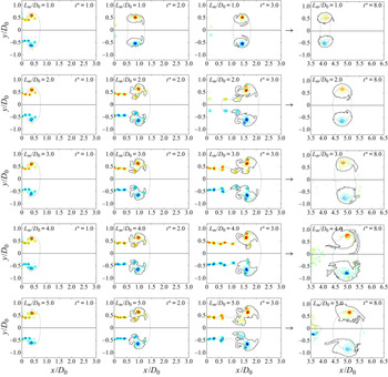
 $8.0$ are presented for the same Reynolds number and for five different stroke ratios in figure 20.
Normalized vorticity contour in the first FOV for contour levels of  $\omega D_0/U_0=-50(5)50$, excluding the zero vorticity contour, at non-dimensional times of
 $t^{*}=1.0$,
 $2.0$,
 $3.0$ and
 $8.0$, for stroke ratios of
 $L_m/D_0=1.0(1.0)5.0$. The isovorticity contour of
 $\pm 2\ \mathrm {s}^{-1}$, or equivalently
 $\omega D_0/U_0=\pm 1$, is shown as a solid black line. The isovelocity contour of
 $V/U_0=1$ is shown as a dotted black line.

When the flow is impulsively started and fluid is pushed out of the orifice into the quiescent surrounding fluid, and in order to satisfy the Kutta condition at the edge, the vortex sheet separates and rolls up in the form of a vortex ring. The orifice geometry differs from nozzle geometries and (gradually) converging nozzles because the boundary layer only develops on the thickness of the orifice plate and is therefore insignificant. The boundary layer inside the tube, however, is expected to grow and separate at the corner of the orifice plate, hence forming a recirculation region upstream of the orifice. As shown in § 2.3, this results in the exhaust velocity profile exhibiting extrema at the edge of the orifice throughout the whole formation process, even for long stroke ratios. Additionally, there is a non-negligible radial velocity component (see figure 3 $b$) which, according to (4.1), increases the production of circulation compared with parallel starting jets (see figure 9). As a consequence, unlike low-speed nozzle geometries which produce a continuous shear layer, the orifice generates a discrete train of vortices which interact with each other and eventually merge with the leading vortex ring long after it has detached from the orifice edge. The secondary vortices are due to vortex shedding, as opposed to Kelvin–Helmholtz instabilities for nozzles (Zhao et al. Reference Zhao, Frankel and Mongeau2000), and appear very early on in the formation process.
As highlighted by Gharib et al. (Reference Gharib, Rambod and Shariff1998), and expanded upon by Gao & Yu (Reference Gao and Yu2010), the formation of vortex rings is not an instantaneous event and it is therefore necessary to precisely define the different stages during formation, as well as the time scales and quantities at stake. By taking the intercept of the asymptotic ring quantities with the total quantities, not only different limiting non-dimensional times compared with nozzle-generated vortex rings were observed, but also differences in the stroke ratio generating the vortex ring with maximum circulation, impulse or energy. The following section aims at defining the critical time scales and quantities of orifice-generated vortex rings.
6.1. Formation number, optimal formation time and optimal stroke ratio
6.1.1. Non-dimensional time or ‘formation time’
The non-dimensional time  $t^*$ is typically defined as
 $U_0t/D_0$, where
 $U_0$ is the exhaust speed and
 $D_0$ the orifice or nozzle diameter, and it is synonymous with the instantaneous stroke ratio
 $L_0(t)/D_0$, where
 $L_0(t)$ is the length of the column (or slug) of fluid discharged through the exhaust at time
 $t$. For temporally varying velocity profiles, for instance when a non-impulsive velocity program is used, or temporally varying diameter, an integral definition can be used instead:
 \begin{equation} t^* = \int_{0}^{t}\frac{U_0(\tau)}{D_0(\tau)}\,\mathrm{d}\tau. \end{equation}
Dabiri (Reference Dabiri2009), followed by Gao, Guo & Yu (Reference Gao, Guo and Yu2020), proposed a general definition for the non-dimensional time as
 \begin{equation} t^* = \int_{0}^{t}\frac{C(\tau)}{U_0(\tau)D_0(\tau)} \frac{\mathrm{d}\varGamma}{\mathrm{d}\tau}\,\mathrm{d}\tau \end{equation}
where  $C = U_0^2(\mathrm {d}\varGamma /\mathrm {d}t)^{-1}$ is a generator-specific coefficient. Given the rate of production of circulation of
 $(\mathrm {d}\varGamma /\mathrm {d}t)_{exp.}=2.40\times 1/2U_0^2$, the present orifice geometry gives
 $C\approx 0.83$ compared with nozzles which have
 $C\approx 2$, according to the slug-flow model. This apparatus-driven parameter provides a measure of how fast the apparatus is able to generate circulation; hence the orifice apparatus generates circulation at a faster rate than the nozzle geometry. In the present case of an impulsively started piston with a constant diameter, and using a semiempirical version of the slug-flow model as shown in § 4.1, i.e.
 $\mathrm {d}\varGamma =2.40\times 1/2U_0^2\mathrm {d}t$, the above definition of the non-dimensional time reduces to
 $t^*=U_0t/D_0$. It is therefore reasonable to assume that
 $C$ is a function of the tube-to-orifice diameter ratio
 $D_p/D_0$. However, the relationship is left for future study.
6.1.2. Detachment time  $t_d^*$

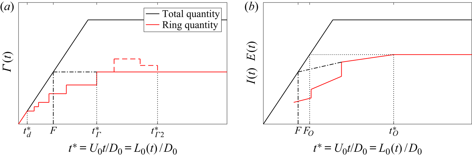
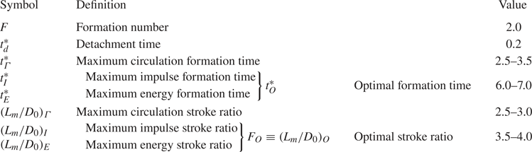
As early as  $t^*=0.2$, it is possible to isolate a pair of vorticity patches, indicating that the vortex ring has ‘detached’ from its feeding shear layer; this time is labelled
 $t^*_d$ in figure 21 and table 2. Although the primary ring remains in the vicinity of the orifice edge and has no apparent forward motion, the ring gains its circulation in a stepwise manner. In previous literature, pinch-off is defined as the instant at which the leading ring ceases to entrain mass or vorticity from the starting jet (Gharib et al. Reference Gharib, Rambod and Shariff1998; Dabiri Reference Dabiri2009). This definition is misleading in the case of orifice-generated vortex rings as circulation is accumulated in a discrete fashion by secondary vortex rings. Therefore, the authors prefers the term ‘detachment time’ for the instant at which the leading ring disconnects from the starting jet in the vorticity sense.
Simplified evolution of  $(a)$ the circulation and
 $(b)$ the hydrodynamic impulse and kinetic energy.

Definitions of critical formation parameters observed during the formation process of an orifice-generated vortex ring.

6.1.3. Maximum circulation formation time $t_\varGamma ^*$

For short stroke ratios, i.e. 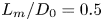 $L_m/D_0=0.5$,
 $1.0$ and
 $1.5$, the leading ring detaches from the orifice edge, relaxes to a smaller ring and propagates due to its own dynamics. This can be qualified as an isolated vortex ring and no trailing jet is observed (see figure 20). The speed of the ring and the ring quantities remain constant in time (see figures 16
 $a$, 17
 $a$ and 18
 $a$). For long stroke ratios, the flow exhibits a train of vortices, from which the leading ring can be identified. Although the primary ring has started propagating downstream, it continues to acquire circulation from secondary vortices. At some later time, the last trailing ring merges with the primary ring and the circulation of the leading vortex ring is fixed; this corresponds to
 $t^*_\varGamma$ in figure 21 and we refer to this as the maximum circulation formation time. It corresponds to the time one has to wait in order for the vortex ring to reach its asymptotic circulation, after which it will not take on any additional circulation. This value is naturally larger than the formation number, ranging from
 $t^*_\varGamma =2.5$ to
 $3.5$ in our experiments. Because of the specific initial conditions of the orifice geometry, the ring begins propagating soon after the onset of the piston, and the ring circulation remains below the optimal circulation state. In the event of excess circulation being ingested (as reported by Gharib et al. (Reference Gharib, Rambod and Shariff1998) or Yu et al. (Reference Yu, Law and Ai2007)), the leading ring would release vorticity in the wake to reach the optimal circulation state (
 $t^*_{\varGamma 2}$). This state was not observed in our measurements.
6.1.4. Maximum circulation stroke ratio $(L_m/D_0)_\varGamma$

The formation number  $F$ is defined as the non-dimensional time at which a vortex ring starts exhibiting a trailing jet. Gharib et al. (Reference Gharib, Rambod and Shariff1998) showed that for a nozzle-generated vortex, the formation number coincides with the instant at which the ring circulation attains its maximum value. For an orifice geometry, the formation number, as the instant at which the ring circulation intersects the total circulation curve, is found to be
 $F=2.0\pm 0.2$ (figure 16
 $a$). Comparing with the set of snapshots of figure 20, this corresponds to the limiting stroke ratio at which a trailing jet starts to appear. When looking at the evolution of the ring circulation as a function of the stroke ratio in figure 16
 $(b)$, the maximum circulation is obtained for a stroke ratio of approximately
 $(L_m/D_0)_\varGamma =2.5\text {--}3.0$. However, the temporal evolution of the vortex shown in figure 5, clearly indicates that a trailing jet is obtained for a maximum stroke ratio of
 $L_m/D_0 = 3.0$ (also visible in measurements with
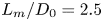 $L_m/D_0=2.5$, not shown here). As such, the value of the formation number does not coincide precisely with the stroke ratio producing the ring with maximum circulation, implying that there are some losses in the system. Similar observations were made for a nozzle geometry by Gharib et al. (Reference Gharib, Rambod and Shariff1998) who found that the instant at which the maximum ring circulation is reached, i.e. the formation number of
 $t^*=3.6\text {--}4.5$, is slightly less than the maximum stroke ratio required to produce these rings, which was found to be 4–5.
6.1.5. Maximum impulse formation time $t_I^*$

Similarly, in the early stages of formation, the hydrodynamic impulse contained in the leading ring increases in a stepwise manner. Given that the hydrodynamic impulse is related to the radial distribution of vorticity (see (4.3)), the relaxation dynamics of the leading ring via the ring diameter is also visible. For large stroke ratios, the impulse increases steadily after ingesting the last secondary ring, with the ring adapting its diameter rather than its speed, as shown in figures 6 and 7. After a certain amount of time, the ring hydrodynamic impulse plateaus and reaches its asymptotic state; this time is referred as ‘maximum impulse formation time’  $t^*_I$. Using the results from figure 17, we find that
 $t^*_I \approx 6$. Note, that this is not equivalent to requiring a stroke ratio of
 $L_m/D_0 \approx 6.0$ for the ring to obtain its maximum impulse, which we see from figure 17
 $(b)$ to occur for
 $( L_m/D_0 )_I \approx 3.5\text {--}4.0$. This limiting stroke ratio
 $(L_m/D_0 )_I$ can also be determined by extrapolating the asymptotic value of the ring to the total curve.
6.1.6. Maximum energy formation time $t_E^*$

Since the kinetic energy of the ring can also be related to the radial distribution of vorticity, similar conclusions to that of hydrodynamic impulse can be made here. Although the ring has physically detached from the trailing train of vortices, in the vorticity sense, the ring has not pinched-off in the velocity sense. This is shown in the velocity magnitude at the centreline of figure 15 and in the contour plots of figures 5 and 20 where the contour level for  $V = U_0$ is not closed around the leading vortex ring before
 $t^* \approx 3.5$. This corroborates the findings of Yu et al. (Reference Yu, Law and Ai2007) and Gao & Yu (Reference Gao and Yu2010). As a consequence, the leading ring can still acquire energy, although the ring has detached from the trailing train of vortices. As was the case for the hydrodynamic impulse, the non-dimensional time at which the isolated vortex ring reaches its maximum energy state is estimated to be approximately
 $t^*_E\approx 7$ and is referred as maximum energy formation time. The stroke ratio required to obtain this maximum state for the isolated vortex ring is
 $(L_m/D_0 )_E \approx 3.5\text {--}4.0$ and can be retrieved from the total energy curve.
6.1.7. Optimal formation time $t_O^*$ and Optimal stroke ratio $F_O\equiv (L_m/D_0)_O$


It is reasonable to assume that the maximum impulse formation time  $t^*_I$ and the ‘maximum energy formation time’
 $t^*_E$ are identical with a value around
 $t^*\approx 6\text {--}7$; this time corresponds to the instant at which the ring reaches its optimal state. It is named as the ‘optimal formation time’ and is labelled
 $t^*_O$ in figure 21. Moreover, the stroke ratios
 $( L_m/D_0 )_I$ and
 $( L_m/D_0 )_E$ required to produce a ring with optimal ring impulse and energy are the same and referred as ‘optimal stroke ratio’. It was found to be
 $F_O\equiv ( L_m/D_0 )_O\approx 3.5\text {--}4.0$. In both cases (impulse and energy), and as shown in figure 21, the formation number
 $F$ can be found by extrapolating the increasing ring quantity curves to the total curve, and a value of
 ${\sim }2$ is found.
As shown in figure 21, the formation number  $F$ of orifice-generated vortex rings falls between the initial detachment time
 $t^*_d$ and the non-dimensional times
 $t^*_\varGamma$ and
 $t^*_O$. Looking at the contour plots at a non-dimensional time equal to the formation number of
 $2.0$, it is clear that the formation number does not correspond to a critical time of the physics of the flow. However, the formation number accurately predicts the instantaneous stroke ratio at which the starting jet starts exhibiting a trailing jet.
6.2. Kelvin–Benjamin variational principle and the formation process
Critical to understanding the use of the Kelvin–Benjamin variational principle, in the context of the asymptotic matching proposed by Gharib et al. (Reference Gharib, Rambod and Shariff1998) to determine the formation number, is that it does not consider the dynamics of the vortex ring, only the final state of the ring. More precisely, using the formulation of Friedman & Turkington (Reference Friedman and Turkington1981), the variational principle shows that for an axisymmetric flow with prescribed impulse, bounded circulation and vortex strength, there exists a maximum energy state. Given that the theory entails the three invariants of motion, the non-dimensional variable  $\alpha$ has been used to predict the asymptotic ring state. The common interpretation is that a single steady vortex ring will be created as long as the
 $\alpha$ quantity remains above the limiting value of steady vortex rings, i.e. the formation process is then considered incomplete.
As can be seen from figure 19 $(b)$, the ring
 $\alpha$ quantity plateaus to a value of
 $\alpha _R=0.33\pm 0.03$ for
 $L_m/D_0 \ge 2.5$ for our configuration. This value is consistent with those found in the literature, adding to the notion of universality for the ring
 $\alpha$ quantity. The time at which the ring
 $\alpha$ quantity intercepts the total quantity curve is
 $t^*\approx 2$, and coincides with the formation number
 $F$. One obtains the same result using the two other non-dimensional ring parameters
 $\beta _R\approx 1.8$ and
 $\gamma _R\approx 1.9$. Upon closer examination of the ring
 $\alpha$ quantity, it is found that it reaches this state as soon as
 $t^*=2.5$ (figure 19
 $a$). Note that Gao & Yu (Reference Gao and Yu2010) define the time at which the ring
 $\alpha$ equals the asymptotic value of
 $0.33$ as the ‘separation time’, which they argued is when the vortex ring has separated from the bulk flow in a velocity sense, marking the end of the pinch-off process. This is clearly not the case here, since the vortex separates, in a velocity sense, at
 $t^*_O \approx 6\text {--}7$. Hence the definition used by Gao & Yu (Reference Gao and Yu2010) is inconsistent with our observations. Although the ring has reached its asymptotic value of
 $\alpha _R\approx 0.33$, the energy and impulse of the ring are still increasing (see figures 17
 $a$ and 18
 $a$ ).
In order to explain this observation, we consider the dynamics of the vortex ring as a Hamiltonian system. We focus our discussion solely on the dynamics of vortex rings generated for stroke ratios  $L_m/D_0 > 3$ from
 $t^*_\varGamma$ to
 $t^*_O$, that is to say the case when the circulation of the vortex ring is constant, with both energy and impulse increasing, and
 $\alpha$ constant to
 $\alpha _R\approx 0.33$. Beyond
 $t^*_O$, for all cases, the kinetic energy of the ring is maximum and both it and the hydrodynamic impulse remain constant, which is in-line with the Kelvin–Benjamin variational principle. Roberts (Reference Roberts1972), using the Hamiltonian formalism, demonstrated that the translational speed of isolated vortex rings with an arbitrary axisymmetric vorticity distribution, can be estimated by the relation
 $\delta E=U\delta I$, or in the limit
 $U=\partial E/\partial I$. Moreover, the Hamiltonian representation is known to be equally valid for interacting vortex rings and leapfrogging rings, provided that the rings remain coaxial and axisymmetric (Saffman Reference Saffman1992). The latter two cases are comparable to the early vortex formation stage considered here, whereas the former is appropriate for later stages of the ring. In the range
 $t^*_\varGamma < t^* < t^*_O$, the last trailing ring has merged with the leading ring and the trailing train of vortices is weakly influencing the dynamics of the primary ring. The Hamiltonian of the system can thus be approximated by the kinetic energy of the primary ring alone. Also, it can be verified that the vorticity distribution remains axisymmetric, although the rings are in the process of coalescing. Following the framework of Roberts (Reference Roberts1972), the ring speed can therefore be estimated by
 $U\approx \partial E/\partial I$, which is found to be approximately
 $\partial E/\partial I=0.5U_0$, compared with
 $0.7U_0$ measured experimentally.
Therefore, in the range  $t^*_\varGamma <t^*<t^*_O$ where both the ring hydrodynamic impulse and kinetic energy are increasing, the vortex ring is in the process of reaching its Kelvin–Benjamin energy maximum while maintaining the ring
 $\alpha$ quantity constant to
 $0.33$, and this in a Hamiltonian framework of constant translational speed. In other words, during this time, the vortex ring is adapting its diameter (see figure 7) in order to accumulate the excess energy produced by the generator and keep
 $\alpha$ constant to
 $\alpha _R\approx 0.33$. The omnipresence of
 $\alpha _R\approx 0.33$ in the literature suggests that it is a stable, self-preserving state of the vortex. Eventually the vortex ring reaches a maximum energy state, at
 $t^* = t^*_O$, after which it translates with constant circulation, impulse and energy.
In closing, it is important to reiterate some of the subtleties in what each of the results are showing and how one might conduct a future experiment in order to determine all the parameters. As highlighted by Gharib et al. (Reference Gharib, Rambod and Shariff1998), Gao & Yu (Reference Gao and Yu2010) and Gao et al. (Reference Gao, Guo and Yu2020), the intercept of the ring  $\alpha$ quantity with the total
 $\alpha$ curve indicates only the stroke ratio required for an isolated vortex ring to form, i.e. the formation number
 $F$. A vortex ring having a
 $\alpha _R = 0.33$, however robust and universal, does not imply that the vortex has reached its maximum energy state for a particular system. To find the maximum energy state, one would have to look at the variation of the ring kinetic energy independently. Given the robustness of the limiting value
 $\alpha _R = 0.33$, the lower formation number observed in the present investigation can be explained by the fact that the apparatus generates the invariants of motion at a much faster rate than those observed in nozzle apparatus. Our findings suggest that in order to determine both the optimal formation time
 $t^*_O$ and optimal stroke ratio
 $F_O=(L_m/D_0)_O$ in the case of orifice geometries, without the need to investigate a series of
 $L_m/D_0$ values, it would be prudent to use as large a
 $L_m/D_0$ value as possible and ensure that measurements are taken for
 $t^* = 2 L_m/D_0$ to ensure that the full formation process is observed.
As mentioned earlier, it is reasonable to assume that  $C$ in (6.2) is a function of
 $D_p/D_0$. Although this scaling will affect
 $t^*$ quantitatively, indeed possibly returning a universal formation number of 4, the various formation times scales associated with the discrete vortex formation processes observed here would still hold true and merely scale with
 $t^*$. For instance, given the tube-to-orifice ratio of
 $D_p/D_0=2.0$, one could argue that the non-dimensional time should be multiplied by two which would give the classic value of 4 for the formation number. However, the optimal formation time
 $t_O^*$ would become 13. Regardless of the scaling, it is clear that the formation process of orifice-generated vortex rings differs from nozzle-generated ones.
7. Concluding remarks
The formation process of orifice-generated vortex rings was thoroughly investigated using time-resolved PIV for stroke ratios  $L_m/D_0$ ranging from
 $0.5$ to
 $5.0$, where
 $L_m$ is the maximum stroke length and
 $D_0$ is the orifice diameter, at a fixed Reynolds number of
 $Re_{D_0} = U_0 D_0 / \nu = 5000$, where
 $U_0$ is the constant exhaust speed at orifice. Consistent with previous measurements by Krieg & Mohseni (Reference Krieg and Mohseni2013a), the three invariants of the motions: the circulation
 $\varGamma$; the hydrodynamic impulse
 $I$; and the kinetic energy
 $E$, were found to increase by
 $140\,\%$,
 $50\,\%$ and
 $110\,\%$, respectively, compared with the equivalent slug-flow model for parallel starting jets.
By varying the maximum stroke ratio  $L_m/D_0$, it was possible to determine the asymptotic values for the ring speed, diameter, circulation, hydrodynamic impulse and kinetic energy. The ring speed and circulation reached their asymptotic values at a maximum stroke ratio of approximately
 $L_m/D_0 \approx 2.5\text {--}3.0$, whereas the energy, impulse and diameter reached their asymptotic values at
 $L_m/D_0 \approx 4.0$. The non-dimensional ring parameters had asymptotic values of
 $\alpha _R = 0.33$,
 $\beta _R = 1.8$ and
 $\gamma _R = 1.9$, the latter shown here for the first time. All three were found to be constant for
 $L_m/D_0 \ge 2.5$. The intercept of these ring quantities with their equivalent total curves, generated by the apparatus, allowed us to define two critical formation parameters. The formation number, defined as the non-dimensional time, or instantaneous stroke ratio, at which the vortex ring starts exhibiting a trailing jet, was found to be
 $F \approx 2$. This value was found using the maximum ring circulation
 $\varGamma _R$ and the asymptotic value
 $\alpha _R = 0.33$, consistent with the definitions used in the literature. Finally, the instant at which the ring impulse and energy deviated from the total quantity curve is also a good indication of the formation number. Given the apparent universality of
 $\alpha _R = 0.33$, the lower formation number for orifice-generated vortex rings can be explained by the increased rate at which the invariants of the motion are produced by the apparatus.
Although using a short stroke ratio would produce a single vortex ring, that vortex ring would not have its maximum allowable energy and circulation. The maximum stroke ratio required to obtain this condition, which we term the optimal stroke ratio  $F_O$, is found using the ring hydrodynamic impulse and kinetic energy, and is found to be
 $F_O \approx 4$. In other words, if one required a single vortex ring with no trailing wake, the maximum stroke ratio they should use is
 $L_m/D_0 = 2 \equiv F$, whereas if one requires a single vortex ring with maximum energy then the minimum stroke ratio required is
 $L_m/D_0 = 4 \equiv F_O$, however, there would be a trailing jet.
A detailed analysis of the formation process itself was conducted, by examining the time-varying behaviour of these quantities, which allowed us to define several critical non-dimensional times during the formation process. First, the vortex ring was seen to detach very early on in the formation process, at a non-dimensional time of  $t^* = 0.2 \equiv t^*_d$. The time at which the isolated leading vortex obtained its maximum circulation, termed the ‘maximum circulation formation time’ was found to be
 $t^*_\varGamma = 2.5$, whilst time at which the vortex would obtain its maximum energy and impulse, termed the optimal formation time, was found to be
 $t^*_O \approx 6-7$. This also coincided with the time at which the vortex ring had separated from the trailing jet in a velocity sense. Critically, we showed that all three time scales are greater than the formation number.
The robustness of  $\alpha _R = 0.33$, observed for both orifice and nozzle-generated vortex rings, suggests some form of universality in the formation process and the asymptotic state of experimentally generated vortex rings. Evidently, one would expect the formation parameters found here to tend towards those of a nozzle-generated vortex ring as the ratio between the orifice diameter to the piston diameter tended towards one, which is left for a future investigation.
Funding
Financial support from the Natural Sciences and Engineering Research Council of Canada (NSERC) is gratefully acknowledged.
Declaration of interest
The authors report no conflict of interest.