INTRODUCTION
The world population is increasing by 200 000 per day (Anon. 2011c ). Alexandratos & Bruinsma (Reference Alexandratos and Bruinsma2012) predict a 60% increase in demand for agricultural production by 2050 and demand for cereals is projected to increase to 3 billion tonnes – an increase of 43% from today's 2·1 billion tonnes (Anon. 2009). In terms of the world's most important crops by production quantity, barley (Hordeum vulgare) is ranked fourth amongst the cereals after maize, rice and wheat (Newton et al. Reference Newton, Flavell, George, Leat, Mullholland, Ramsay, Revoredo-Giha, Russell, Steffenson, Swanston, Thomas, Waugh, White and Bingham2011), and represents 0·6 of the land area devoted to cereal production in Ireland (Anon. 2011b ). Optimizing the performance of crops in areas of high yield potential is one possible approach to help meet the future increases in demand whilst minimizing global land use change.
Cereal production in Ireland is predominantly located in, but not restricted to, the south and east of the country where there are higher temperatures and solar radiation hours and less precipitation than in the west and northwest. Based on data from the period 2000 to 2009, Ireland achieves the second highest yields of barley in the world at 6·6 t/ha (Anon. 2011a ). This is despite the fact that over 0.85 of the Irish barley crop is spring-sown barley (Anon. 2011b ), which over the period 1985–2013 had a yield 0·82 that of winter-sown barley in Ireland (Anon. 2014). Spring-sown barley varieties in Ireland are generally two-row type barleys. Total barley yield increases in Ireland of 0·20 and 0·28 on the previous decade were achieved in the 1970s and 1980s, respectively (Anon. 2011a ). Yield increases of 12 and 7% on the previous decade were achieved in the 1990s and 2000s, respectively (Anon. 2011a ), indicating that the rate of yield increase is slowing.
Yield of small grain crops is the product of two components – grain number and grain weight. Grain number in barley is highly correlated with yield across a range of environments (Gallagher et al. Reference Gallagher, Biscoe and Scott1975; Baethgen et al. Reference Baethgen, Christianson and Lamothe1995; Abeledo et al. Reference Abeledo, Calderini and Slafer2003; del Moral et al. Reference del Moral, del Moral, Molina-Cano and Slafer2003; Blake et al. Reference Blake, Bingham, Foulkes and Spink2006; Bingham et al. Reference Bingham, Blake, Foulkes and Spink2007a ; Peltonen-Sainio et al. Reference Peltonen-Sainio, Kangas, Salo and Jauhiainen2007; Serrago et al. Reference Serrago, Alzueta, Savin and Slafer2013). Barley has the capability to produce a surplus of assimilate for grain filling from post-anthesis photosynthesis and pre-anthesis storage reserves (Gallagher et al. Reference Gallagher, Biscoe and Scott1975; Habgood & Uddin Reference Habgood and Uddin1983; Wade & Froment Reference Wade and Froment2003; Bingham et al. Reference Bingham, Blake, Foulkes and Spink2007a ). This has led to the conclusion that grain number largely determines, and as such limits, yield in barley and that further yield increases may be achieved through an increase in grain number. The study environments that have established this strong relationship between grain number and yield in barley include Argentina, Spain, Finland and the UK where average yields for the period 2000–2009 ranged from 2·8 to 5·8 t/ha (Anon. 2011a ). It is unclear whether grain number is also a yield-limiting factor in high-yield potential climates such as Ireland. Relatively cool moist but bright conditions prior to flowering may result in a large number of grains set and it is unclear whether crops in such environments can produce enough assimilate to support the filling of large numbers of grain.
If grain number is a yield-limiting factor in high-yielding environments, it has not been established what physiological or morphological traits must be targeted by agronomists and/or breeders in order to increase grain number. Grain number per unit area of barley is influenced not only by ear number per unit area (Gallagher et al. Reference Gallagher, Biscoe and Scott1975; Grausgruber et al. Reference Grausgruber, Bointner, Tumpold and Ruckenbauer2002; Abeledo et al. Reference Abeledo, Calderini and Slafer2003), but also grain number/ear (Gallagher et al. Reference Gallagher, Biscoe and Scott1975; Arisnabarreta & Miralles Reference Arisnabarreta and Miralles2008b ).
The rapid ear growth period during stem extension is crucial for grain number determination in wheat through its influence on grain number/ear (Fischer Reference Fischer1985; Abbate et al. Reference Abbate, Andrade, Culot and Bindraban1997; Reynolds et al. Reference Reynolds, van Ginkel and Ribaut2000; Miralles & Slafer Reference Miralles and Slafer2007). In barley, grain number/ear is similarly influenced by growth during the stem extension period (Willey & Holliday Reference Willey and Holliday1971; Habgood & Uddin Reference Habgood and Uddin1983; Grashoff & dAntuono Reference Grashoff and dAntuono1997), where some of the spikelets or florets initiated pre-stem extension will die at a young age (Kirby Reference Kirby1973, Reference Kirby1977; Gallagher et al. Reference Gallagher, Biscoe and Scott1975; Waddington & Cartwright Reference Waddington and Cartwright1983; Kirby & Appleyard Reference Kirby and Appleyard1984). Stem extension is a phase where there is a large increase in total crop growth rate (Kirby Reference Kirby1977) and significant spikelet mortality can occur due to a shortage of photosynthate (Richards Reference Richards2000; Arisnabarreta & Miralles Reference Arisnabarreta and Miralles2008a ) and nitrogen (N) (Baethgen et al. Reference Baethgen, Christianson and Lamothe1995) or in response to changes in environmental conditions, namely interception of photosynthetically active radiation (PAR) (Fischer Reference Fischer1985; Reynolds et al. Reference Reynolds, Foulkes, Slafer, Berry, Parry, Snape and Angus2009) and photoperiod (Gambín & Borrás Reference Gambín and Borrás2010). However, grain number/ear is relatively less variable in barley than in wheat. Wheat can compensate for low tiller numbers by increasing grain number/ear due to the high number of potentially fertile florets produced per spikelet, whereas in barley each spikelet contains only one floret (Wade & Froment Reference Wade and Froment2003). Therefore, the influence of grain number/ear on overall grain number per unit area may be less in barley than in wheat, and the influence of ear number per unit area may have a stronger bearing on overall grain number (Arisnabarreta & Miralles Reference Arisnabarreta and Miralles2008a ).
The final number of fertile ears is usually determined slightly before anthesis (Gallagher et al. Reference Gallagher, Biscoe and Scott1975; Slafer et al. Reference Slafer, Kantolic, Appendino, Miralles, Savin, Sadras and Calderini2009). The pattern of tillering generally reported in the literature involves a rapid increase following the emergence of the third leaf on the main stem, reaching a maximum around the beginning of stem extension as the crop moves into the floral initiation stage of development (del Moral et al. Reference del Moral, Ramos and Recalde1984). This is followed by a period of tiller death, which largely occurs during the period from the start of stem extension until anthesis (del Moral et al. Reference del Moral, Ramos and Recalde1984; Gallagher et al. Reference Gallagher, Biscoe and Scott1975) and beyond which shoot number remains stable until harvest (del Moral et al. Reference del Moral, Ramos and Recalde1984; Gallagher et al. Reference Gallagher, Biscoe and Scott1975; Slafer et al. Reference Slafer, Kantolic, Appendino, Miralles, Savin, Sadras and Calderini2009). A flush of late tillering is possible, for example in response to a rainfall event following a period of drought (Jamieson et al. Reference Jamieson, Martin, Francis and Wilson1995), but the contribution of these late tillers to yield is usually thought to be negligible (Kirby Reference Kirby1967; Thorne & Wood Reference Thorne and Wood1988). Similar to spikelet mortality, competition for limited resources during stem extension can result in tiller mortality leading to reductions in the number of potential ears per unit area (Gallagher et al. Reference Gallagher, Biscoe and Scott1975, Reference Gallagher, Biscoe and Scott1976; Kirby Reference Kirby1977). Around the beginning of stem extension, main shoot photoassimilate translocation shifts away from the tillers and towards the main stem itself (Lauer & Simmons Reference Lauer and Simmons1985) and unless tillers have reached a size sufficient to independently produce the photoassimilates they require, they may die (Kirby Reference Kirby1977). Aside from the obvious influence of the quantity of light on the amount of assimilate available per shoot, light quality may also influence shoot death. Reflection of far-red light from neighbouring plants has been shown to both reduce tiller production (Skinner & Simmons Reference Skinner and Simmons1993; Davis & Simmons Reference Davis and Simmons1994) and promote tiller mortality (Sparkes et al. Reference Sparkes, Holme and Gaju2006). Also, N availability during stem extension has been related to shoot mortality in barley (Wamser & Mundstock Reference Wamser and Mundstock2007) and wheat (Sylvester-Bradley et al. Reference Sylvester-Bradley, Stokes and Scott2001).
There is a degree of overlap between the periods of determination of ear number and grain number/ear. If these two sub-components are competing for the same limited supply of resources there may be some trade-off between them, whereby the growth of one is maintained at the expense of the other. The relative importance of each sub-component for determination of overall grain number per unit area is unclear. Understanding the mechanistic relationship that exists between the individual sub-components of grain number and whether this is driven by resource availability will be important for tailoring agronomic practices and breeding strategies aimed at increasing grain number.
The high yields of spring barley in Ireland are achieved against a backdrop of high seasonal yield variability, which during the first decade of the current century ranged from 6·6 to 8·6 t/ha (Anon. 2012). It is clear that environment × genotype interactions are important in any physiological crop study (Gallagher et al. Reference Gallagher, Biscoe, Dennis-Jones, Wright and Wynn-Williams1983). The balance between source (the amount of carbon assimilate available for grain filling) and sink capacity (storage capacity of the grain) during grain filling will vary depending upon environmental conditions and season (Grashoff & dAntuono Reference Grashoff and dAntuono1997; Serrago et al. Reference Serrago, Alzueta, Savin and Slafer2013). Quantifying crop growth and development in commercial cereal crops of barley across several sites and seasons using the same cultivar provides a dataset where the relative contributions of source or sink limitation to grain yield can be studied (Spink et al. Reference Spink, Foulkes, Gay, Bryson, Berry, Sylvester-Bradley, Semere, Clare, Scott, Kettlewell and Russell2000; Blake et al. Reference Blake, Bingham, Foulkes and Spink2006; Bingham et al. Reference Bingham, Blake, Foulkes and Spink2007a , Reference Bingham, Blake, Foulkes and Spink b ). A detailed programme of assessments like this was carried out on a two-row spring barley variety across several sites and seasons in Ireland to aid the identification of factors that determine yield in a high-yielding environment. The following hypotheses were tested:
-
1. Grain number of spring sown-barley determines yield in a temperate maritime climate with high yield potential.
-
2. Grain number of a two-row spring barley variety is most readily influenced by ear number.
MATERIALS AND METHODS
The materials and methods described below are based on those of similar work carried out in the UK on winter barley (Blake et al. Reference Blake, Bingham, Foulkes and Spink2006; Bingham et al. Reference Bingham, Blake, Foulkes and Spink2007a ).
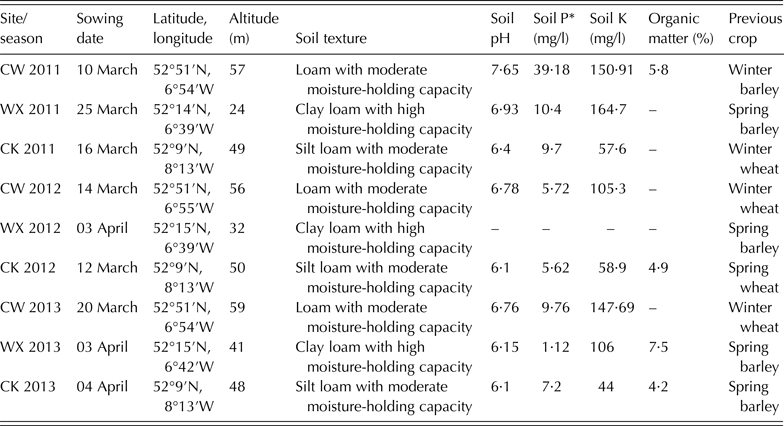
Experimental design and site characterization
Six plots were marked out from commercially grown crops of spring barley at three sites in Ireland (Oak Park, Co. Carlow (CW), Duncormick, Co. Wexford (WX) and Fermoy, Co. Cork (CK), Table 1) across three growing seasons (2011–13). The sites were sheltered, relatively flat and in continuous arable rotations. Meteorological data, including daily rainfall; daily maximum, minimum and mean air temperature; total incident solar radiation; soil temperatures and humidity were obtained from national meteorological stations close to the three sites (maximum distance of 10 km). A high-yield potential two-row malting spring barley variety (H. vulgare cv. Quench) was used due to its strong overall performance in the Department of Agriculture, Food and the Marine (DAFM) Recommended Variety List (Anon. 2011d ).
Sowing date, latitude/longitude, altitude and soil properties for the three experimental sites: Oakpark, Co. Carlow (CW), Duncormick, Co. Wexford (WX) and Fermoy, Co. Cork (CK)

– Missing data.
* Soil P determined by Morgans method.
At each site, three plots for destructive sampling were alternated with three plots for in-field assessments within one bank of six plots. Plots were 4 m wide and ranged in length from 21 to 24 m depending on the distance between the grower's tramlines. The experiments were in a standard barley rotation and were managed for high yield potential using preventative measures to keep the crop free of pests and disease. All soil sampling and nutrient applications were as per best practice outlined by Alexander et al. (Reference Alexander, Black, Boland, Burke, Carton, Coulter, Culleton, Dillon, Hackett, Humphreys, Keady, Lalor, McHoul, Merfield, Murphy, O'Kiely, O'Riordan, Orlovious, Plunkett, Schulte and Tunney2008). Where possible, topsoil samples (0–15 cm) were taken prior to sowing in each season for nutrient status analyses including phosphorous (P), potassium (K), pH, organic matter and micronutrients. Any deficiencies were addressed with compound applications pre-sowing and/or throughout the season. Nitrogen applications of 135–150 kg/ha were the maximum permitted in Nitrates Directive SI 610, 2010, which accounted for the N index of the soil and previous farm yields. Applications were split between early post-emergence when tramlines became visible and during tillering. Fungicides were applied shortly before stem extension and at ear emergence. Applications of aphicide and herbicide were as required. Crops were sown at a rate of approximately 350 seeds/m2 from early March to early April according to local conditions with the aim of achieving a plant stand of 250–300 plants/m2. Further site details are given in Table 1.
In-field assessments
The date of plant emergence was recorded as the first date on which the drilled rows could be clearly seen. Plant population counts were carried out at full crop emergence. The crop was visited regularly thereafter (approximately weekly) and stages of plant development or crop growth stage (GS) were recorded as per the Zadoks decimal scale outlined in Tottman (Reference Tottman1987). The rapid progression through the GSs, typical of spring barley varieties, led to the extrusion of anthers (GS61) coinciding with a developmental stage when half of the ear had emerged on half of all shoots (GS55). This GS is referred to as GS55/61.
To determine the phyllochron, the main stems of 30 plants were tagged and the number of new fully emerged leaves (ligule visible) was recorded at each site visit. The total number of potentially fertile shoots per plant was also recorded on the same 30 plants until harvest. A shoot was counted when its prophyl (protective sheath) or first leaf had emerged by 1 cm from its subtending leaf sheath. These assessments were carried out at each site visit until physiological maturity and again at harvest. Radiation interception by the crop was determined at each site visit by simultaneously measuring radiation above and below the canopy using a Sunscan Canopy Analysis System (Delta-T Devices, Cambridge, UK) as described by Bingham et al. (Reference Bingham, Blake, Foulkes and Spink2007a ).
Destructive sampling
The plots for destructive sampling and subsequent growth analysis were sampled approximately weekly from emergence to physiological maturity. A quadrat sample size of 6 × 1 m2 adjacent row lengths of crop was removed from the field, which equated to 0·72 m2. Samples were stored in sealed plastic bags in order to prevent drying out. If the subsequent growth analysis in the laboratory was delayed, samples were stored in a cold room at 4–6 °C. Sub-samples for dry matter determination were dried at 70 °C to a constant mass and analysed for total N with a Leco FP 328 autoanalyser (LECO Corporation, St. Joseph, MI, USA). Projected green area was determined using a WD3 – WinDIAS Leaf Image Analysis System (Delta-T Devices, Cambridge, UK).
A further quadrat sample was removed just prior to harvest (note: there was no pre-harvest growth analysis sample taken in CK in 2011). A sub-sample (0·2 of the total, by shoot number) was separated into ears and straw for the calculation of yield components. Ears were then hand-threshed between two pieces of foam board and sieved over a mechanically operated 1 mm slotted sieve (Glasbläserei, Institute for Fermentation and Biotechnology, Berlin, Germany) to separate into chaff and grain portions. Material was re-dried before the dry weight of each portion was recorded. Mean grain weight (MGW) was also calculated for each plot using an automated grain counter (Pfeuffer GmbH, Kitzingen, Germany) by counting the number of grains in an approximate 25 g grain sample. After counting, grain weight was determined to the nearest 0·1 mg. Hand threshed grain yield (t/ha) was then expressed at 85% dry matter, grain number/m2 calculated using MGW and plot yield data, and grain number per ear calculated using grain number data and ear number data.
Assessment of lodging and ear blight
Lodging was assessed just prior to harvest or after a lodging event by estimating the proportion of the plot in each of the five categories: upright; leaning (0°–5°); lodged (5°–45°); lodged and flat (45°–90°); brackled (if the stem breaks >0·25 up its length from the base). The visible presence of ear blight (associated with various Fusarium spp. (Osborne & Stein Reference Osborne and Stein2007)) in 2012 across the three sites prompted an in-field assessment of its severity during grain filling when the proportion of the area affected on 25 ears per plot was assessed.
Further analysis of data
Phyllochron was calculated by plotting the number of emerged leaves on the main stem against thermal time from the first assessment. Thermal time was calculated (for this and other assessments) with a base temperature of 0 °C and as per method one of McMaster & Wilhelm (Reference McMaster and Wilhelm1997), below which it is assumed no development occurred (Frank & Bauer Reference Frank and Bauer1995; Kirby Reference Kirby1995; Miralles et al. Reference Miralles, Ferro and Slafer2001; McMaster et al. Reference McMaster, Wilhelm, Palic, Porter and Jamieson2003; Paynter et al. Reference Paynter, Juskiw and Helm2004). A simple linear regression was carried out on the data from each site using GenStat, 14th Edition (VSN International Ltd. Hemel Hempsted, UK) and the phyllochron was then estimated as the reciprocal of the gradient of the fitted line as per Blake et al. (Reference Blake, Bingham, Foulkes and Spink2006).
Total above-ground crop and ear dry biomass were plotted against thermal time from sowing at each site/season. Ear biomass was used as a proxy for grain weight because, after anthesis, the increase in ear biomass is almost entirely accounted for by filling of the grains (Gallagher et al. Reference Gallagher, Biscoe and Scott1975). The start and end of the periods of rapid linear growth were estimated from logistic regressions fitted to these plots using GenStat. These time points were determined according to Bingham et al. (Reference Bingham, Blake, Foulkes and Spink2007b ), where the equation of the curve was differentiated with respect to time to give the instantaneous rate of biomass or ear growth. The start and end points of the rapid linear growth period were then identified as the points at which the percentage change in rate in the accelerating and decelerating phases (either side of the linear phase) were minimized. The dates and developmental stages at which these points occurred were calculated.
Polynomial regressions (second order) were fitted to plots of Green Area Index (GAI) against thermal time from sowing for each site/season using Microsoft Excel (2010) to determine maximum GAI values and estimate green area thermal time duration (GATTD) post-anthesis. Early season data points (pre-GS 31) and late season data points (<0·5 GAI) were omitted from the plots in order to remove ‘tails’ and enable a better fit for the polynomial curve at the maximum. Post-anthesis GATTD was estimated as the area under the graph from GS 55/61 to senescence and expressed as GAI °C days.
To estimate pre-anthesis PAR interception (PARint) the transmitted (below canopy) and incident (above canopy) radiation values were used to calculate the fraction of radiation intercepted by the canopy and interpolated for the days in between each sample date. The daily total incident radiation value from the nearby meteorological station was then multiplied by the fractional interception to calculate daily absolute PARint. Photosynthetically active radiation was estimated as 0·5 × solar radiation (McCree Reference McCree, Lange, Nobel, Osmond and Ziegler1981).
An extinction coefficient (k) for canopy PAR transmission was calculated from values of fractional PARint and GAI measured at anthesis (Bingham et al. Reference Bingham, Blake, Foulkes and Spink2007a ). The value of k varied with each site/season. Post-anthesis fractional PARint by healthy green tissue was then estimated using GAI data from destructive samples during grain filling and canopy senescence and the site/season specific extinction co-efficient (k) determined at anthesis (Bingham et al. Reference Bingham, Blake, Foulkes and Spink2007a ). This approach overcomes difficulties in measuring PAR interception by green tissue during canopy senescence directly, but assumes that canopy architecture and the extinction coefficient do not change after anthesis. This is considered to be a reasonable simplifying assumption until late in the grain filling period (Bingham et al. Reference Bingham, Blake, Foulkes and Spink2007a ). Daily PARint was then calculated as described for pre-anthesis time points.
Radiation use efficiency (RUE; g/MJ) was estimated from linear regressions of accumulated intercepted photosynthetically active radiation (PARint) v. accumulated dry matter plotted for each site/season from GS31 onwards where biomass began to accumulate at a rapid rate. Both split-line and single line regressions were carried out on these data using GenStat to investigate best fit and whether RUE declined or levelled off post-anthesis. Where significant non-linearity of these plots occurred post-anthesis, maximum potential post-anthesis RUE was estimated from the initial linear portion of the regression (Bingham et al. Reference Bingham, Blake, Foulkes and Spink2007a ). Where an average value of post-anthesis RUE was required to investigate the source of dry matter for grain filling in crops of large grain number/m2, linear regressions were fitted to all data points from GS55/61 onwards and RUE was calculated as above.
Yield, yield component and maximum leaf number per main stem were analysed for site, season and site × season effects using a general ANOVA treatment structure with GenStat. The model was as follows: season + site + season × site + site/block. Block was nested in site to account for the fact that blocks at one site were distinct from blocks at another site. Ear blight data for the sites in 2012 were also assessed for site effects in this way.
A similar model was used to test whether differences between mid-season minimum shoot numbers and harvest ear numbers across sites and seasons were significant. An additional timing factor with two levels was added (minimum or harvest). The model was as follows: season + site + timing + season × site × timing + site/block.
To test the hypothesis that the chances of a shoot surviving to form an ear is related to its size and potential to capture resources at the start of stem extension, linear regression analysis was carried out on shoot survival from the early-season maximum shoot number to the identified mid-season minimum shoot number using various measures of shoot weight, size and N content at GS 31, along with other measures of growth before and during stem extension as the explanatory variable. Data for CW 2013 were excluded from these analyses for reasons discussed later.
To investigate the mechanisms by which crops of higher grain number/m2 are able to meet the grain demand for dry matter, linear regression analysis was carried out on several post-anthesis growth variables for all nine site/seasons of data v. grain number/m2. The utilization of stored water soluble carbohydrate was estimated from the decline in stem biomass from anthesis to physiological maturity (GS 55/61–GS 87).
RESULTS
Climatic conditions
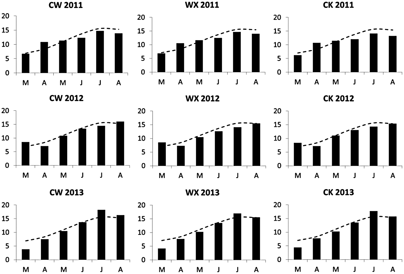
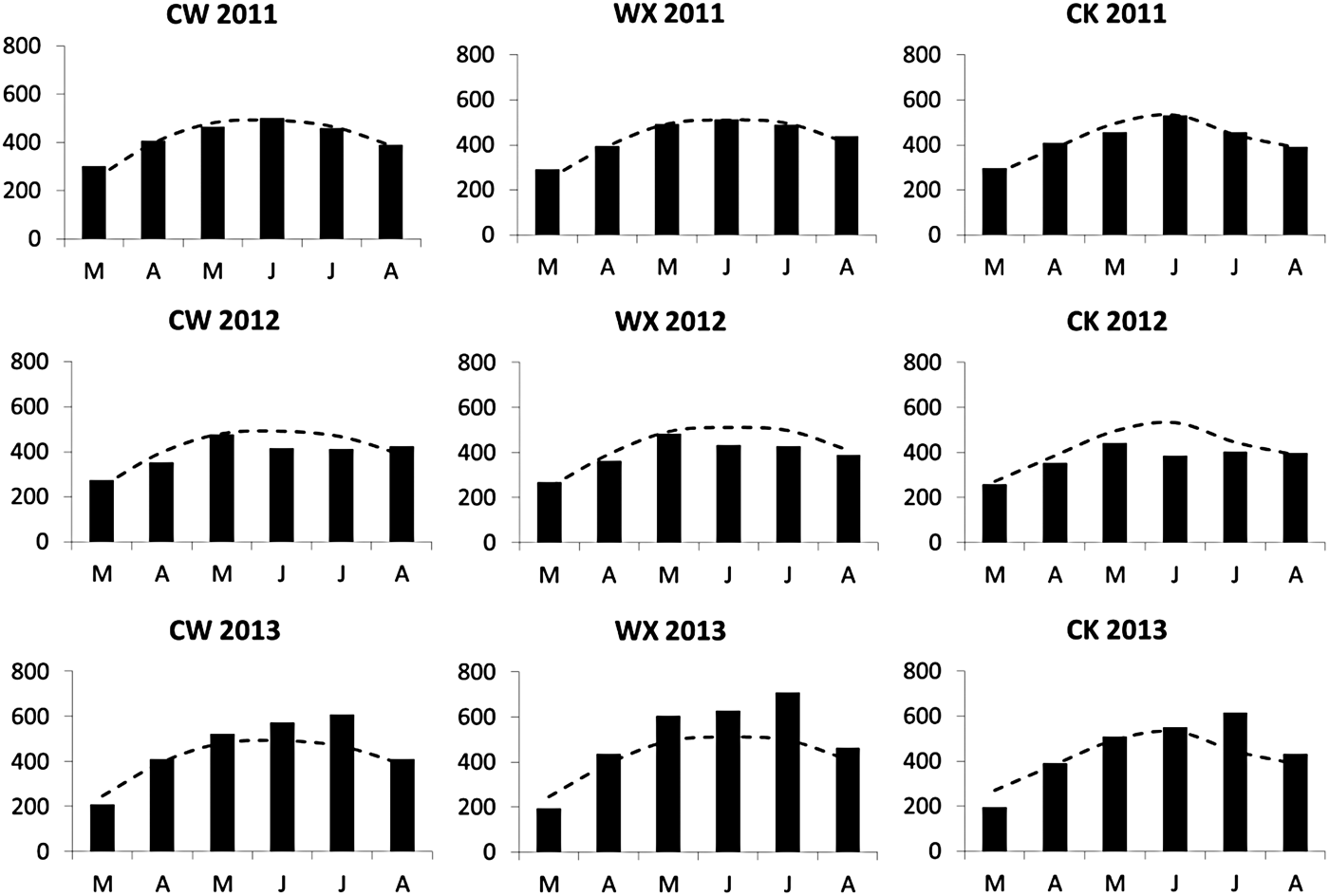
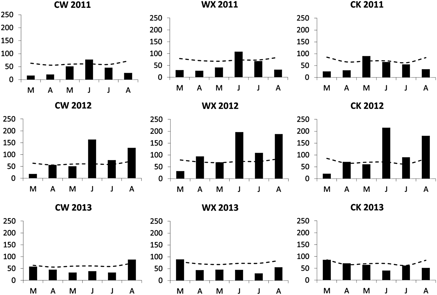
Temperature, solar radiation and rainfall data for each site/season along with average values throughout the spring barley growing season (March–August) are given in Figs 1–3. The 2011 season was warmer than average at the start and cooler than average towards the end. The opposite was true for 2013. Temperatures in 2012 were slightly warmer than average in March but comparable to or cooler than average for the other months. There was little difference between sites within a given season. The highest monthly accumulated solar radiation levels of the three seasons were in 2013. In 2011, solar radiation was close to and sometimes slightly above average, while in 2012 it was well below average, particularly in June and July. Again, there was relatively little difference in the pattern between sites in any given year except for WX 2013, which received slightly higher levels of solar radiation during the period May–July than the other two sites in that year. Accumulated monthly rainfall data tended to reflect the pattern of solar radiation where high rainfall levels accompanied low solar radiation levels and vice versa. There were very high levels of rainfall in the summer of 2012, particularly in June. The 2013 season had the wettest conditions immediately before and after plant emergence, while 2011 had the driest. However, in both cases, total rainfall values remained below or close to the long-term average across the entire growing season.
Monthly mean temperatures (°C) from March to August at all site/seasons. Associated long-term-average values (1981–2010) for each site are shown as a broken line.

Monthly accumulated solar radiation (MJ/m2) from March to August at all site/seasons. Associated long-term-average values (2005–2012 for CW and WX; 2008–2010 for CK) for each site are shown as a broken line.

Monthly accumulated rainfall (mm) from March to August at all site/seasons. Associated long-term-average values (1981–2010) for each site are shown as a broken line.

Yield and yield components
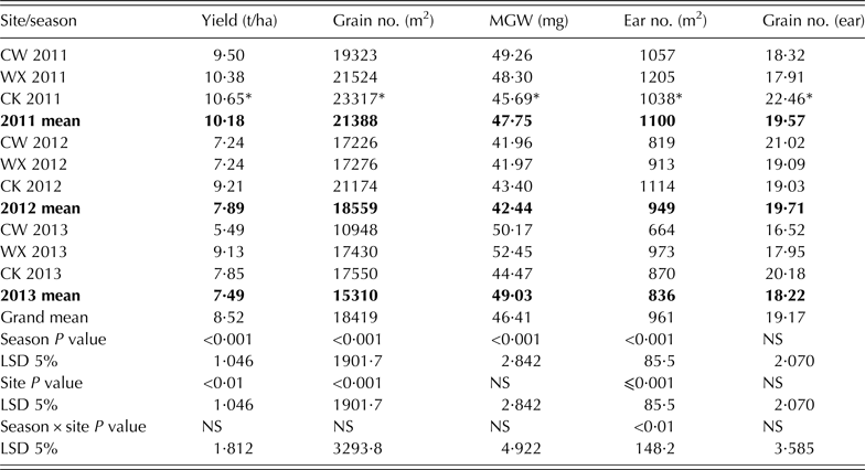
Yield and yield component values are given in Table 2. Higher yields were achieved in 2011 than in 2012 and 2013 (P < 0·001). There was a significant site effect on yield (P < 0·01), with CW achieving the lowest or joint lowest yields of the three sites in all three seasons and CK achieving the highest yield in two out of three seasons. A higher grain number/m2 was also achieved in 2011 than in 2012 and 2013 (P < 0·001), with CK consistently achieving the highest of the three sites followed by WX and CW (P < 0·001). Grain number/m2 at CW in 2013 was particularly low in comparison with other sites in that season. MGW in 2012 was lower than in 2011 and 2013 (P < 0·001). There was a significant season × site interaction effect on ear number/m2 (P < 0·01), where WX achieved the highest in 2011 and 2013 but not in 2012. As with grain number/m2, ear number/m2 at CW in 2013 was particularly low in comparison to other sites in that season.
Yield and yield components for all site/seasons. Season means in bold

P values and LSD at 5% for season, site, and season × site interaction effects are also given. Yield and mean grain weight (MGW) values are expressed at 85% dry matter.
NS, not significant.
* = CK harvest values estimated from combine threshed grain samples and/or previous growth analysis sample.
Lodging and ear blight
Lodging and brackling at harvest occurred only at WX and CK in 2013, but there was no severe lodging, i.e. flat (45°–90°) areas at either site. Plot scores of 0·70 and 0·47 for stem lodging (5°–45°) and 0·15 and 0·38 for brackling were recorded at WX and CK, respectively. As lodging occurred late in grain filling and was modest in terms of the angle of displacement (5°–10°), yield loss from lodging and brackling was expected to be minimal, especially from hand-harvested quadrats where collection of ears and grains was not compromised. In 2012, CW had higher levels of ear blight than WX and CK (P < 0·001). The fractions of ear area with symptoms of ear blight at CW, WX and CK in 2012 were 0·229, 0·104 and 0·086, respectively.
Crop growth, development and resource capture
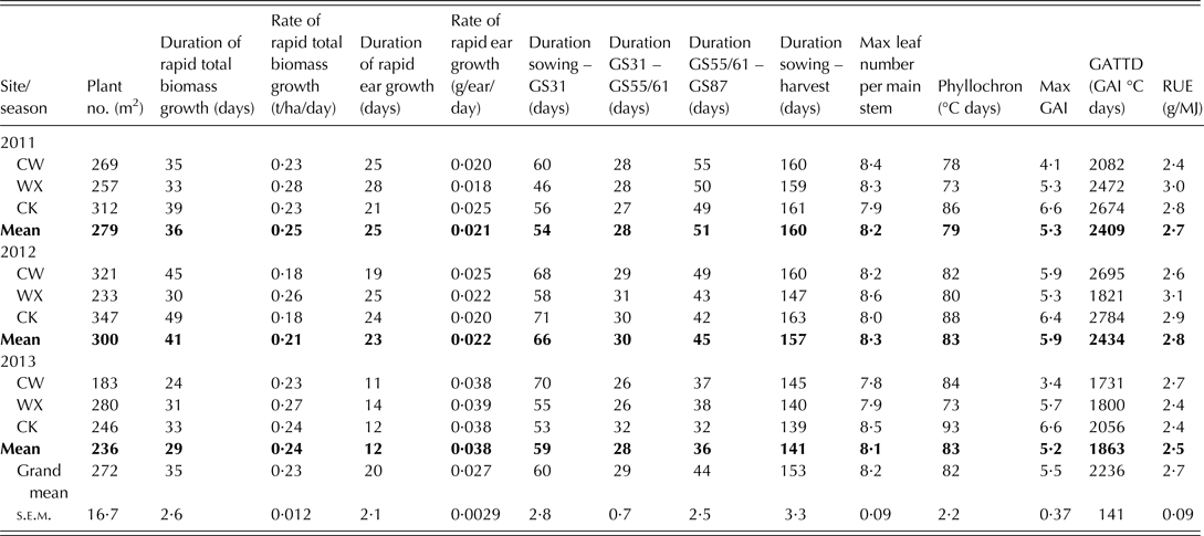
Crop development at the three sites followed a largely similar trend within seasons. Across all site/seasons, a range in sowing date of 25 days was reduced to a range in harvest date of 19 days. Table 3 shows a mean plant number/m2 of 272 was achieved across all site/seasons equating to an establishment rate of 0·78; plant establishment was lowest at CW in 2013.
Measures of growth, development and resource capture for all nine site/seasons

Season means in bold.
GAI, green area index; GATTD, green area thermal time duration post-anthesis; RUE, radiation use efficiency.
The mean leaf number per main stem achieved for the nine site/seasons was 8·2 (Table 3) with a significant site × season interaction effect (P < 0·05). The mean phyllochron for the nine site/seasons was estimated at 82 °C days (range 19·7) (Table 3). A grouped simple linear regression was performed on the leaf emergence and thermal time data using GenStat and this showed that slopes (the reciprocal of which was the phyllochron) did not differ significantly between sites, seasons and site/season combinations.
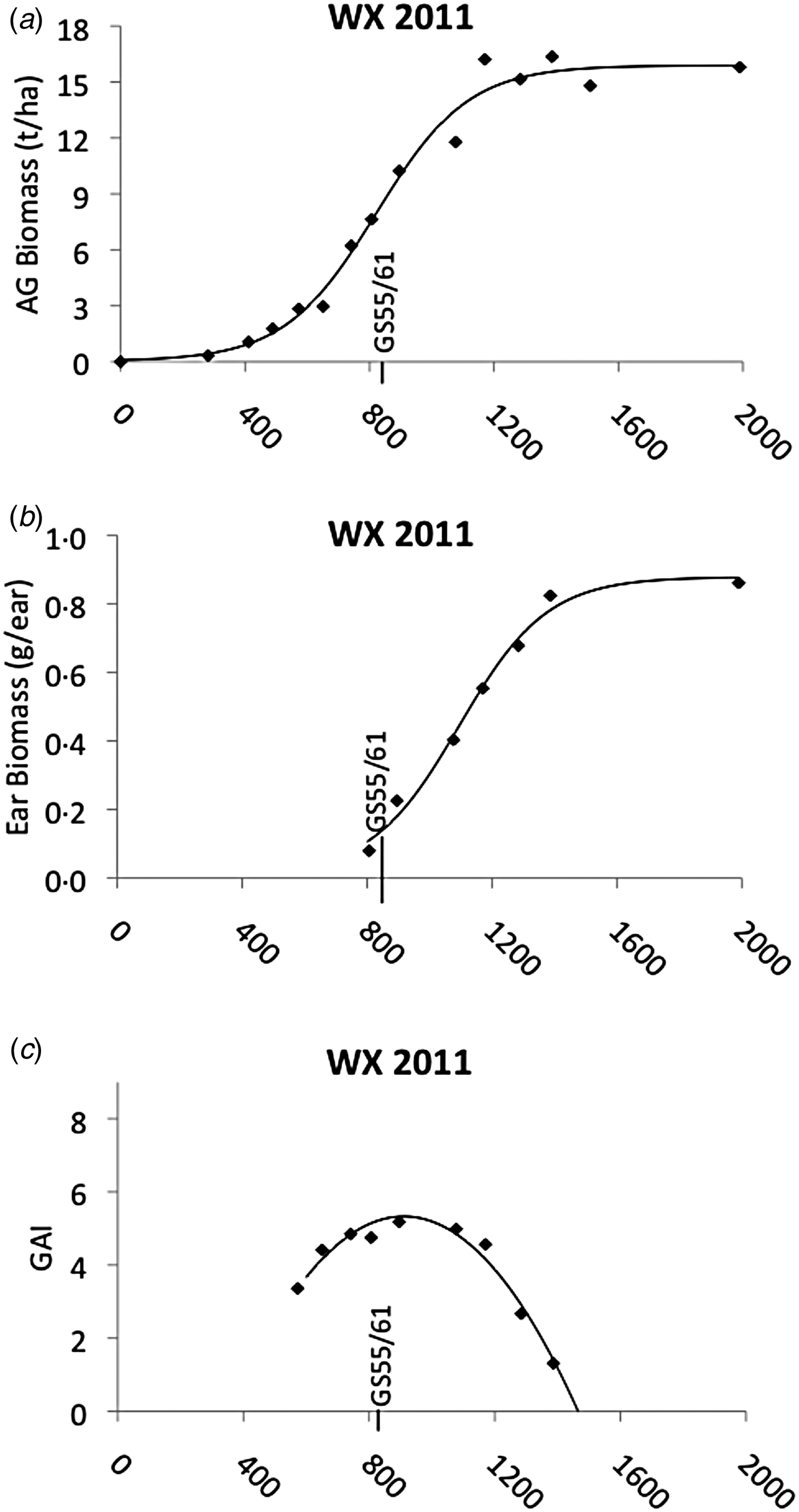
To investigate the variation in rates and duration of crop growth between site/seasons, logistic functions were fitted to plots of total above-ground biomass and ear biomass against thermal time from sowing (see Fig. 4, for example). The logistic regression model fitted the data well with R 2 values >0·95 for both variables at all site/seasons (P always < 0·001). The beginning and end points of the rapid linear growth phases were estimated. Total biomass growth accelerated around GS31 but began to slow down before total ear growth at all site seasons. There was on average a 14-day period between the estimated point at which total biomass growth slowed and ear growth slowed, meaning ear dry matter accumulation continued at a rapid rate as a result of re-partitioning of dry matter while total biomass accumulation began to slow down.
Seasonal growth at WX 2011 which was chosen as a representative example for all sites/seasons. Zadoks GS55/61 (50% ear emergence coincident with anthesis) is marked. Each point is the mean of three replicates for (a) total above ground (AG) biomass (t/ha at 100% dry matter), (b) ear biomass (g/ear at 100% dry matter) and (c) Green Area Index (GAI). All are plotted v. thermal time from sowing (°C days). Plots (a) and (b) are fitted with a logistic regression and (c) with a polynomial (second order) regression.

The estimated start of the period of rapid linear total biomass growth occurred on average 69 days (range 28) and 647 °C days (range 181) after sowing. The estimated start of the period of rapid grain growth occurred on average 11 days (range 18) and 138 °C days (range 248) after anthesis. Total biomass growth and grain growth continued beyond the end of the estimated rapid period but at lower rates. The estimated durations and rates of these linear phases of rapid growth are shown in Table 3. The entire cropping season (from sowing to harvest) lasted on average 153 days. It took on average 60 days from sowing for crops to reach the beginning of stem extension with the stem extension period itself lasting on average just 29 days. The post-anthesis period up to physiological maturity continued for 44 days.
Polynomial regressions (second order) fitted plots of thermal time v. GAI reasonably well with R 2 values >0·74 at all site/seasons (see Fig. 4, for example). The estimated max GAI occurred on average 62 °C days after ear emergence/anthesis. This is understandable as maximum GAI would not be expected to occur until the stem and in particular the peduncle completed extension after ear emergence. Maximum GAI ranged in value from 3·4 at CW 2013 to 6·6 at CK in 2011 and 2013. Post-anthesis GATTD ranged in value from 1731 GAI °C days at CW 2013 to 2784 GAI °C days at CK 2012 (Table 3). All sites except CW 2013 intercepted >0·93 of available PAR at anthesis. A value of just 0·70 was achieved at CW 2013, where canopy closure did not occur due to the poor and delayed crop establishment.
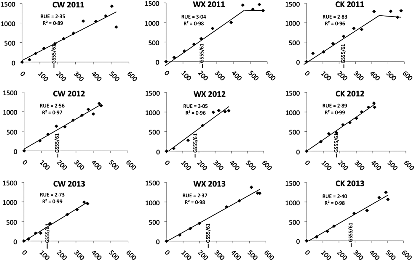
Significant non-linearity of RUE (i.e. slope of accumulated dry matter gain v. accumulated PARint), occurred at WX 2011 and CK 2011 (Fig. 5). At these two site/seasons a split line (two-line) regression accounted for more of the variation than a single line regression (R 2 values increased from 0·96 to 0·98 at WX 2011 and from 0·92 to 0·96 at CK 2011). The slope of the second line was not significantly different to zero, suggesting that RUE had levelled off. Here, maximum potential post-anthesis RUE was estimated as the slope of the first line, which covered the developmental period from stem extension (GS 31) to approximately early dough (GS 83) at the two sites. At all other site/seasons RUE was linear, where regression analysis gave R 2 values >0·89 and P always <0·001. Data are displayed in Fig. 5 and summary values given in Table 3. A grouped simple linear regression was performed on the intercepted PAR and accumulated dry matter gain data from the linear portions using GenStat and this showed that slopes (RUE) did not differ significantly between sites or seasons. However, there was a significant difference between site/season combinations (P < 0·05).
Regression analysis for plots of accumulated dry matter gain (g/m2) (y-axis) v. accumulated PAR intercepted (MJ/m2) (x-axis) at all site seasons from GS 31 to senescence. Radiation use efficiency (RUE, g/MJ) was estimated as the slope of the line. Split-line regression is shown for WX 2011 and CK 2011. GS55/61 (50% ear emergence coincident with anthesis) is marked.

When post-anthesis data points only were used to estimate post-anthesis RUE at all nine site/seasons, linear regression, while significant at each site/season, was statistically weaker than season-long estimates. A grouped simple linear regression was performed on the intercepted PAR and accumulated dry matter gain post-anthesis data using GenStat and this showed that slopes (RUE) did not differ significantly between sites, seasons and site/season combinations. The mean post-anthesis RUE was 2·23 g/MJ.
Determinants of yield
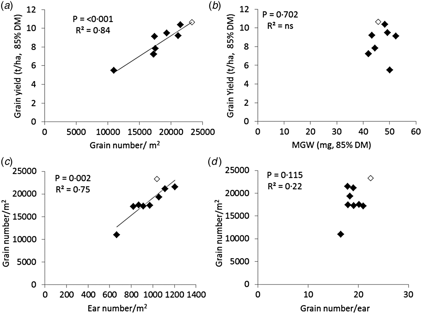
Of the two main yield components, grain number/m2 accounted for most of the variation in yield (P < 0·001, R 2 = 0·84), while MGW remained relatively less variable across sites and seasons (Fig. 6(a) and (b)). In turn, ear number/m2 accounted for most of the variation in grain number/m2 (P < 0·01, R 2 = 0·75), while grain number/ear remained relatively less variable across sites and seasons (Fig. 6(c) and (d)). There was no relationship between ear number/m2 and grain number/ear.
Linear regressions of (a) yield v. grain number/m2; (b) yield v. mean grain weight (MGW); (c) grain number/m2 v. ear number/m2 and (d) grain number/m2 v. grain number/ear. Hand-threshed data are used. Unfilled marker is the CK 2011 data point where values were estimated from combine threshed grain samples. DM = 100% dry matter.

Tillering dynamics
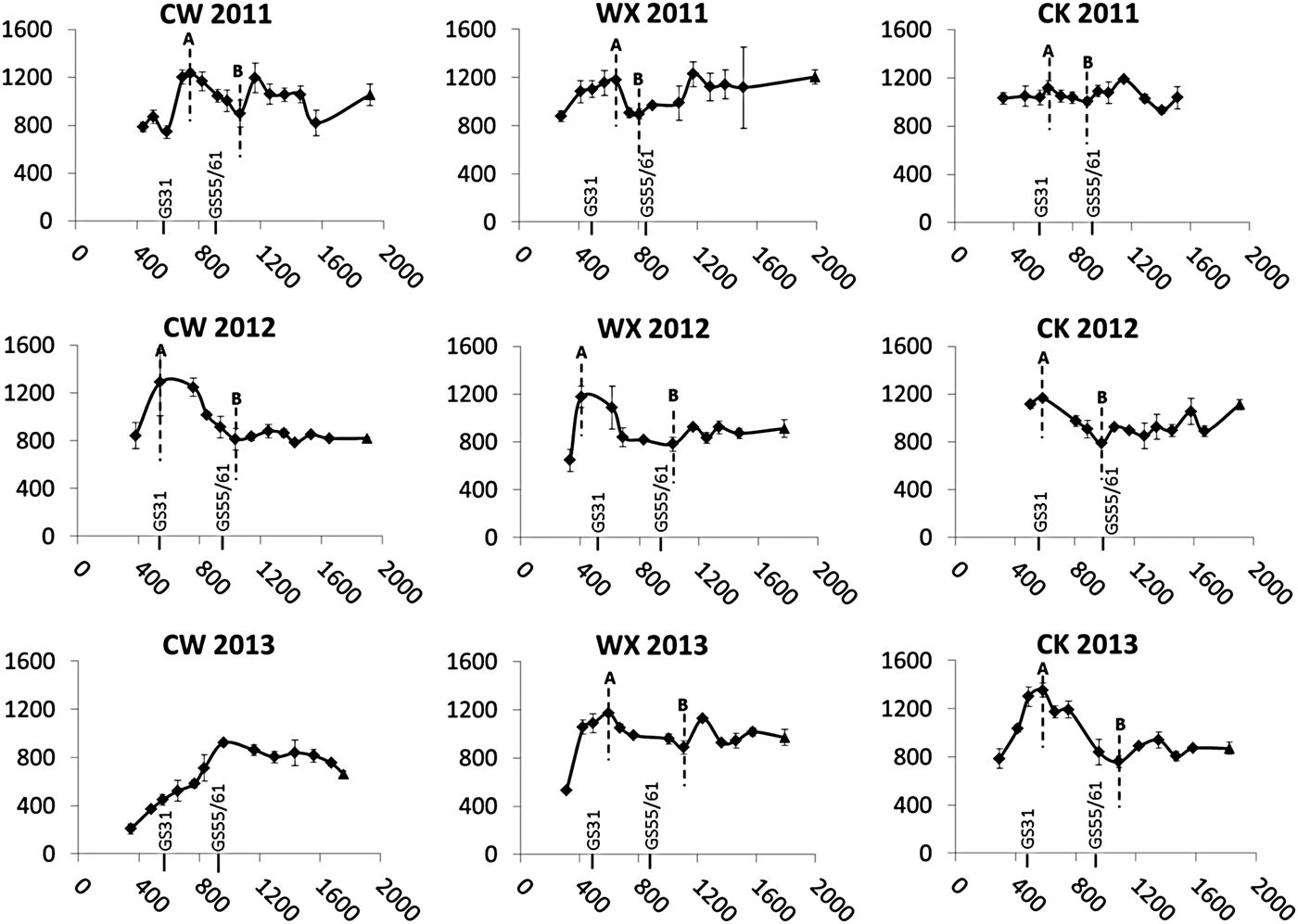
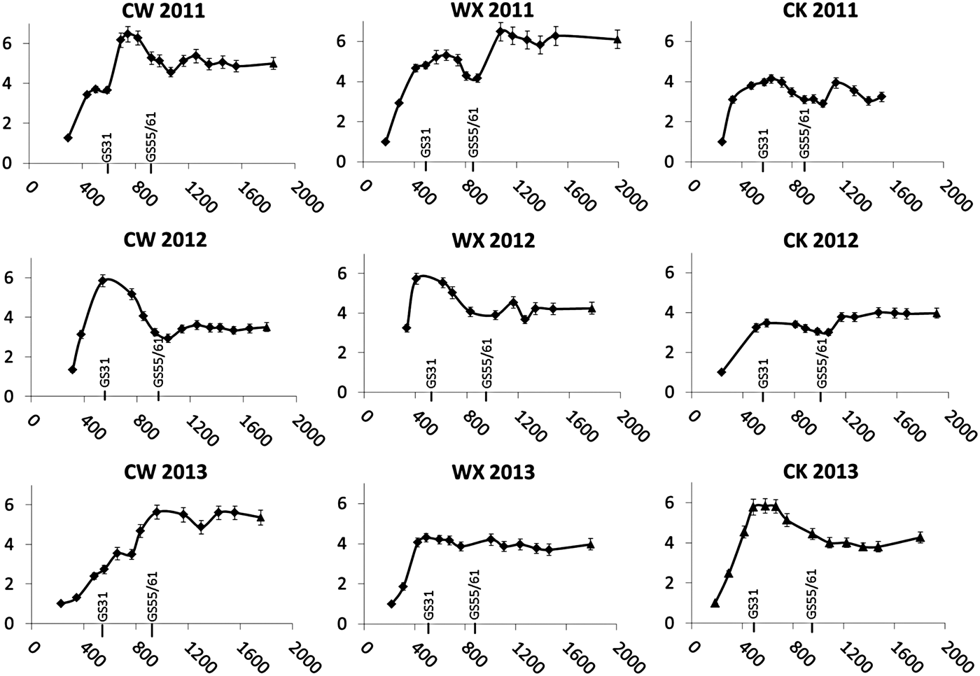
Shoot number/m2 plotted against thermal time for each site/season is shown in Fig. 7. The tillering pattern widely reported in the literature of maximum production at the beginning of stem extension (GS31), followed by a period of tiller death up to anthesis (GS55/61) then stabilization through to harvest was not clearly evident across all sites and seasons. An early-season maximum shoot number occurred at or around GS31 at six of the nine site/seasons, between GS31 and GS55/61 at two site/seasons and after flowering in one site in one season (CW 2013). A period of early–mid season shoot death was identified, which began during the stem extension period in all site/seasons except CW 2013 and continued until after flowering in five of the site/seasons. This period of shoot death was followed by some degree of post-anthesis re-tillering, which was itself followed by further death and apparent re-tillering at some site/seasons. The data presented in Fig. 7 were taken from quadrat samples. Quadrats represent a limited area of the plot whose location differs between different sampling dates. Variation in crop growth within the plot might contribute to variation in shoot numbers over time as illustrated by the relatively large error bars at some time points in Fig. 7. Revisiting and closely inspecting the same set of tagged plants weekly for shoot growth and death provided a potentially more accurate measure of tillering dynamics than bulk quadrat samples. Figure 8 shows a broadly similar tillering pattern for all site/seasons albeit in shoot number/plant format, to that shown in Fig. 7. There was also similar evidence of subsequent re-tillering post-anthesis. The largely similar patterns observed between Figs 7 and 8 provide confidence that the maxima and minima shoot number described above are real events resulting from tiller production, mortality and re-tillering, and are not a consequence of sampling error. Excluding CW 2013 because of its unusually low plant number and canopy size, the mean early-season maximum value at the start of the identified shoot death period was 1212 shoots/m2 (range 233), the mean mid-season minimum value was 854 shoots/m2 (range 250) and the mean harvest value was 999 shoots/m2 (range 386).
Shoot number/m2 data (y-axis) from quadrat samples for each site/season plotted against thermal time from sowing (x-axis). Vertical dashed lines indicate the period of early–mid season shoot death where A = early-season maximum shoot number/m2 and B = mid-season minimum shoot number/m2. Zadoks growth stages GS 31 (beginning of stem extension) and GS 55/61 (50% ear emergence taken to coincide with anthesis) are labelled. Error bars are ± one s.e. of the mean. Values include both ear-bearing and non-ear-bearing potentially fertile tillers except at harvest where only ear-bearing tillers were counted (▲). No harvest value available for CK 2011.

Shoot number/plant data (y-axis) from tagged plants for each site/season plotted against thermal time from sowing (x-axis). Zadoks growth stages GS 31 (beginning of stem extension) and GS 55/61 (50% ear emergence coincident with anthesis) are labelled. Error bars are + one s.e. of the mean. Values include both ear-bearing and non-ear-bearing potentially fertile tillers except at harvest where only ear-bearing tillers were counted (▲). No harvest value available for CK 2011.

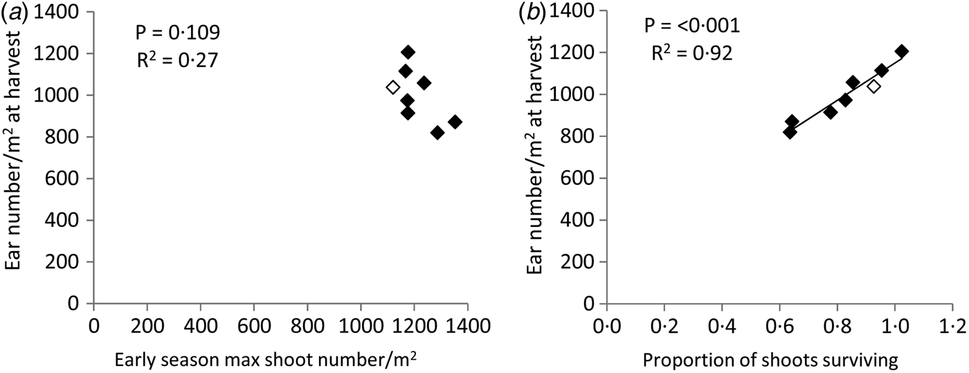
The results of regression analysis show that when CW 2013 data are excluded, an early-season maximum shoot number/m2 had no relationship with harvest ear number/m2 across sites and seasons (R 2 = 0·27, Fig. 9(a)). On the other hand, there was a strong positive association between the proportion of shoots surviving from this early season maximum through to harvest and harvest ear number/m2 (P < 0·001, R 2 = 0·92, Fig. 9(b)). However, as stated above, this shoot survival was a consequence of periods of both shoot death and re-tillering, which varied in duration and magnitude depending on site/season.
Plots of ear number/m2 at harvest v. (a) early-season maximum shoot number/m2 and (b) proportion of shoots surviving (early season maximum to harvest). Results of regression analysis are given. Data exclude CW 2013. Unfilled marker is the CK 2011 data point where the harvest ear number/m2 value was estimated from the previous growth analysis sample date.

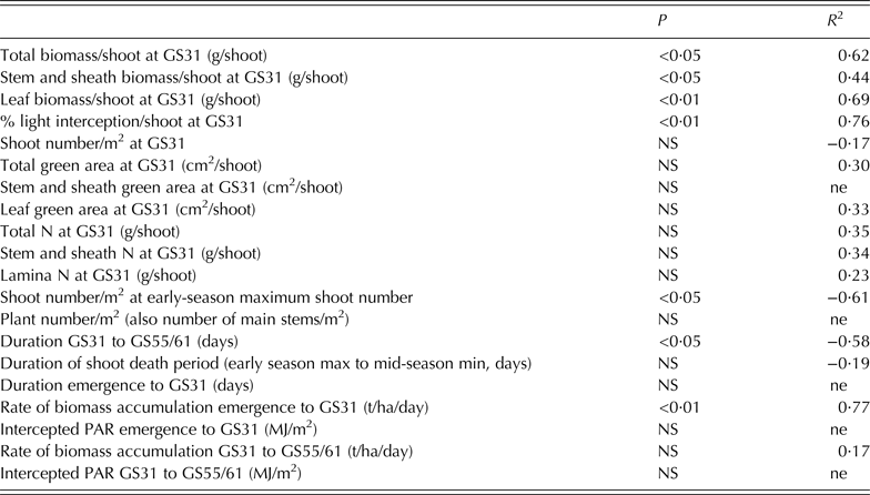
There was a statistically significant association between total biomass/shoot at GS31 and the proportion of shoots surviving during the identified shoot death period from an early-season maximum shoot number to a mid-season minimum shoot number (Table 4, P < 0·05, R 2 = 0·62). When this biomass was broken down into component plant fractions, the strongest relationship was between leaf biomass/shoot and shoot survival during this period (P < 0·01, R 2 = 0·69). There was also a similarly strong relationship with the proportion of light intercepted per shoot at GS31, but not with shoot number/m2 at GS31. There were weak but non-significant relationships between green area/shoot and shoot N content at GS31 and the proportion of shoots surviving. A negative relationship between shoot number/m2 at the early season maximum and shoot survival (P < 0·05, R 2 = 0·61) illustrates that where initial shoot production was high, a smaller proportion of them survived. Plant number/m2 which could be used as a proxy of the number of main stems at the time of early-season maximum shoot number had no relationship with shoot survival. The duration of stem extension (from GS31 to anthesis) was significantly and negatively associated with shoot survival (P < 0·05, R 2 = 0·58), i.e. the longer the duration of stem extension the smaller the proportion of shoots surviving. The duration of the shoot death period itself was not significantly associated with shoot survival (R 2 = 0·19); the same was true for the duration of the period from emergence to GS31. However there was a strong association between the rate of biomass accumulation from emergence to GS31 and shoot survival (P < 0·01, R 2 = 0·77). There was no significant association between the rate of biomass growth during stem extension (GS31 to anthesis) and shoot survival.
Regression analysis of the relationship between the proportions of shoots surviving (from the early-season maximum shoot number to the mid-season minimum shoot number) and a range of growth variables at GS31, early-season maximum shoot number, pre-GS31 and post-GS31

CW 2013 data excluded. A minus sign before the R 2 indicates the association was negative.
NS, not significant; ne, R 2 was not estimated because the residual variance exceeded the variance of the response variate.
There was no relationship between mid-season minimum shoot number/m2 (before re-tillering) and the harvest ear number/m2 (Fig. 10). Mean harvest values were higher than mid-season minimum values at all site/seasons except CW 2013 where potentially fertile shoot number decreased in the run up to harvest. There was a significant site × season × time interaction effect on shoot number/m2 (P < 0·05, LSD = 161·5) where harvest ear number/m2 was significantly higher than mid-season minimum shoot number/m2 at two sites (WX 2011 and CK 2012). Regression analysis (excluding CW 2013), showed that light interception at the mid-season minimum time-point was not related to the % shoot increase from the mid-season minimum to harvest. The same was true for values of accumulated rainfall for 1 and 2 weeks prior to the mid-season minimum.
Scatter plot of ear number/m2 at harvest v. mid-season minimum shoot number/m2 with a 1 : 1 line. Values are means of three replicates. Unfilled marker is the CK 2011 data point where the harvest ear number/m2 value was estimated from the previous growth analysis sample date. LSD 5% for the site × season × timing interaction effect obtained from ANOVA is also shown.

Realization of high yield potential
Linear regression analysis showed that there was no relationship between grain number/m2 and MGW for the nine site/seasons. Strong relationships were found between grain number/m2 and harvest ear biomass (P < 0·001, R 2 = 0·84), harvest total biomass (P < 0·001, R 2 = 0·92) and accumulated ear biomass post-anthesis (P < 0·002, R 2 = 0·74). The relationship between grain number/m2 and accumulated total biomass post-anthesis, while significant, was not as strong (P < 0·05, R 2 = 0·47). There was no significant relationship between grain number/m2 and stem biomass decline from anthesis to physiological maturity (GS55/61 to GS87). There were also no significant relationships between grain number/m2 and PARint post-anthesis and RUE post-anthesis.
DISCUSSION
Across nine site/seasons, the grand means achieved of 8·52 t/ha for yield, 18 419 for grain number/m2 and 46·41 mg for MGW were close to those of similar work in the UK on winter barley where grand means of 8·8 t/ha for yield, 18 600 for grain number/m2 and 46 mg for MGW were achieved across 18 site/seasons (Blake et al. Reference Blake, Bingham, Foulkes and Spink2006). Given that spring barley in any given environment can yield about 0·8 that of winter barley, the yield and yield component values achieved in the present study illustrate the high yield potential of barley in the Irish climate.
Grain number/m2 was strongly related to yield across sites and seasons, supporting previous findings in the literature across a range of environments (Gallagher et al. Reference Gallagher, Biscoe and Scott1975; Abeledo et al. Reference Abeledo, Calderini and Slafer2003; Blake et al. Reference Blake, Bingham, Foulkes and Spink2006; Bingham et al. Reference Bingham, Blake, Foulkes and Spink2007a ; Peltonen-Sainio et al. Reference Peltonen-Sainio, Kangas, Salo and Jauhiainen2007; Serrago et al. Reference Serrago, Alzueta, Savin and Slafer2013). This is evidence supporting the hypothesis that grain number/m2 determined yield, even in a high-yield potential temperate maritime climate.
Various source:sink manipulation experiments across a range of environments on barley (Willey & Holliday Reference Willey and Holliday1971; Habgood & Uddin Reference Habgood and Uddin1983; Grashoff & dAntuono Reference Grashoff and dAntuono1997; Arisnabarreta & Miralles Reference Arisnabarreta and Miralles2008b ), wheat (Fischer Reference Fischer1985; Abbate et al. Reference Abbate, Andrade, Culot and Bindraban1997) and triticale (Estrada-Campuzano et al. Reference Estrada-Campuzano, Miralles and Slafer2008) have highlighted the importance of the stem extension period for grain number determination through its influence on grain number survival. The above authors highlight the influence of grain number/ear rather than ear number/m2 on grain number formation during this period, and other theoretical discussions on yield improvement in wheat concur with this (Reynolds et al. Reference Reynolds, van Ginkel and Ribaut2000; Miralles & Slafer Reference Miralles and Slafer2007). However, in the present study, ear number/m2 at harvest was strongly associated with grain number/m2 and ear number itself was strongly associated with the proportion of shoots surviving from an early season maximum through to harvest. Grain number/ear accounted for little of the variation, thus supporting the hypothesis that grain number/m2 is most readily influenced by ear number/m2. The divergence from the literature on wheat is not surprising given that grain number/ear is relatively less variable in barley than in wheat. In wheat grain, number per ear is a function of both the number of spikelets per ear and the number of grains per spikelet, whereas in barley only one grain is produced per spikelet. However, the contrast in findings of the present study from the barley literature quoted above is surprising given that the literature cited relates almost exclusively to two-row barley similar in type to cvar Quench used in the present study. Also, where comparable data were presented in the literature (Willey & Holliday Reference Willey and Holliday1971; Grashoff & dAntuono Reference Grashoff and dAntuono1997), mean harvest ear number/m2 values for control treatments (~600–800) were lower than the present study mean of 961. The tillering pattern of barley can result in a maximum shoot number around the beginning of stem extension (GS31) followed by death during stem extension then stabilization from anthesis through to harvest (Gallagher et al. Reference Gallagher, Biscoe and Scott1975; del Moral et al. Reference del Moral, Ramos and Recalde1984; Slafer et al. Reference Slafer, Kantolic, Appendino, Miralles, Savin, Sadras and Calderini2009). While early season shoot number maxima followed by periods of shoot mortality were identified at all site/seasons, the maxima occurred at or around GS31 at only six site/seasons. At the other site/seasons this maximum occurred later, particularly so at CW 2013 where canopy closure did not occur due to poor plant establishment and as such maximum shoot number was not reached until after anthesis. For this reason, CW 2013 data points were excluded from various regression analyses investigating tillering dynamics. With CW 2013 excluded, the shoot mortality period began pre-anthesis at all sites/seasons but was not completed until after anthesis in five site/seasons. It is clear that the period of tiller production in barley is quite variable (Willey & Holliday Reference Willey and Holliday1971; Simmons et al. Reference Simmons, Rasmussen and Wiersma1982). It is also clear that the period of tiller senescence is similarly variable and is not always completed before anthesis. This is in agreement with some published literatures on wheat and barley (Lauer & Simmons Reference Lauer and Simmons1989; Sparkes et al. Reference Sparkes, Holme and Gaju2006).
At site/seasons in the present study where the early-season maximum shoot number was high, there was lower shoot survival. The early-season maximum shoot number/m2 itself had no relationship with ear number/m2 at harvest or yield. Variation in ear number/m2 at harvest was almost completely explained by variation in shoot survival from the early-season maximum through to harvest. Tiller mortality can vary with cultivar and environment (Thorne Reference Thorne1962; Kirby & Riggs Reference Kirby and Riggs1978; Simmons et al. Reference Simmons, Rasmussen and Wiersma1982) and survival rates of 0·68–0·37 (proportion of the maximum shoot number that survive to harvest) have been recorded in field studies of several cultivars and types of barley in contrasting Mediterranean environments (del Moral & del Moral Reference del Moral and del Moral1995). With CW 2013 excluded (because it did not reach maximum shoot number until post-anthesis), a mean shoot survival figure of 0·71 was achieved across the remaining eight site/seasons. This is at or above the higher end of the range set out by del Moral & del Moral (Reference del Moral and del Moral1995). However, the proportion of shoots surviving to form ears at harvest was the net effect of early–mid season shoot death and post-anthesis re-tillering. There was no relationship between the mid-season minimum shoot number and final ear number at harvest indicating that late tillering did make an appreciable contribution to final ear number at some sites. The contribution of these late developing tillers to yield cannot be quantified as measurements were not made on individual shoots or shoots of defined size category. However, the mid-season minimum shoot number (around anthesis) explained almost as much of the total variation in yield (P < 0·05, R 2 = 0·61) as final ear number (P < 0·01, R 2 = 0·66) (with CW 2013 excluded), suggesting that the later tillers contributed relatively little to yield. Moreover, there was a strong association between yield and the proportion of shoots surviving from the maximum number to the mid-season minimum (P < 0·05, R 2 = 0·62), indicating that shoot survival during this phase of tiller dynamics was important in determining yield. As such, the mechanisms controlling shoot death from the early season maxima to the mid-season minima warranted further investigation.
Measures of shoot biomass and size at GS 31, in particular the leaf portion of the shoots, had a greater influence on the proportion of shoots surviving from the early season maxima to the mid-season minima than measures of growth during stem extension. Crops that intercepted more light per shoot at GS 31 had greater shoot survival and this was not simply due to crops with fewer shoots/m2 having more assimilate available per shoot during stem extension, as there was no relationship between shoot number/m2 at GS 31 and shoot survival. A strong relationship between the rate of biomass accumulation from emergence to GS 31 indicates that factors contributing to individual shoot size, mass and ability to independently produce assimilates at GS 31 were most likely to influence shoot survival. The lack of relationship between plant population and shoot survival indicates that shoot survival was not proportionate to the number of main stems present.
A flush of late season tillering in response to a rainfall event is possible (Kirby Reference Kirby1967) particularly following a period of drought (Jamieson et al. Reference Jamieson, Martin, Francis and Wilson1995). It was difficult to test this hypothesis in the present study due to the absence of soil moisture data, however, accumulated rainfall in the week and 2 weeks prior to re-tillering events did not explain the variation in the increase in shoot number from mid-season minimum to harvest; neither did solar radiation availability low in the canopy following a possible thinning effect of shoot death.
Strong relationships between grain number/m2 and harvest ear biomass, harvest total biomass and accumulated ear biomass post-anthesis are not surprising given the strong relationship between grain number/m2 and yield – high grain number/m2 crops realized their high yield potential. The source of dry matter for filling grains in crops of large grain number/m2 is unclear. There was no relationship between grain number across site/seasons and either PARint post-anthesis, RUE post-anthesis or the decline in stem biomass from GS55/61 to GS87 (remobilization of dry matter). Therefore, it would appear that the relative contribution of each of the three variables differs across sites and seasons. This suggests that when the demand for assimilates for grain filling is increased by increasing grain numbers, there are multiple ‘routes’ by which the additional demand might be met. Experiments in which light availability is varied post-anthesis to crops of differing grain number might reveal the extent to which RUE and remobilization of soluble carbohydrate reserves can be adjusted to meet the demands for grain filling.
Radiation use efficiency declined or ‘levelled off’ late season in two out of nine site/seasons (WX 2011 and CK 2011). At these two site/seasons, green tissue continued to intercept radiation towards the end of grain filling but crops accumulated less dry matter per unit of intercepted radiation than they did earlier. Stem biomass decline began around the same time that RUE levelled off and grain growth was not completed until approximately 2–3 weeks later. Sources other than direct photosynthesis, such as remobilization of stored stem carbohydrate reserves may have sustained grain growth (Yoshida Reference Yoshida1972; Beed et al. Reference Beed, Paveley and Sylvester-Bradley2007; Foulkes et al. Reference Foulkes, Sylvester-Bradley, Weightman and Snape2007; Bingham & Topp Reference Bingham and Topp2009; Fabian et al. Reference Fabian, Jager, Rakszegi and Barnabas2011; Serrago et al. Reference Serrago, Alzueta, Savin and Slafer2013). Total biomass growth began to slow down before total ear growth at all site/seasons and this could be interpreted as further evidence of utilization of remobilized stored carbohydrate reserves for grain filling, but does not explain the decline in RUE at WX 2011 and CK 2011. An increase in respiration relative to photosynthetic activity with senescence (Bingham et al. Reference Bingham, Blake, Foulkes and Spink2007a ) or a decline in photosynthetic efficiency with leaf age (Biscoe et al. Reference Biscoe, Scott and Monteith1975) may be responsible. There may also exist a feedback control mechanism whereby photosynthetic activity is down-regulated due to a limited sink demand (Bingham et al. Reference Bingham, Blake, Foulkes and Spink2007a ), thereby reducing RUE below its potential (Newton et al. Reference Newton, Flavell, George, Leat, Mullholland, Ramsay, Revoredo-Giha, Russell, Steffenson, Swanston, Thomas, Waugh, White and Bingham2011). It is interesting to note that the decline in RUE was observed at the two sites with the greatest yields. Both WX 2011 and CK 2011 had significantly higher grain number/m2 than the other site in that season, CW 2011, where RUE did not ‘level-off’ post-anthesis. In fact, WX 2011 and CK 2011 had the highest and second highest grain numbers/m2 of all nine site/seasons. It is unlikely, therefore, that if a limited sink demand was responsible for the down-regulation of photosynthesis that it was due to a limited grain number/m2. However, sink capacity is a function of both the number of grains produced and their individual storage capacity. Thus, a limited sink demand in the form of a limited grain storage capacity may have occurred, where the ability of the grain to accumulate dry matter was restricted (Bingham et al. Reference Bingham, Blake, Foulkes and Spink2007b ). The fact that grain weights at WX 2011 and CK 2011 were lower than at CW 2011 (although not significant at WX 2011) could be an indication that at very high grain numbers, individual grain storage capacity is a sink-limitation to yield in barley. Although no relationship was found between grain number/m2 and MGW across sites and seasons, it is conceivable that within a given environment attempts to raise the yield potential by increasing grain number through agronomy or breeding might be eventually offset by restrictions on grain storage capacity and MGW. A better understanding is required of the mechanisms controlling grain storage capacity and its interaction with grain number and resource availability post-anthesis.
In conclusion, Ireland has a high yield potential for spring barley. In such a high-yielding environment where large numbers of grains are produced, it is conceivable that there may be less assimilate available per grain for grain filling and that yield may become source-limited more frequently. However, the results show that grain number of spring-sown barley was strongly associated with yield and thus even in high-yield potential climates, yield appears to be predominantly sink-limited. Survival of potential grain sites had a strong influence on harvest grain number, but in contrast to the literature it was the survival of ears rather than grains/ear that was of greater importance. Therefore, the hypothesis that grain number of high-yielding two-row spring barley crops is more strongly associated with ear number can be accepted. The period over which ear number was determined was more flexible than the literature suggested. Yield was strongly associated with shoot survival from an early season maximum through to a mid-season minimum reached around or after anthesis. Shoot size and weight at GS31 had the largest influence on shoot survival, indicating that crop condition at GS31 and hence growth and development pre-GS31 may be more important for shoot survival than growth and development during the stem extension period. Achieving high shoot numbers of adequate size and weight at GS31 may be an appropriate target for establishing a high-yield potential crop. Optimizing seeding rates and seedbed conditions to ensure rapid plant establishment and early vegetative growth, along with good crop husbandry to eliminate pest, disease and weed competition during the pre-GS31 period should result in crops of sufficient shoot number at GS31. The agronomic effort to ensure that these shoots are of adequate size and weight will also involve eliminating macro- and micro-nutrient deficiencies during the same period.
We thank the technical staff of Teagasc Oak Park for assistance with the field experiments. This study was funded by Teagasc – The Irish Agriculture and Food Development Authority and Shane Kennedy was supported by the Teagasc Walsh Fellowship programme. SRUC receives financial support from the Scottish Government's Rural and Environment Science and Analytical Services (RESAS) division.