1. Introduction
After 25 years of relatively mild business cycle fluctuations in the USA, the so-called “Great Moderation,” the Great Financial Crisis (GFC) caused tremendous turmoil and drew the US economy into the Great Recession of 2009. In the business cycle literature, the Great Moderation (see, among others, Stock and Watson (Reference Stock and Watson2002), Gali and Monacelli (Reference Gali and Monacelli2005), and Giannone et al. (Reference Giannone, Lenza and Reichlin2008)) was one of the most studied phenomena until the Great Recession shifted researchers’ focus (see, among many others Christiano et al. (Reference Christiano, Eichenbaum and Trabandt2015), Mian and Sufi (Reference Mian and Sufi2010), Aiyar (Reference Aiyar2012)). However, the relationship between the two has been neglected by most of the literature. This paper argues that the Great Moderation and Great Recession are essentially the same phenomenon—two sides of the same coin—and that the financial cycle is the force that forged it.
This approach is motivated by the observation in Figure 1. This figure shows that the financial cycle—represented by credit-volume-to-GDP (the so-called “credit gap”) and house prices—witnessed large gains in its amplitude precisely at the same time that the business cycle began its moderation. An increase of financial market volatility thus occurred long before the housing market bubble that eventually led to the GFC even began to build up. I find a single Granger-causal empirical relationship between the credit gap and output that rationalizes this observation. This relationship is such that credit can attenuate short-term output fluctuations and amplify medium-term output fluctuations. This led to two “shifts” that give the Great Moderation a new narrative: a shift of output volatility toward longer-term fluctuations, as shown before in Crowley and Hallett (Reference Crowley and Hallett2015), and a shift in the source of medium-term volatility from the real (non-financial) to the financial sector. These shifts are both independent of the Great Recession.
Business cycle (GDP) and financial cycle (Indicator) in the USA.
Note: This figure shows the evolution of the US business cycle and financial cycle between 1970 and 2018. The business cycle is calculated as the fluctuations between 5 and 32 quarters of GDP around its trend. The financial cycle is an indicator routinely calculated by the Bank for International Settlements as the average of the cyclical components of total credit volume, credit gap, and house prices. The cyclical components are extracted with a bandpass filter with bounds of 32 and 120 quarters.

The main contribution of this paper is the empirical characterization of the relationship between the business cycle and the financial cycle over the last five decades. Therefore, I use spectral analysis to decompose business cycle fluctuations into volatilities of different periodicities. Then, I estimate vector-autoregressive models (VARs) that describe the relationship between output and financial variables. In this context, I show how to use frequency-domain techniques to evaluate the properties of the VAR models and obtain novel results. Specifically, I characterize Granger-causal relationships between the financial cycle variables, credit gap and house prices, and output (GDP). Finally, I identify structural shocks from the estimated VAR models to assess which shocks drive fluctuations of different periodicities. With this approach, I find that the volatility of the post-1984 economy moved mainly outside the classic business cycle range of cycles of 5–32 quarters (Burns and Mitchell (Reference Burns and Mitchell1946)) onto medium-term fluctuations between 32 and 120 quarters. While this led to a reduction in short-term volatility, medium-term volatility increased. This shift came with a shift in the origin of output volatility from the real (non-financial) sector to the financial sector: I show that shocks to financial variables increase greatly in importance, but systematically drive mainly medium-term output volatility in the Great Moderation economy. Meanwhile, real shocks (such as TFP shocks) continue to drive the majority of short-term output volatility.
Jointly, these shifts imply that the defining feature of the Great Moderation was a finance-driven shift in the origin of output volatility and the distribution of output volatility across fluctuations of different lengths. These changes of the Great Moderation are linked by a Granger-causal relationship between credit gap and output, which is not uniform across fluctuations of different lengths. Short-cycle reductions in output lead to short-cycle expansions of the credit gap. At the same time, medium-cycle expansions (contractions) in the credit gap lead to medium-cycle expansions (contractions) of output. In other words, short-cycle credit gap movements attenuate short-cycle output movements, while medium-term credit gap movements amplify medium-term output movements. The short-term fluctuations for which I find the attenuation forces of credit are precisely the same on which I find that a moderation of output volatility occurred. At the same time, the fluctuations in which financial shocks manifest themselves as volatility are those on which the amplification forces and the resulting increases in output volatility are found.
I show that the attenuation-amplification property of the relationship between the credit gap and output is not an artifact of the Great Moderation or the Great Recession period, but can be found in multiple periods of the US economy after World War II. I argue that, by this relationship, the Great Moderation and the Great Recession are the consequences of the attenuation and amplification forces, respectively. Therefore, they are inextricably linked.
The secondary contribution is the construction of a model that can replicate the most important frequency-domain features of the data. I show that a combination of modeling elements is required for this: a collateral constraint on an entrepreneur, as in Iacoviello (Reference Iacoviello2005) that gives rise to a financial accelerator, a leverage constraint on the financial intermediary, as in Gertler and Karadi (Reference Gertler and Karadi2011) and the presence of long-run risk, borrowed from Bansal and Yaron (Reference Bansal and Yaron2004) on the cost of entrepreneurial investments and the lending ability of the financial intermediary. The collateral and leverage constraints generate the necessary interaction between the financial sector and the real sector. The long-run risk generates the necessary persistence to explain the medium-term fluctuations and ensures that shocks to the investment cost systematically feed into medium-term output volatility. In the absence of any of those three elements, the model’s moments do not come close to those of the data. This extends to many standard off-the-shelf models from the literature, which consistently fail to reproduce the non-uniformity of the effects of financial and non-financial shocks on fluctuations of different lengths.Footnote 1
The long-run risk is the theoretical counterpart to the argument that the Great Moderation and the Great Recession are two sides of the same coin. The presence of this risk has effects on prices in phases of moderate volatility, but its main effect is only observed in relatively rare but consequential events. I then use the parameter estimates of the model to refine the “good luck” hypothesis of the Great Moderation by showing that only the standard deviation of non-persistent (short-run) shocks moderated, while very persistent (long-run) shocks witnessed increases in their standard deviations. Additionally, I isolate the changes due to monetary policy that occurred during the Great Moderation. I show that while monetary policy in the Great Moderation reduced short-term output volatility, it contributed to the systematic way that financial shocks cause medium-run output volatility. Therefore, it came at the expense of more medium-term volatility. In other words, I can use the model to refine the “good policy” hypothesis of the Great Moderation as well.
In the course of this paper, there are several instances where the frequency-domain approach is required in order to discover new insights into the economics of the business cycle and financial cycle. It reveals the non-uniformity of the empirical relationship between credit gap and output. Additionally, it leads to the finding that financial shocks systematically drive medium-term volatility. This adds a new property that economic models should be able to replicate.
The remainder of this paper is structured as follows: In Section 2 I discuss the relation of my paper to the existing literature. Section 3 presents the empirical case. Section 4 introduces the model and discusses its estimation. Section 5 analyzes the performance of the model on the frequency-domain properties of the time series, as well as two policy counterfactuals. Section 6 concludes.
2. Related literature
The paper is related to the literature in three ways: First, it is connected to the literature that characterizes the empirical properties of (domestic) financial cycles and their relationship with business cycles (see, for instance, Borio and White (Reference Borio and White2004), Borio et al. (Reference Borio, Drehmann and Xia2018), Claessens et al. (Reference Claessens, Kose and Terrones2011), Strohsal et al. (Reference Strohsal, Proaño and Wolters2019), Schularick and Taylor (Reference Schularick and Taylor2012), Verona (Reference Verona2016), or Drehmann et al. (Reference Drehmann, Borio and Tsatsaronis2012)). Especially noteworthy is the work by Jorda et al.`(Reference Jordà, Schularick and Taylor2010) who provide very long-run data on financial cycles. The main results of this literature are that 1) the financial cycle is significantly longer than the business cycle, 2) business cycle recessions that coincide with financial cycle downturns are larger and longer than those that do not, and 3) the financial cycle is aligned with medium-term business cycle fluctuations. These results are reflected in the findings of this paper. The prevalent approach of the literature has usually been to isolate fluctuations of a certain periodicity range with a band-pass filter and calculate the average effect over the periodicity window (see, for instance, Drehmann et al. (Reference Drehmann, Borio and Tsatsaronis2012) and Pancrazi (Reference Pancrazi2015)). The former use this technique to find a positive correlation of medium-term output fluctuations and the (BIS) financial cycle indicatorFootnote 2 . I advance this result by showing that the relationships between credit gap, house prices, and output are nonuniform across different periodicities. The frequency-domain approach of this paper allows me to calculate a profile of correlations associated with different periodicities and give a Granger-causal interpretation to them. The combination of the two yields a more detailed characterization of the empirical forces compared to the literature. In the case of credit gap and output, this yields a negative dynamic correlation on short periodicities in which output is Granger-causal and a positive dynamic correlation in which credit gap is Granger-causal on medium periodicities.
It has been recognized that credit booms sow the seeds of credit crunches (Minsky (Reference Minsky1986), Schularick and Taylor (Reference Schularick and Taylor2012), Aikman et al. (Reference Aikman, Haldane and Nelson2015)). Therefore, the relationship between financial variables and output has been used to explain the Great Recession (Gorton and Ordonez (Reference Gorton and Ordonez2020)Footnote 3 , Bean (Reference Bean2010), Jorda et al. (Reference Jordà, Schularick and Taylor2013)) or the failure to predict it (Gadea Rivas et al. (Reference Gadea, Dolores, Gómez-Loscos and Perez-Quiros2014)) and it has been shown that the pair of credit and asset prices is one of the most powerful early warning indicators of a recession (Aldasoro et al. (Reference Aldasoro, Borio and Drehmann2018)). However, this analysis is usually focused on the build-up of credit that occurred during the 2000s—not on the entire Great Moderation. This paper shows that the underlying relationship between credit and output that drives credit booms and busts, as well as phases of moderation and phases of high volatility, already existed long before the Great Recession and even before the Great Moderation. Instead, the relationship has intensified: Granger-causality from the financial to the non-financial sector has become more significant, and financial shocks cause more output volatility.
Second, these findings allow me to complement the existing views of the literature on the Great Moderation, which Crowley and Hallett (Reference Crowley and Hallett2015) and Pancrazi (Reference Pancrazi2015) recognized to have been very heterogeneous: The debate between the “good luck” hypothesis (see Stock and Watson (Reference Stock and Watson2003) and Ahmed et al. (Reference Ahmed, Levin and Wilson2004)) and the “good policy” hypothesis (Bernanke (Reference Bernanke2004) Footnote 4 , Boivin and Giannoni (Reference Boivin and Giannoni2006), and Benati and Surico (Reference Benati and Surico2009)), along with the competing explanation of increased asset market participation and the overall expansion of the US financial sector (Bilbiie and Straub (Reference Bilbiie and Straub2013) and Carvalho and Gabaix (Reference Carvalho and Gabaix2013)) centers on the initial causes of the observed reduction in short-term volatility during the early stages of the Great Moderation. Additionally, Crowley and Hallett (Reference Crowley and Hallett2018) recognizes elongation of the business cycle and the associated transfer of volatility to longer cycles may have been a side-effect of monetary policy. In the same spirit, Drehmann et al. (Reference Drehmann, Borio and Tsatsaronis2012) warn that monetary policy that does not take into account credit growth could dampen short-term volatility at the expense of more medium-term volatility, which implicitly questions how “good” the revised monetary policy was. The results of this paper do not stand in contrast to these positions, but I argue that none of these explanations are at the core of the changes that occurred during the Great Moderation, and I remain largely agnostic regarding what caused the upswing in credit gap. Instead, I emphasize that the increased amplitude over the duration of the cycle led to the Great Moderation. In this regard, I sharpen the finding of an increased contribution of the financial sector to output volatility in the Great Moderation by showing that financial shocks systematically feed into medium-term volatility. I also show that monetary policy contributed to the shift to higher volatility on longer cycles and confirm Drehmann et al. (Reference Drehmann, Borio and Tsatsaronis2012) position that the lack of monetary reaction to credit growth partially causes this shift.
3. Empirical case
This section first introduces the data and explains the methodological approach. Then, I show the shift of output volatility toward longer-term fluctuations that defines the Great Moderation. Further, I document the intensifying relationship of attenuation and amplification between credit gap and output, by characterizing co-movement and Granger-causality between these variables in the course of the Great Moderation. Finally, a structural interpretation shows how shocks on financial markets systematically cause medium-term output volatility in the Great Moderation economy.
3.1. Data
To study the interactions of real and financial markets, I focus on GDP as the most common measure of aggregate activity, while credit volume and asset prices measure financial activityFootnote 5 . To gauge credit supply to demand, I use the “credit gap,” defined by the BIS as total credit to the private non-financial sector, divided by GDP. The role of asset prices in the description of financial market activity is that of a determinant of collateral value. As described by Borio (Reference Borio2014), the pair of credit gap and asset prices is the smallest set of variables that can describe the medium-term cycles that arise from the “self-enforcing interactions of perception of value and financing constraints” that constitute the financial cycle. Hence, I obtain indicators of stock prices and house prices.Footnote 6 As described by Drehmann et al. (Reference Drehmann, Borio and Tsatsaronis2012), the lower short-term volatility of house prices relative to stock prices also makes houses a more suitable asset to pose as collateral. Additionally, Aldasoro et al. (Reference Aldasoro, Borio and Drehmann2018) show that house prices are a better predictor of future recessions than stock prices. Hence, I use house prices as the main asset price and use stock prices only for a robustness checkFootnote 7 . To these three variables, I add the Federal Funds rate, as it stands right at the intersection of the real and the financial economy. In another robustness check, I also extend the analysis to include the inflation rate, which underwent a moderation of its own in the so-called “Volcker-disinflation” in the 1980s. The data are obtained from the Federal Reserve Economic Database (FRED) and the database of the Bank for International Settlements (BIS).Footnote 8
The data are available at a quarterly frequency for the period 1970Q1–2018Q2, where the house price index constrains the sample to start in 1970. All time series except the policy rate and inflation rate are in real terms and are transformed into log-levels. I filter out the long-term trends using a one-sided band-pass filter to stationarize the time series (which is required for Fourier spectral analysis). Importantly, the filter only removes the long-term trend but neither alters the frequency components of the data nor uses future observations to extract the trend. This filter has a flat transfer function except at frequency zero. Hence, it does not artificially accentuate some frequencies at the expense of others. To ensure that the results are not driven by the choice of filter, I run a robustness check in which the data is detrended with a one-sided HP-filterFootnote 9 . All variables are standardized.
To test the robustness further, I use the dataset of Jorda et al. (Reference Jordà, Schularick and Taylor2010) to cover the longest possible period. This dataset covers the relevant variables for the USA from 1891 to 2016, but it is only available at a yearly frequency (and therefore has even fewer data points than the main dataset).
In addition to the full time series, I study multiple different sub-periods in the course of the analysis. Following the literature (Stock and Watson (Reference Stock and Watson2003), Gali and Gambetti (Reference Galí and Gambetti2009)), I choose the first quarter of 1984 as the beginning of the Great Moderation. The period 1970Q1–1983Q4 is hence called pre-Great Moderation (and sometimes abbreviated pre-GM). The choice of end date is trickier: The standard narrative is that the Great Moderation was ended by the Great RecessionFootnote 10 . This is not a consensus, though: Gadea Rivas et al. (Reference Gadea, Dolores, Gómez-Loscos and Perez-Quiros2014) and Clark (Reference Clark2009) argue that the low volatility persists. In the context of a Markov-switching model, Grazzini and Massaro (Reference Grazzini and Massaro2022) claim that the Great Moderation was only interrupted by the Great Recession and that the past decade could be characterized as a “Great Moderation (again).” Here, I will label the entire period between 1984Q1 and 2018Q2 as the “Great Moderation economy” (abbreviated GM) and call the period between 1984Q1 and 2007Q1 “narrow Great Moderation” (narrow GM). In contrast to Grazzini and Massaro (Reference Grazzini and Massaro2022), the Great Recession is interpreted as a materialization of medium-term volatility rather than as two regime switches. This choice is justified by the finding that short-term volatility has given way to more medium-term volatility. Additionally, in the study of financial markets, a cutoff in 2008 seems flawed as it would separate the Great Financial Crisis from the build-up of credit gap and house prices, which led to itFootnote 11 (Gorton and Ordonez (Reference Gorton and Ordonez2020)).
3.2. Methodology
In this section, I introduce the empirical methodology, which is based on vector autoregressive (VAR) models. In contrast to the majority of the literature, I find it useful to analyze the time series and the estimated VAR processes in the frequency domain. Therefore, I make use of the duality between time- and frequency-domain (an alternative would be to use wavelet analysis, as Crowley and Hallett (Reference Crowley and Hallett2015)), Verona (Reference Verona2016), Mandler and Scharnagl (Reference Mandler and Scharnagl2022b), and Mandler and Scharnagl (Reference Mandler and Scharnagl2022a)Footnote 12 . It is important to stress that this does not change the properties of the time series or VAR models, which are estimated with conventional methods in the time domain—the frequency-domain tools are merely a different lens through which the properties are viewed (post-estimation).
Rather than evaluating the effects of shocks at a certain horizon, the frequency-domain approach decomposes the time series into cycles of frequency
 $\omega \in (0,\pi )$
and studies the effects at each frequency. For illustrative purposes, I use the inverse of frequencies—“periodicities.” Denote periodicities
 $\tilde{\omega }=1/\omega$
. Fluctuations of frequency
 $\pi $
correspond to a cycle that lasts only two periods (periodicity = 2) while fluctuations of frequency 0 correspond to infinitely long-lasting cycles. For purposes of this paper, only fluctuations between 5 and 120 quarters per cycle are of interest, which I categorize as follows: I refer to fluctuations between 5 and 16 quarters per cycle as “short-cycle periodicities,” fluctuations between 16 and 32 quarters as “medium-cycle periodicities” and to fluctuations between 32 and 120 quarters as “long-cycle periodicities”Footnote
13
. Seasonal fluctuations (below five quarters) are not of interest for purposes of this paper, and neither are cycles longer than 120 quarters.
There are two reasons why the frequency-domain approach is advantageous in the study of the interactions between the business cycle and the financial cycle. The first reason is conceptual: The economic nature of the objects of study is inherently cyclical. The interaction of (collateral) asset prices and financing constraints gives rise to amplification effects in both directions that drive large booms and ensuing busts.
Similarly, the business cycle is by definition the fluctuation of output around its trend or balanced growth pathFootnote 14 . By decomposing time series into cycles of different periodicities, the frequency-domain approach acknowledges the cyclical nature of the objects of study.
The second reason is more technical: The frequency-domain approach is especially suitable when a time series is an aggregate of multiple sub-series, and I can give an interpretation to disaggregated frequency components. This is the case for output, which is the sum over all sectors of the economyFootnote 15 . It cannot be taken as given that the financial cycle interacts with all sectoral components of aggregate output in the same way; hence, it should also not be assumed that it interacts equally with all periodicity components.
Misconceptions may arise when the periodicity structure of time series is not properly taken into account: when two time series consist of multiple sub-series each, the aggregate series may have a zero correlation, even when the sub-series they are made up of are highly correlated. Recognizing the relation between two such series may require an intuition on how series can be correlated at a sub-aggregate level to specify relevant econometric models. After the estimation, frequency-domain tools can show how the time series interact at different frequencies.
Further, a time series and its structural shocks may only (Granger-) cause a certain periodicity component of the fluctuations of another time series. In case of Granger-causality between time series, it is important to recognize which components of the time series can be forecastedFootnote 16 . If such a component is related to a periodicity range, frequency-domain Granger tests can detect it, whereas time-domain Granger tests only calculate an average statistic over all periodicities. In case of structural shocks, the frequency-domain approach shows which types of fluctuations are caused by each shock.
Moreover, when I compare the interactions between two cycles, the amplitudes, differences in cycle length, and phase interactions are of key interest. A time series may be at a short-cycle trough at the same time at which it is at a medium-cycle peak. The cycle with the larger amplitude then disguises the effects that play out on the smaller cycle.
The approach of the literature in response to this has often been to use a band-pass filter or wavelet theory to isolate fluctuations of a specific periodicity range, to then study each component. In theory, the frequency-domain measure can be pieced together if this approach is performed on many different periodicity ranges (Croux et al. (Reference Croux, Forni and Reichlin2001)). Here, I calculate effects for each periodicity rather than averages over a certain periodicity band as is done when components of the cycle are isolated with a band-pass filter, and thereby analyze the effects at a more detailed level.
In practice, I proceed as follows: I estimate VAR models and identify the orthogonal innovations. Then, I calculate the dynamic correlation implied by the VAR model. Introduced by Croux et al. (Reference Croux, Forni and Reichlin2001), dynamic correlation is a measure of how the phases of two cycles interact. A negative dynamic correlation implies that the upswing of the periodicity-
 $\tilde{\omega }$
cycle of variable x is associated with the downturn in the periodicity-
 $\tilde{\omega }$
cycle of variable y. Conversely, a positive dynamic correlation implies that periodicity-ω components of x and y move through booms and busts together. The coefficient describes the direction of movements of one variable relative to the other, but cannot be interpreted as a directed coefficient in itself. To interpret the dynamic correlations as economic forces, I need to pair them with the second tool: A periodicity-specific measure of (Granger)-causality, following Breitung and Candelon (Reference Breitung and Candelon2006). This tests for each periodicity whether the whole time series x contains information that can be used to forecast the periodicity--
 $\tilde{\omega }$
component of time series y (but not necessarily y’s fluctuations of different frequencies).
The combination of the Granger test and dynamic correlation provides a directed measure of the strength and sign of the relationship between x and y at each periodicity-
 $\tilde{\omega }$
, which describes the economic forces that drive the interactions between business cycle and financial cycle variables.
Finally, I can conduct a structural decomposition by error. Via the Choleski-decompositionFootnote 17 I can identify the orthogonal innovations of the VAR models. I impose 6 identification assumptions: 1–3) The orthogonal shocks to the Fed Funds rate do not affect any other variable contemporaneously. 4–5) The orthogonal shocks to house prices do not affect either output or the Fed Funds rate contemporaneously. 6) The orthogonal shocks to the credit gap do not affect output contemporaneouslyFootnote 18 , Footnote 19 . Next, I recalculate the spectra, dynamic correlations, and Granger tests to assess which shocks are responsible for the effects at each periodicity that the SVAR gives rise to when all shocks except for one are shut down. The resulting spectra show how the volatility that the structural shocks cause spreads out over fluctuations of different periodicities. Such an error decomposition is a standard procedure in the calculation of the forecast error variance decompositions (FEVD), which I also represent in the frequency domain. The interpretation of the latter is almost exactly the same as for a time-domain FEVD, except that it shows the forecast error variance at each frequency rather than for different horizons. Both dynamic correlation and FEVD are particularly helpful to visualize medium-term effects that are often hard to see in IRFs (that quickly converge to zero) and time-domain FEVD (that are often constant beyond a certain horizon). A detailed mathematical description of the frequency-domain methods is relegated to Appendix B.
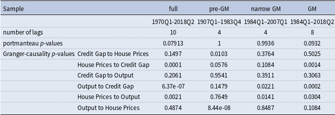
I choose as the baseline model the four-variable model of credit gap, house prices, output, and the FED funds rate. The number of lags is chosen according to Akaike’s information criterion, subject to the Portmanteau test not rejecting its null hypothesis at 95% confidence. Table 1 summarizes key statistics of the baseline VAR models of the analysis. I also run bivariate VARs between credit gap, house prices, and output to confirm the findings in a simplistic setting that helps to understand the effects between variable pairs in isolationFootnote 20 . In addition, I estimate a five-variable VAR model that adds the inflation rate to the variables of the baseline model.
Baseline VAR key statistics

Note: This table summarizes the key statistics of the baseline VAR model estimated on four different subsamples. The table lists the number of lags, the p-values of the Portmanteau tests on serial correlation, and Granger-causality tests of the variable pairs listed in the first column.
3.3. Results
This subsection describes the results from the exercises outlined in the previous subsection. To keep the exposition simple and concise, I show only the results of the baseline VAR model of credit gap, house prices, output, and the interest rate in the main body of the text. The full results of the bivariate analysis and the inclusion of inflation can be found in the online Appendix G.
I first show that volatility has shifted to more medium-cycle fluctuations in the course of the Great Moderation. Then, I show the existence of the Granger-causal relationship between the credit gap and output and discuss the differences between the estimates on the pre-GM and GM sub-periods. The empirical characterization of the Great Moderation and its connection to the financial cycle is then pieced together from the results of the different exercises.
The first important observation stems from the analysis of the spectra prior to and during the Great Moderation. Figure 2 shows the spectra of output, credit gap, and house prices that were estimated on the pre-Great Moderation (1970Q1–1983Q4) and Great Moderation sample (1984Q1–2018Q2). Output volatility has shifted dramatically toward longer periodicities, confirming the finding of Crowley and Hallett (Reference Crowley and Hallett2015). While the spectrum of the pre-Moderation sample features two peaks (near 10 and 28 quarters per cycle), the Great Moderation spectrum has only one peak near 60 quartersFootnote 21 . Volatility decreased on most short-cycle periodicities during the Great Moderation, but it increased on most medium periodicities and all long periodicities. In fact, the Great Moderation spectrum exceeds the pre-Moderation spectrum on all periodicities greater than 24 quarters per cycle. These effects are also found when the narrower definition of the Great Moderation (1984Q1–2007Q1) is applied, as is shown in Figure A.9 in the appendix. The spectra of credit gap and house prices have also moved toward longer periodicities: their peaks have moved from medium-cycle to long-cycle periodicities, and their volatility on short-cycle periodicities disappeared almost entirely. Compared to output, the changes in the spectra of credit gap and house prices are even larger. Volatility of output has increased 4-fold, whereas volatility of credit gap and house prices have increased 6-fold and 20-fold, respectively. The shifts toward longer periodicities are also larger in the financial cycle variables, especially for the credit gap.
Spectra pre-GM and GM: output, credit gap and house prices.
Note: This figure shows the spectra of output (left panel), credit gap (middle panel), and house prices (right panel) estimated on the time series of the pre-GM (light blue) and the GM (dark blue) sample. The left axis measures the variance of the pre-GM spectrum. The right axis measures the variance of the GM spectrum. The x-axis is the periodicity, that is, the number of quarters per cycle of the fluctuations for which the measure is calculated. The spectra are normalized such that for each variable, the higher peak has a maximum of one.

This means that both the business cycle and the financial cycle have increased substantially in length short-term fluctuations of these variables have all given way to longer-term fluctuations. The increases in output volatility on long-cycle periodicities and in credit gap and house price volatility shown here imply that the characterization of the post-1984 US economy as a “moderation” not only falls short, but misses the most important structural changes in the nature of economic and financial fluctuations.
The first piece of evidence that substantiates the importance of the financial cycle to the changes of the Great Moderation comes from the dynamic correlations in combination with the Granger-causality statistics implied by the baseline VAR models. Consequently, they are plotted together in Figure 3, in the left and right columns, respectively. In the dynamic correlation plots, the dashed lines represent 95-%-confidence bounds that are calculated from bootstrapping the coefficients of the VAR model. The top row shows the estimates from the pre-GM sample, the middle row the estimates from the narrow-GM sample, and the bottom row the estimates of the GM sample. By construction, dynamic correlation is between minus one and one.
Dynamic correlation and Granger Causality between credit gap and output.
Note: This Figure shows the dynamic correlations (left column) and the F-statistics of the Granger-causality test (right column). These measures are calculated on data from 1970Q1–1983Q4 (top row), 1984Q1–2007Q1 (middle row), and 1984Q1–2018Q2 (bottom row). The x-axis is the periodicity, that is, the number of quarters per cycle of the fluctuations for which the measure is calculated. Dynamic correlation is measured on a y-axis from −1 to 1. The y-axis of the Granger-causality test measures the F-statistic. The solid lines show the F-statistic at each periodicity, where the legend shows the cause variable of each test. The dashed line is the 95% threshold of the Granger test.

FEVD for the pre-GM (left), narrow GM (middle), and GM (right) sample.
Note: This figure shows the frequency-domain FEVD of output derived from the baseline VAR-model. The left panel was estimated on data from 1970Q1–1983Q4. The panel in the middle was estimated on data from 1984Q1–2007Q1. The right panel was estimated on data from 1984Q1–2018Q2. The x-axis is the periodicity, that is, the number of quarters per cycle of the fluctuations for which the measure is calculated. The y-axis shows the contribution of each shock to the overall forecast error variance.

The dynamic relationship between the credit gap and output is negative on most short-cycle periodicities. It transitions into positive territory on medium-cycle periodicities and is positive on all long-cycle periodicities. While the magnitude of the dynamic correlation coefficients decreases in absolute terms from pre-GM to GM sample, the periodicity ranges on which it is positive and negative remain largely the same in all three samples. Importantly, the periodicity range on which the dynamic correlation coefficient is negative closely matches the range on which the output spectrum shows decreases in volatility. Conversely, the periodicity range on which output gained volatility during the Great Moderation corresponds to the positive dynamic correlation coefficient of credit gap and output.
I pair the dynamic correlations with the results of the Granger-causality tests in the right column. The solid lines show the F-statistics of the tests for Granger-causality at each periodicity. The dashed line is the 95% confidence threshold for these tests. The periodicity at which the test statistic reaches its maximum describes the fluctuations of y, which are predicted most powerfully by x. If the Granger test is not significant on a certain periodicity range, this confirms that the economic forces are only relevant in a periodicity range around the peak of the test-statistic. This range must be interpreted with caution: the test statistics are a continuous function F(ω˜). Hence, even when there is only a causal effect on one specific periodicity, the test will still reject the null hypothesis of Granger-non-causality on the neighboring periodicities.
Prior to the Great Moderation, output Granger-caused the credit gap, and the significance of this relationship was monotonically increasing toward longer periodicities. At this time, the reverse was not true. During the Great Moderation, both variables Granger-cause each other. In the narrow-GM sample, the significance of the Granger-causality of credit increases monotonically toward longer periodicities. On the other hand, the F-statistics when output is the cause variable reach their peak already on short-cycle periodicities and decline thereafter. The GM sample shows that the credit gap and output Granger-cause each other at fundamentally different periodicities. The peak of Granger-causality of output on credit gap is located near 8 quarters and thereby within the short-cycle periodicities. For longer-cycle fluctuations of the credit gap, output exerts less Granger-causal influence, as the test statistic of the Breitung–Candelon tests decreases substantially, yet stays well above the significance threshold. In contrast, the credit gap’s Grangercausality on output is insignificant for a range of short-cycle periodicities. It then increases for longer-cycle fluctuations and attains its maximum on long-cycle periodicities. The finding that the dynamic correlation of credit gap on output is no longer significantly positive for cycles longer than 64 quarters in the longer post-GM sample (third row of Figure 3) is driven by the presence of the Great Recession in the post-GM sample. When the dynamic correlation is estimated only on data between 2010 and 2018, it increases monotonically for medium cycles and long cycles, as shown in Figure A.9.
The combination of dynamic correlation and Granger-causality statistics points to the following relationship between the credit gap and output: A short-cycle downturn in output (Granger-) predicts a short-cycle upswing of the credit gap. In turn, the upswing in the credit gap predicts an attenuation of the downturn in output. However, moving through medium-cycle and long-cycle periodicities, the effects change: A medium-cycle credit boom predicts an output boom, but when the credit gap falls into a medium-cycle trough, one should expect that it draws output with it as well. In other words, credit movements amplify long-cycle movements of output. Figures G.14–G.16 in the online appendix show the results for bivariate models between credit gap, house prices, and output, which confirm my findings.
The second piece of evidence shows the changes in the relationship between the financial cycle and the business cycle that caused the shifts in the spectrum that were pointed out earlier. This is derived from the results of the FEVD of the baseline VAR model, seen in Figure 4, which shows two things: first, before the Great Moderation, neither of the financial cycle variables played a major role. Most of the forecast error in the pre-GM sample is driven by monetary shocks. However, in the Great Moderation sample, the structural shocks to the credit gap and house prices have gained significantly in importance relative to output shocks during the Great Moderation. Both financial shocks have in common that they exert most of their influence on medium-cycle and long-cycle output fluctuations, while short-cycle output fluctuations are largely driven by real shocks (structural innovations to output). Depending on whether the narrow or wide definition of the Great Moderation is applied, the forecast error share is attributed either to credit shocks or house price shocks. The periodicities on which the forecast error share of either financial shock increases the most fluctuations between 16 and 20 quarters—are very close to the periodicity where the dynamic correlation between credit gap and output transitions from negative to positive. Financial shocks systematically lead to lower volatility on short-cycle periodicities but to more volatility on medium-cycle periodicities than output shocks. This phenomenon was observed during the Great Moderation.
3.4. Robustness
I check the robustness of these results along three dimensions. First, I show that the main properties of dynamic correlation and FEVD also hold in the bivariate VAR models as well as when inflation is added to the baseline specification. The qualitative properties of the dynamic correlation and FEVD described above also hold in the VAR model that includes inflation.
Dynamic Correlation is negative on short-cycle periodicities and positive on medium-cycle periodicities. The effects are Granger-causal, and importantly, the Granger-causal effect from output to credit gap is more clearly significant on shorter periodicities. The dynamic correlation between house prices and output is close to zero on short-cycle periodicities but significantly positive on long-cycle periodicities. The significance of Granger-causality from house prices to output rises toward longer periodicities. If anything, the Granger-causality from output to house prices is more strongly significant on short-cycle periodicities.
The forecast error variance decompositions show roughly the same pattern. Orthogonal innovations of output are the dominant driver of only short-cycle periodicities but have little effect on longer periodicities in the samples that include the Great Moderation. In contrast, the innovations to the financial variables lead to forecast error mostly on long periodicities, especially the innovations to the credit gap. The variance attributed to monetary shocks comes in between and attains its maximum forecast error variance share at around 20 quarters per cycle. Inflation behaves similarly to the financial variables, driving very little forecast error at short periodicities and a lot at long-cycle periodicities. These results can be seen in the online appendix G.17.
Secondly, I show that the dynamic correlation pattern is not driven by any particular period in the data. Specifically, I assess the robustness in the following sub-samples: The post-war economy (1946–1983), the Bretton-Woods era (1944–1976), the narrowly defined Great Moderation (1983–2007)Footnote 22 and the longest possible pre-GM sample available in the (annual) JST data (1893–1983). The plots of dynamic correlation, Granger-causality, and forecast error variance decomposition can be seen in Figures A.9 and G.18 in the appendix and online appendix, respectively. The results hold without qualifications when the narrow definition of the Great Moderation is applied. They also hold in the Bretton-Woods and post-war sub-sample with some qualifications: The dynamic correlation between credit gap and output is negative for short-cycle fluctuations (< 4 years) before becoming positive on medium-cycle fluctuations—however, it turns negative again for periodicities beyond 7 yearsFootnote 23 . The effects between house prices and output are Granger-causally driven by output on short periodicities and driven by house prices on long periodicities, each time with a positive coefficient. The FEVD of the Bretton-Woods era tells a different story from the GM one. The financial cycle has next to no relevance as a driver of volatility. Additionally, monetary shocks drive most short-cycle volatility, and output is the main driver of medium-cycle fluctuations. The same results cannot be found in the very long-run pre-GM sample.
Finally, I confirm that the results are not driven by the choice of filter. I obtain similar results when using a one-sided HP filter to remove the trend (see online appendix G.19).
3.5. An accurate picture of the great moderation
The results shown above propose a novel interpretation of the forces at work during the Great Moderation. An accurate characterization of the Great Moderation must primarily point to a transfer of volatility from short-cycle fluctuations to medium-cycle fluctuations, shown by Crowley and Hallett (Reference Crowley and Hallett2015)Footnote 24 (or described as increased persistence by Giannone et al. (Reference Giannone, Lenza and Reichlin2008), Pancrazi (Reference Pancrazi2015)), but also to a shift in the source of those fluctuations from the real to the financial sector. At medium periodicities, the US economy witnessed increases in volatility which are especially pronounced for the credit gap and house prices (where volatility has increased 6-fold and 20-fold, respectively). The structural error decomposition has shown that in this periodicity range, output fluctuations are primarily driven by financial shocks. Hence, one must infer that the origin of output volatility has gravitated to the financial sector.
These shifts are not driven by the Great Recession of 2008 (see Figure G.12 in the online appendix). Hence, even when the narrow definition of the Great Moderation is applied, it was not as moderate as its name suggests. The volatility between 1984 and 2007 was merely a prelude to the dramatic downturn that came with the Great Recession. While there may be multiple reasons for the increases in persistence of output volatility, it fits into the picture of a finance-driven Great Moderation that the financial cycle itself, that is, the dynamic interaction of credit gap and house prices, has shifted to longer periodicities in the course of the Great Moderation. This is shown in Figure G.13 in the online appendix: the range in which this dynamic correlation is strongly positive shifted significantly toward medium-cycle periodicities. This shift across periodicities in the dynamic correlation of the credit gap and house prices is far greater than the shifts in the dynamic correlations between the credit gap and output or house prices and output. Instead, the most significant changes to the latter relationships that came with the Great Moderation concern the development or strengthening of Granger-causality on output, and the diminution of the reverse effect. Rather, the fact that the qualitative properties of the dynamic correlations regarding attenuation and amplification were already present before the Great Moderation suggests the presence of a structural link between credit and output, which is not a product of any mechanism that the literature has used to explain the Great Moderation. The story of the Great Moderation must hence be about the intensification of the previously existing links between the real and financial sectors of the economy and the stronger attenuation and amplification forces that resulted from it. This intensification of the existing volatility transmission mechanisms, coupled with the increased persistence of the financial cycle, then leads to the heterogeneous phenomenon witnessed over the past 35 years: Episodes of moderation with low short-cycle volatility and finance-driven phases in which medium-cycle output volatility surfaces in the form of great recessions.
These findings sideline the academic debate on whether “good luck” or “good policy” drove the Great Moderation. My analysis nevertheless allows me to comment on the positions of this debate. The first main comment is that there was indeed “good luck.” An analysis of the structural innovations (Figure G.21 in the online appendix) shows that a reduction in the error variance did occur in the 1980s and affected both real and financial variables. However, the error variance did not remain low until the Great Recession. Instead, it rose sharply in the 1990s and early 2000s, which points again toward the result that the Great Recession was part of a medium-term fluctuation and not of a sudden increase in short-term volatility. Concerning “good policy,” notice that the contribution of monetary shocks to the forecast error of output has decreased substantially in the course of the Great Moderation. However, mirroring the finding of Crowley and Hallett (Reference Crowley and Hallett2018), it is hard to call the effects of either shocks or policy “good” while I argue that overall volatility has increased on medium-cycle periodicities.
4. Model
This section shows that while off-the-shelf models with financial frictions largely fail to replicate the frequency-domain statistics, a model with long-run risk and the right set of financial frictions can largely replicate the frequency-domain statistics shown in the data.
I build and estimate a model that nests the financial sectors of Iacoviello (Reference Iacoviello2005) (abbreviated “IAC” in the following) and Gertler and Karadi (Reference Gertler and Karadi2011) (abbreviated “GK”) and the combination of the two in a New Keynesian economy. These financial sectors are characterized by a collateral constraint on entrepreneurial borrowing and a leverage constraint on financial intermediaries, respectively. Throughout the rest of this paper, I refer to the model with both collateral and leverage constraints as the “IGK model.”
The key shortcoming of all submodels is that, in contrast to the data, financial shocks never feed systematically into medium-cycle fluctuations. To reconcile the model and data, I show that the inclusion of long-run risk elements in the spirit of Bansal and Yaron (Reference Bansal and Yaron2004) can mitigate this shortcoming. The resulting submodel with both frictions can be calibrated to fit the data well. In contrast to Crowley and Hallett (Reference Crowley and Hallett2018), who reproduce the volatility transfer with a three-equation New-Keynesian model, my model centralizes the financial sector and shows how the interaction of financial frictions and long-run risk can replicate the features of the data. The model also allows me to perform monetary policy counterfactuals that show how a central bank’s reaction to financial market conditions can affect the volatility transfer across frequencies.
The basic framework is a New Keynesian economy, which is enriched with elements found to be of quantitative importance by Smets and Wouters (Reference Smets and Wouters2003). I further set up the model in the spirit of Christiano et al. (Reference Christiano, Eichenbaum and Evans2005) to maintain a close mapping between the model and the identifying restrictions of the structural VARs. For expositional purposes, I focus only on the financial frictions. The model equations are shown in Appendix C, and a more detailed description can be seen in the online appendix.
To finance themselves, entrepreneurs can borrow from a financial intermediary through one-period loans. As in Iacoviello (Reference Iacoviello2005), a framework of costly state-verification introduces a financial friction into the economy, assuming that banks can recover a share
 $\zeta $
of their loans, which leads to the well-known financial accelerator of Kiyotaki and Moore (Reference Kiyotaki and Moore1997). The modeling of the financial intermediaries (banks) follows Gertler and Karadi (Reference Gertler and Karadi2011). In this framework, the managers of financial intermediaries (banks) can divert a fraction
 $\lambda $
of the assets that they manage back to their household, resulting in a moral hazard problem. The incentive constraint that resolves this problem restricts the bank’s ability to lever up—it must accumulate net worth to use alongside deposits to lend to entrepreneurs. As a consequence, the bank may not be able to raise enough deposits to satisfy the entrepreneurs’ demand for credit at a lending rate that equals the deposit rate. Hence, the lending rate in the GK framework will exceed the deposit rate whenever the leverage constraint is binding. When both frictions are active at the same time, they interact as follows: At the steady-state, the values of
 $\zeta $
and
 $\lambda $
determine which constraint is binding. For very low values of
 $\lambda$
, the leverage constraint will be non-binding, and the interest rate will equal the inverse of the households’ discount factor. As
 $\lambda$
increases, the leverage constraint tightens and eventually starts binding. The binding leverage constraint leads to a shortage in credit supply, which leads to an increase in the lending rate. For sufficiently high
 $\lambda$
, the collateral constraint stops binding and only the leverage constraint binds, as the leverage constraint has made credit so expensive that entrepreneurs will no longer borrow up to their collateral constraint.
The financial frictions
 $\zeta$
and
 $\lambda$
are also used to introduce financial supply shocks into the model. That is,
 $\zeta$
and
 $\lambda$
follow AR(1) processes with persistences
 $\rho _{\zeta }, \rho _{\lambda }$
and standard deviations
 $\varepsilon _{\zeta }, \varepsilon _{\lambda }$
. This generates an “active” financial accelerator that is not solely a propagator, but also a source of shocksFootnote
25
. The rest of the model is very close to workhorse models of the literature, most of it borrowed from Villa (Reference Villa2016).
I show that Bayesian-estimated forms of this model are unable to replicate the main frequency-domain statistics of the data in Figures D.10 and D.11. Specifically, I document this failure for the dynamic correlations for the pairs credit gap and output, house prices and output, and credit gap and house prices, for the spectra, and the FEVD of output. Two discrepancies between the model and data arise consistently: firstly, no matter which financial friction is used, the model generates a dynamic correlation between credit gap and house prices that is positive on short periodicities and decreases toward longer periodicities. In other words, the models contain a financial cycle that is a short-cycle phenomenon. This stands in contrast to the data where this interaction, the financial cycle, was shown to be a medium-cycle phenomenon, described by a dynamic correlation that only turned significantly positive on medium-cycle periodicities. Secondly, all submodels generate forecast error shares that are relatively flat across periodicities. Hence, the property of the data that TFP shocks drive short-cycle fluctuations while financial shocks drive medium-cycle fluctuations is not contained in the model.
The dynamic correlations between credit gap and output and between house prices and output also show large departures from their data counterparts, albeit in less consistent ways, as is shown in Figure D.11. The key ingredient that these models are missing is long-run riskFootnote
26
. Long-run risk mechanically leads to a shift of spectral density toward longer periodicities. To ensure that financial shocks drive medium-cycle volatility, I augment the stochastic process of
 $\lambda _{t}$
and
 $ x_{t}$
(an investment cost shock that capital producers are subject to) by long-run risk components in the spirit of Bansal and Yaron (Reference Bansal and Yaron2004):
 \begin{align} x_{t}&=e_{t}^{x}+s_{t}^{LR_{x}}\end{align}
 \begin{align} s_{t}^{LR_{x}}&=\rho _{x}s_{t-1}+e_{t}^{LR_{x}}\end{align}
 \begin{align} \lambda _{t} & = e_{t}^{\lambda }+s_{t}^{LR_{\lambda }}\end{align}
 \begin{align} s_{t}^{LR_{\lambda }} & = \rho _{\lambda }s_{t-1}+e_{t}^{LR_{\lambda }}\end{align}
Hence, the composite process features both short-run and long-run risk. To maintain a close mapping between empirical and model-based analysis, I impose timing assumptions on the model in the spirit of Christiano et al. (Reference Christiano, Eichenbaum and Evans2005). The timing of the model, which gives rise to the identifying restrictions, is discussed in detail in the online appendix. The model is calibrated in close accordance with the literature (see Villa (Reference Villa2016), Gertler and Karadi (Reference Gertler and Karadi2011), and Iacoviello (Reference Iacoviello2005)), and the values are reported in Table I.3 in the online appendix. Under the benchmark parameterization from Table I.3, only the collateral constraint is binding (Iacoviello model). However, when the fraction of divertable funds is increasedFootnote
27
, both leverage and collateral constraint bind in steady-state. The collateral constraint can be deactivated by setting
 $\zeta = \infty .$
The remaining parameters are calibrated to fit the model to the data. Herein, I use simulated method of moments to target the empirical dynamic correlations for the variable pairs credit gap and output, credit gap and house prices, and house prices and output. Additionally, I target the FEVD estimated by the four-variable VAR of credit gap, house prices, output, and the policy rate. Therefore, I pick the policy parameters of the Taylor rule, persistences, and standard deviations of the shocks to minimize the distance between the model and data moments. Given that the empirical targets consist of one moment for each frequency, the model is over-identified. For further details on parameterization and calibration, I refer the reader to the online Appendix J.1. I calibrate each sub-model separately for the pre-GM and GM period. For expositional reasons, I only discuss the calibration of the best-performing submodel here: the framework that combines collateral and leverage constraint. The calibrated parameters of this submodel are shown in Table J.4. There are three important changes between the two periods: Firstly, central bank policy responds more to inflation and the output gap in the Great Moderation period than prior to the Great Moderation, but the importance of interest rate smoothing has decreased. Secondly, the persistence of TFP shocks has increased from 0.364 to 0.9701, while the persistence of mark-up shocks has decreased from 0.4478 to 0.1153. Thirdly, there are also important changes in the standard deviations of the shocks. The standard deviation of the short-run investment cost shock has increased 5-fold, and the standard deviation of the long-run risk shock has increased even sevenfold. Meanwhile, the standard deviations of the financial shock, TFP shock, monetary shock, and mark-up shock have fallen.
Figure 5 shows the spectra of the model-generated data. As can be seen, both GK and IAC models perform poorly. The models generate too much long-cycle volatility for both samples. While the IAC model at least produces more short-cycle volatility in the calibration to pre-GM data, the spectra implied by the GK model do not have any of the qualitative properties of the empirical spectra. The IGK model replicates the feature that short-cycle volatility has decreased relative to medium-cycle volatility in the GM sample. However, it does not replicate the overall shift toward longer periodicities. The peak of the spectrum of the IGK model calibrated to fit the pre-GM moments is already on financial cycle periodicities. Figure 6 shows how the model-implied dynamic correlations between credit gap and output and the FEVD of output compare to their data counterparts.
Spectra of model-generated data.
Note: This figure shows the spectra of the calibrated models. The x-axes are the periodicities, that is, the number of quarters per cycle of the fluctuations for which the measures are calculated. The y-axes show the variance and the respective periodicity.

Dynamic correlation and FEVD: model versus data.
Note: This figure shows how the model-implied dynamic correlations and FEVD compare to their data counterparts of the baseline VARmodel. The top two rows show the results when the model is calibrated to fit the moments from the estimates on data between 1970Q1–1983Q4. The bottom two rows show the results when the model is calibrated to fit the moments from the estimates on data between 1984Q1–2018Q2. The x-axes are the periodicities, that is, the number of quarters per cycle of the fluctuations for which the measures are calculated. The y-axes measure the dynamic correlation on a scale from −1 to 1. The y-axes of the FEVD plots measure the contribution of the orthogonal shock to the variable listed in the legend to the overall forecast error variance.

First and foremost, the model with both collateral constraint and leverage constraint (IGK model) is the best fit to the data. It outperforms the models with only one financial friction, especially regarding the FEVD and the spectrum. The model with only a collateral constraint (IAC) matches the dynamic correlations between credit gap and output well, but misses on spectrum and FEVD, while the model with only a leverage constraint misses on all three statistics.
In both pre-GM and GM samples, the IGK model replicates the qualitative properties of the frequency-domain statistics of the data. The dynamic correlation between credit gap and output is negative on short periodicities and positive on medium periodicities. In the pre-GM sample, the model-implied dynamic correlation is flatter than the empirical estimate and only turns positive on long periodicities rather than on medium periodicities. In the GM sample, the model-implied dynamic correlation closely tracks the empirical one but somewhat overshoots the dynamic correlation of the data on long periodicities. Interestingly, the IAC model follows the data more closely in this area, so that I can conclude that the low dynamic correlation of long cycles in the GM sample is driven by a financial accelerator effect. This fits the fact that the low dynamic correlation on long cycles is driven by the presence of the Great Financial Crisis in the GM sample, which was characterized by a large (downward) financial accelerator.
The model-implied FEVD of the IGK model also replicates most qualitative and even quantitative properties of the empirical FEVD: In the pre-GM sample, it replicates the large forecast error share of monetary shocks that still increases on longer periodicities. It largely replicates the forecast error share of TFP shocks that decreases in importance on longer periodicities. It also acknowledges the minor role that financial shocks played before the Great Moderation. In the GM sample, the model exhibits the feature that short-cycle fluctuations are mainly driven by TFP shocks, whereas medium-cycle and long-cycle fluctuations are driven by financial, especially asset price shocks (investment cost shocks in the model). It matches the forecast error share and the periodicities that investment cost shocks feed into closely. The most obvious shortcoming of the model is that it somewhat underestimates the role that monetary shocks played in the GM, especially on medium-cycle and long-cycle periodicities. In contrast, the FEVDs of IAC and GK model do not have the targeted feature that financial shocks mainly feed into medium-cycle periodicitiesFootnote 28 .
Despite all successes, the IGK submodel still falls short on the other targeted moments. The dynamic correlations that it produces between house prices and credit gap, and house prices and output, are positive on short periodicities and decrease (sometimes become negative) on longer periodicities (Figure J.23). As discussed previously, in the data, the opposite is the case—these dynamic correlations should increase toward longer periodicities. This disparity between model and data is shared by all submodels. The difficulty of any model from the literature in producing a dynamic correlation between credit gap and house prices that increases toward longer periodicities indicates that this problem may be systematic. The construction of a model that contains a medium-term financial cycle is thus a task that still requires more attention in future research.
5. Discussion
The estimated parameters shed light on the changes that define the Great Moderation. First, the largest changes are the increases in the standard deviations of the investment cost shocks. These changes directly affect house prices in the model, which are responsible for the largest part of medium-cycle volatility. The long-run risk shock has gained in variance even more than the short-run component. The financial supply shock has seen reductions in the standard deviations of both its short-run and its long-run components, and the short-run component has decreased relative to the long-run component. Hence, the calibrated parameters suggest that a key feature of the Great Moderation was an increase in long-run risk relative to short-run risk, a similar finding as in Pancrazi (Reference Pancrazi2014). Hence, I argue that the “good luck hypothesis” can be refined with respect to the medium-run: There was indeed “good luck” but only concerning the short-run risk, but through the financial sector, there was no good luck in the medium run. A short-run reduction of risk was also detected in the standard deviation of the TFP shock size in the GM sample, which points toward “good luck” as a relevant contributing factor to the Great Moderation. The small changes to the persistence and the standard deviation of the mark-up shocks indicate that the model assigns at most a minor role to inflation as a driver of the Great Moderation.
Secondly, the fact that only the combined Iacoviello + Gertler-Karadi financial sectors in combination are able to replicate the frequency-domain properties of the data emphasizes the importance of modeling both collateral and leverage constraints and offers further insights into the mechanics by which shocks feed into fluctuations of different periodicities. In the pure Iacoviello framework, the interest rate is purely determined by the difference between the discount factors of the patient household and the lender. Hence, if a shock hits the collateral constraint, it transmits immediately to the entrepreneurial capital holdings and thereby affects production. In combination with the Gertler-Karadi friction, the lending rate increases in response to a negative shock on the banks’ maximum leverage and thereby can absorb the immediate effect of the shock. Paired with the long-run risk persistence of the shock to the credit supply technology of the banks, this can then feed into much longer fluctuations than shocks that hit the collateral constraint directly.
Despite the success of the long-run risk-augmented model in replicating those key features of the data, long-run risk remains a mechanical way of increasing the persistence of volatility in the model. This relates to the well-known issue that RBC models only generate persistence when it is explicitly built into the model. A model that contains an accurate financial cycle in the form of a purely medium-cycle interaction between credit gap and house prices that can endogenously generate the frequency-domain statistics would enhance the understanding of the relationship between the real and financial sectors more than the notion of long-run risk.
I can use the model to run “counterfactuals” to isolate the effects that result from the changes in the Taylor Rule, the persistences of the shocks, and the shock sizes. I calculate these by re-running the model calibrated to pre-GM (GM) data while replacing the relevant values with those estimated from GM (pre-GM) data. The results are shown in Figures J.27 and J.28 and yield interesting insights: In the pre-GM model economy with the GM Taylor Rule, there is lower short-cycle output volatility, but more medium-cycle output volatility compared, as can be seen in Figure 7.
Monetary policy counterfactuals: inflation and output gap aversion.
Note: This Figure shows summary statistics of the monetary policy counterfactual. This is calculated by using the pre-GM estimates of the model and substituting the Taylor Rule coefficients with the GM-estimated values. The left subfigure shows the resulting spectra of the pre-GM model, GM model, and counterfactual. Equivalently, the middle subfigure shows the corresponding dynamic correlations. The right subfigure shows the FEVD of the counterfactual.

Additionally, the investment shock already drives systematically medium-cycle fluctuations. In contrast, the contribution of financial shocks to the output forecast error is small and relatively flat in a hypothetical GM economy with the calibrated pre-GM Taylor Rule. This suggests that monetary policy may have contributed to the effects of financial markets on medium-cycle volatilityFootnote 29 . Hence, I argue that the “good policy” hypothesis of the Great Moderation can also be refined with respect to the medium-run implications of monetary policy.
At the same time, the change in the Taylor Rule does not affect the dynamic correlations between the credit gap, house prices, and output much. The analog experiments can be run to test the effects of changes to the shocks’ persistences and standard deviations. When I reset the persistences to the values of the other period, I also adjust the shock sizes to ensure that the overall variance of the stochastic process remains constant. The details of this exercise are in Appendix J.3 Footnote 30 . Their results imply that changes to the persistences greatly amplified the contribution of the financial shocks to the forecast error of output. On top of that, they show that the qualitative property of financial shocks feeding systematically into medium-cycle volatility vanishes easily when any of the coefficients are replaced by their counterparts from the other sub-period. This re-emphasizes the fact that only a combination of multiple model ingredients can replicate the features of the Great Moderation and its relationship with the financial cycle. Finally, Figure 8 shows the result of a monetary policy that reacts to build-ups of the credit gap, that is, leans against the wind. Here, a small aversion against a large credit gap is built into the calibrated Taylor rule of the post-GM era. As can be seen in the left panel of Figure 8, this change shifts the peak of the spectrum slightly to the left. It induces more volatility of cycles shorter than roughly 16 years, but less volatility on very long cycles longer than 16 years. This shows that in addition to the lower inflation aversion or higher output stabilization aversion outlined in Crowley and Hallett (Reference Crowley and Hallett2018), leaning against the wind is another way to reduce the shift of volatility to long cycles.
Monetary policy counterfactual: leaning against the wind.
Note: This Figure shows the spectrum, dynamic correlation, and FEVD of the monetary policy counterfactual when the central bank is reacting to excessive credit gaps. The other parameters of the Taylor Rule are those of the post-GM calibration.

6. Conclusion
In this paper, I have shown that the defining features of the Great Moderation were a shift of volatility to longer periodicities and a shift in the source of volatility to the financial sector, confirming the results of Crowley and Hallett (Reference Crowley and Hallett2015) and extending them by documenting the role of the financial cycle. The latter shows up in the data as a systematic manifestation of financial shocks into medium- and long-cycle output fluctuations. On top of that, I showed that a frequency-domain analysis reveals previously undiscovered properties of the interaction of the business cycle with financial cycle variables. I documented a Granger-causal mechanism between the credit gap and output that features attenuation forces on short periodicities but amplification forces on medium- and long-cycle periodicities. This mechanism is not linked to a specific period. Hence, I argued that it should be thought of as structural. I use this evidence to argue that the Great Moderation and the Great Recession are inextricably tied together. The former was a consequence of the short-cycle attenuation forces, whereas the latter was an inevitable result of the amplification forces.
These features are only improperly replicated by off-the-shelf quantitative DSGE models. The elements Smets and Wouters (Reference Smets and Wouters2003) found to be important to throw sand in the wheels of the model and generate the persistent fluctuations observed in the data, and the financial frictions of Iacoviello (Reference Iacoviello2005) and Gertler and Karadi (Reference Gertler and Karadi2011) do not distinguish accurately between the different period fluctuations that shocks emerging in different sectors of the economy feed into. This led to a disparity between the dynamic correlations of key variable pairs between the model and data. I showed that a long-run risk structure enhances the model’s flexibility in this respect. The interaction of long-run investment cost risk with collateral and leverage constraint gets very close to replicating a) the dynamic correlation between credit gap and output that is negative on short periodicities and positive on long periodicities, and b) shocks on the relative price of capital goods that feed mainly into medium-cycle volatility while leaving short-term volatility relatively unaffected.
I used the estimated parameters of the model to show that the “good luck” hypothesis of the Great Moderation is only true with respect to short-run risk. Meanwhile, long-run risk has increased. I also used a monetary policy counterfactual of the model to argue that the “good policy” hypothesis of the Great Moderation can be refined with respect to the longer-run effects. While the changes in monetary policy during the Great Moderation led to lower short-term output fluctuations, this came at the expense of higher medium-term volatility. An aversion of monetary policy to credit conditions can reduce this shift.
More research is needed to fully understand the mechanisms that led to the Great Moderation and the Great Recession. On the empirical side, this concerns the initial developments that triggered the intensification of the relationship between the real and financial sectors. Additionally, a causal identification of the resulting effects of financial intermediaries and the growth of the financial sector on short- and mediumterm output volatility would greatly enhance the understanding of the linkages that ultimately led to the Great Financial Crisis and the Great Recession. On the theoretical front, the main shortcoming is that the model does not represent the financial cycle, the interaction between credit gap and house prices, accurately. Additionally, at this point, it is not clear whether other existing models are able to replicate the frequency-domain properties outlined above. Fruitful avenues for future research open up: A model that can capture both attenuation and amplification of finance to the real economy, containing a financial cycle that captures the medium-term self-enforcing interactions of credit and house prices and accurately replicate the periodicity structure of output volatility would go a long way toward a deeper understanding of the relationship between finance and the real economy. An accurate understanding of whether an economic situation is truly a fundamental moderation or merely a low-volatility phase of a longer and larger cycle could help predict and prevent great finance-related recessions of the future.
Supplementary material
The supplementary material for this article can be found at https://doi.org/10.1017/S136510052510045X.
Appendix A. Empirical extras
Appendix A.1. Robustness checks with VAR models
Robustness Checks Dynamic Correlation and FEVD.
Note: This Figure shows the dynamic correlations (1st and 3rd row), the F-statistics of the Granger-causality test (2nd and 4th row) and FEVD (bottom row) of the VAR-models with Credit Gap, House Prices, Output, and Interest Rate. In the third and fourth column, the Fed Funds Rate is replaced by the shadow rate of Wu and Zhang (Reference Wu and Zhang2019). In the fourth column, I use the shadow rates, as it is not possible to estimate a stationary VAR on the detrended data when using the Fed Funds Rate.

Appendix B. Frequency-domain tools
Frequency-domain methods build on the Fourier transform, which disaggregates time series into cycles of different frequencies ω ∈ (0,π). The most commonly used frequency-domain tool in economics is the spectrum, denoted S
xx
, which measures how much variance is attributed to the cycles of each frequency. It is calculated as the Fourier transform of the autocovariance function
 $\unicode{x1D6E4} _{xx} = Cov(x_{t},x_{t-j}), j \in (\underline{t},\overline{t})$
of time series
 $x_{t}$
(with
 $\underline{t}\leq t\leq \overline{t})$
:
 \begin{equation}S_{xx}=\frac{1}{2\pi }\sum _{j=\underline{t}}^{\overline{t}}\unicode{x1D6E4}_{xx}^{\left(j\right)}e^{-i\omega j}\end{equation}
In multivariate time series, the (complex) cross-spectrum between two variables x and y is denoted
 $S_{xy}(\omega )$
and describes the co-variance on each frequency—calculated as the Fourier transform of the cross-covariance function
 $\Gamma _{xy}$
.
Assume that the evolution of the variables can be described by a vector-autoregressive process of K variable of p lags each. Without loss of generality, define
 $X=(x,y,z_{1},\ldots ,z_{K-2})$
the variables of the VAR. Each regression equation of the underlying VAR is of the form
 \begin{equation}x_{t}=c_{k}+\sum _{i=1}^{p}a_{i}x_{t-i}+\sum _{j=1}^{p}\beta _{j}y_{t-j}+\sum _{k=1}^{K-2}\sum _{l=1}^{p}\gamma _{k,l}z_{k,t-l}+e_{t}\end{equation}
where
 $c_{k}$
is the equation-k intercept and
 $\alpha _{i}, \beta _{i}$
and
 $\gamma _{k,l}$
are the regression estimates. Transforming the VAR(p) into its VAR(1) form, denote M the companion matrix of the VAR, then
 \begin{equation}\tilde{X}_{t}=M\tilde{X}_{t-1}+\epsilon _{t}\end{equation}
From this state-space form of the VAR, the dynamic correlation
 $P_{xy}$
is calculated asFootnote
31
:
 \begin{equation}P_{xy}\left({\unicode{x03C9}} \right)=\left(I-Me^{-i{\unicode{x03C9}} }\right)^{-1}{\unicode[Arial]{x03A3}} \left(I-Me^{i{\unicode{x03C9}} }\right)^{-1}\end{equation}
where I is a K × K identity matrix and Σ is the estimated covariance matrix of the VAR. The test for frequency-domain Granger-causality tests the hypothesis
 $H_{0}\colon M_{y\rightarrow x}({\unicode{x03C9}} )=0$
that cause variable y does not Granger-cause effect variable x at frequency ω in a bivariate VAR modelFootnote 32 . The corresponding test statistic from Geweke (Reference Geweke1982) is
 \begin{equation}M_{y\rightarrow x}\left({\unicode{x03C9}} \right)=log\left[\frac{2{\unicode[Arial]{x03C0}} S_{xx}\left({\unicode{x03C9}} \right)}{\left| \Psi _{11}\left(e^{-i{\unicode{x03C9}} }\right)\right| ^{2}}\right]\end{equation}
where
 $\Psi (L){\unicode{x03B7}} _{t}=\Phi (L){\epsilon} _{t},\Phi (L)$
is the lag polynomial and
 ${\unicode{x03B7}} _{t}=G{\epsilon} _{t}$
where G is a lower-triangular matrix such that
 $E({\unicode{x03B7}} _{t}{\unicode{x03B7}} _{t})=I$
is an identity matrix. As shown by Breitung and Candelon (Reference Breitung and Candelon2006), this is equivalent to testing a pair of linear hypotheses
 $H_{0}\colon R({\unicode{x03C9}} ){\unicode{x03B2}} =0$
where
 $\beta$
is the vector of estimates and
 \begin{equation}R(\omega )=\left[\begin{array}{ccc} cos(\omega ) & \begin{array}{cc} cos(2\omega ) & \ldots \end{array} & cos(p\omega )\\ sin(\omega ) & \begin{array}{cc} sin(2\omega ) & \ldots \end{array} & sin(p\omega ) \end{array}\right]\end{equation}
Appendix C. Model
Appendix C.1 Households’ problems
There is a mass 1 of identical patient households indexed by i. Households maximize their utility through choice of consumption
 $C_{t}$
, housing
 $K_{t+1}$
, deposits
 $D_{t}$
in a financial intermediary and labor supply
 $L_{t}$
. Their utility from consumption depends on external habit and capital depreciates at rate
 $\delta$
. Housing costs
 $Q_{t}$
and deposits earn interest
 $R_{t-1}$
. Each household owns a bank and receives the its bank’s profits.
Household are subjected to government taxation
 $T_{t}$
and transfers
 $TR_{t}$
. Their maximization problem is:
 \begin{align} & maxE_{t}\sum _{t=0}^{\mathrm{\infty }}\beta ^{t}\left.\left\{log\left(C_{it}-hC_{t-1}\right)-\frac{L_{it}^{1+\Phi _{l}}}{1+\Phi _{l}} + {\unicode[Arial]{x03BD}} log\left(K_{it+1}\right)\right.-\mu _{it}\left[C_{it}+Q\_ t(K_{it+1}-\left(1-\delta \right)K_{it})\right.\right.\nonumber\\& \qquad\qquad\qquad + \left.\left. D_{it+1}-R_{t-1}D_{it}-W_{t}^{H}L_{it}-\sqcap _{t}+T_{t}-TR_{t}\right]\vphantom{\frac{L_{it}^{1+\Phi _{l}}}{1+\Phi _{l}}}\right\}\end{align}
Appendix C.2. Labor unions’ problems
Households supply homogenous labor to monopolistic labor unions which differentiate it and sell an aggregate
 $L_{t}$
. Unions adjust wages according to a Calvo scheme with parameter
 $ \sigma _{w}$
. In a given period, the wages of firms that cannot re-optimize are indexed to inflation. The union maximizes
 \begin{equation}max\, E_{t}\sum _{s=0}^{\mathrm{\infty }}\frac{\mu _{t+s}}{\mu _{t}}\left(\beta \sigma _{w}\right)^{s}L_{t+s}\left(l\right)\left[\frac{W_{t}^{r}\left(l\right)}{P_{t+s}}\left(\frac{P_{t+s-1}}{P_{t-1}}\right)^{{{\unicode[Arial]{x03C3}} _{wi}}}-\frac{W_{t+s}^{H}}{P_{t+s}}\right]\end{equation}
Appendix C.3. Retailers’ problems
Monopolistic retailers purchase intermediate goods at marginal cost from entrepreneurs, differentiate the goods and sell a final good made from the different varieties. Retailers adjust according to a Calvo scheme with parameter σ p . In a given period, the prices of firms that cannot re-optimize are indexed to inflation. The retailers maximize
 \begin{equation}maxE_{t}\sum _{s=0}^{\mathrm{\infty }}\frac{\mu _{t+s}}{\mu _{t}}\left(\beta \sigma _{p}\right)^{s}Y_{t+s}(f)\left[\frac{P_{t}^{r}(f)}{P_{t+s}}\left(\frac{P_{t+s-1}}{P_{t-1}}\right)^{{{\unicode[Arial]{x03C3}} _{pi}}}-\frac{\Phi _{t+s}}{P_{t+s}}\right]\end{equation}
Final output is a composite of the differentiated intermediate goods f ∈ (0,1):
 \begin{equation}Y_{t}=\left[\int _{0}^{1}Y_{t}(f)^{\frac{{\epsilon} -1}{{\epsilon} }}df\right]^{\frac{{\epsilon} }{{\epsilon} -1}}\end{equation}
Final goods firms are competitive and their optimization problems are:
 \begin{equation}min\int _{0}^{1}P_{t}(f)Y_{t}(f)df \\s.t.\overset{-}{Y}\leq \left[\int _{0}^{1}Y_{t}(f)^{\frac{{\epsilon} -1}{{\epsilon} }}df\right]^{\frac{{\epsilon} }{{\epsilon} -1}}\end{equation}
Appendix C.4. Capital producers
Capital producers purchase some of the final goods (as investments
 $I_{t}$
) and transform them into (durable) capital goods. They sell them to the household which consume capital (interpreted as housing) and to entrepreneurs which use the capital to produce. They are subject to a capital quality shock
 $x_{t}$
. The problem of capital producers is:
 \begin{equation}maxE_{t}\sum _{t=0}^{\mathrm{\infty }}\beta ^{t}\sqcap _{t}+{\unicode{x03BC}} _{t}^{K}\left[\sqcap _{t}-\left(Q_{t}^{n}-P_{t}\right)I_{t}+x_{t}I_{t}\left(1-F\left(\frac{I_{t}}{I_{t-1}}\right)\right)\right]\end{equation}
Appendix C.5. Financial intermediaries’ problems
Competitive financial intermediaries (banks) maximize the discounted sum of their future profits. Banks survive a period with probability
 $\theta$
. In case they die, they give their entire net worth back to their household, after which they are immediately reborn and given transfer
 $N^{n}$
by their household.
Banks take deposits from patient households which are paid deposit rate
 $R_{t}$
in exchange. Each bank uses those funds along with its own net worth to provide credit to entrepreneurs. Credit
 $B_{t}^{F}$
comes in the form of simple 1-period bonds and the lending rate is denoted
 $R_{t}^{L}$
Costly repossession: It is assumed that if the debtor fails to repay the loan, the bank needs to pay a cost of
 $\zeta$
to find and repossess one unit of the borrower’s assets. I assume that this cost
 $\zeta$
is stochastic and evolves according to
 \begin{equation}{\unicode[Arial]{x03B6}} _{t}={\unicode[Arial]{x03B6}} _{t-1}^{{\unicode{x03C1}} _{{\unicode[Arial]{x03B6}} }}\overline{\zeta }^{1-{\rho _{\zeta }}}e^{{\epsilon} _{t}^{{\unicode[Arial]{x03B6}} }}\end{equation}
so that its average over time is
 $\zeta$
¯. The bank will ensure itself of repayment by forcing the entrepreneur to pose collateral for the debt:
 \begin{equation}\left(1-{\unicode[Arial]{x03B6}} _{t}\right)Q_{t+1}K_{jt+1}^{F}\left(1-{\unicode[Arial]{x03B4}} \right)\geq B_{jt+1}^{F}\end{equation}
When the entrepreneur does not repay, the bank can pay the repossession cost and will (in expectation) be able to cover its losses completely by selling the entrepreneur’s leftover capital. Hence, the lending rate will equal the deposit rate in the Iacoviello economy.
Moral hazard: Following Gertler and Karadi (Reference Gertler and Karadi2011), the manager of the bank has the option to divert a fraction λ of the bank’s resources back to his household. As the cost of state verification, I assume that λ is stochastic. This gives rise to an incentive constraint in the form of a leverage constraint. This limits the ability of the bank to obtain deposits. This setup leads to the objective:
 \begin{equation}\Upsilon _{t}=maxE_{t}\sum _{i=0}^{\mathrm{\infty }}\left(1-\theta \right)\theta ^{i}{\unicode{x03B2}} ^{i+1}{\unicode{x039B}} _{t,t+i+1}\left(R_{t+i}^{L}B_{t+1+i}^{F}-R_{t+i}D_{t+1+i}-R_{t+i}N_{t+i}\right)\end{equation}
In this optimization,
 ${\unicode{x039B}} _{t,t+1}=\frac{{\unicode{x03BC}} _{t+1}}{{\unicode{x03BC}} _{t}}$
. This yields the constraint
 \begin{equation}V_{t}B_{t+1}^{F}+H_{t}N_{t}\geq {\unicode[Arial]{x03BB}} _{t}B_{t+1}^{F},\end{equation}
which places an upper bound on the leverage of the bank.
Appendix C.6. Entrepreneurs’ problems
There is a mass 1 of entrepreneurs indexed j in the economy. As in Iacoviello (Reference Iacoviello2005) they only consume non-durable goods and use the capital goods to produce new intermediate goods. Entrepreneurs’ production technology is:
 \begin{equation}Y_{t+1}=A_{t}\left(U_{t}K_{t+1}^{F}\right)^{{\unicode[Arial]{x03B1}} }L_{t}^{1-{\unicode[Arial]{x03B1}} }-\Theta\end{equation}
Entrepreneurs also die in each period with probability
 $\theta$
. In this case entrepreneurs are immediately reborn. This effectively shrinks their discount factor and ensures that they will always be borrowing constraint. Accordingly, the problem of the entrepreneur is:
 \begin{align} & maxE_{t}\sum _{t=0}^{\mathrm{\infty }}\left(\gamma \beta \right)^{t}\left.\left\{\frac{\left(C_{jt}^{F}-h^{F}C_{t-1}^{F}\right)^{1-{\Phi _{f}}}}{1-\Phi _{f}}\right.+\mu _{jt}^{F}\left[\Phi _{t}Y_{jt}+B_{jt+1}^{F}-C_{jt}^{F}-W_{t}L_{t}-\Psi \left(U_{jt}\right)K_{jt}^{F}\right.\right.\nonumber\\& \qquad \left.\left.-Q_{t}\left(K_{jt+1}^{F}-\left(1-\delta \right)K_{jt}^{F}\right)-R_{t-1}^{L}B_{jt}^{F}\right]+\mu _{t}^{C}E_{t}\left[\left(1-\zeta _{t}\right)Q_{t+1}K_{jt+1}^{F}\left(1-\delta \right)-R_{t}^{L}B_{jt+1}^{F}\right]\vphantom{\frac{\left(C_{jt}^{F}-h^{F}C_{t-1}^{F}\right)^{1-{\Phi _{f}}}}{1-\Phi _{f}}}\right\}\nonumber\\[5pt]\end{align}
Appendix C.7. Central bank
The central bank sets its policy rate according to the Taylor rule
 \begin{equation}ln\left(\frac{R_{t}^{n}}{R_{t}}\right)={\unicode{x03C1}} _{i}ln\left(\frac{R_{t-1}^{n}}{R^{n}}\right)+\left(1-{\unicode{x03C1}} _{i}\right)\left[{\unicode{x03C1}} _{{\unicode[Arial]{x03C0}} }ln\left(\frac{\sqcap _{t}}{\sqcap _{t-1}}\right)+{\unicode{x03C1}} _{y}ln\left(\frac{Y_{t}}{Y_{t}^{p}}\right)\right]+{\unicode{x03C1}} _{{{\unicode[Arial]{x0394}} _{y}}}ln\left(\frac{Y_{t}/Y_{t-1}}{Y_{t}^{p}/Y_{t-1}^{p}}\right)+{\epsilon} _{t}^{r}\end{equation}
And
 \begin{equation}R_{t+1}=E_{t}\left[\frac{R_{t}^{n}}{\sqcap _{t+1}}\right].\end{equation}
Appendix C.8. Market clearing conditions
Market clearing on final goods market and capital market is given by:
 \begin{align}Y_{t}& =C_{t}+C_{t}^{F}+I_{t}+\Psi \left(U_{t}\right)K_{t}^{F}+G_{t}\\[-10pt]\nonumber\end{align}
 \begin{align} I_{t} & =K_{t+1}-\left(1-{\unicode[Arial]{x03B4}} \right)K_{t}+K_{t+1}^{F}-\left(1-{\unicode[Arial]{x03B4}} \right)K_{t}^{F}\\[-10pt]\nonumber\end{align}
In words, the final goods that are produced in this economy are split between private, entrepreneurial and government consumption of non-durables, investment into durables and maintaining the current capital stock at the chosen utilization rate. On the market for durable capital, total investment is given by the changes in the durables stocks of patient household and entrepreneurs.
Appendix D. Estimation results
The analysis of the model-generated data shows that no financial sector that the model nests replicates the quantitative and qualitative properties of the frequency-domain statistics even to a moderate extent. While the model-generated spectrum of the GM sample shifts toward longer periodicities compared to the pre-GM spectrum, the periodicities at which this occurs are not the same as those observed in the data. All financial sectors also fail to replicate the dynamic correlation patterns of the data. In the model with a collateral constraint (Iacoviello framework) the dynamic correlation between credit gap and output is positive on all periodicities. When a leverage constraint is included (GK and IGK framework) the dynamic correlation is negative on a intermediate range of periodicities, but it is not the same as in the data.
Spectra of model-generated data.
Note: This figure shows the spectra implied by the models, estimated on data from 1970Q1–1983Q4 and 1984Q1–2018Q2. The x-axes are the periodicities, that is, the number of quarters per cycle of the fluctuations for which the measures calculated. The y-axes measure the variance at each periodicity.

Dynamic Correlation and FEVD: Estimated Model.
Note: This figure shows how the moments of the estimated models compare to their data counterparts. The models were estimated on data from 1970Q1–2018Q2. The x-axes are the periodicities, that is, the number of quarters per cycle of the fluctuations for which the measures calculated. The y-axes measure the dynamic correlation on a scale from −1 to 1. The y-axes of the FEVD plots measure the contribution of the orthogonal shock to variable listed in the legend to the overall forecast error variance.

The dynamic correlation between credit gap and output is negative well into financial cycle periodicities. The dynamic correlation between house prices and output, and credit gap and house prices are also replicated inaccurately: In the data they are near to zero and highly positive on financial cycle periodicities, all models generate dynamic correlations that are decrease toward longer periodicities. This is especially clear for the relationship between credit gap and house price, that is, the financial cycle. Their dynamic interaction is medium-term in the data but is consistently produced as short-term in the model. In fact, I run robustness checks with 6 other off-the-shelf models with financial sectors from the literature which all err in the same way with regard to the financial cycle.
Appendix E. Online appendix
The online appendix provides further robustness checks on the empirical part to the paper and shows details on the calculation of the steady state, calibration, estimation, sensitivity analysis and counterfactual analysis of the paper. It can be accessed here: https://sites.google.com/view/friedrichlucke/home.