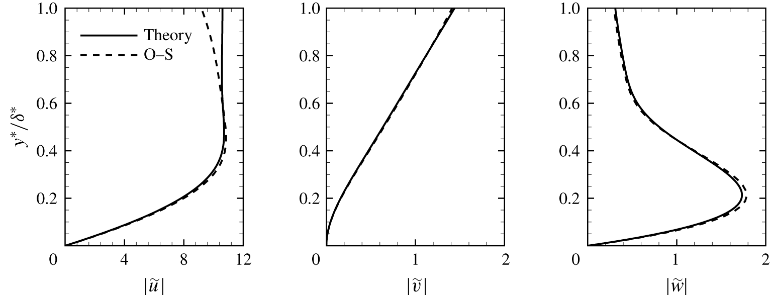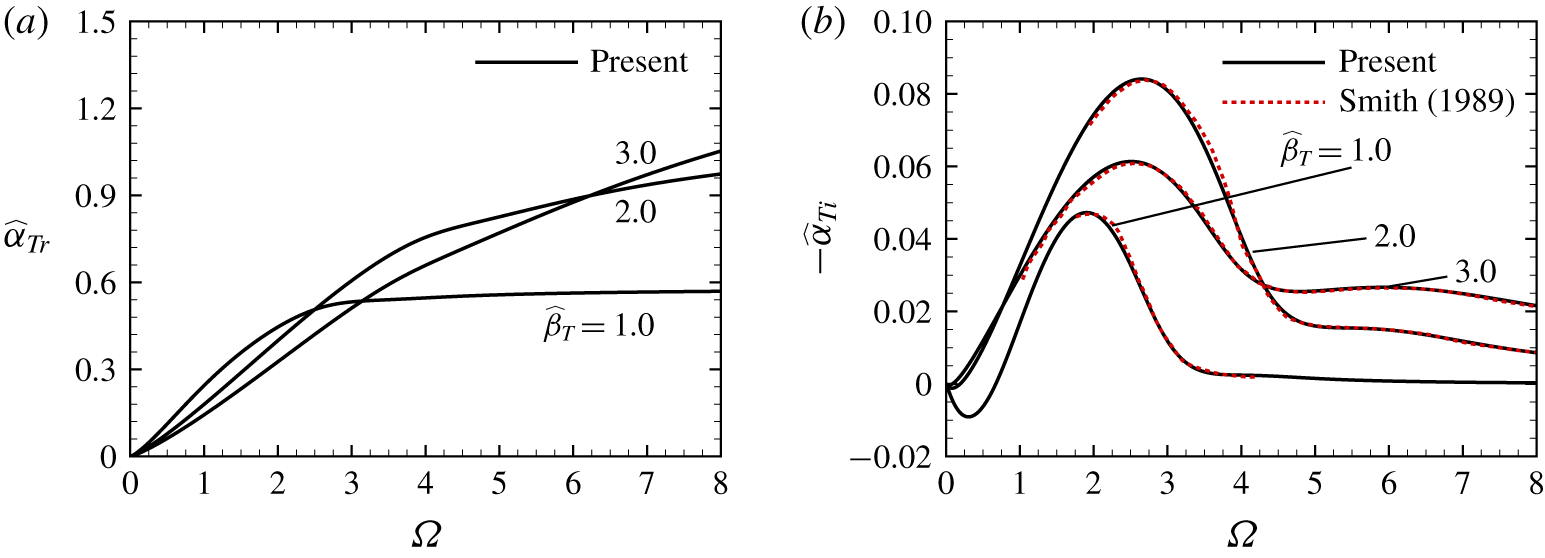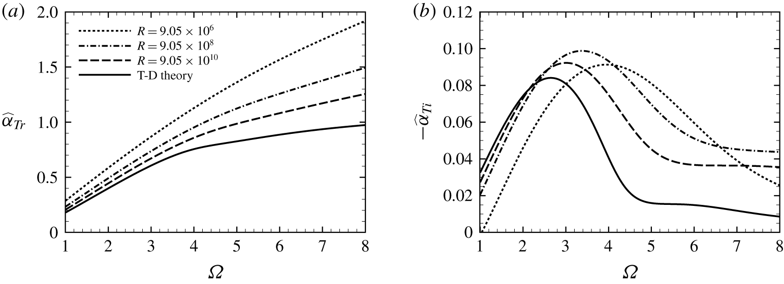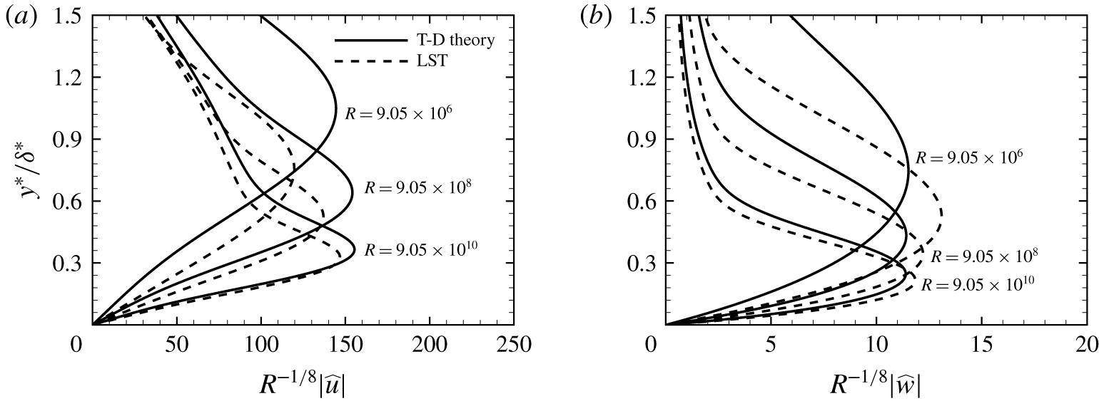


1 Introduction
Transition of boundary-layer flows from a laminar to turbulent state has been one of the most attractive and challenging problems in fluid mechanics. In an environment of weak disturbances, the path of transition consists of three stages: receptivity, linear eigenmode growth and nonlinear breakdown to turbulence (Morkovin Reference Morkovin1969; Kachanov Reference Kachanov1994; Wu Reference Wu2019). In the receptivity process, external perturbations (acoustic, vortical and entropy fluctuations in the free stream, and surface perturbations, e.g. roughness and gaps) excite instability modes of the boundary layer (Goldstein & Hultgren Reference Goldstein and Hultgren1989; Saric, Reed & Kerschen Reference Saric, Reed and Kerschen2002). Receptivity study aims to identify the mechanisms by which external perturbations excite instability modes, thereby determining the initial amplitudes and phases of the latter. The progress achieved in this field is due, to a large degree, to the studies based on the asymptotic analysis of the Navier–Stokes (N–S) equations at large Reynolds numbers (Goldstein & Hultgren Reference Goldstein and Hultgren1989). When dealing with generation of Tollmien–Schlichting (T–S) waves in boundary layers, this approach relies on the triple-deck theory, which is known to describe the lower-branch instability in the subsonic regime (Lin Reference Lin1946; Smith Reference Smith1979) and sufficiently oblique first Mack modes in the supersonic regime (Smith Reference Smith1989).
It was known from experimental observations (Laufer Reference Laufer1961; Schneider Reference Schneider2001) that acoustic noise influences significantly boundary-layer transition, most likely through the receptivity process. However, an acoustic wave cannot in general directly excite any instability mode because they have different dispersion relations. The characteristic wavelength of acoustic waves is typically much longer than that of any T–S mode, implying that the matching of the wavenumbers is not satisfied. For an acoustic wave to couple with a T–S wave, a scale-conversion mechanism is required. This crucial mechanism can be provided by surface roughness with a streamwise length scale comparable to that of T–S instability. The acoustic wave, whose frequency is taken to be in the characteristic range of the T–S wave, forces a so-called Stokes shear wave inside the boundary layer, which interacts with the roughness-induced mean-flow distortion, to excite a T–S mode. The asymptotic theory for this mechanism in subsonic boundary layers was formulated by Ruban (Reference Ruban1984) and Goldstein (Reference Goldstein1985). The roughness height  $h^{\ast }$ was assumed to be much smaller than the local boundary-layer thickness
 $\unicode[STIX]{x1D6FF}^{\ast }$, specifically
 $h^{\ast }\ll \unicode[STIX]{x1D6FF}^{\ast }R^{-1/8}$, so that a small distortion to the background flow is caused without altering the underlying instability to leading order, where
 $R$ is the Reynolds number based on the distance to the leading edge. Importantly, the theory shows that the amplitude of the T–S mode excited scales with
 $h^{\ast }$ as
 $(h^{\ast }/\unicode[STIX]{x1D6FF}^{\ast })R^{1/8}$ rather than
 $(h^{\ast }/\unicode[STIX]{x1D6FF}^{\ast })$ as one might expect without undertaking the asymptotic analysis. De Tullio & Ruban (Reference De Tullio and Ruban2015) carried out direct numerical simulations (DNS) to evaluate the asymptotic theory of receptivity for subsonic two-dimensional compressible boundary layers. Their results demonstrated that the theoretical solutions obtained for
 $R\gg 1$ hold at moderate Reynolds numbers; see also Mengaldo et al. (Reference Mengaldo, Kravtsova, Ruban and Sherwin2015), which confirmed that the roughness-induced mean flow is well predicted by triple-deck theory. An asymptotic theory for the receptivity of the boundary layer due to the interaction between vortical disturbances (representing free-stream turbulence) and a localized roughness element was presented by Duck, Ruban & Zhikharev (Reference Duck, Ruban and Zhikharev1996). They pointed out that, although a vortical disturbance does not penetrate into the boundary layer, it can interact with the roughness-induced steady perturbation at the outer edge of the boundary layer to generate a T–S mode. The theory of Duck et al. (Reference Duck, Ruban and Zhikharev1996) was extended by Wu (Reference Wu2001a) to allow for vortical disturbances with an arbitrary vertical distribution, thereby making it possible to compare the theoretical result with experimental data. Acoustic waves and vortical disturbances may each interact with distributed roughness of suitable frequency to excite stronger T–S waves than in the case of localized roughness elements (Wu Reference Wu2001b).
On the other hand, Zhigulev & Fedorov (Reference Zhigulev and Fedorov1987), Choudhari & Streett (Reference Choudhari and Streett1992) and Crouch (Reference Crouch1992) formulated receptivity theory in a finite-Reynolds-number framework, in which the steady and unsteady Orr–Sommerfeld (O–S) equations are used to describe the roughness-induced mean-flow distortion and instability, respectively. The instability mode excited is computed by solving an inhomogeneous unsteady O–S equation with the forcing generated by the interaction of the mean-flow distortion with an acoustic signature.
The boundary-layer receptivity mechanisms highlighted above have been studied and confirmed by experimental studies (e.g. Saric, Hoos & Radeztsky Reference Saric, Hoos, Radeztsky, Reda, Reed and Kobayashi1991; Zhou, Liu & Blackwelder Reference Zhou, Liu and Blackwelder1994; Dietz Reference Dietz1999; King & Breuer Reference King and Breuer2001; Würz et al. Reference Würz, Herr, Wörner, Rist, Wagner and Kachanov2003). Among these, Würz et al. (Reference Würz, Herr, Wörner, Rist, Wagner and Kachanov2003) conducted a joint experimental and DNS investigation of the generation of T–S waves in a boundary layer on an airfoil. They found that the scattering of acoustic waves by three-dimensional surface roughness is significantly stronger than that in the two-dimensional case; a similar observation was made by King & Breuer (Reference King and Breuer2001) in the case of a nominally flat-plate boundary layer.
Compared with subsonic flows, supersonic boundary-layer stability and receptivity exhibit new features (Fedorov Reference Fedorov2011; Zhong & Wang Reference Zhong and Wang2012). In a supersonic boundary layer, the dominant instability is the so-called first Mack mode up to a free-stream Mach number of approximately 4, and the second Mack mode for larger Mach numbers (Mack Reference Mack1984). Second modes have larger growth rates when two-dimensional, whereas first modes acquire their maximum growth rates when oblique. Second modes, and most first modes, are essentially inviscid, but lower-branch first modes are of a viscous nature and governed by the triple-deck structure when they are sufficiently three-dimensional with obliqueness angles  $\unicode[STIX]{x1D717}$ satisfying
 $\unicode[STIX]{x1D717}>\tan ^{-1}[(M^{2}-1)^{1/2}]$ (Smith Reference Smith1989), where
 $M$ is the local Mach number of the external stream. The receptivity of supersonic and hypersonic boundary layers becomes more complex than their subsonic counterparts. The generation of lower-branch first Mack modes is important because they are the first to be excited by external disturbances.
In order to understand receptivity to free-stream disturbances, Fedorov & Khokhlov (Reference Fedorov and Khokhlov1991, Reference Fedorov and Khokhlov2001) analysed the limiting behaviour of boundary-layer instability modes in the leading-edge region, and found that fast and slow modes are synchronized with fast and slow free-stream acoustic waves with the phase speeds  $1+1/M$ and
 $1-1/M$, respectively. Fedorov (Reference Fedorov2003a) showed that the former can be excited by the latter, respectively, through scattering or diffraction depending on the incident angle
 $\unicode[STIX]{x1D703}$. Unlike Lam–Rott asymptotic eigenmodes, the slow modes do not experience server decay, and hence the present receptivity to slow acoustic waves is much more efficient than the leading-edge adjustment mechanism in the subsonic case (Goldstein Reference Goldstein1983). Fast modes undergo decay and hence the receptivity to fast acoustic waves should be somewhat weaker. Fedorov (Reference Fedorov2003a) made a comparison with the experimental data of Maslov et al. (Reference Maslov, Shiplyuk, Sidorenko and Arnal2001), obtained in a Mach 6 wind tunnel for a flat plate with a sharp leading edge. Good agreement was observed for planar or moderately three-dimensional disturbances, but the prediction deteriorates and even exhibits opposite trends for larger obliqueness angles. Leading-edge receptivity mechanisms for modes with obliqueness angles close to, but smaller than,
 $\tan ^{-1}[(M^{2}-1)^{1/2}]$ were discussed by Goldstein & Ricco (Reference Goldstein and Ricco2018). The theory of Fedorov & Khokhlov (Reference Fedorov and Khokhlov1991, Reference Fedorov and Khokhlov2001), which is inviscid, ceases to be valid for highly oblique first modes that are of a viscous nature, have phase speeds much smaller than the free-stream velocity and acquire a triple-deck structure (Smith Reference Smith1989). These modes may be generated by acoustic or vortical disturbances interacting with local or distributed surface roughness. They may also be excited in the vicinity of their respective lower-branch neutral points by interactions between an acoustic wave and a vortical disturbance (Wu Reference Wu1999) or between two sound waves (Hernández & Wu Reference Hernández and Wu2019).
For supersonic and hypersonic boundary layers, shocks emerge and may play a relevant role in the receptivity because any of three elementary free-stream disturbances (representing acoustic waves, entropy and vortical fluctuations) interacts with the shock, generating all three downstream (see Duck, Lasseigne & Hussaini Reference Duck, Lasseigne and Hussaini1995, Reference Duck, Lasseigne and Hussaini1997; Maslov et al. Reference Maslov, Mironov, Kudryavtsev, Poplavskaya and Tsyryulnikov2010). DNS investigations of the receptivity of supersonic boundary layers to such disturbances have been carried out by Balakumar (Reference Balakumar2003, Reference Balakumar2005) and Ma & Zhong (Reference Ma and Zhong2003a,Reference Ma and Zhongb, Reference Ma and Zhong2005), among others. They found that free-stream slow and fast acoustic waves can excite first Mack modes and fast modes, respectively, as described by the theory of Fedorov & Khokhlov (Reference Fedorov and Khokhlov2001) and Fedorov (Reference Fedorov2003a). Vortical and entropy perturbations generate instability modes indirectly, namely, they first interact with the shock to generate slow or fast acoustic waves downstream, which then excite slow and fast instability modes. Simulations of the receptivity of the boundary layers over a parabola, blunt plates and cones have been carried out by Zhong (Reference Zhong2001), Zhong & Ma (Reference Zhong and Ma2006) and Balakumar (Reference Balakumar2006, Reference Balakumar2015), and the results indicate that bluntness reduces receptivity.
In the flows investigated by DNS mentioned above, shocks are sufficiently distant from the edge of the boundary layer that they do not influence directly the boundary-layer instability. Cowley & Hall (Reference Cowley and Hall1990) showed that, when a shock is close to the boundary layer, new instability modes arise, as occurs in the hypersonic boundary layer over a wedge with a small half-angle. Qin & Wu (Reference Qin and Wu2016) identified a new and rather unique receptivity mechanism for these modes. They found that any of three elementary types of free-stream disturbances (acoustic, vortical and entropy) with frequency and wavelength on the triple-deck scales interacts with the shock to generate a slow acoustic perturbation, which is reflected between the shock and the wall. In the vicinity of the lower-branch neutral curve, such a slow acoustic perturbation with suitable frequency and wavenumber is in exact resonance with a neutral eigenmode. As a result, the latter is excited directly by any single one alone of three elementary types of free-stream disturbance.
Receptivity mechanisms identified for subsonic boundary layers may continue to operate in the supersonic regime, but take different mathematical forms, and their effectiveness may differ significantly from that of their respective subsonic counterparts. In this paper, we shall consider such a case, which is the well-known mechanism of an acoustic wave interacting with a localized surface roughness (Ruban Reference Ruban1984; Goldstein Reference Goldstein1985). In the case of a subsonic boundary layer, the phase speed of any sound wave in the free stream is comparable with the free-stream velocity, and becomes infinite in the incompressible limit. It follows that, if the frequency of a sound wave is chosen to be comparable with the characteristic frequency of T–S instability, then its wavelength is necessarily much longer. In the case of a supersonic boundary layer, the majority of acoustic waves have phase speeds comparable with the free-stream velocity. The receptivity due to their interaction with surface roughness was studied by Choudhari & Kerschen (Reference Choudhari and Kerschen1990) and Fedorov (Reference Fedorov2003b) using finite-Reynolds-number theoretical approaches. The same mechanism was examined in the DNS of Balakumar (Reference Balakumar2005, Reference Balakumar2009), who found that this receptivity was rather weak in comparison with the leading-edge mechanism of Fedorov & Khokhlov (Reference Fedorov and Khokhlov2001) and Fedorov (Reference Fedorov2003a). A simple but significant fact is that, in the supersonic regime, there exists a subsect of free-stream acoustic waves whose frequencies and wavelengths are both comparable with those of the oblique first-mode instability, i.e. on the triple-deck scales, and the phase speeds are thus small. Such slowly propagating sound waves have the special property that a fluctuation with an  $O(\unicode[STIX]{x1D716}_{u})$ magnitude in the free stream generates in the boundary layer a much larger acoustic signature, characterized by
 $O(\unicode[STIX]{x1D716}_{u}R^{1/8})$ unsteady streamwise and spanwise velocities. Its interaction with the roughness-induced mean-flow distortion leads to much stronger receptivity than for acoustic waves not on the triple-deck scales. The present paper investigates this scenario using the high-Reynolds-number asymptotic approach, the triple-deck theory, which describes the impingement and reflection of the acoustic wave, the local mean-flow distortion caused by the roughness and, most importantly, their mutual interaction leading to excitation of a first Mack instability mode. Furthermore, DNS will be performed to provide, on the one hand, quantitative data, which are still lacking. On the other hand, the accuracy of the asymptotic theory will be assessed by quantitative comparisons between the theoretical and DNS results.
The rest of the paper is organized as follows. In § 2, the problem is to be formulated, the key non-dimensional parameters are introduced and relevant scalings specified. The set-up of DNS is described in § 3. In § 4, we present the asymptotic analysis of the receptivity process, and determine the ‘initial’ amplitude of the instability mode excited. The theoretical predictions are presented in § 5. In § 6, we describe the DNS results, and carry out rather detailed comparisons between the theoretical and numerical predictions. A summary and conclusions are given in § 7.
2 Problem statement and triple-deck scalings
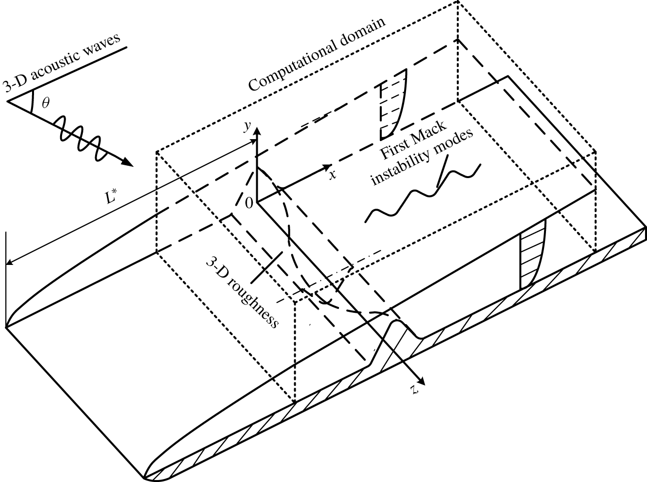
The physical model to be studied is a two-dimensional compressible boundary layer over a flat plate, on which an array of small-amplitude spanwise periodic, streamwise isolated roughness elements is located at a distance  $L^{\ast }$ downstream of the leading edge, as is depicted schematically in figure 1. The oncoming flow is a uniform stream with velocity
 $U_{\infty }$, through which a small-amplitude three-dimensional acoustic wave propagates and impinges on the boundary layer at an incident angle.
Schematic diagram of the interaction between three-dimensional (3-D) acoustic waves and three-dimensional roughness.

The flow physics involved is as follows. A three-dimensional acoustic wave, assumed to be originated from a distant source, propagates towards the boundary layer and is reflected, while at the same time it generates an unsteady viscous response within the boundary layer. Such a response will be referred to as an acoustic signature despite being rotational. On the other hand, the roughness induces a local mean-flow distortion. The steady and time-periodic perturbations interact with each other. The resulting disturbance is rather complex in the vicinity of the roughness, but evolves into a first-mode instability wave far downstream. We will study the excitation of these modes with sufficiently large spanwise wavenumbers using both triple-deck theory and DNS.
The flow is described in the Cartesian coordinate system  $(x^{\ast },y^{\ast },z^{\ast })$ with its origin being taken to be at the roughness site. The normalized space and time variables are
 $$\begin{eqnarray}(x,y,z)=(x^{\ast },y^{\ast },z^{\ast })/L^{\ast },\quad t=t^{\ast }U_{\infty }/L^{\ast }.\end{eqnarray}$$
The velocities in the streamwise, wall-normal and spanwise directions,  $(u^{\ast },v^{\ast },w^{\ast })$, the density
 $\unicode[STIX]{x1D70C}^{\ast }$, temperature
 $T^{\ast }$, pressure
 $p^{\ast }$ and dynamical viscosity
 $\unicode[STIX]{x1D707}^{\ast }$ are non-dimensionalized by their corresponding free-stream quantities, i.e.
 $$\begin{eqnarray}\left.\begin{array}{@{}c@{}}(u,v,w)=(u^{\ast },v^{\ast },w^{\ast })/U_{\infty },\quad \unicode[STIX]{x1D70C}=\unicode[STIX]{x1D70C}^{\ast }/\unicode[STIX]{x1D70C}_{\infty },\quad T=T^{\ast }/T_{\infty },\\ p=p^{\ast }/\unicode[STIX]{x1D70C}_{\infty }U_{\infty }^{2},\quad \unicode[STIX]{x1D707}=\unicode[STIX]{x1D707}^{\ast }/\unicode[STIX]{x1D707}_{\infty }.\end{array}\right\}\end{eqnarray}$$
Consistent with (2.1), the wavenumbers in the streamwise, wall-normal, spanwise directions,  $(\unicode[STIX]{x1D6FC}^{\ast },\unicode[STIX]{x1D6FE}^{\ast },\unicode[STIX]{x1D6FD}^{\ast })$, and frequency
 $\unicode[STIX]{x1D714}^{\ast }$ of a disturbance are normalized as
 $$\begin{eqnarray}(\unicode[STIX]{x1D6FC},\unicode[STIX]{x1D6FE},\unicode[STIX]{x1D6FD})=(\unicode[STIX]{x1D6FC}^{\ast },\unicode[STIX]{x1D6FE}^{\ast },\unicode[STIX]{x1D6FD}^{\ast })L^{\ast },\quad \unicode[STIX]{x1D714}=\unicode[STIX]{x1D714}^{\ast }L^{\ast }/U_{\infty }.\end{eqnarray}$$
The Mach number and the Reynolds number are defined as
 $$\begin{eqnarray}M=U_{\infty }/c_{\infty },\quad R=\unicode[STIX]{x1D70C}_{\infty }U_{\infty }L^{\ast }/\unicode[STIX]{x1D707}_{\infty },\end{eqnarray}$$
where  $c_{\infty }$ is the sound speed in the oncoming flow. Our focus will be on the supersonic case with
 $M>1$, and for theoretical development we take
 $R\gg 1$.
The DNS of the receptivity will be carried out guided by the asymptotic analysis. The latter is based on the triple-deck theory, which describes the first-mode instability in a supersonic boundary layer (Smith Reference Smith1989). These instability waves must be sufficiently three-dimensional with their spanwise and streamwise wavenumbers,  $\unicode[STIX]{x1D6FD}_{T}$ and
 $\unicode[STIX]{x1D6FC}_{T}$, satisfying
 $\unicode[STIX]{x1D6FD}_{T}>\sqrt{M^{2}-1}\unicode[STIX]{x1D6FC}_{T}$. For a free-stream acoustic wave to excite a lower-branch instability mode, its frequency has to match that of the latter, which is of
 $O(R^{1/4})$. Of particular interest are acoustic waves with
 $O(R^{-3/8})$ wavelength, which is on the triple-deck scale as well, and since their phase velocity
 $c_{s}=O(R^{-1/8})$, they will be referred to as slow acoustic waves. The induced signature in the boundary layer is amplified by the background shear flow, and is described by the interactive structure of the triple deck, as opposed to the passive Stokes layer for conventional sound waves. A similar feature was noted for gravity waves on the triple-deck scales in a stratified boundary layer (Wu & Zhang Reference Wu and Zhang2008).
Acoustic waves and instability modes satisfy their own dispersion relations, and therefore, despite the fact that they are both on the triple-deck scales, a roughness is still required in order to achieve the precise scale matching required for their coupling. Its streamwise length scale must be of  $O(R^{-3/8})$. According to the triple-deck formalism, the flow near the wall roughness is divided into three regions in the wall-normal direction, and the wall roughness should be contained within the lower deck, that is, its height
 $h^{\ast }$ must be
 $O(R^{-5/8}L^{\ast })$ or smaller. When
 $h^{\ast }=O(R^{-5/8}L^{\ast })$, the induced mean-flow distortion is fully nonlinear. The study by Mengaldo et al. (Reference Mengaldo, Kravtsova, Ruban and Sherwin2015) in the subsonic regime demonstrated that the prediction by triple-deck theory agreed rather well with DNS at moderate Reynolds numbers even when flow separation occurs. In this paper, we shall assume that
 $h^{\ast }\ll R^{-5/8}L^{\ast }$ and the acoustic disturbance amplitude
 $\unicode[STIX]{x1D716}_{u}\ll R^{-1/4}$, for which the system can be linearized and solved analytically.
3 Direct numerical simulations
3.1 The governing equations
The dimensionless compressible N–S equations that govern the flow field ( $u,v,w,p,\unicode[STIX]{x1D70C}$,
 $T$) (see (2.2)) are written in the conservative form,
 $$\begin{eqnarray}\frac{\unicode[STIX]{x2202}\boldsymbol{U}}{\unicode[STIX]{x2202}t}+\frac{\unicode[STIX]{x2202}\boldsymbol{E}}{\unicode[STIX]{x2202}x}+\frac{\unicode[STIX]{x2202}\boldsymbol{F}}{\unicode[STIX]{x2202}y}+\frac{\unicode[STIX]{x2202}\boldsymbol{G}}{\unicode[STIX]{x2202}z}+\boldsymbol{B}=\frac{\unicode[STIX]{x2202}\boldsymbol{E}_{v}}{\unicode[STIX]{x2202}x}+\frac{\unicode[STIX]{x2202}\boldsymbol{F}_{v}}{\unicode[STIX]{x2202}y}+\frac{\unicode[STIX]{x2202}\boldsymbol{G}_{v}}{\unicode[STIX]{x2202}z},\end{eqnarray}$$
where  $\boldsymbol{U}$ is the conservative flux,
 $\boldsymbol{E}$,
 $\boldsymbol{F}$ and
 $\boldsymbol{G}$ are the nonlinear terms,
 $\boldsymbol{E}_{v}$,
 $\boldsymbol{F}_{v}$ and
 $\boldsymbol{G}_{v}$ are the viscosity terms and
 $\boldsymbol{B}$ is a body force, introduced to render the base flow
 $\boldsymbol{U}_{B}$ (Blasius solution) to satisfy (3.1); the expression for each term can be found in Qin & Dong (Reference Qin and Dong2016).
Before the system (3.1) can be discretized and solved, it is necessary to calculate the unperturbed base flow, specify the free-stream disturbance, and to set up boundary conditions as well as the inflow and outflow conditions; these will be done in §§ 3.2–3.5. The simulation of receptivity is to be carried out using the Blasius solution as the base flow. Since the length scale of the roughness-induced distortion is  $O(R^{-3/8}L^{\ast })$, much shorter than the scale on which the Blasius flow develops, we neglect the non-parallel effect of the Blasius solution in order to focus on the roughness-induced receptivity.
The inflow condition is imposed as a superposition of the Blasius solution and a small-amplitude acoustic signature. The boundary conditions at the perturbed wall surface are to be approximated by the equivalent ones at the flat plate via the first-order Taylor expansion. The total flow field can be decomposed into a steady base flow and perturbation, namely,
 $$\begin{eqnarray}\displaystyle & & \displaystyle [u,v,w,\unicode[STIX]{x1D70C},T,p](x,y,z,t)\nonumber\\ \displaystyle & & \displaystyle \quad =[U_{B},0,0,R_{B},T_{B},P_{B}](y)+\frac{\unicode[STIX]{x1D716}_{u}}{2}[\widetilde{u}(y),\widetilde{v}(y),\widetilde{w}(y),\widetilde{\unicode[STIX]{x1D70C}}(y),\widetilde{T}(y),\widetilde{p}(y)]\text{e}^{\text{i}(\unicode[STIX]{x1D6FC}_{s}x+\unicode[STIX]{x1D6FD}_{s}z-\unicode[STIX]{x1D714}t)}\nonumber\\ \displaystyle & & \displaystyle \qquad +\,[U_{h},V_{h},W_{h},R_{h},T_{h},P_{h}](x,y,z)+[\widehat{u},\widehat{v},\widehat{w},\widehat{\unicode[STIX]{x1D70C}},\widehat{T},\widehat{p}](x,y,z,t)+\text{c.c.},\end{eqnarray}$$
where  $[U_{B},0,0,R_{B},T_{B},P_{B}]$ denotes the Blasius solution,
 $[\widetilde{u},\widetilde{v},\widetilde{w},\widetilde{\unicode[STIX]{x1D70C}},\widetilde{T},\widetilde{p}]$ stands for the response of the boundary layer to the free-stream sound over a smooth flat plate, with
 $\unicode[STIX]{x1D716}_{u}$ being the amplitude of the incident acoustic wave,
 $\unicode[STIX]{x1D6FC}_{s}$ and
 $\unicode[STIX]{x1D6FD}_{s}$ its streamwise and spanwise wavenumbers, respectively;
 $[U_{h},V_{h},W_{h},R_{h},T_{h},P_{h}]$ represents the localized mean-flow distortion induced by the surface roughness. The interaction of the acoustic signature with the mean-flow distortion produces the scattered field
 $[\widehat{u},\widehat{v},\widehat{w},\widehat{\unicode[STIX]{x1D70C}},\widehat{T},\widehat{p}]$, from which an instability mode emerges.
3.2 Blasius solution
In this subsection, we consider  $[U_{B},V_{B},0,R_{B},T_{B},P_{B}]$ in (3.2). The base flow over a smooth flat plate is governed by the classical compressible boundary-layer equations.
We introduce the Dorodnitsyn–Howarth transformation,
 $$\begin{eqnarray}\unicode[STIX]{x1D709}=(1+x),\quad \unicode[STIX]{x1D702}=\sqrt{\frac{R}{2(1+x)}}\int _{0}^{y}R_{B}\,\text{d}y.\end{eqnarray}$$
In terms of  $\unicode[STIX]{x1D709}$ and
 $\unicode[STIX]{x1D702}$, the solution can be expressed in the self-similar form,
 $$\begin{eqnarray}\left.\begin{array}{@{}c@{}}\displaystyle U_{B}(\unicode[STIX]{x1D702})=f^{\prime }(\unicode[STIX]{x1D702}),\quad V_{B}=-\sqrt{\frac{1}{2\unicode[STIX]{x1D709}R}}\left[f(\unicode[STIX]{x1D702})g(\unicode[STIX]{x1D702})-f^{\prime }(\unicode[STIX]{x1D702})\int _{0}^{\unicode[STIX]{x1D702}}g(\unicode[STIX]{x1D702})\,\text{d}\unicode[STIX]{x1D702}\right],\\ \displaystyle T_{B}(\unicode[STIX]{x1D702})=g(\unicode[STIX]{x1D702}),\quad P_{B}(\unicode[STIX]{x1D702})=\frac{1}{\unicode[STIX]{x1D6FE}M^{2}},\quad R_{B}(\unicode[STIX]{x1D702})=\frac{1}{g(\unicode[STIX]{x1D702})},\end{array}\right\}\end{eqnarray}$$
where  $f$ and
 $g$ satisfy the coupled equations,
 $$\begin{eqnarray}(Cf^{\prime \prime })^{\prime }+ff^{\prime \prime }=0,\quad (Cg^{\prime })^{\prime }+P_{r}fg^{\prime }+(\unicode[STIX]{x1D6FE}-1)M^{2}P_{r}C{f^{\prime \prime }}^{2}=0;\end{eqnarray}$$
here,  $C(\unicode[STIX]{x1D702})=\unicode[STIX]{x1D707}_{B}/T_{B}=T_{B}^{1/2}(1+110.4/T_{\infty })/(T_{B}+110.4/T_{\infty })$ when Sutherland’s law is used, the Prandtl number
 $Pr$ is a constant and equals 0.72 and
 $\unicode[STIX]{x1D6FE}=1.4$ is the ratio of the specific heats. Equation (3.5a,b) is subject to the boundary conditions,
 $$\begin{eqnarray}f^{\prime }(0)=0,\quad g(0)=T_{w};\quad f^{\prime },\quad g\rightarrow 1\quad \text{as}~\unicode[STIX]{x1D702}\rightarrow \infty .\end{eqnarray}$$
In this work, we take the wall temperature  $T_{w}$ to be
 $$\begin{eqnarray}T_{w}=1+\sqrt{Pr}(\unicode[STIX]{x1D6FE}-1)M^{2}/2,\end{eqnarray}$$
which is the temperature of an adiabatic wall if  $P_{r}=1$, but only approximately so if
 $P_{r}\neq 1$, e.g.
 $P_{r}=0.72$, the value that we shall use. The displacement thickness
 $\unicode[STIX]{x1D6FF}^{\ast }$ is expressed as
 $$\begin{eqnarray}\unicode[STIX]{x1D6FF}^{\ast }=\int _{0}^{\infty }(1-R_{B}U_{B})\,\text{d}y^{\ast }=\sqrt{2}L^{\ast }R^{-1/2}\int _{0}^{\infty }[g(\unicode[STIX]{x1D702})-f^{\prime }(\unicode[STIX]{x1D702})]\,\text{d}\unicode[STIX]{x1D702}.\end{eqnarray}$$
3.3 Inflow boundary condition: response to free-stream acoustic disturbances and continuous spectrum of the Orr–Sommerfeld equation
In this subsection, we consider the acoustic signature in the boundary layer, represented by the  $O(\unicode[STIX]{x1D716}_{u})$ term in (3.2). With the parallel-flow assumption, the non-dimensional base flow can be viewed as a function of
 $y$ only, with the dependence on
 $x$ becoming parametric. The disturbance satisfies the linearized continuity, momentum, energy and state equations. If we introduce
 $\unicode[STIX]{x1D753}$ as
 $$\begin{eqnarray}\unicode[STIX]{x1D753}(y)=\left(\widetilde{u},\frac{\text{d}\widetilde{u}}{\text{d}y},\widetilde{v},\widetilde{p},\widetilde{T},\frac{\text{d}\widetilde{T}}{\text{d}y},\widetilde{w},\frac{\text{d}\widetilde{w}}{\text{d}y}\right)^{T},\end{eqnarray}$$
then  $\unicode[STIX]{x1D753}$ is governed by a system of first-order equations,
 $$\begin{eqnarray}\frac{\text{d}\unicode[STIX]{x1D753}}{\text{d}y}=\unicode[STIX]{x1D63F}(y)\unicode[STIX]{x1D753},\end{eqnarray}$$
where  $\unicode[STIX]{x1D63F}$ is an
 $8\times 8$ matrix, whose expression can be found in Malik (Reference Malik1990).
At a finite Reynolds number, the incident sound wave and the signature induced in the boundary layer correspond to the acoustic branch of the continuous modes of the system (3.10). With allowance for the presence of continuous modes, the far-field asymptotic behaviour of  $\unicode[STIX]{x1D753}$ can be written as
 $$\begin{eqnarray}\unicode[STIX]{x1D753}=\mathop{\sum }_{i=1}^{8}A_{i}\unicode[STIX]{x1D743}_{i}\text{e}^{\unicode[STIX]{x1D706}_{i}y}\quad \text{as}~y\rightarrow \infty ,\end{eqnarray}$$
where  $\unicode[STIX]{x1D706}_{i}$ and
 $\unicode[STIX]{x1D743}_{i}$ are the eigenvalues and eigenvectors of the matrix
 $\unicode[STIX]{x1D63F}_{\infty }\equiv \lim _{y\rightarrow \infty }\unicode[STIX]{x1D63F}$, respectively, and
 $A_{i}$ represents the coefficient of each component. The eigenvalues are given in Balakumar & Malik (Reference Balakumar and Malik1992). The continuous mode shape is oscillatory in the free stream, and so some of the eigenvalues
 $\unicode[STIX]{x1D706}_{i}$ must be (almost) purely imaginary with
 $R\gg 1$. The dispersion relationship can be written as
 $\unicode[STIX]{x1D6FC}_{s}=\unicode[STIX]{x1D6FC}_{s}(\unicode[STIX]{x1D714},\unicode[STIX]{x1D6FE}_{s},\unicode[STIX]{x1D6FD}_{s})$, and for a spatially developing wave
 $\unicode[STIX]{x1D6FE}_{s}$,
 $\unicode[STIX]{x1D6FD}_{s}$ and
 $\unicode[STIX]{x1D714}$ are real, and
 $\unicode[STIX]{x1D6FC}_{s}$ is complex, whose imaginary part is
 $O(R^{-1})$. The imaginary part of
 $\unicode[STIX]{x1D6FC}_{s}$ is positive because continuous modes are decaying perturbations.
For an acoustic wave, we take  $\unicode[STIX]{x1D706}_{5}=-\unicode[STIX]{x1D706}_{6}=\text{i}\unicode[STIX]{x1D6FE}_{s}$. In the limit of large Reynolds number,
 $R\gg 1$, the dispersion relationship to leading-order accuracy is
 $$\begin{eqnarray}-(\unicode[STIX]{x1D6FC}_{s}-\unicode[STIX]{x1D714})^{2}M^{2}+\unicode[STIX]{x1D6FC}_{s}^{2}+\unicode[STIX]{x1D6FE}_{s}^{2}+\unicode[STIX]{x1D6FD}_{s}^{2}=0,\end{eqnarray}$$
from which it follows
 $$\begin{eqnarray}\unicode[STIX]{x1D6FC}_{s}=\frac{M^{2}\unicode[STIX]{x1D714}\pm \sqrt{M^{2}\unicode[STIX]{x1D714}^{2}+(M^{2}-1)(\unicode[STIX]{x1D6FE}_{s}^{2}+\unicode[STIX]{x1D6FD}_{s}^{2})}}{M^{2}-1}.\end{eqnarray}$$
The incident angle is defined as
 $$\begin{eqnarray}\unicode[STIX]{x1D703}=\cos ^{-1}\frac{\unicode[STIX]{x1D6FC}_{s}}{\sqrt{\unicode[STIX]{x1D6FC}_{s}^{2}+\unicode[STIX]{x1D6FD}_{s}^{2}+\unicode[STIX]{x1D6FE}_{s}^{2}}}.\end{eqnarray}$$
Without loss of generality, we take  $\unicode[STIX]{x1D714}>0$. If the ‘+’ sign in (3.13) is selected, the phase speed is
 $$\begin{eqnarray}c_{s}=\frac{\unicode[STIX]{x1D714}}{\unicode[STIX]{x1D6FC}_{s}}=1-\frac{1}{M\cos \unicode[STIX]{x1D703}},\quad \unicode[STIX]{x1D703}\in \left[0,\cos ^{-1}\frac{1}{M}\right),\end{eqnarray}$$
for which  $c_{s}>0$ and
 $\unicode[STIX]{x1D6FC}_{s}>0$. Since
 $c_{s}$ is smaller than the speed of the oncoming stream, this disturbance is referred to as a slow acoustic wave. On the other hand, if the ‘-’ sign in (3.13) is selected, the phase speed
 $c_{s}=1+1/(M\cos \unicode[STIX]{x1D703})$ can be either greater than 1 or negative, depending on the incident angle: the disturbance corresponds to a fast acoustic wave for
 $\unicode[STIX]{x1D703}\in [0,\unicode[STIX]{x03C0}/2)$, but to a slow acoustic wave for
 $\unicode[STIX]{x1D703}\in (\unicode[STIX]{x03C0}+\cos ^{-1}(1/M),3\unicode[STIX]{x03C0}/2)$. Therefore, in addition to (3.15), there also exist slow acoustic waves having phase speeds
 $$\begin{eqnarray}c_{s}=\frac{\unicode[STIX]{x1D714}}{\unicode[STIX]{x1D6FC}_{s}}=1+\frac{1}{M\cos \unicode[STIX]{x1D703}},\quad \unicode[STIX]{x1D703}\in \left(\unicode[STIX]{x03C0}+\cos ^{-1}\frac{1}{M},\frac{3\unicode[STIX]{x03C0}}{2}\right),\end{eqnarray}$$
for which  $c_{s}<0$ and
 $\unicode[STIX]{x1D6FC}_{s}<0$. Note that for both the cases mentioned above, the group velocity satisfies
 $\text{d}\unicode[STIX]{x1D714}/\text{d}\unicode[STIX]{x1D6FC}_{s}=1\mp \cos \unicode[STIX]{x1D703}/M>0$.
Let matrix  $\unicode[STIX]{x1D641}=[\unicode[STIX]{x1D743}_{1},\unicode[STIX]{x1D743}_{2},\unicode[STIX]{x1D743}_{3},\unicode[STIX]{x1D743}_{4},\unicode[STIX]{x1D743}_{5},\unicode[STIX]{x1D743}_{6},\unicode[STIX]{x1D743}_{7},\unicode[STIX]{x1D743}_{8}]$, or in terms their components
 $\unicode[STIX]{x1D60D}_{ji}=\unicode[STIX]{x1D709}_{ji}$, and let
 $\unicode[STIX]{x1D641}^{-1}$ be its inverse. Then
 $A_{i}$ can be expressed as
 $$\begin{eqnarray}A_{i}=\left(\mathop{\sum }_{j=1}^{8}\unicode[STIX]{x1D60D}_{ij}^{-1}\unicode[STIX]{x1D719}_{j}\right)\text{e}^{-\unicode[STIX]{x1D706}_{i}y}\quad \text{as}~y\rightarrow \infty \quad (i=1,2\ldots 8).\end{eqnarray}$$
The real parts of  $\unicode[STIX]{x1D706}_{2}$,
 $\unicode[STIX]{x1D706}_{4}$ and
 $\unicode[STIX]{x1D706}_{8}$ are positive, and so in order to render the solution bounded,
 $A_{2},A_{4},A_{8}$ must be set to zero. For
 $\unicode[STIX]{x1D6FC}_{s}>0$ (
 $c_{s}>0$), the incident acoustic wave corresponds to
 $\unicode[STIX]{x1D706}_{5}=\text{i}\unicode[STIX]{x1D6FE}_{s}$ as it has a negative vertical group velocity, whereas the computed
 $A_{6}\unicode[STIX]{x1D709}_{16}$ represents the amplitude of the acoustic wave reflected by the boundary layer. In this work,
 $[\widetilde{u}(y),\widetilde{v}(y),\widetilde{w}(y),\widetilde{\unicode[STIX]{x1D70C}}(y),\widetilde{T}(y),\widetilde{p}(y)]$ are normalized such that the streamwise velocity amplitude of the incident acoustic wave is unity, i.e.
 $A_{5}\unicode[STIX]{x1D709}_{15}=1$. Thus, the full boundary conditions for continuous modes are
 $$\begin{eqnarray}\left.\begin{array}{@{}c@{}}\displaystyle \widetilde{u}(0)=\widetilde{v}(0)=\widetilde{w}(0)=\widetilde{T}(0)=0\quad \text{at}~y=0,\\ \displaystyle \mathop{\sum }_{j=1}^{8}F_{2j}^{-1}\unicode[STIX]{x1D719}_{j}=0,\quad \!\mathop{\sum }_{j=1}^{8}F_{4j}^{-1}\unicode[STIX]{x1D719}_{j}=0,\quad \!\mathop{\sum }_{j=1}^{8}F_{8j}^{-1}\unicode[STIX]{x1D719}_{j}=0,\quad \!\mathop{\sum }_{j=1}^{8}F_{5j}^{-1}\unicode[STIX]{x1D719}_{j}\text{e}^{-\unicode[STIX]{x1D706}_{5}y}=\frac{1}{\unicode[STIX]{x1D709}_{15}}\quad \text{as}~y\rightarrow \infty .\end{array}\right\}\end{eqnarray}$$
The reflection coefficient is defined as the ratio of the amplitude of the reflected acoustic wave to that of the incident, i.e.
 $$\begin{eqnarray}\mathscr{R}=A_{6}\unicode[STIX]{x1D709}_{16}.\end{eqnarray}$$
In the case of  $\unicode[STIX]{x1D6FC}_{s}<0$ (
 $c_{s}<0$), the roles of
 $A_{5}$ and
 $A_{6}$ are exchanged. Thus, the streamwise velocity in the free stream is expressed as
 $$\begin{eqnarray}\left.\begin{array}{@{}c@{}}\displaystyle \widetilde{u}(y)=\text{e}^{\text{i}\unicode[STIX]{x1D6FE}_{s}y}+\mathscr{R}\text{e}^{-\text{i}\unicode[STIX]{x1D6FE}_{s}y}\quad \text{for}~\unicode[STIX]{x1D6FC}_{s}>0,\\ \displaystyle \widetilde{u}(y)=\text{e}^{-\text{i}\unicode[STIX]{x1D6FE}_{s}y}+\mathscr{R}\text{e}^{\text{i}\unicode[STIX]{x1D6FE}_{s}y}\quad \text{for}~\unicode[STIX]{x1D6FC}_{s}<0,\end{array}\right\}\end{eqnarray}$$
where  $\unicode[STIX]{x1D6FE}_{s}>0$.
3.4 Wall boundary conditions
The no-slip and isothermal boundary conditions are imposed at the roughness surface, and so the total velocity and temperature field at the surface are given as
 $$\begin{eqnarray}[u,v,w,T](x,h(x,z),z,t)=[0,0,0,T_{w}],\end{eqnarray}$$
where  $h(x,z)=h^{\ast }(x,z)/L^{\ast }$ is the normalized shape function of the roughness. Calculations will be performed for a roughness array which is spanwise periodic and streamwise localized with a Gaussian shape,
 $$\begin{eqnarray}h(x,z)=h_{0}\text{e}^{-x^{2}/d^{2}}\cos (\unicode[STIX]{x1D6FD}_{w}z),\end{eqnarray}$$
where  $d$ and
 $h_{0}$ are dimensionless measures of the roughness width and height respectively, and
 $\unicode[STIX]{x1D6FD}_{w}$ the spanwise wavenumber. Applying the first-order Taylor expansion to (3.21) for
 $h\ll 1$, we obtain the approximate boundary conditions,
 $$\begin{eqnarray}[u,v,w,T]+h\left[\frac{\unicode[STIX]{x2202}u}{\unicode[STIX]{x2202}y},\frac{\unicode[STIX]{x2202}v}{\unicode[STIX]{x2202}y},\frac{\unicode[STIX]{x2202}w}{\unicode[STIX]{x2202}y},\frac{\unicode[STIX]{x2202}T}{\unicode[STIX]{x2202}y}\right]=[0,0,0,T_{w}]\quad \text{at}~y=0,\end{eqnarray}$$
which is of the mixed type. If the first two terms in (3.2) are used in (3.23), there follows, to leading-order accuracy, the Dirichlet boundary conditions,
 $$\begin{eqnarray}\left.\begin{array}{@{}c@{}}\displaystyle u+h\frac{\unicode[STIX]{x2202}U_{B}}{\unicode[STIX]{x2202}y}+\frac{\unicode[STIX]{x1D716}_{u}}{2}h\frac{\unicode[STIX]{x2202}\widetilde{u}}{\unicode[STIX]{x2202}y}\text{e}^{\text{i}[\unicode[STIX]{x1D6FC}_{s}(x-x_{0})+\unicode[STIX]{x1D6FD}_{s}z-\unicode[STIX]{x1D714}t]}+\text{c.c.}=0,\\ \displaystyle v+\frac{\unicode[STIX]{x1D716}_{u}}{2}h\frac{\unicode[STIX]{x2202}\widetilde{v}}{\unicode[STIX]{x2202}y}\text{e}^{\text{i}[\unicode[STIX]{x1D6FC}_{s}(x-x_{0})+\unicode[STIX]{x1D6FD}_{s}z-\unicode[STIX]{x1D714}t]}+\text{c.c.}=0,\\ \displaystyle w+\frac{\unicode[STIX]{x1D716}_{u}}{2}h\frac{\unicode[STIX]{x2202}\widetilde{w}}{\unicode[STIX]{x2202}y}\text{e}^{\text{i}[\unicode[STIX]{x1D6FC}_{s}(x-x_{0})+\unicode[STIX]{x1D6FD}_{s}z-\unicode[STIX]{x1D714}t]}+\text{c.c.}=0,\\ \displaystyle T+h\frac{\unicode[STIX]{x2202}T_{B}}{\unicode[STIX]{x2202}y}+\frac{\unicode[STIX]{x1D716}_{u}}{2}h\frac{\unicode[STIX]{x2202}\widetilde{T}}{\unicode[STIX]{x2202}y}\text{e}^{\text{i}[\unicode[STIX]{x1D6FC}_{s}(x-x_{0})+\unicode[STIX]{x1D6FD}_{s}z-\unicode[STIX]{x1D714}t]}+\text{c.c.}=T_{w},\end{array}\right\}\end{eqnarray}$$
where  $x_{0}$ represents the streamwise coordinate of the inlet. Note that the flow field represents the mean flow induced by the wall roughness when
 $\unicode[STIX]{x1D716}_{u}=0$. Use of either boundary conditions (3.23) or (3.24) allows both the mean-flow distortion and the acoustic signature to be computed in the DNS.
3.5 Outflow and upper boundary conditions
A buffer region is imposed as the outflow condition downstream so that the waves will not be reflected back into the computational domain. The Navier–Stokes characteristic boundary condition (NSCBC; see Poinsot & Lele Reference Poinsot and Lele1992) is employed at the upper boundary, i.e. for the outgoing wave, its values at the boundary are extrapolated using the information at interior points, while the boundary values of the incoming wave are specified as the incident free-stream acoustic disturbance.
3.6 Discretization
With the boundary conditions now being specified on the flat surface, we discretize (3.1) on a chosen cubic domain,  $x_{l}^{\ast }/\unicode[STIX]{x1D6FF}^{\ast }\times y_{l}^{\ast }/\unicode[STIX]{x1D6FF}^{\ast }\times z_{l}^{\ast }/\unicode[STIX]{x1D6FF}^{\ast }$, and denote each grid by
 $(x_{i},y_{j},z_{k})$ with
 $i\in [0,In]$,
 $j\in [0,Jn]$ and
 $k\in [0,Kn]$. Uniform grids are employed in both the streamwise and spanwise directions, while non-uniform grids clustered in the near-wall region are used in the wall-normal direction.
The nonlinear terms are discretized by using the fifth-order finite-difference scheme with flux splitting according to positive and negative eigenvalues of the Jacobian matrix, while the viscous terms are discretized by the sixth-order central difference scheme. The second-order Runge–Kutta method is used for time evolution. The schemes and the method to generate the wall-normal grids are described in Qin & Dong (Reference Qin and Dong2016).
3.7 Receptivity coefficient
In this section, we consider the scattered field  $[\widehat{u},\widehat{v},\widehat{w},\widehat{\unicode[STIX]{x1D70C}},\widehat{T},\widehat{p}]$ in (3.2). The DNS give the total flow field, from which the pre-calculated base flow, the roughness-induced local mean-flow distortion and the acoustic signature are subtracted out to obtain the scattered signature. A main aim of studying receptivity is to determine the amplitude of the instability mode excited in terms of external disturbances, presently, the free-stream acoustic wave and the surface roughness. Since the disturbance is complex near the roughness, the modal amplitude can only be defined by considering the asymptotic behaviour of the scattered field sufficiently downstream, where the mode emerges and amplifies exponentially, e.g. the streamwise velocity
 $\widehat{u}(x,y,z,t)$ behaves as
 $$\begin{eqnarray}|\widehat{u}|\equiv \max _{y,z,t}(|\widehat{u}(x,y,z,t)|)\sim \text{e}^{-\unicode[STIX]{x1D6FC}_{Ti}x};\end{eqnarray}$$
where here the modal growth rate  $-\unicode[STIX]{x1D6FC}_{Ti}$ is independent of
 $x$ since we have neglected the non-parallelism of the base flow over a flat wall. We introduce the concept of ‘equivalent amplitude’, namely, the amplitude of the mode at the roughness site (
 $x=0$) whose downstream evolution is the same as that of the disturbance excited (Wu Reference Wu2001a). In this sense, the equivalent amplitude of the streamwise velocity can be defined as
 $$\begin{eqnarray}A_{u0}\equiv \lim _{x\rightarrow \infty }\max _{y,z,t}|\widehat{u}(x,y,z)|\text{e}^{\unicode[STIX]{x1D6FC}_{Ti}x}.\end{eqnarray}$$
This equivalent amplitude is what is customarily referred to as the ‘initial amplitude’. The receptivity coefficient is defined as the ratio of the streamwise-velocity amplitude of the excited instability mode to that of the incident acoustic wave,
 $$\begin{eqnarray}{\mathcal{K}}=A_{u0}/\unicode[STIX]{x1D716}_{u}.\end{eqnarray}$$
4 Triple-deck theory for acoustic–roughness interaction
As stated in § 2, the frequency and wavelength of the oncoming acoustic waves are assumed to be comparable with those of lower-branch instability modes, which are of  $O(R^{1/4})$ and
 $O(R^{-3/8})$, respectively. Correspondingly, the phase speed is
 $c_{s}=O(R^{-1/8})$, which requires the incident angle to be within an
 $O(R^{-1/8})$ vicinity of
 $\cos ^{-1}(1/M)$ if
 $c_{s}>0$, or of
 $(\unicode[STIX]{x03C0}+\cos ^{-1}(1/M))$ if
 $c_{s}<0$, according to (3.15) and (3.16). Receptivity due to the interactions between two such slow sound waves, or between one such wave and distributed surface roughness, was considered by Hernández & Wu (Reference Hernández and Wu2019). Here, we analyse the receptivity due to its interaction with streamwise isolated roughness, whose horizontal length scale is also of
 $O(R^{-3/8})$. The acoustic signature and the roughness-induced mean flow are both described by the standard triple-deck structure (Smith Reference Smith1973; Stewartson Reference Stewartson1974; Smith, Sykes & Brighton Reference Smith, Sykes and Brighton1977), and so is the interaction between them. The rescaled streamwise and spanwise coordinates and the time variable are introduced as
 $$\begin{eqnarray}\left.\begin{array}{@{}c@{}}\displaystyle (x,z)=\unicode[STIX]{x1D706}^{-5/4}(M^{2}-1)^{-3/8}C^{3/8}T_{w}^{3/2}\unicode[STIX]{x1D716}^{3}(X,Z),\\ \displaystyle t=\unicode[STIX]{x1D706}^{-3/2}(M^{2}-1)^{-1/4}C^{1/4}T_{w}\unicode[STIX]{x1D716}^{2}\widehat{t},\end{array}\right\}\end{eqnarray}$$
where  $\unicode[STIX]{x1D716}=R^{-1/8}$ is a small parameter,
 $T_{w}$ the wall temperature given by (3.7), the constant
 $C=T_{w}^{1/2}(1+110.4/T_{\infty })/(T_{w}+110.4/T_{\infty })$ and
 $\unicode[STIX]{x1D706}=C^{1/2}f^{\prime \prime }(0)/\sqrt{2}$ is the wall shear of the Blasius profile with
 $f^{\prime \prime }(0)$ being obtained by solving (3.5a,b)–(3.6) numerically.
The streamwise and spanwise wavenumbers and frequency of the disturbance scale accordingly as
 $$\begin{eqnarray}\left.\begin{array}{@{}c@{}}(\widehat{\unicode[STIX]{x1D6FC}},\widehat{\unicode[STIX]{x1D6FD}})=\unicode[STIX]{x1D706}^{-5/4}(M^{2}-1)^{-3/8}C^{3/8}T_{w}^{3/2}\unicode[STIX]{x1D716}^{3}(\unicode[STIX]{x1D6FC},\unicode[STIX]{x1D6FD}),\\ \unicode[STIX]{x1D6FA}=\unicode[STIX]{x1D706}^{-3/2}(M^{2}-1)^{-1/4}C^{1/4}T_{w}\unicode[STIX]{x1D716}^{2}\unicode[STIX]{x1D714}.\end{array}\right\}\end{eqnarray}$$
In the lower deck, the rescaled normal coordinate is introduced by writing
 $$\begin{eqnarray}y=\unicode[STIX]{x1D706}^{-3/4}(M^{2}-1)^{-1/8}C^{5/8}T_{w}^{3/2}\unicode[STIX]{x1D716}^{5}Y.\end{eqnarray}$$
The roughness is spanwise periodic, and its shape in the streamwise direction can be specified as a function of  $X$,
 $$\begin{eqnarray}Y=HF(X)\text{e}^{\text{i}\widehat{\unicode[STIX]{x1D6FD}}_{w}Z}+\text{c.c.},\end{eqnarray}$$
where
 $$\begin{eqnarray}F(X)=\text{e}^{-X^{2}/\widehat{d}^{2}},\end{eqnarray}$$
with  $\widehat{d}$ being a measuring of the roughness width.
The dominant interaction between the roughness and the acoustic wave takes place in the lower deck, where the solution scales as
 $$\begin{eqnarray}\left.\begin{array}{@{}c@{}}\displaystyle (u,w)=\unicode[STIX]{x1D712}\unicode[STIX]{x1D716}(U,W),\quad \displaystyle v=\unicode[STIX]{x1D706}^{3/4}(M^{2}-1)^{1/8}C^{3/8}T_{w}^{1/2}\unicode[STIX]{x1D716}^{3}V,\\ \displaystyle (p-p_{\infty })=\unicode[STIX]{x1D706}^{1/2}(M^{2}-1)^{-1/4}C^{1/4}\unicode[STIX]{x1D716}^{2}P,\end{array}\right\}\end{eqnarray}$$
where we have put
 $$\begin{eqnarray}\unicode[STIX]{x1D712}=\unicode[STIX]{x1D706}^{1/4}(M^{2}-1)^{-1/8}C^{1/8}T_{w}^{1/2}.\end{eqnarray}$$
The rescaled quantities  $(U,V,W,P)$ are governed by the fully nonlinear triple-deck equations (Smith et al. Reference Smith, Sykes and Brighton1977),
 $$\begin{eqnarray}\left.\begin{array}{@{}c@{}}\displaystyle \frac{\unicode[STIX]{x2202}U}{\unicode[STIX]{x2202}X}+\frac{\unicode[STIX]{x2202}V}{\unicode[STIX]{x2202}Y}+\frac{\unicode[STIX]{x2202}W}{\unicode[STIX]{x2202}Z}=0,\\ \displaystyle \frac{\unicode[STIX]{x2202}U}{\unicode[STIX]{x2202}\widehat{t}}+U\frac{\unicode[STIX]{x2202}U}{\unicode[STIX]{x2202}X}+V\frac{\unicode[STIX]{x2202}U}{\unicode[STIX]{x2202}Y}+W\frac{\unicode[STIX]{x2202}U}{\unicode[STIX]{x2202}Z}=-\frac{\unicode[STIX]{x2202}P(X,Z,\widehat{t})}{\unicode[STIX]{x2202}X}+\frac{\unicode[STIX]{x2202}^{2}U}{\unicode[STIX]{x2202}Y^{2}},\\ \displaystyle \frac{\unicode[STIX]{x2202}W}{\unicode[STIX]{x2202}\widehat{t}}+U\frac{\unicode[STIX]{x2202}W}{\unicode[STIX]{x2202}X}+V\frac{\unicode[STIX]{x2202}W}{\unicode[STIX]{x2202}Y}+W\frac{\unicode[STIX]{x2202}W}{\unicode[STIX]{x2202}Z}=-\frac{\unicode[STIX]{x2202}P(X,Z,\widehat{t})}{\unicode[STIX]{x2202}Z}+\frac{\unicode[STIX]{x2202}^{2}W}{\unicode[STIX]{x2202}Y^{2}}.\end{array}\right\}\end{eqnarray}$$
These equations can be linearized subsequently for weaker disturbances. The no slip at the wall and the matching with the main-deck solution imply the boundary conditions for (4.8),
 $$\begin{eqnarray}\left.\begin{array}{@{}c@{}}\displaystyle U=V=W=0\quad \text{at}~Y=HF(X)\text{e}^{\text{i}\widehat{\unicode[STIX]{x1D6FD}}_{w}Z}+\text{c.c.},\\ \displaystyle U\rightarrow Y+A(X,Z,\widehat{t}),\quad W\rightarrow 0\quad \text{as}~Y\rightarrow \infty ,\end{array}\right\}\end{eqnarray}$$
where  $A$ is the displacement function.
The main deck acts to transmit the displacement to the upper deck, where
 $$\begin{eqnarray}\overline{Y}=\unicode[STIX]{x1D706}^{5/4}(M^{2}-1)^{7/8}C^{-3/8}T_{w}^{-3/2}\unicode[STIX]{x1D716}^{-3}y=O(1),\end{eqnarray}$$
and
 $$\begin{eqnarray}[u-1,(M^{2}-1)^{-1/2}v,w,p-p_{\infty }]=\unicode[STIX]{x1D706}^{1/2}(M^{2}-1)^{-1/4}C^{1/4}\unicode[STIX]{x1D716}^{2}[\overline{U},\overline{V},\overline{W},\overline{P}].\end{eqnarray}$$
The pressure  $\overline{P}$ in the upper deck satisfies the equation (Smith Reference Smith1989)
 $$\begin{eqnarray}(M^{2}-1)\left(\frac{\unicode[STIX]{x2202}^{2}\overline{P}}{\unicode[STIX]{x2202}X^{2}}-\frac{\unicode[STIX]{x2202}^{2}\overline{P}}{\unicode[STIX]{x2202}\overline{Y}^{2}}\right)-\frac{\unicode[STIX]{x2202}^{2}\overline{P}}{\unicode[STIX]{x2202}Z^{2}}=0,\end{eqnarray}$$
and the boundary condition
 $$\begin{eqnarray}\frac{\unicode[STIX]{x2202}\overline{P}}{\unicode[STIX]{x2202}\overline{Y}}=A_{XX}\quad \text{at}~\overline{Y}=0.\end{eqnarray}$$
The pressure in the lower and main decks,  $P$, is related to
 $\overline{P}$ via
 $$\begin{eqnarray}P(X,Z,\widehat{t})=\overline{P}(X,0,Z,\widehat{t}).\end{eqnarray}$$
The coupling between the viscous flow in the lower deck and the inviscid flow in the upper deck is facilitated by (4.13) and (4.14).
Generation of an instability mode involves an acoustic wave interacting with the roughness-induced local mean-flow distortion (figure 1). The solution for the latter can be written as  $H(\widetilde{u}_{r},\widetilde{v}_{r},\widetilde{w}_{r},\widetilde{a}_{r},\widetilde{p}_{r})\text{e}^{\text{i}\widehat{\unicode[STIX]{x1D6FD}}_{w}Z}$ say, and the unsteady signature of the acoustic wave is of the form,
 $\widetilde{\unicode[STIX]{x1D716}}(\widehat{u}_{s},\widehat{v}_{s},\widehat{w}_{s},\widehat{a}_{s},\widehat{p}_{s})\text{e}^{\text{i}(\widehat{\unicode[STIX]{x1D6FC}}_{s}X+\widehat{\unicode[STIX]{x1D6FD}}_{s}Z-\unicode[STIX]{x1D6FA}\widehat{t})}$ say. Their interaction generates a scattered field,
 $\widetilde{\unicode[STIX]{x1D716}}H(\widetilde{u}_{i},\widetilde{v}_{i},\widetilde{w}_{i},\widetilde{a}_{i},\widetilde{p}_{i})\text{e}^{\text{i}[(\widehat{\unicode[STIX]{x1D6FD}}_{s}+\widehat{\unicode[STIX]{x1D6FD}}_{w})Z-\unicode[STIX]{x1D6FA}\widehat{t}]}$, which develops into an instability wave in the downstream limit. In the ensuing analysis, we assume
 $H\ll 1$ and
 $\widetilde{\unicode[STIX]{x1D716}}\ll 1$, and thus the total flow field in the lower deck can be expanded as
 $$\begin{eqnarray}\displaystyle (U,V,W,A,P) & = & \displaystyle (Y,0,0,0,0)+H(\widetilde{u}_{r},\widetilde{v}_{r},\widetilde{w}_{r},\widetilde{a}_{r},\widetilde{p}_{r})\text{e}^{\text{i}\widehat{\unicode[STIX]{x1D6FD}}_{w}Z}+\widetilde{\unicode[STIX]{x1D716}}(\widehat{u}_{s},\widehat{v}_{s},\widehat{w}_{s},\widehat{a}_{s},\widehat{p}_{s})E_{s}\nonumber\\ \displaystyle & & \displaystyle +\,\widetilde{\unicode[STIX]{x1D716}}H(\widetilde{u}_{i},\widetilde{v}_{i},\widetilde{w}_{i},\widetilde{a}_{i},\widetilde{p}_{i})\text{e}^{\text{i}[(\widehat{\unicode[STIX]{x1D6FD}}_{s}+\widehat{\unicode[STIX]{x1D6FD}}_{w})Z-\unicode[STIX]{x1D6FA}\widehat{t}]}+\text{c.c.},\end{eqnarray}$$
where  $E_{s}=\text{e}^{\text{i}(\widehat{\unicode[STIX]{x1D6FC}}_{s}X+\widehat{\unicode[STIX]{x1D6FD}}_{s}Z-\unicode[STIX]{x1D6FA}\widehat{t})}$.
4.1 Linearized solution for the mean flow induced by roughness
In this section, we consider  $(\widetilde{u}_{r},\widetilde{v}_{r},\widetilde{w}_{r},\widetilde{a}_{r},\widetilde{p}_{r})$ in (4.15). After inserting (4.15) into (4.8), we obtain at
 $O(H)$ the governing equations (Smith et al. Reference Smith, Sykes and Brighton1977)
 $$\begin{eqnarray}\left.\begin{array}{@{}c@{}}\displaystyle \frac{\unicode[STIX]{x2202}\widetilde{u}_{r}}{\unicode[STIX]{x2202}X}+\frac{\unicode[STIX]{x2202}\widetilde{v}_{r}}{\unicode[STIX]{x2202}Y}+\text{i}\widehat{\unicode[STIX]{x1D6FD}}_{w}\widetilde{w}_{r}=0,\\ \displaystyle Y\frac{\unicode[STIX]{x2202}\widetilde{u}_{r}}{\unicode[STIX]{x2202}X}+\widetilde{v}_{r}=-\frac{\unicode[STIX]{x2202}\widetilde{p}_{r}}{\unicode[STIX]{x2202}X}+\frac{\unicode[STIX]{x2202}^{2}\widetilde{u}_{r}}{\unicode[STIX]{x2202}Y^{2}},\\ \displaystyle Y\frac{\unicode[STIX]{x2202}\widetilde{w}_{r}}{\unicode[STIX]{x2202}X}=-\text{i}\widehat{\unicode[STIX]{x1D6FD}}_{w}\widetilde{p}_{r}+\frac{\unicode[STIX]{x2202}^{2}\widetilde{w}_{r}}{\unicode[STIX]{x2202}Y^{2}}.\end{array}\right\}\end{eqnarray}$$
Taylor expansion of the no-slip conditions in (4.9) on the roughness  $Y=HF$ for
 $H\ll 1$ yields the boundary conditions,
 $$\begin{eqnarray}\widetilde{u}_{r}=-F(X),\quad \widetilde{v}_{r}=\widetilde{w}_{r}=0\quad \text{at}~Y=0.\end{eqnarray}$$
Matching with the main-deck solution requires that
 $$\begin{eqnarray}\widetilde{u}_{r}\rightarrow \widetilde{a}_{r}(X),\quad \widetilde{w}_{r}\rightarrow 0\quad \text{as}~Y\rightarrow \infty .\end{eqnarray}$$
Define the Fourier transforms of a function  $f(x)$ with respect to
 $X$ as
 $$\begin{eqnarray}\widehat{f}(k)=\frac{1}{\sqrt{2\unicode[STIX]{x03C0}}}\int _{-\infty }^{\infty }\widetilde{f}(X)\text{e}^{-\text{i}kX}\,\text{d}X,\end{eqnarray}$$
where a tilde and a hat represent the physical and spectral quantities, respectively. Performing Fourier transform on (4.16)–(4.18), we obtain
 $$\begin{eqnarray}\displaystyle & \displaystyle \text{i}k\widehat{u}_{r}+\widehat{v}_{r}^{\prime }+\text{i}\widehat{\unicode[STIX]{x1D6FD}}_{w}\widehat{w}_{r}=0, & \displaystyle\end{eqnarray}$$
 $$\begin{eqnarray}\displaystyle & \displaystyle \text{i}kY\widehat{u}_{r}+\widehat{v}_{r}=-\text{i}k\widehat{p}_{r}+\widehat{u}_{r}^{\prime \prime }, & \displaystyle\end{eqnarray}$$
 $$\begin{eqnarray}\displaystyle & \displaystyle \text{i}kY\widehat{w}_{r}=-\text{i}\widehat{\unicode[STIX]{x1D6FD}}_{w}\widehat{p}_{r}+\widehat{w}_{r}^{\prime \prime }, & \displaystyle\end{eqnarray}$$
 $$\begin{eqnarray}\displaystyle & \displaystyle \widehat{u}_{r}=-\widehat{F},\quad \widehat{v}_{r}=\widehat{w}_{r}=0\quad \text{at}~Y=0, & \displaystyle\end{eqnarray}$$
 $$\begin{eqnarray}\displaystyle & \displaystyle \widehat{u}_{r}\rightarrow \widehat{a}_{r}\quad \widehat{w}_{r}\rightarrow 0\quad \text{as}~Y\rightarrow \infty , & \displaystyle\end{eqnarray}$$
 $(\,)^{\prime }\equiv \unicode[STIX]{x2202}/\unicode[STIX]{x2202}Y$.
Consideration of the solution in the upper deck yields the pressure-displacement relation,
 $$\begin{eqnarray}\widehat{p}_{r}=\frac{k^{2}}{[\widehat{\unicode[STIX]{x1D6FD}}_{w}^{2}/(M^{2}-1)-k^{2}]^{1/2}}\widehat{a}_{r},\end{eqnarray}$$
where the branch of  $[\widehat{\unicode[STIX]{x1D6FD}}_{w}^{2}/(M^{2}-1)-k^{2}]^{1/2}$ is chosen such that the pressure attenuates exponentially, or propagates outwardly. Here, for brevity, we omit the derivation, which can be found in Smith et al. (Reference Smith, Sykes and Brighton1977).
By using the two homogeneous solutions of the Airy equation,  $\text{Ai}(\unicode[STIX]{x1D702})$ and
 $\text{Bi}(\unicode[STIX]{x1D702})$, the solution
 $\widehat{w}_{r}$ to the inhomogeneous equation (4.20c) that remains bounded as
 $Y\rightarrow \infty$ can be derived as
 $$\begin{eqnarray}\widehat{w}_{r}=-\text{i}\unicode[STIX]{x03C0}\widehat{\unicode[STIX]{x1D6FD}}_{w}\widehat{p}_{r}(\text{i}k)^{-2/3}[\text{Gi}(\unicode[STIX]{x1D702})-\text{Gi}(0)\text{Ai}(\unicode[STIX]{x1D702})/\text{Ai}(0)],\end{eqnarray}$$
with  $\text{Gi}$ denoting the combinations of Airy functions defined by Abramowitz & Stegun (Reference Abramowitz and Stegun1964, p. 448). After solving the boundary-value problem (4.20) supplemented by (4.21), the solution for
 $\widehat{p}_{r}$,
 $\widehat{u}_{r}$ and
 $\widehat{v}_{r}$ is found as (Smith Reference Smith1973; Smith et al. Reference Smith, Sykes and Brighton1977)
 $$\begin{eqnarray}\left.\begin{array}{@{}c@{}}\displaystyle \widehat{p}_{r}(k)=-\frac{(\text{i}k)^{5/3}}{k^{2}+\widehat{\unicode[STIX]{x1D6FD}}_{w}^{2}}\text{Ai}^{\prime }(0)\widehat{F}/\mathscr{D},\\ \displaystyle \widehat{u}_{r}=\widehat{F}\left[\int _{0}^{\unicode[STIX]{x1D702}}\text{Ai}(\unicode[STIX]{x1D702})\,\text{d}\unicode[STIX]{x1D702}/\mathscr{D}-1\right]-\widehat{\unicode[STIX]{x1D6FD}}_{w}\widehat{w}_{r}/k,\\ \displaystyle \widehat{v}_{r}=\widehat{u}_{r}^{\prime \prime }-\text{i}k\widehat{p}_{r}-\text{i}kY\widehat{u}_{r},\end{array}\right\}\end{eqnarray}$$
where
 $$\begin{eqnarray}\mathscr{D}(k)=\int _{0}^{\infty }\text{Ai}(\unicode[STIX]{x1D702})\,\text{d}\unicode[STIX]{x1D702}-\frac{\text{Ai}^{\prime }(0)[\widehat{\unicode[STIX]{x1D6FD}}_{w}^{2}/(M^{2}-1)-k^{2}]^{1/2}}{(\text{i}k)^{1/3}(k^{2}+\widehat{\unicode[STIX]{x1D6FD}}_{w}^{2})}.\end{eqnarray}$$
4.2 Acoustic signature in the boundary layer: impingement and reflection
In order to calculate the instability mode to be excited, it is necessary first to find the solution for the response of the boundary layer to the acoustic wave, which is represented by  $(\widehat{u}_{s},\widehat{v}_{s},\widehat{w}_{s},\widehat{a}_{s},\widehat{p}_{s})$ in (4.15).
Substitution of (4.15) into (4.8) shows, at  $O(\tilde{\unicode[STIX]{x1D716}})$, that the induced disturbance in the lower deck is governed by the linearized boundary-layer equations,
 $$\begin{eqnarray}\displaystyle & \displaystyle \text{i}\widehat{\unicode[STIX]{x1D6FC}}_{s}\widehat{u}_{s}+\widehat{v}_{s}^{\prime }+\text{i}\widehat{\unicode[STIX]{x1D6FD}}_{s}\widehat{w}_{s}=0, & \displaystyle\end{eqnarray}$$
 $$\begin{eqnarray}\displaystyle & \displaystyle -\text{i}\unicode[STIX]{x1D6FA}\widehat{u}_{s}+\text{i}\widehat{\unicode[STIX]{x1D6FC}}_{s}Y\widehat{u}_{s}+\widehat{v}_{s}=-\text{i}\widehat{\unicode[STIX]{x1D6FC}}_{s}\widehat{p}_{s}+\widehat{u}_{s}^{\prime \prime }, & \displaystyle\end{eqnarray}$$
 $$\begin{eqnarray}\displaystyle & \displaystyle -\text{i}\unicode[STIX]{x1D6FA}\widehat{w}_{s}+\text{i}\widehat{\unicode[STIX]{x1D6FC}}_{s}Y\widehat{w}_{s}=-\text{i}\widehat{\unicode[STIX]{x1D6FD}}_{s}\widehat{p}_{s}+\widehat{w}_{s}^{\prime \prime }, & \displaystyle\end{eqnarray}$$
 $$\begin{eqnarray}\displaystyle & \displaystyle \widehat{u}_{s}=\widehat{v}_{s}=\widehat{w}_{s}=0\quad \text{at}~Y=0; & \displaystyle\end{eqnarray}$$
 $$\begin{eqnarray}\displaystyle & \displaystyle \widehat{u}_{s}\rightarrow \widehat{a}_{s},\quad \widehat{w}_{s}\rightarrow 0\quad \text{as}~Y\rightarrow \infty . & \displaystyle\end{eqnarray}$$
Elimination of  $\widehat{p}_{s}$ and
 $\widehat{v}_{s}$ among (4.25a)–(4.25c) gives
 $$\begin{eqnarray}(\widehat{\unicode[STIX]{x1D6FC}}_{s}\widehat{u}_{s}+\widehat{\unicode[STIX]{x1D6FD}}_{s}\widehat{w}_{s})^{\prime \prime \prime }+\text{i}(\unicode[STIX]{x1D6FA}-\widehat{\unicode[STIX]{x1D6FC}}_{s}Y)(\widehat{\unicode[STIX]{x1D6FC}}_{s}\widehat{u}_{s}+\widehat{\unicode[STIX]{x1D6FD}}_{s}\widehat{w}_{s})^{\prime }=0.\end{eqnarray}$$
The solution to this equation satisfying the boundary condition (4.26a) is
 $$\begin{eqnarray}\widehat{\unicode[STIX]{x1D6FC}}_{s}\widehat{u}_{s}+\widehat{\unicode[STIX]{x1D6FD}}_{s}\widehat{w}_{s}=C_{2}\int _{\unicode[STIX]{x1D701}_{0}}^{\unicode[STIX]{x1D701}}\text{Ai}(\unicode[STIX]{x1D701})\,\text{d}\unicode[STIX]{x1D701},\end{eqnarray}$$
where  $C_{2}$ is an arbitrary constant, and
 $$\begin{eqnarray}\unicode[STIX]{x1D701}=(\text{i}\widehat{\unicode[STIX]{x1D6FC}}_{s})^{1/3}Y+\unicode[STIX]{x1D701}_{0},\quad \unicode[STIX]{x1D701}_{0}=-\text{i}\unicode[STIX]{x1D6FA}(\text{i}\widehat{\unicode[STIX]{x1D6FC}}_{s})^{-2/3}.\end{eqnarray}$$
Setting  $Y=0$ in (4.25b) and (4.25c), leads to
 $(\widehat{\unicode[STIX]{x1D6FC}}_{s}\widehat{u}_{s}+\widehat{\unicode[STIX]{x1D6FD}}_{s}\widehat{w}_{s})^{\prime \prime }(0)=\text{i}(\widehat{\unicode[STIX]{x1D6FC}}_{s}^{2}+\widehat{\unicode[STIX]{x1D6FD}}_{s}^{2})\widehat{p}_{s}$, use of which in (4.28) gives
 $$\begin{eqnarray}C_{2}(\text{i}\widehat{\unicode[STIX]{x1D6FC}}_{s})^{2/3}\text{Ai}^{\prime }(\unicode[STIX]{x1D701}_{0})=\text{i}(\widehat{\unicode[STIX]{x1D6FC}}_{s}^{2}+\widehat{\unicode[STIX]{x1D6FD}}_{s}^{2})\widehat{p}_{s}.\end{eqnarray}$$
It follows from the matching condition (4.26b) that
 $$\begin{eqnarray}C_{2}\int _{\unicode[STIX]{x1D701}_{0}}^{\infty }\text{Ai}(\unicode[STIX]{x1D701})\,\text{d}\unicode[STIX]{x1D701}=\widehat{\unicode[STIX]{x1D6FC}}_{s}\widehat{a}_{s}.\end{eqnarray}$$
The pressure in the upper deck is expressed as  $\widetilde{\unicode[STIX]{x1D716}}\widehat{P}_{s}\text{e}^{\text{i}(\widehat{\unicode[STIX]{x1D6FC}}_{s}X+\widehat{\unicode[STIX]{x1D6FD}}_{s}Z-\unicode[STIX]{x1D6FA}\widehat{t})}+\text{c.c.}$, with
 $\widehat{P}_{s}(\overline{Y})$ being governed by the boundary-value problem,
 $$\begin{eqnarray}\displaystyle & \displaystyle (M^{2}-1)\frac{\unicode[STIX]{x2202}^{2}\widehat{P}_{s}}{\unicode[STIX]{x2202}\overline{Y}^{2}}+[M^{2}(\widehat{\unicode[STIX]{x1D6FC}}_{s}-\unicode[STIX]{x1D716}_{0}\unicode[STIX]{x1D6FA})^{2}-\widehat{\unicode[STIX]{x1D6FC}}_{s}^{2}-\widehat{\unicode[STIX]{x1D6FD}}_{s}^{2}]\widehat{P}_{s}=0, & \displaystyle\end{eqnarray}$$
 $$\begin{eqnarray}\displaystyle & \displaystyle \frac{\unicode[STIX]{x2202}\widehat{P}_{s}}{\unicode[STIX]{x2202}\overline{Y}}=-(\widehat{\unicode[STIX]{x1D6FC}}_{s}-\unicode[STIX]{x1D716}_{0}\unicode[STIX]{x1D6FA})^{2}\widehat{a}_{s}\quad \text{at}~\overline{Y}=0, & \displaystyle\end{eqnarray}$$
 $\widehat{\unicode[STIX]{x1D6FE}}_{s}=[[M^{2}(\widehat{\unicode[STIX]{x1D6FC}}_{s}-\unicode[STIX]{x1D716}_{0}\unicode[STIX]{x1D6FA})^{2}-\widehat{\unicode[STIX]{x1D6FC}}_{s}^{2}-\widehat{\unicode[STIX]{x1D6FD}}_{s}^{2}]/(M^{2}-1)]^{1/2}$ with
 $$\begin{eqnarray}\unicode[STIX]{x1D716}_{0}=\unicode[STIX]{x1D706}^{1/4}(M^{2}-1)^{-1/8}C^{1/8}T_{w}^{1/2}\unicode[STIX]{x1D716}.\end{eqnarray}$$
Here, in order to characterize the acoustic wave fully, the unsteady terms are retained, despite the fact that they are of higher order. Corresponding to and consistent with (3.20), the pressure of the incident and reflected sound waves may be expressed as
 $$\begin{eqnarray}\widehat{P}_{s}=\left\{\begin{array}{@{}ll@{}}P_{I}(\text{e}^{\text{i}\widehat{\unicode[STIX]{x1D6FE}}_{s}\overline{Y}}+\mathscr{R}\text{e}^{-\text{i}\widehat{\unicode[STIX]{x1D6FE}}_{s}\overline{Y}}) & \text{for}~\widehat{\unicode[STIX]{x1D6FC}}_{s}>0,\\ P_{I}(\text{e}^{-\text{i}\widehat{\unicode[STIX]{x1D6FE}}_{s}\overline{Y}}+\mathscr{R}\text{e}^{\text{i}\widehat{\unicode[STIX]{x1D6FE}}_{s}\overline{Y}}) & \text{for}~\widehat{\unicode[STIX]{x1D6FC}}_{s}<0,\end{array}\right.\end{eqnarray}$$
where  $P_{I}$ represents the rescaled amplitude of the incident wave, and the constant
 $\mathscr{R}$ is recognized as the reflection coefficient, which is to be found as part of the solution. It follows from (4.14) and (4.32b) that
 $$\begin{eqnarray}\widehat{p}_{s}=(1+\mathscr{R})P_{I},\quad \displaystyle (\widehat{\unicode[STIX]{x1D6FC}}_{s}-\unicode[STIX]{x1D716}_{0}\unicode[STIX]{x1D6FA})^{2}\widehat{a}_{s}=\left\{\begin{array}{@{}ll@{}}-\text{i}\widehat{\unicode[STIX]{x1D6FE}}_{s}(1-\mathscr{R})P_{I} & \text{for}~\widehat{\unicode[STIX]{x1D6FC}}_{s}>0,\\ \text{i}\widehat{\unicode[STIX]{x1D6FE}}_{s}(1-\mathscr{R})P_{I} & \text{for}~\widehat{\unicode[STIX]{x1D6FC}}_{s}<0.\end{array}\right.\end{eqnarray}$$
Elimination of  $P_{I}$ yields
 $$\begin{eqnarray}\widehat{p}_{s}=\left\{\begin{array}{@{}ll@{}}\displaystyle \frac{\text{i}(\widehat{\unicode[STIX]{x1D6FC}}_{s}-\unicode[STIX]{x1D716}_{0}\unicode[STIX]{x1D6FA})^{2}(1+\mathscr{R})}{\widehat{\unicode[STIX]{x1D6FE}}_{s}(1-\mathscr{R})}\widehat{a}_{s} & \text{for}~\widehat{\unicode[STIX]{x1D6FC}}_{s}>0,\\ \displaystyle \frac{-\text{i}(\widehat{\unicode[STIX]{x1D6FC}}_{s}-\unicode[STIX]{x1D716}_{0}\unicode[STIX]{x1D6FA})^{2}(1+\mathscr{R})}{\widehat{\unicode[STIX]{x1D6FE}}_{s}(1-\mathscr{R})}\widehat{a}_{s} & \text{for}~\widehat{\unicode[STIX]{x1D6FC}}_{s}<0.\end{array}\right.\end{eqnarray}$$
The streamwise velocity in the upper deck is expressed as  $\widetilde{\unicode[STIX]{x1D716}}\widehat{U}_{s}\text{e}^{\text{i}(\widehat{\unicode[STIX]{x1D6FC}}_{s}X+\widehat{\unicode[STIX]{x1D6FD}}_{s}Z-\unicode[STIX]{x1D6FA}\widehat{t})}+\text{c.c.}$, and so the streamwise momentum equation determines the velocity–pressure relation,
 $$\begin{eqnarray}\widehat{U}_{s}=-M\cos \unicode[STIX]{x1D703}\widehat{P}_{s}\quad \text{for}~\widehat{\unicode[STIX]{x1D6FC}}_{s}>0;\quad \widehat{U}_{s}=M\cos \unicode[STIX]{x1D703}\widehat{P}_{s}\quad \text{for}~\widehat{\unicode[STIX]{x1D6FC}}_{s}<0.\end{eqnarray}$$
From (4.30), (4.31) and (4.35), we find that the reflection coefficient
 $$\begin{eqnarray}\mathscr{R}=1-2\int _{\unicode[STIX]{x1D701}_{0}}^{\infty }\text{Ai}(\unicode[STIX]{x1D701})\,\text{d}\unicode[STIX]{x1D701}/\triangle _{s}(\widehat{\unicode[STIX]{x1D6FC}}_{s},\widehat{\unicode[STIX]{x1D6FD}}_{s},\unicode[STIX]{x1D6FA},M),\end{eqnarray}$$
where we have put
 $$\begin{eqnarray}\triangle _{s}(\widehat{\unicode[STIX]{x1D6FC}}_{s},\widehat{\unicode[STIX]{x1D6FD}}_{s},\unicode[STIX]{x1D6FA},M)=\int _{\unicode[STIX]{x1D701}_{0}}^{\infty }\text{Ai}(\unicode[STIX]{x1D701})\,\text{d}\unicode[STIX]{x1D701}-\frac{|\widehat{\unicode[STIX]{x1D6FC}}_{s}|\widehat{\unicode[STIX]{x1D6FE}}_{s}(\text{i}\widehat{\unicode[STIX]{x1D6FC}}_{s})^{2/3}}{(\widehat{\unicode[STIX]{x1D6FC}}_{s}-\unicode[STIX]{x1D716}_{0}\unicode[STIX]{x1D6FA})^{2}(\widehat{\unicode[STIX]{x1D6FC}}_{s}^{2}+\widehat{\unicode[STIX]{x1D6FD}}_{s}^{2})}\text{Ai}^{\prime }(\unicode[STIX]{x1D701}_{0}).\end{eqnarray}$$
Similar to the solution (4.22) for  $\widehat{w}_{r}$, the solution
 $\widehat{w}_{s}$ to the inhomogeneous equation (4.25c) is
 $$\begin{eqnarray}\widehat{w}_{s}=-\text{i}\unicode[STIX]{x03C0}\widehat{\unicode[STIX]{x1D6FD}}_{s}\widehat{p}_{s}(\text{i}\widehat{\unicode[STIX]{x1D6FC}}_{s})^{-2/3}[\text{Gi}(\unicode[STIX]{x1D701})-\text{Gi}(\unicode[STIX]{x1D701}_{0})\text{Ai}(\unicode[STIX]{x1D701})/\text{Ai}(\unicode[STIX]{x1D701}_{0})].\end{eqnarray}$$
The solution for  $\widehat{p}_{s},\widehat{u}_{s}$ and
 $\widehat{v}_{s}$ is found as
 $$\begin{eqnarray}\displaystyle & \displaystyle \widehat{p}_{s}=\frac{-2|\widehat{\unicode[STIX]{x1D6FC}}_{s}|\widehat{\unicode[STIX]{x1D6FE}}_{s}P_{I}}{(\widehat{\unicode[STIX]{x1D6FC}}_{s}-\unicode[STIX]{x1D716}_{0}\unicode[STIX]{x1D6FA})^{2}\triangle _{s}}\frac{(\text{i}\widehat{\unicode[STIX]{x1D6FC}}_{s})^{2/3}\text{Ai}^{\prime }(\unicode[STIX]{x1D701}_{0})}{(\widehat{\unicode[STIX]{x1D6FC}}_{s}^{2}+\widehat{\unicode[STIX]{x1D6FD}}_{s}^{2})}, & \displaystyle\end{eqnarray}$$
 $$\begin{eqnarray}\displaystyle & \displaystyle \widehat{u}_{s}=\left.\left[\frac{-2\text{i}|\widehat{\unicode[STIX]{x1D6FC}}_{s}|\widehat{\unicode[STIX]{x1D6FE}}_{s}P_{I}}{(\widehat{\unicode[STIX]{x1D6FC}}_{s}-\unicode[STIX]{x1D716}_{0}\unicode[STIX]{x1D6FA})^{2}\triangle _{s}}\int _{\unicode[STIX]{x1D701}_{0}}^{\unicode[STIX]{x1D701}}\text{Ai}(\unicode[STIX]{x1D701})\,\text{d}\unicode[STIX]{x1D701}-\widehat{\unicode[STIX]{x1D6FD}}_{s}\widehat{w}_{s}\right]\right/\widehat{\unicode[STIX]{x1D6FC}}_{s}, & \displaystyle\end{eqnarray}$$
 $$\begin{eqnarray}\displaystyle & \displaystyle \widehat{v}_{s}=[(\widehat{\unicode[STIX]{x1D6FC}}_{s}\widehat{u}_{s}+\widehat{\unicode[STIX]{x1D6FD}}_{s}\widehat{w}_{s})^{\prime \prime }+\text{i}(\unicode[STIX]{x1D6FA}-\widehat{\unicode[STIX]{x1D6FC}}_{s}Y)(\widehat{\unicode[STIX]{x1D6FC}}_{s}\widehat{u}_{s}+\widehat{\unicode[STIX]{x1D6FD}}_{s}\widehat{w}_{s})-\text{i}(\widehat{\unicode[STIX]{x1D6FC}}_{s}^{2}+\widehat{\unicode[STIX]{x1D6FD}}_{s}^{2})\widehat{p}_{s}]/\widehat{\unicode[STIX]{x1D6FC}}_{s}. & \displaystyle\end{eqnarray}$$
4.3 The scattered wave field
We now consider the scattered field  $(\widetilde{u}_{i},\widetilde{v}_{i},\widetilde{w}_{i},\widetilde{a}_{i},\widetilde{p}_{i})$ in (4.15). It satisfies the inhomogeneous linearized boundary-layer equations
 $$\begin{eqnarray}\displaystyle & \displaystyle \frac{\unicode[STIX]{x2202}\widetilde{u}_{i}}{\unicode[STIX]{x2202}X}+\frac{\unicode[STIX]{x2202}\widetilde{v}_{i}}{\unicode[STIX]{x2202}Y}+\text{i}(\widehat{\unicode[STIX]{x1D6FD}}_{s}+\widehat{\unicode[STIX]{x1D6FD}}_{w})\widetilde{w}_{i}=0, & \displaystyle\end{eqnarray}$$
 $$\begin{eqnarray}\displaystyle & \displaystyle -\text{i}\unicode[STIX]{x1D6FA}\widetilde{u}_{i}+Y\frac{\unicode[STIX]{x2202}\widetilde{u}_{i}}{\unicode[STIX]{x2202}X}+\widetilde{v}_{i}=-\frac{\unicode[STIX]{x2202}\widetilde{p}_{i}}{\unicode[STIX]{x2202}X}+\frac{\unicode[STIX]{x2202}^{2}\widetilde{u}_{i}}{\unicode[STIX]{x2202}Y^{2}}-N_{1}\text{e}^{\text{i}\widehat{\unicode[STIX]{x1D6FC}}_{s}X}, & \displaystyle\end{eqnarray}$$
 $$\begin{eqnarray}\displaystyle & \displaystyle -\text{i}\unicode[STIX]{x1D6FA}\widetilde{w}_{i}+Y\frac{\unicode[STIX]{x2202}\widetilde{w}_{i}}{\unicode[STIX]{x2202}X}=-\text{i}(\widehat{\unicode[STIX]{x1D6FD}}_{s}+\widehat{\unicode[STIX]{x1D6FD}}_{w})\widetilde{p}_{i}+\frac{\unicode[STIX]{x2202}^{2}\widetilde{w}_{i}}{\unicode[STIX]{x2202}Y^{2}}-N_{2}\text{e}^{\text{i}\widehat{\unicode[STIX]{x1D6FC}}_{s}X}, & \displaystyle\end{eqnarray}$$
 $$\begin{eqnarray}\displaystyle & \displaystyle N_{1}=\text{i}\widehat{\unicode[STIX]{x1D6FC}}_{s}\widetilde{u}_{r}\widehat{u}_{s}+\widehat{u}_{s}\frac{\unicode[STIX]{x2202}\widetilde{u}_{r}}{\unicode[STIX]{x2202}X}+\widetilde{v}_{r}\frac{\unicode[STIX]{x2202}\widehat{u}_{s}}{\unicode[STIX]{x2202}Y}+\widehat{v}_{s}\frac{\unicode[STIX]{x2202}\widetilde{u}_{r}}{\unicode[STIX]{x2202}Y}+\text{i}\widehat{\unicode[STIX]{x1D6FD}}_{s}\widetilde{w}_{r}\widehat{u}_{s}+\text{i}\widehat{\unicode[STIX]{x1D6FD}}_{w}\widehat{w}_{s}\widetilde{u}_{r}, & \displaystyle \nonumber\\ \displaystyle & \displaystyle N_{2}=\text{i}\widehat{\unicode[STIX]{x1D6FC}}_{s}\widetilde{u}_{r}\widehat{w}_{s}+\widehat{u}_{s}\frac{\unicode[STIX]{x2202}\widetilde{w}_{r}}{\unicode[STIX]{x2202}X}+\widetilde{v}_{r}\frac{\unicode[STIX]{x2202}\widehat{w}_{s}}{\unicode[STIX]{x2202}Y}+\widehat{v}_{s}\frac{\unicode[STIX]{x2202}\widetilde{w}_{r}}{\unicode[STIX]{x2202}Y}+\text{i}(\widehat{\unicode[STIX]{x1D6FD}}_{s}+\widehat{\unicode[STIX]{x1D6FD}}_{w})\widetilde{w}_{r}\widehat{w}_{s}. & \displaystyle \nonumber\end{eqnarray}$$
The boundary condition approximated by its first-order Taylor expansion about  $Y=0$ and the matching condition are
 $$\begin{eqnarray}\displaystyle & \displaystyle [\widetilde{u}_{i}(X,0),\widetilde{v}_{i}(X,0),\widetilde{w}_{i}(X,0)]=[-\widehat{u}_{s}^{\prime }(0),0,-\widehat{w}_{s}^{\prime }(0)]\text{e}^{\text{i}\widehat{\unicode[STIX]{x1D6FC}}_{s}X}F(X)\quad \text{at}~Y=0,\qquad & \displaystyle\end{eqnarray}$$
 $$\begin{eqnarray}\displaystyle & \displaystyle \widetilde{u}_{i}\rightarrow \widetilde{a}_{i},\quad \widetilde{w}_{i}\rightarrow 0\quad \text{as}~Y\rightarrow \infty .\qquad & \displaystyle\end{eqnarray}$$
As with the mean-flow distortion, the system (4.41)–(4.42) can be solved in spectral space. Performing Fourier transform on (4.41)–(4.42), we obtain
 $$\begin{eqnarray}\displaystyle & \displaystyle \text{i}k\widehat{u}_{i}+\widehat{v}_{i}^{\prime }+\text{i}(\widehat{\unicode[STIX]{x1D6FD}}_{s}+\widehat{\unicode[STIX]{x1D6FD}}_{w})\widehat{w}_{i}=0, & \displaystyle\end{eqnarray}$$
 $$\begin{eqnarray}\displaystyle & \displaystyle -\text{i}\unicode[STIX]{x1D6FA}\widehat{u}_{i}+\text{i}kY\widehat{u}_{i}+\widehat{v}_{i}=-\text{i}k\widehat{p}_{i}+\widehat{u}_{i}^{\prime \prime }-\widehat{N}_{1}, & \displaystyle\end{eqnarray}$$
 $$\begin{eqnarray}\displaystyle & \displaystyle -\text{i}\unicode[STIX]{x1D6FA}\widehat{w}_{i}+\text{i}kY\widehat{w}_{i}=-\text{i}(\widehat{\unicode[STIX]{x1D6FD}}_{s}+\widehat{\unicode[STIX]{x1D6FD}}_{w})\widehat{p}_{i}+\widehat{w}_{i}^{\prime \prime }-\widehat{N}_{2}, & \displaystyle\end{eqnarray}$$
 $$\begin{eqnarray}\displaystyle & \displaystyle [\widehat{u}_{i},\widehat{v}_{i},\widehat{w}_{i}]=[-\widehat{u}_{s}^{\prime }(0),0,-\widehat{w}_{s}^{\prime }(0)]\widehat{F}(k-\widehat{\unicode[STIX]{x1D6FC}}_{s})\quad \text{at}~Y=0, & \displaystyle\end{eqnarray}$$
 $$\begin{eqnarray}\displaystyle & \displaystyle \widehat{u}_{i}\rightarrow \widehat{a}_{i},\quad \widehat{w}_{i}\rightarrow 0\quad \text{as}~Y\rightarrow \infty , & \displaystyle\end{eqnarray}$$
 $$\begin{eqnarray}\displaystyle & \displaystyle \widehat{N}_{1}=\text{i}k\widehat{u}_{r}\widehat{u}_{s}+\widehat{v}_{r}\widehat{u}_{s}^{\prime }+\widehat{v}_{s}\widehat{u}_{r}^{\prime }+\text{i}\widehat{\unicode[STIX]{x1D6FD}}_{s}\widehat{w}_{r}\widehat{u}_{s}+\text{i}\widehat{\unicode[STIX]{x1D6FD}}_{w}\widehat{w}_{s}\widehat{u}_{r}, & \displaystyle \nonumber\\ \displaystyle & \displaystyle \widehat{N}_{2}=\text{i}\widehat{\unicode[STIX]{x1D6FC}}_{s}\widehat{u}_{r}\widehat{w}_{s}+\text{i}(k-\widehat{\unicode[STIX]{x1D6FC}}_{s})\widehat{u}_{s}\widehat{w}_{r}+\widehat{v}_{r}\widehat{w}_{s}^{\prime }+\widehat{v}_{s}\widehat{w}_{r}^{\prime }+\text{i}(\widehat{\unicode[STIX]{x1D6FD}}_{s}+\widehat{\unicode[STIX]{x1D6FD}}_{w})\widehat{w}_{r}\widehat{w}_{s}; & \displaystyle \nonumber\end{eqnarray}$$
here, the quantities having subscript  $r$ are evaluated at
 $(k-\widehat{\unicode[STIX]{x1D6FC}}_{s})$. Similar to that for the mean-flow distortion, the pressure-displacement relation holds (cf. (4.21)),
 $$\begin{eqnarray}\widehat{p}_{i}=\frac{k^{2}}{[(\widehat{\unicode[STIX]{x1D6FD}}_{s}+\widehat{\unicode[STIX]{x1D6FD}}_{w})^{2}/(M^{2}-1)-k^{2}]^{1/2}}\widehat{a}_{i}.\end{eqnarray}$$
The homogeneous version of the boundary-value problem (4.43) with (4.44) describes the lower-branch Mack mode instability.
The boundary-value problem (4.43a)–(4.43e) supplemented by (4.44) can be solved to obtain the solution in terms of Airy functions. The procedure is rather straightforward but involves complex algebra. The reader may skip the derivation and go to the main final result (4.60). We proceed by eliminating  $\widehat{u}_{i}$ and
 $\widehat{w}_{i}$ from (4.43a)–(4.43c) to obtain
 $$\begin{eqnarray}\widehat{v}_{i}^{\prime \prime \prime }+\text{i}(\unicode[STIX]{x1D6FA}-kY)\widehat{v}_{i}^{\prime }+\text{i}k\widehat{v}_{i}=[k^{2}+(\widehat{\unicode[STIX]{x1D6FD}}_{s}+\widehat{\unicode[STIX]{x1D6FD}}_{w})^{2}]\widehat{p}_{i}-\text{i}k\widehat{N}_{1}-\text{i}(\widehat{\unicode[STIX]{x1D6FD}}_{s}+\widehat{\unicode[STIX]{x1D6FD}}_{w})\widehat{N}_{2}.\end{eqnarray}$$
Differentiation of (4.45) with respect to  $Y$ leads to
 $$\begin{eqnarray}\widehat{v}_{i}^{\prime \prime \prime \prime }+\text{i}(\unicode[STIX]{x1D6FA}-kY)\widehat{v}_{i}^{\prime \prime }=\widehat{G}(Y),\end{eqnarray}$$
where
 $$\begin{eqnarray}\widehat{G}(Y)=-\text{i}k\widehat{N}_{1}^{\prime }-\text{i}(\widehat{\unicode[STIX]{x1D6FD}}_{s}+\widehat{\unicode[STIX]{x1D6FD}}_{w})\widehat{N}_{2}^{\prime }.\end{eqnarray}$$
 $$\begin{eqnarray}\widehat{v}_{i}^{\prime }(0)=\widehat{F}(k-\widehat{\unicode[STIX]{x1D6FC}}_{s})[\text{i}k\widehat{u}_{s}^{\prime }(0)+\text{i}(\widehat{\unicode[STIX]{x1D6FD}}_{s}+\widehat{\unicode[STIX]{x1D6FD}}_{w})\widehat{w}_{s}^{\prime }(0)].\end{eqnarray}$$
Setting  $Y=0$ in (4.45) and using (4.47), we have
 $$\begin{eqnarray}\widehat{v}_{i}^{\prime \prime \prime }(0)=[k^{2}+(\widehat{\unicode[STIX]{x1D6FD}}_{s}+\widehat{\unicode[STIX]{x1D6FD}}_{w})^{2}]\widehat{p}_{i}+\widehat{F}(k-\widehat{\unicode[STIX]{x1D6FC}}_{s})\unicode[STIX]{x1D6FA}[k\widehat{u}_{s}^{\prime }(0)+(\widehat{\unicode[STIX]{x1D6FD}}_{s}+\widehat{\unicode[STIX]{x1D6FD}}_{w})\widehat{w}_{s}^{\prime }(0)].\end{eqnarray}$$
The solution  $\widehat{v}_{i}^{\prime \prime }$ to equation (4.46) can be expressed as (Goldstein Reference Goldstein1985),
 $$\begin{eqnarray}\widehat{v}_{i}^{\prime \prime }=C_{4}(\text{i}k)^{1/3}\text{Ai}(\unicode[STIX]{x1D709})+\widehat{S}_{v},\end{eqnarray}$$
where  $C_{4}$ is a function of
 $k$ to be found, and
 $\widehat{S}_{v}$ denotes the particular solution
 $$\begin{eqnarray}\widehat{S}_{v}=-(\text{i}k)^{-1/3}\unicode[STIX]{x03C0}\left\{\text{Ai}(\unicode[STIX]{x1D709})\int _{0}^{Y}\text{Bi}(\unicode[STIX]{x1D709})\widehat{G}(Y)\,\text{d}Y-\text{Bi}(\unicode[STIX]{x1D709})\int _{\infty }^{Y}\text{Ai}(\unicode[STIX]{x1D709})\widehat{G}(Y)\,\text{d}Y\right\},\end{eqnarray}$$
with
 $$\begin{eqnarray}\unicode[STIX]{x1D709}=(\text{i}k)^{1/3}Y+\unicode[STIX]{x1D709}_{0},\quad \unicode[STIX]{x1D709}_{0}=-\text{i}\unicode[STIX]{x1D6FA}(\text{i}k)^{-2/3}.\end{eqnarray}$$
Use of (4.49) in the boundary condition (4.48) yields
 $$\begin{eqnarray}\displaystyle & & \displaystyle C_{4}(\text{i}k)^{2/3}\text{Ai}^{\prime }(\unicode[STIX]{x1D709}_{0})-\unicode[STIX]{x03C0}\text{Bi}^{\prime }(\unicode[STIX]{x1D709}_{0})\int _{0}^{\infty }\text{Ai}(\unicode[STIX]{x1D709})\widehat{G}(Y)\,\text{d}Y\nonumber\\ \displaystyle & & \displaystyle \quad =(k^{2}+\widehat{\unicode[STIX]{x1D6FD}}_{T}^{2})\widehat{p}_{i}+\widehat{F}(k-\widehat{\unicode[STIX]{x1D6FC}}_{s})\unicode[STIX]{x1D6FA}[k\widehat{u}_{s}^{\prime }(0)+\widehat{\unicode[STIX]{x1D6FD}}_{T}\widehat{w}_{s}^{\prime }(0)],\end{eqnarray}$$
where  $\widehat{\unicode[STIX]{x1D6FD}}_{T}=\widehat{\unicode[STIX]{x1D6FD}}_{s}+\widehat{\unicode[STIX]{x1D6FD}}_{w}$. We integrate (4.49) using boundary condition (4.47) to obtain
 $$\begin{eqnarray}\widehat{v}_{i}^{\prime }=\int _{0}^{Y}\widehat{S}_{v}\,\text{d}Y+C_{4}\displaystyle \int _{\unicode[STIX]{x1D709}_{0}}^{\unicode[STIX]{x1D709}}\text{Ai}(\unicode[STIX]{x1D709})\,\text{d}\unicode[STIX]{x1D709}+\widehat{F}(k-\widehat{\unicode[STIX]{x1D6FC}}_{s})[\text{i}k\widehat{u}_{s}^{\prime }(0)+\text{i}(\widehat{\unicode[STIX]{x1D6FD}}_{s}+\widehat{\unicode[STIX]{x1D6FD}}_{w})\widehat{w}_{s}^{\prime }(0)].\end{eqnarray}$$
After solving (4.43c) and using (4.44), the spanwise velocity satisfying the boundary condition for  $\widehat{w}_{i}$ in (4.43d) is found as
 $$\begin{eqnarray}\widehat{w}_{i}=a_{i}\widehat{w}_{E}(Y;k)-\widehat{F}(k-\widehat{\unicode[STIX]{x1D6FC}}_{s})\widehat{w}_{s}^{\prime }(0)+C_{w}\text{Ai}(\unicode[STIX]{x1D709})+\widehat{S}_{w},\end{eqnarray}$$
where
 $$\begin{eqnarray}\displaystyle & \displaystyle \widehat{w}_{E}(Y;k)=-\frac{\text{i}\unicode[STIX]{x03C0}k^{2}\widehat{\unicode[STIX]{x1D6FD}}_{T}(\text{i}k)^{-2/3}}{[\widehat{\unicode[STIX]{x1D6FD}}_{T}^{2}/(M^{2}-1)-k^{2}]^{1/2}}\left[\text{Gi}(\unicode[STIX]{x1D709})-\frac{\text{Gi}(\unicode[STIX]{x1D709}_{0})}{\text{Ai}(\unicode[STIX]{x1D709}_{0})}\text{Ai}(\unicode[STIX]{x1D709})\right], & \displaystyle\end{eqnarray}$$
 $$\begin{eqnarray}\displaystyle & \displaystyle C_{w}=\unicode[STIX]{x03C0}(\text{i}k)^{1/3}[\text{Bi}(\unicode[STIX]{x1D709}_{0})/\text{Ai}(\unicode[STIX]{x1D709}_{0})]\int _{0}^{\infty }\text{Ai}(\unicode[STIX]{x1D709})\widehat{G}(Y)\,\text{d}Y, & \displaystyle\end{eqnarray}$$
and  $\widehat{S}_{w}$ has the same expression as
 $\widehat{S}_{v}$ shown in (4.50) provided that
 $\widehat{G}$ is replaced by
 $\widehat{N}_{2}$. Substituting (4.53) and (4.54) into (4.43a), and making use of (4.44), we obtain the streamwise velocity
 $$\begin{eqnarray}\widehat{u}_{i}=\widehat{a}_{i}\widehat{u}_{E}(Y;k)-\widehat{F}(k-\widehat{\unicode[STIX]{x1D6FC}}_{s})\widehat{u}_{s}^{\prime }(0)+\widehat{S}_{u},\end{eqnarray}$$
where
 $$\begin{eqnarray}\widehat{S}_{u}=(\text{i}/k)\int _{0}^{Y}\widehat{S}_{v}\,\text{d}Y-\frac{\text{i}\left[\displaystyle \int _{0}^{\infty }\widehat{S}_{v}\,\text{d}Y+\widehat{v}_{i}^{\prime }(0)\right]}{k\displaystyle \int _{\unicode[STIX]{x1D709}_{0}}^{\infty }\text{Ai}(\unicode[STIX]{x1D709})\,\text{d}\unicode[STIX]{x1D709}}\int _{\unicode[STIX]{x1D709}_{0}}^{\unicode[STIX]{x1D709}}\text{Ai}(\unicode[STIX]{x1D709})\,\text{d}\unicode[STIX]{x1D709}-(\widehat{\unicode[STIX]{x1D6FD}}_{T}/k)C_{w}\text{Ai}(\unicode[STIX]{x1D709})-\widehat{\unicode[STIX]{x1D6FD}}_{T}\widehat{S}_{w}/k,\end{eqnarray}$$
 $$\begin{eqnarray}\widehat{u}_{E}(Y;k)=\displaystyle \frac{\displaystyle \int _{\unicode[STIX]{x1D709}_{0}}^{\unicode[STIX]{x1D709}}\text{Ai}(\unicode[STIX]{x1D709})\,\text{d}\unicode[STIX]{x1D709}}{\displaystyle \int _{\unicode[STIX]{x1D709}_{0}}^{\infty }\text{Ai}(\unicode[STIX]{x1D709})\,\text{d}\unicode[STIX]{x1D709}}-\frac{\unicode[STIX]{x03C0}\widehat{\unicode[STIX]{x1D6FD}}_{T}^{2}(\text{i}k)^{1/3}}{[\widehat{\unicode[STIX]{x1D6FD}}_{T}^{2}/(M^{2}-1)-k^{2}]^{1/2}}\left[-\text{Gi}(\unicode[STIX]{x1D709})+\frac{\text{Gi}(\unicode[STIX]{x1D709}_{0})}{\text{Ai}(\unicode[STIX]{x1D709}_{0})}\text{Ai}(\unicode[STIX]{x1D709})\right].\end{eqnarray}$$
As will transpire later,  $\widehat{u}_{E}(Y;k)$ and
 $\widehat{w}_{E}(Y;k)$ represent the eigenfunctions for the streamwise and spanwise velocities of the instability mode when
 $k=\widehat{\unicode[STIX]{x1D6FC}}_{T}$.
Inserting (4.53) into (4.43a), and noting (4.43e), we obtain the relation
 $$\begin{eqnarray}\int _{0}^{Y}\widehat{S}_{v}\,\text{d}Y+C_{4}\int _{\unicode[STIX]{x1D709}_{0}}^{\infty }\text{Ai}(\unicode[STIX]{x1D709})\,\text{d}\unicode[STIX]{x1D709}+\widehat{v}_{i}^{\prime }(0)=\widehat{a}_{i}.\end{eqnarray}$$
From (4.59), (4.52) and (4.44), it follows that
 $$\begin{eqnarray}\displaystyle \widehat{a}_{i} & = & \displaystyle \frac{[\widehat{\unicode[STIX]{x1D6FD}}_{T}^{2}/(M^{2}-1)-k^{2}]^{1/2}\text{Ai}^{\prime }(\unicode[STIX]{x1D709}_{0})}{k^{2}(k^{2}+\widehat{\unicode[STIX]{x1D6FD}}_{T}^{2})\unicode[STIX]{x1D6E5}(k,\unicode[STIX]{x1D6FA},\widehat{\unicode[STIX]{x1D6FD}}_{T};M)}\left\{\displaystyle \int _{0}^{\infty }K(\unicode[STIX]{x1D709},\unicode[STIX]{x1D709}_{0})\widehat{G}(Y)\,\text{d}Y\right.\nonumber\\ \displaystyle & & \displaystyle -\left.\widehat{F}(k-\widehat{\unicode[STIX]{x1D6FC}}_{s})\text{i}(\text{i}k)^{2/3}[k\widehat{u}_{s}^{\prime }(0)+\widehat{\unicode[STIX]{x1D6FD}}_{T}\widehat{w}_{s}^{\prime }(0)](1+\unicode[STIX]{x1D709}_{0}\widetilde{\mathscr{R}})\vphantom{\displaystyle \int _{0}^{\infty }}\right\},\end{eqnarray}$$
where we have introduced the notations
 $$\begin{eqnarray}K(\unicode[STIX]{x1D709},\unicode[STIX]{x1D709}_{0})=\unicode[STIX]{x03C0}\frac{\text{Ai}^{\prime }(\unicode[STIX]{x1D709}_{0})\text{Gi}(\unicode[STIX]{x1D709})-\text{Gi}^{\prime }(\unicode[STIX]{x1D709}_{0})\text{Ai}(\unicode[STIX]{x1D709})}{\text{Ai}^{\prime }(\unicode[STIX]{x1D709}_{0})},\quad \widetilde{\mathscr{R}}=\int _{\unicode[STIX]{x1D709}_{0}}^{\infty }\text{Ai}(\unicode[STIX]{x1D709})\,\text{d}\unicode[STIX]{x1D709}/\text{Ai}^{\prime }(\unicode[STIX]{x1D709}_{0});\end{eqnarray}$$
here,  $\unicode[STIX]{x1D6E5}(k,\unicode[STIX]{x1D6FA},\widehat{\unicode[STIX]{x1D6FD}}_{T};M)$ is the dispersion function of the first-mode instability,
 $$\begin{eqnarray}\unicode[STIX]{x1D6E5}(k,\unicode[STIX]{x1D6FA},\widehat{\unicode[STIX]{x1D6FD}}_{T};M)=\int _{\unicode[STIX]{x1D709}_{0}}^{\infty }\text{Ai}(\unicode[STIX]{x1D709})\,\text{d}\unicode[STIX]{x1D709}-\frac{[\widehat{\unicode[STIX]{x1D6FD}}_{T}^{2}/(M^{2}-1)-k^{2}]^{1/2}}{(\text{i}k)^{1/3}(k^{2}+\widehat{\unicode[STIX]{x1D6FD}}_{T}^{2})}\text{Ai}^{\prime }(\unicode[STIX]{x1D709}_{0}).\end{eqnarray}$$
4.4 The coupling coefficient
The solution in physical space can be obtained by inverting the Fourier transform. For the displacement, we have
 $$\begin{eqnarray}\widetilde{a}_{i}(X)=\frac{1}{\sqrt{2\unicode[STIX]{x03C0}}}\int _{-\infty }^{\infty }\text{e}^{\text{i}kX}\widehat{a}_{i}(k)\,\text{d}k,\end{eqnarray}$$
where the integrand has poles at the values of  $k$ which are roots of the dispersion relation (4.62), i.e.
 $$\begin{eqnarray}\unicode[STIX]{x1D6E5}(\widehat{\unicode[STIX]{x1D6FC}}_{T},\unicode[STIX]{x1D6FA},\widehat{\unicode[STIX]{x1D6FD}}_{T};M)=0.\end{eqnarray}$$
The instability waves correspond to the contributions to the integral from these poles, which can be calculated by using the residual theorem. Of interest is the lower-branch unstable mode. Then, from (4.60) and (4.63), it can be derived that
 $$\begin{eqnarray}\widetilde{a}_{i}(X)=\widehat{F}(\widehat{\unicode[STIX]{x1D6FC}}_{T}-\widehat{\unicode[STIX]{x1D6FC}}_{s})\unicode[STIX]{x1D6EC}(\widehat{\unicode[STIX]{x1D6FC}}_{T},\unicode[STIX]{x1D6FA},\widehat{\unicode[STIX]{x1D6FD}}_{T};M)\text{e}^{\text{i}\widehat{\unicode[STIX]{x1D6FC}}_{T}X},\end{eqnarray}$$
where we have put
 $$\begin{eqnarray}\displaystyle & & \displaystyle \!\!\!\unicode[STIX]{x1D6EC}(\widehat{\unicode[STIX]{x1D6FC}}_{T},\unicode[STIX]{x1D6FA},\widehat{\unicode[STIX]{x1D6FD}}_{T};M)=\frac{\text{i}\sqrt{2\unicode[STIX]{x03C0}}[\widehat{\unicode[STIX]{x1D6FD}}_{T}^{2}/(M^{2}-1)-k^{2}]^{1/2}\text{Ai}^{\prime }(\unicode[STIX]{x1D709}_{0})}{k^{2}(k^{2}+\widehat{\unicode[STIX]{x1D6FD}}_{T}^{2})\unicode[STIX]{x1D6E5}^{\prime }(k,\unicode[STIX]{x1D6FA},\widehat{\unicode[STIX]{x1D6FD}}_{T};M)}\nonumber\\ \displaystyle & & \displaystyle \!\!\!\quad \left.\times \left\{\frac{1}{\widehat{F}(k-\widehat{\unicode[STIX]{x1D6FC}}_{s})}\int _{0}^{\infty }K(\unicode[STIX]{x1D709},\unicode[STIX]{x1D709}_{0})\widehat{G}(Y)\,\text{d}Y-\text{i}(\text{i}k)^{2/3}[k\widehat{u}_{s}^{\prime }(0)+\widehat{\unicode[STIX]{x1D6FD}}_{T}\widehat{w}_{s}^{\prime }(0)](1+\unicode[STIX]{x1D709}_{0}\widetilde{\mathscr{R}})\right\}\right|_{k=\widehat{\unicode[STIX]{x1D6FC}}_{T}}\!,\nonumber\\ \displaystyle & & \displaystyle\end{eqnarray}$$
where  $\unicode[STIX]{x1D6E5}^{\prime }$ stands for the derivative of
 $\unicode[STIX]{x1D6E5}$ with respect to
 $k$. The factor
 $\unicode[STIX]{x1D6EC}$ is a function of the wavenumbers,
 $\widehat{\unicode[STIX]{x1D6FC}}_{s}$,
 $\widehat{\unicode[STIX]{x1D6FD}}_{s}$,
 $\widehat{\unicode[STIX]{x1D6FD}}_{w}$, frequency
 $\unicode[STIX]{x1D6FA}$ and Mach number
 $M$, but independent of the roughness geometry. It measures the efficiency of acoustic waves in exciting instability modes, and is thus referred to as the efficiency function.
The result (4.65) indicates the absolute amplitude of the instability mode excited is proportional to  $\widehat{F}(\widehat{\unicode[STIX]{x1D6FC}}_{T}-\widehat{\unicode[STIX]{x1D6FC}}_{s})$. The role of the streamwise scale of the surface roughness transpires when one considers
 $\widehat{F}(\widehat{\unicode[STIX]{x1D6FC}}_{T}-\widehat{\unicode[STIX]{x1D6FC}}_{s})$ for a Gaussian shape (4.5), the Fourier transform of which is
 $\widehat{F}(\widehat{\unicode[STIX]{x1D6FC}}_{T}-\widehat{\unicode[STIX]{x1D6FC}}_{s})=\widehat{d}/\sqrt{2}\exp [-\widehat{d}^{2}(\widehat{\unicode[STIX]{x1D6FC}}_{T}-\widehat{\unicode[STIX]{x1D6FC}}_{s})^{2}/4]$. Clearly,
 $\widehat{F}(\widehat{\unicode[STIX]{x1D6FC}}_{T}-\widehat{\unicode[STIX]{x1D6FC}}_{s})$ attains its maximum when
 $$\begin{eqnarray}\widehat{d}=\sqrt{2}/[(\widehat{\unicode[STIX]{x1D6FC}}_{Tr}-\widehat{\unicode[STIX]{x1D6FC}}_{s})^{2}-\widehat{\unicode[STIX]{x1D6FC}}_{Ti}^{2}]^{1/2}\equiv \widehat{\unicode[STIX]{x1D706}}_{T},\end{eqnarray}$$
i.e. when  $\widehat{d}\sim (\widehat{\unicode[STIX]{x1D6FC}}_{s}-\widehat{\unicode[STIX]{x1D6FC}}_{Tr})^{-1}$ since
 $\widehat{\unicode[STIX]{x1D6FC}}_{Ti}$ is much smaller than
 $\widehat{\unicode[STIX]{x1D6FC}}_{Tr}$. The result indicates that the streamwise length scale of the roughness must be comparable with the characteristic wavelength of the instability mode, a conclusion that holds for an isolated roughness of an arbitrary shape. If the roughness variation is over a much longer length scale (i.e.
 $\widehat{d}\gg (\widehat{\unicode[STIX]{x1D6FC}}_{s}-\widehat{\unicode[STIX]{x1D6FC}}_{Tr})^{-1}$, the amplitude of the excited instability mode could be extremely small, indeed exponentially small for Gaussian and many other shapes.
In order to compare the theoretical predictions with the DNS results, we find from equations (4.57) and (4.65) the streamwise velocity of the instability mode,
 $$\begin{eqnarray}\widetilde{u}_{i}=\widehat{u}_{E}(Y;\widehat{\unicode[STIX]{x1D6FC}}_{T})\widehat{F}(\widehat{\unicode[STIX]{x1D6FC}}_{T}-\widehat{\unicode[STIX]{x1D6FC}}_{s})\unicode[STIX]{x1D6EC}(\widehat{\unicode[STIX]{x1D6FC}}_{T},\unicode[STIX]{x1D6FA},\widehat{\unicode[STIX]{x1D6FD}}_{T};M)\text{e}^{\text{i}\widehat{\unicode[STIX]{x1D6FC}}_{T}X}.\end{eqnarray}$$
Note that only the first terms of the right-hand sides of (4.57) and (4.54) consist of the eigenfunction; all other terms stand for the near-field response, which decays algebraically downstream. It follows from (3.26), (4.6) and (4.15) that the initial amplitude
 $$\begin{eqnarray}A_{u0}=\unicode[STIX]{x1D706}^{1/4}(M^{2}-1)^{-1/8}C^{1/8}T_{w}^{1/2}\unicode[STIX]{x1D716}\widetilde{\unicode[STIX]{x1D716}}HN_{u}|\widehat{F}(\widehat{\unicode[STIX]{x1D6FC}}_{T}-\widehat{\unicode[STIX]{x1D6FC}}_{s})\unicode[STIX]{x1D6EC}(\widehat{\unicode[STIX]{x1D6FC}}_{T},\unicode[STIX]{x1D6FA},\widehat{\unicode[STIX]{x1D6FD}}_{T};M)|,\end{eqnarray}$$
where
 $$\begin{eqnarray}H=\frac{h^{\ast }}{L^{\ast }}\unicode[STIX]{x1D706}^{3/4}(M^{2}-1)^{1/8}C^{-5/8}T_{w}^{-3/2}\unicode[STIX]{x1D716}^{-5},\quad N_{u}=\max _{Y}|\widehat{u}_{E}(Y;\widehat{\unicode[STIX]{x1D6FC}}_{T})|.\end{eqnarray}$$
The relations (4.11) and (4.36) imply that
 $$\begin{eqnarray}\unicode[STIX]{x1D716}_{u}=\unicode[STIX]{x1D706}^{1/2}(M^{2}-1)^{-1/4}C^{1/4}\unicode[STIX]{x1D716}^{2}\widetilde{\unicode[STIX]{x1D716}}|M\cos \unicode[STIX]{x1D703}P_{I}|,\end{eqnarray}$$
and thus the receptivity coefficient (3.27) is expressed as
 $$\begin{eqnarray}\displaystyle {\mathcal{K}} & = & \displaystyle A_{u0}/\unicode[STIX]{x1D716}_{u}=\frac{h^{\ast }}{L^{\ast }}\unicode[STIX]{x1D706}^{1/2}(M^{2}-1)^{1/4}C^{-3/4}T_{w}^{-1}R^{3/4}N_{u}\nonumber\\ \displaystyle & & \displaystyle |\widehat{F}(\widehat{\unicode[STIX]{x1D6FC}}_{T}-\widehat{\unicode[STIX]{x1D6FC}}_{s})\unicode[STIX]{x1D6EC}(\widehat{\unicode[STIX]{x1D6FC}}_{T},\unicode[STIX]{x1D6FA},\widehat{\unicode[STIX]{x1D6FD}}_{T};M)/(M\cos \unicode[STIX]{x1D703})|.\end{eqnarray}$$
5 Triple-deck theoretical results
In this section, the asymptotic solutions obtained in § 4 for the acoustic signature, the first-mode instability and the receptivity will be evaluated numerically, and where possible comparisons will be made with finite-Reynolds-number calculations based on the O–S equations.
5.1 Reflection coefficient of free-stream acoustic wave
Numerical calculations were performed first to compute the acoustic reflection coefficient  $\mathscr{R}$ given by (4.37). The Airy functions and its derivative were evaluated numerically by integrating the equations that they satisfy using Matlab.
The reflection coefficient  $|\mathscr{R}|$ (a,b) and the pressure in the lower deck (c,d) versus
 $\unicode[STIX]{x1D703}$ at
 $M=2$ and
 $R=9.05\times 10^{6}$ for
 $\widehat{\unicode[STIX]{x1D6FD}}_{s}=0$ (a,c) and
 $\widehat{\unicode[STIX]{x1D6FD}}_{s}=2.0$ (b,d).

Figure 2(a,b) shows how  $|\mathscr{R}|$ varies with the incident angle
 $\unicode[STIX]{x1D703}$ of the incoming acoustic wave for different frequencies with
 $\widehat{\unicode[STIX]{x1D6FD}}_{s}=0$ and
 $\widehat{\unicode[STIX]{x1D6FD}}_{s}=2.0$ at
 $M=2.0$. For
 $\widehat{\unicode[STIX]{x1D6FD}}_{s}=0$ and
 $\unicode[STIX]{x1D6FA}=2,3$, there exists a range of
 $\unicode[STIX]{x1D703}$ values in which
 $|\mathscr{R}|>1$, implying that the wave reflected by the viscous boundary layer is stronger than the incident wave. This is the so-called ‘over-reflection’ phenomenon. However,
 $|\mathscr{R}|<1$ for
 $\widehat{\unicode[STIX]{x1D6FD}}_{s}=0$ and
 $\unicode[STIX]{x1D6FA}=1$, and for
 $\widehat{\unicode[STIX]{x1D6FD}}_{s}=2$ and all three frequencies; in these cases, the boundary layer absorbs the energy of the incident acoustic wave. The figures also show that for
 $\unicode[STIX]{x1D703}$ close to
 $\cos ^{-1}(1/M)=60^{\circ }$, higher-frequency acoustic waves have larger
 $|\mathscr{R}|$, but the trend may reverse when
 $\unicode[STIX]{x1D703}$ is smaller than a critical angle, as is the case for
 $\widehat{\unicode[STIX]{x1D6FD}}_{s}=2.0$. In order to characterize the boundary-layer response to the free-stream acoustic wave, figure 2(c,d) displays how
 $|\widetilde{p}_{w}|$, the pressure amplitude in the lower deck, varies with the incident angle
 $\unicode[STIX]{x1D703}$ for a selection of frequencies. Lower-frequency acoustic waves have larger
 $|\widetilde{p}_{w}|$ for
 $\unicode[STIX]{x1D703}$ close to
 $60^{\circ }$, and again the trend reverses for smaller
 $\unicode[STIX]{x1D703}$. For each frequency,
 $|\widetilde{p}_{w}|$ exhibits a peak at a particular
 $\unicode[STIX]{x1D703}$. High-frequency waves tend to have larger peak
 $|\widetilde{p}_{w}|$. For all the cases, as
 $\unicode[STIX]{x1D703}\rightarrow 60^{\circ }$,
 $|\mathscr{R}|\rightarrow 1$ and
 $|\widetilde{p}_{w}|\rightarrow 0$.
The reflection coefficient and the induced acoustic signature were also obtained by computing the acoustic-branch continuous spectrum of the O–S equation. The results are compared with the triple-deck predictions in figure 2. The agreement is rather satisfactory, especially for the lower-frequency case ( $\unicode[STIX]{x1D6FA}=1$).
The response of the boundary layer to free-stream acoustic waves for different  $\widehat{\unicode[STIX]{x1D6FD}}_{s}$ at
 $M=2.0$ and
 $R=9.05\times 10^{6}$. (a) The reflection coefficient
 $|\mathscr{R}|$ versus
 $\unicode[STIX]{x1D703}$, (b) the streamwise-velocity amplitude
 $|\widetilde{u}|_{max}$ versus
 $\unicode[STIX]{x1D703}$, (c) the spanwise velocity amplitude
 $|\widetilde{w}|_{max}$ versus
 $\unicode[STIX]{x1D703}$, (d) the wall pressure
 $|\widetilde{p}_{w}|$ versus
 $\unicode[STIX]{x1D703}$.

The response of the boundary layer to free-stream acoustic waves with  $\widehat{\unicode[STIX]{x1D6FD}}_{s}=2.0$,
 $\unicode[STIX]{x1D6FA}=1$ and 3.0 at different
 $M$ and
 $R=9.05\times 10^{6}$. (a) The reflection coefficient
 $|\mathscr{R}|$ versus
 $\unicode[STIX]{x1D703}$, (b) the streamwise velocity amplitude
 $|\widetilde{u}|_{max}$ versus
 $\unicode[STIX]{x1D703}$, (c) the spanwise velocity amplitude
 $|\widetilde{w}|_{max}$ versus
 $\unicode[STIX]{x1D703}$, (d) the wall pressure
 $|\widetilde{p}_{w}|$ versus
 $\unicode[STIX]{x1D703}$.

The effects of the spanwise wavenumber  $\widehat{\unicode[STIX]{x1D6FD}}_{s}$ on the reflection and response are shown in figure 3(a–d). As
 $\widehat{\unicode[STIX]{x1D6FD}}_{s}$ increases, the reflection of acoustic waves is enhanced, while the response of the boundary layer is reduced. Each of
 $|\widetilde{u}|_{max}$,
 $|\widetilde{w}|_{max}$ and
 $|\widetilde{p}_{w}|$ exhibits a peak at
 $\unicode[STIX]{x1D703}$ close to
 $\cos ^{-1}(1/M)=60^{\circ }$. The peaks of
 $|\widetilde{u}|_{max}$ and
 $|\widetilde{w}|_{max}$ are aligned with each other, but not with that of
 $|\widetilde{p}_{w}|$. A notable feature is that the streamwise and spanwise velocities,
 $|\widetilde{u}|_{max}$ and
 $|\widetilde{w}|_{max}$, are significantly enlarged, by a factor of
 $O(R^{1/8})$ according to the triple-deck theory. The peak value of
 $|\widetilde{u}|_{max}$ turns out to be much greater than that of
 $|\widetilde{w}|_{max}$. The large acoustic signature in the boundary layer implies that the latter plays the role of sound board. The same features remain at other Mach numbers as is shown in figure 4(a–d). As the Mach number increases, for lower-frequency sound waves,
 $|\mathscr{R}|$ falls below unity more significantly, and correspondingly,
 $|\widetilde{u}|_{max}$,
 $|\widetilde{w}|_{max}$ and
 $|\widetilde{p}_{w}|$ exhibit more pronounced peaks, i.e. the ‘sound board’ effect of the boundary layer becomes stronger. Interestingly, for high-frequency waves at large Mach numbers, an over-reflection peak emerges, corresponding to which
 $|\widetilde{u}|_{max}$,
 $|\widetilde{w}|_{max}$ and
 $|\widetilde{p}_{w}|$ peak as well, now all nearly aligned. It may be inferred that stronger absorption and over-reflection both lead to a stronger response, that is, the boundary-layer response to free-stream acoustic waves is enhanced when
 $||\mathscr{R}|-1|$ is large.
The profiles of the  $|\widetilde{u}|$,
 $|\widetilde{v}|$ and
 $|\widetilde{w}|$ components of an acoustic signature with
 $\widehat{\unicode[STIX]{x1D6FD}}_{s}=2.0$ at
 $M=2$ and
 $R=9.05\times 10^{6}$ for
 $(\unicode[STIX]{x1D6FA},\unicode[STIX]{x1D703})=(1.0,57.7^{\circ })$.

In order to describe further the boundary-layer response to the free-stream acoustic wave, the profiles of the acoustic signature inside the boundary layer are displayed in figure 5. The profiles predicted by the O–S and triple-deck approaches are in good agreement in the lower-deck region of interest. Deviation occurs at the top of the lower deck, which is expected since the lower-deck solution cannot of course capture the main-deck acoustic signature, but the latter is unimportant since the dominant interaction takes place in the lower deck. Since the triple-deck theory amounts to a large-Reynolds-number asymptotic approximation of the O–S solution, a slight mismatch of the disturbance profiles is expected.
The comparisons over an extensive range of parameters indicate that the results given by the triple-deck theory and the O–S equation are in good agreement even at moderate Reynolds numbers, especially for relatively low-frequency acoustic waves, which are of main interest to receptivity. The triple-deck theory predicts adequately the impingement and reflection of such acoustic waves. Although not shown here, calculations at higher  $R$ confirm that the agreement improves even farther, and
 $|\mathscr{R}|$ and the acoustic signature predicted by the O–S equation approach the triple-deck solution asymptotically.
5.2 First-mode instability wave
In order to aid the calculation of the amplitude of the instability mode excited, its spatial instability properties are revisited. With  $\unicode[STIX]{x1D6FA},\widehat{\unicode[STIX]{x1D6FD}}_{T}$ being kept real, we calculate first the eigenvalues
 $\widehat{\unicode[STIX]{x1D6FC}}_{T}$ from their dispersion relation (4.64). Alternatively, we also solved numerically the homogeneous version of the boundary-value problem (4.43a–e), which is, on letting
 $\widehat{\unicode[STIX]{x1D719}}=\widehat{\unicode[STIX]{x1D6FC}}_{T}u_{i}+\widehat{\unicode[STIX]{x1D6FD}}_{T}w_{i}$, recast as (cf. Smith Reference Smith1989)
 $$\begin{eqnarray}\displaystyle & \displaystyle \widehat{\unicode[STIX]{x1D719}}_{YYY}+\text{i}(\unicode[STIX]{x1D6FA}-\widehat{\unicode[STIX]{x1D6FC}}_{T}Y)\widehat{\unicode[STIX]{x1D719}}_{Y}=0, & \displaystyle\end{eqnarray}$$
 $$\begin{eqnarray}\displaystyle & \displaystyle \widehat{\unicode[STIX]{x1D719}}_{YY}(0)=\text{i}(\widehat{\unicode[STIX]{x1D6FC}}_{T}^{2}+\widehat{\unicode[STIX]{x1D6FD}}_{T}^{2})p_{i},\quad \widehat{\unicode[STIX]{x1D719}}_{Y}(\infty )=0, & \displaystyle\end{eqnarray}$$
 $$\begin{eqnarray}\displaystyle & \displaystyle \widehat{\unicode[STIX]{x1D719}}(\infty )=\widehat{\unicode[STIX]{x1D6FC}}_{T}a_{i}, & \displaystyle\end{eqnarray}$$
 $\widehat{\unicode[STIX]{x1D719}}_{Y}$ and
 $\widehat{\unicode[STIX]{x1D719}}_{YY}$, and the two-point finite-difference scheme with fourth-order accuracy is taken in
 $Y$ (Malik Reference Malik1990). The resulting algebraic system is solved to determine
 $\widehat{\unicode[STIX]{x1D6FC}}_{T}$ for a given real
 $\unicode[STIX]{x1D6FA}$ and
 $\widehat{\unicode[STIX]{x1D6FD}}_{T}$ for spatial stability.
Linear instability characteristics of lower-branch first Mack modes at  $M=2.0$. (a) The streamwise wavenumber
 $\widehat{\unicode[STIX]{x1D6FC}}_{Tr}$ versus
 $\unicode[STIX]{x1D6FA}$, (b) the streamwise growth rate
 $-\widehat{\unicode[STIX]{x1D6FC}}_{Ti}$ versus
 $\unicode[STIX]{x1D6FA}$.

The real and imaginary parts of  $\widehat{\unicode[STIX]{x1D6FC}}_{T}$ are plotted in figures 6(a) and 6(b) against
 $\unicode[STIX]{x1D6FA}$ for a number of values of the spanwise wavenumber
 $\widehat{\unicode[STIX]{x1D6FD}}_{T}$ at
 $M=2.0$. For small
 $\widehat{\unicode[STIX]{x1D6FD}}_{T}$, modes are damped in a small low-frequency band, and unstable modes come into existence when
 $\unicode[STIX]{x1D6FA}$ exceeds a certain cutoff. As
 $\widehat{\unicode[STIX]{x1D6FD}}_{T}$ increases, the stable band shrinks and eventually disappears. The results of growth rate
 $-\widehat{\unicode[STIX]{x1D6FC}}_{Ti}$ are in excellent agreement with those of Smith (Reference Smith1989). Of interest are unstable lower-branch modes, and so the range of frequencies to study is chosen to be
 $1.0\leqslant \unicode[STIX]{x1D6FA}\leqslant 4.0$. However, the low-frequency case (
 $\unicode[STIX]{x1D6FA}=1.0$), pertinent to the generation of modes near the lower-branch neutral curve, is of more relevance and importance. Excitation near the lower branch is of most relevance since once excited a mode will enter the unstable regime because with its dimensional frequency and spanwise wavenumber fixed,
 $\unicode[STIX]{x1D6FA}$ and
 $\widehat{\unicode[STIX]{x1D6FD}}_{T}$ increase as the boundary-layer thickens.
Comparisons of the asymptotic and finite- $R$ predictions for the lower-branch instability characteristics: (a) the streamwise wavenumber
 $\widehat{\unicode[STIX]{x1D6FC}}_{Tr}$ versus
 $\unicode[STIX]{x1D6FA}$; (b) the streamwise growth rate
 $-\widehat{\unicode[STIX]{x1D6FC}}_{Ti}$ versus
 $\unicode[STIX]{x1D6FA}$ at
 $M=2.0$ and
 $\widehat{\unicode[STIX]{x1D6FD}}_{T}=2.0$.

Eigenfunction profiles of an instability mode, normalized by the amplitude of the wall pressure. (a) Streamwise velocity  $R^{-1/8}|\widehat{u}|$, (b) spanwise velocity
 $R^{-1/8}|\widehat{w}|$. Solid lines: composite solution from triple-deck theory (see appendix A); dashed lines: prediction by the O–S equation.

By setting the mean flow as the Blasius solution, we solve the O–S equations numerically and obtain the eigenvalues and eigenfunctions, which are compared with predictions by the triple-deck theory. Figure 7 shows the dependence of the wavenumber  $\widehat{\unicode[STIX]{x1D6FC}}_{Tr}$ and growth rate
 $-\widehat{\unicode[STIX]{x1D6FC}}_{Ti}$ on frequency
 $\unicode[STIX]{x1D6FA}$ for
 $M=2.0$ and
 $\widehat{\unicode[STIX]{x1D6FD}}_{T}=2.0$. The profiles of the
 $|\widehat{u}|$ and
 $|\widehat{w}|$ components of the instability mode,
 $(\unicode[STIX]{x1D6FA},\widehat{\unicode[STIX]{x1D6FD}}_{T})=(1.0,2.0)$, are displayed in figure 8, where all the quantities are normalized by the amplitude of the wall pressure. Here, the asymptotic solution in each of the three decks is used to construct a composite solution valid in the entire boundary layer, the detail of which is given in appendix A). As illustrated, the results given by the finite-Reynolds-number linear stability theory (i.e. the O–S approach) tend to those by the triple-deck approach as
 $R$ increases. The latter captures the overall qualitative features of the instability characteristics and modal shape, but appreciable quantitative difference exists due to the finite-Reynolds-number effect, which is stronger for higher frequencies, especially when
 $\unicode[STIX]{x1D6FA}>3$. Larger errors arise in the wavenumber
 $\widehat{\unicode[STIX]{x1D6FC}}_{Tr}$ for modes with
 $\unicode[STIX]{x1D6FA}>3$, and this reduces the accuracy of the receptivity prediction. Compared with its performance in predicting the boundary-layer response to acoustic waves, the triple-deck theory does not perform as satisfactorily in describing instability. Despite this, this approach turns out to predict rather accurately the receptivity of the lower-branch modes with moderate frequencies, and in particular, the rather poor accuracy of the streamwise growth rate given by the triple-deck theory does not affect the prediction of the receptivity, as will be demonstrated next.
5.3 Receptivity coefficient
As was shown earlier, for roughness of Gaussian shape (4.5) the maximum receptivity is obtained when the roughness width satisfies (4.67). In this section, we set  $\widehat{d}=\widehat{\unicode[STIX]{x1D706}}_{T}$.
The efficiency function  $|\unicode[STIX]{x1D6EC}|$ and receptivity coefficient
 $|{\mathcal{K}}|$ for
 $\widehat{\unicode[STIX]{x1D6FD}}_{s}=2.0$ and
 $\widehat{\unicode[STIX]{x1D6FD}}_{w}=0$ at
 $M=2$ and
 $R=9.05\times 10^{6}$. (a)
 $|\unicode[STIX]{x1D6EC}|$ versus
 $\unicode[STIX]{x1D703}$, (b)
 $|\unicode[STIX]{x1D6EC}|$ versus
 $c_{s}$, (c)
 $|{\mathcal{K}}|$ versus
 $\unicode[STIX]{x1D703}$, (d)
 $|{\mathcal{K}}|$ versus
 $c_{s}$.

The receptivity coefficient is defined by (4.72). We calculate first  $N_{u}$. Rather than evaluating (4.70a,b) using the Airy functions, it is more convenient to solve (5.1) numerically. For definitiveness, the efficiency function
 $|\unicode[STIX]{x1D6EC}|$ was computed with
 $P_{I}=1$, and then the receptivity coefficient
 $|{\mathcal{K}}|$ is obtained from (4.72). Figures 9(a) and 9(b) display the dependence of the efficiency function
 $|\unicode[STIX]{x1D6EC}|$ on the incident angle
 $\unicode[STIX]{x1D703}$ and phase speed
 $c_{s}$ of the acoustic wave for a selection of
 $\unicode[STIX]{x1D6FA}$ at
 $M=2.0$ and
 $R=9.05\times 10^{6}$ with
 $\widehat{\unicode[STIX]{x1D6FD}}_{s}=2.0$ and
 $\widehat{\unicode[STIX]{x1D6FD}}_{w}=0$ (three-dimensional acoustic wave and two-dimensional roughness). As illustrated,
 $|\unicode[STIX]{x1D6EC}|$ exhibits a sharp peak at a particular incident angle close, but not equal, to
 $\cos ^{-1}(1/M)$, or correspondingly at a small value of
 $c_{s}$. Since
 $c_{s}$ decreases with the incident angle
 $\unicode[STIX]{x1D703}$, the axis of
 $c_{s}$ is in the direction from larger values to small ones so that the two sets of curves show the same trend and look similar. As
 $\unicode[STIX]{x1D6FA}$ is increased, the incident angle for the maximum efficiency function decreases and the peak becomes broader. In order to compare the results given by the asymptotic theory and DNS in the next section, we calculated the receptivity coefficient
 ${\mathcal{K}}$ for
 $h^{\ast }/\unicode[STIX]{x1D6FF}^{\ast }=0.02$ and
 $\widehat{d}=\widehat{\unicode[STIX]{x1D706}}_{T}$. Figures 9(c) and 9(d) show that
 $|{\mathcal{K}}|$ varies with the incident angle and phase speed of the acoustic wave in a similar manner as
 $|\unicode[STIX]{x1D6EC}|$ does. However, the peak position is shifted. This is due to the fact that, for a fixed
 $\unicode[STIX]{x1D6FA}$, an increase of the incident angle
 $\unicode[STIX]{x1D703}$ leads to a larger
 $\widehat{\unicode[STIX]{x1D6FC}}_{s}$ or
 $\widehat{\unicode[STIX]{x1D6FC}}_{s}-\widehat{\unicode[STIX]{x1D6FC}}_{T}$. Since
 $\widehat{F}(\widehat{\unicode[STIX]{x1D6FC}}_{T}-\widehat{\unicode[STIX]{x1D6FC}}_{s})\propto \widehat{d}\propto (\widehat{\unicode[STIX]{x1D6FC}}_{T}-\widehat{\unicode[STIX]{x1D6FC}}_{s})^{-1}$,
 $\widehat{F}(\widehat{\unicode[STIX]{x1D6FC}}_{T}-\widehat{\unicode[STIX]{x1D6FC}}_{s})$ decreases with
 $\unicode[STIX]{x1D703}$, and therefore the maximum of
 $|{\mathcal{K}}|$ is shifted slightly to a smaller
 $\unicode[STIX]{x1D703}$ compared with the maximum of
 $|\unicode[STIX]{x1D6EC}|$. The peak receptivity coefficient increases slightly with
 $\unicode[STIX]{x1D6FA}$.
Figures 10(a) and 10(b) show how  $|\unicode[STIX]{x1D6EC}|$ varies with
 $\unicode[STIX]{x1D703}$ and
 $c_{s}$ for a selection of
 $\unicode[STIX]{x1D6FA}$ with the same parameter values as those in figures 9(a) and 9(b) except that
 $\widehat{\unicode[STIX]{x1D6FD}}_{s}=0$ and
 $\widehat{\unicode[STIX]{x1D6FD}}_{w}=2.0$ (planar acoustic waves and three-dimensional roughness). The variation of the efficiency function with
 $\unicode[STIX]{x1D703}$ or
 $c_{s}$ exhibits a similar trend.
The efficiency function  $|\unicode[STIX]{x1D6EC}|$ for
 $\widehat{\unicode[STIX]{x1D6FD}}_{s}=0$ and
 $\widehat{\unicode[STIX]{x1D6FD}}_{w}=2.0$ at
 $M=2$ and
 $R=9.05\times 10^{6}$. (a)
 $|\unicode[STIX]{x1D6EC}|$ versus
 $\unicode[STIX]{x1D703}$, (b)
 $|\unicode[STIX]{x1D6EC}|$ versus
 $c_{s}$.

The receptivity coefficient  $|{\mathcal{K}}|$ and the amplitude of the acoustic wave
 $|\widetilde{u}|_{max}$ versus
 $\unicode[STIX]{x1D703}$ for (a) different spanwise numbers
 $\widehat{\unicode[STIX]{x1D6FD}}_{s}$ with
 $M=2.0$, and (b) different Mach numbers
 $M$ with
 $\widehat{\unicode[STIX]{x1D6FD}}_{s}=2.0$. The other parameter values are
 $\unicode[STIX]{x1D6FA}=1.0$,
 $\widehat{\unicode[STIX]{x1D6FD}}_{w}=0$ and
 $R=9.05\times 10^{6}$.

Figures 11(a) and 11(b) display  $|{\mathcal{K}}|$ for different
 $\widehat{\unicode[STIX]{x1D6FD}}_{s}$ and
 $M$. The features revealed by figure 9(c,d) persist. An increase of the spanwise wavenumber or Mach number leads to weaker or stronger receptivity, respectively. It is interesting to note that
 $|{\mathcal{K}}|$ and
 $|\widetilde{u}|_{max}$ exhibit very similar dependence on
 $\unicode[STIX]{x1D703}$, suggesting that strong receptivity is due to large
 $|\widetilde{u}|_{max}$, which is associated with the ‘sound board’ effect of the boundary layer.
6 DNS results and comparisons with theoretical predictions
Before making comparisons between numerical and theoretical results for receptivity, it is important to verify that the signature of the acoustic wave is calculated accurately. It was demonstrated in § 5 that the acoustic signature at each location predicted by the triple-deck theory is in satisfactory agreement with the solution of the O–S equation. The latter is to be used as part of the inlet condition in DNS. It is also necessary to verify that the evolution of an acoustic signature is calculated accurately in the entire domain of interest, to ensure that the scattered field, i.e. the disturbance generated by the acoustic–roughness interaction, can be extracted from the DNS data. We firstly study the evolution of a single small-amplitude acoustic wave introduced as the inflow perturbation, the main parameters of which are displayed in table 1.
The parameters used in the calculations, where the boundary-layer displacement  $\unicode[STIX]{x1D6FF}^{\ast }$ is defined by (3.8) and
 $R=9.05\times 10^{6}$ is chosen the same as that in De Tullio & Ruban (Reference De Tullio and Ruban2015).

The computational domain for DNS is chosen to be  $x_{l}^{\ast }/\unicode[STIX]{x1D6FF}^{\ast }\times y_{l}^{\ast }/\unicode[STIX]{x1D6FF}^{\ast }\times \unicode[STIX]{x1D6FD}^{\ast }z_{l}^{\ast }=400\times 120\times 2\unicode[STIX]{x03C0}$, with the number of grids being
 $N_{x}\times N_{y}\times N_{z}=321\times 601\times 33$. We denote the instantaneous perturbation of the streamwise velocity over a smooth flat plate as
 $$\begin{eqnarray}u^{\prime }(x,y,z,t)=u(x,y,z,t)-U_{B}(y).\end{eqnarray}$$
Evolution of the acoustic disturbance velocity  $u^{\prime }$ at
 $z^{\ast }/\unicode[STIX]{x1D6FF}^{\ast }=0$ and different wall-normal positions: (a)
 $y^{\ast }/\unicode[STIX]{x1D6FF}^{\ast }=0.48$, the peak position of the acoustic signature inside the boundary layer; (b)
 $y^{\ast }/\unicode[STIX]{x1D6FF}^{\ast }=0.68$, the peak position of the instability mode with the same frequency and
 $\widehat{\unicode[STIX]{x1D6FD}}_{s}$.

Boundary-layer disturbance arising from the interaction of an acoustic wave with an isolated roughness element. Panels (a) and (b): velocity contours of the scattered field in the  $X$–
 $Y$ and
 $X$–
 $Z$ planes respectively; panel (c): comparison of the transverse distribution of the excited instability wave obtained by DNS and O–S equation at
 $x^{\ast }/\unicode[STIX]{x1D6FF}^{\ast }=300$; panel (d): streamwise development of the velocity amplitude of the scattered field normalized by the amplitude of the incident acoustic wave. The scaled roughness width
 $\widehat{d}=\widehat{\unicode[STIX]{x1D706}}_{T}$, and other parameters takes the values in table 1. For (a)–(c),
 $\unicode[STIX]{x1D6FA}=3.2$.

Figure 12 displays the streamwise evolution of  $u^{\prime }$ at different wall-normal positions. It is clear that the signal is sinusoidal in the streamwise direction with a slightly decaying amplitude due to viscous effects. The amplitude and phase of the disturbance obtained by DNS and the O–S equation are in excellent agreement.
Having verified the evolution of the acoustic wave, we now turn to DNS of the acoustic–roughness interaction that leads to excitation of a first Mach mode. We consider first the case of three-dimensional acoustic waves interacting with two-dimensional roughness ( $\unicode[STIX]{x1D6FD}_{w}=0$). From the instantaneous velocity field, we subtract out the Blasius flow, the local mean-flow distortion and the acoustic signature, to obtain the scattered field. A typical result is shown in figure 13. After an initial rather irregular transient phase, the disturbance evolves into a regular pattern, representing an instability mode with spanwise wavenumber
 $\widehat{\unicode[STIX]{x1D6FD}}_{T}=\widehat{\unicode[STIX]{x1D6FD}}_{s}$, as indicated by the wave fronts in the
 $X$–
 $Y$ and
 $X$–
 $Z$ planes (figure 13a,b). Figure 13(c) compares the profile of
 $\widehat{u}$ and the corresponding eigenfunction obtained from the O–S equation at the same
 $x^{\ast }/\unicode[STIX]{x1D6FF}^{\ast }$ position. The excellent agreement indicates that the interaction between the acoustic wave and the roughness element indeed generates an instability mode. In order to monitor the asymptotic behaviour far downstream, we examine
 $|\widehat{u}|\text{e}^{\unicode[STIX]{x1D6FC}_{Ti}x}/\unicode[STIX]{x1D716}_{u}$; see (3.25). As
 $x\rightarrow \infty$,
 $|\widehat{u}|\text{e}^{\unicode[STIX]{x1D6FC}_{Ti}x}/\unicode[STIX]{x1D716}_{u}$ is expected to approach a constant, which is the receptivity coefficient
 $|{\mathcal{K}}|$ defined by (3.27). Figure 13(d) shows the streamwise development of
 $|\widehat{u}|\text{e}^{\unicode[STIX]{x1D6FC}_{Ti}x}/\unicode[STIX]{x1D716}_{u}$ for several different frequencies. In the vicinity of the roughness, the perturbation field is rather complicated, but after an initial beating, the amplitude grows monotonically in the downstream direction, following the modal behaviour predicted by finite-Reynolds-number linear stability theory (LST). One may identify a near-field region, where
 $|\widehat{u}|\text{e}^{\unicode[STIX]{x1D6FC}_{Ti}x}/\unicode[STIX]{x1D716}_{u}$ varies significantly, beyond which
 $|\widehat{u}|\text{e}^{\unicode[STIX]{x1D6FC}_{Ti}x}/\unicode[STIX]{x1D716}_{u}$ approaches a constant representing
 $|{\mathcal{K}}|$.
As was mentioned earlier, two types of wall boundary conditions, (3.23) and (3.24), may be used. Although not shown, the results from using these are identically, and so (3.24) is an approximation sufficiently accurate.
The receptivity coefficient  ${\mathcal{K}}$ depends on the frequency
 $\unicode[STIX]{x1D6FA}$ and incident angle
 $\unicode[STIX]{x1D703}$ of the acoustic wave, the Reynolds number
 $R$ and the roughness width and height. In order to shed light on the physical mechanism and salient features, a systematic parametric study is conducted.
The receptivity coefficient  $|{\mathcal{K}}|$ versus
 $\widehat{d}/\widehat{\unicode[STIX]{x1D706}}_{T}$ (the ratio of the roughness width to the resonance wavelength
 $\widehat{\unicode[STIX]{x1D706}}_{T}$ given by (4.67)) for (a)
 $(\unicode[STIX]{x1D6FA},\unicode[STIX]{x1D703})=(1.0,57.7^{\circ })$, (b)
 $(\unicode[STIX]{x1D6FA},\unicode[STIX]{x1D703})=(3.2,55.5^{\circ })$. Other parameters used are the same as those listed in table 1.

Figure 14 shows the variation of the receptivity coefficient with the roughness width for the parameter values listed in table 1. Two frequencies (and correspondingly two incident angles) are considered:  $\unicode[STIX]{x1D6FA}=1.0$ (
 $\unicode[STIX]{x1D703}=57.7^{\circ }$) and
 $\unicode[STIX]{x1D6FA}=3.2$ (
 $\unicode[STIX]{x1D703}=55.5^{\circ }$). The theoretical and DNS results are in excellent agreement for the case of
 $\unicode[STIX]{x1D6FA}=1.0$, and the theoretical prediction is satisfactory for
 $\unicode[STIX]{x1D6FA}=3.2$, although less accurate. The relative error is found to remain constant for different roughness widths, which is expected since the receptivity depends on only the Fourier coefficient of the roughness shape evaluated at
 $\widehat{\unicode[STIX]{x1D6FC}}_{s}-\widehat{\unicode[STIX]{x1D6FC}}_{Tr}$, the difference between the streamwise wavenumbers of the acoustic wave and instability mode. Note that there is an appreciable discrepancy between the theoretically predicted instability-mode wavenumber
 $\widehat{\unicode[STIX]{x1D6FC}}_{Tr}$ and that obtained from LST, as shown in figure 7(a). The associated error in receptivity is eliminated by plotting
 $|{\mathcal{K}}|$ against the rescaled roughness width
 $\widehat{d}/\widehat{\unicode[STIX]{x1D706}}_{T}$, where
 $\widehat{\unicode[STIX]{x1D706}}_{T}$ is the optimal roughness width that yields the maximum receptivity. The peaks of the DNS and theoretical results are thus made to align, and a good overall agreement is observed. This means that the discrepancy in the wavenumber affects primarily the peak position, but its influence on the peak receptivity turns out to be much smaller: minimal for
 $\unicode[STIX]{x1D6FA}=1$, and rather moderate for
 $\unicode[STIX]{x1D6FA}=3.2$.
The receptivity coefficient  $|{\mathcal{K}}|$ versus
 $h^{\ast }/\unicode[STIX]{x1D6FF}^{\ast }$ for (a)
 $(\unicode[STIX]{x1D6FA},\unicode[STIX]{x1D703})=(1.0,57.7^{\circ })$, (b)
 $(\unicode[STIX]{x1D6FA},\unicode[STIX]{x1D703})=(3.2,55.5^{\circ })$ with the roughness width
 $\widehat{d}=\widehat{\unicode[STIX]{x1D706}}_{T}$.

Figure 15 shows the variation of the receptivity coefficient with the roughness height for  $(\unicode[STIX]{x1D6FA},\unicode[STIX]{x1D703})=(1.0,57.7^{\circ })$ and
 $(\unicode[STIX]{x1D6FA},\unicode[STIX]{x1D703})=(3.2,55.5^{\circ })$ with
 $\widehat{d}/\widehat{\unicode[STIX]{x1D706}}_{T}=1.0$. When the roughness height is small (
 $h^{\ast }/\unicode[STIX]{x1D6FF}^{\ast }<0.1$), the receptivity coefficient follows closely the linear behaviour as expected.
The receptivity  $|{\mathcal{K}}|$ versus
 $\unicode[STIX]{x1D6FA}$ for
 $\widehat{\unicode[STIX]{x1D6FC}}_{s}=2.0$ and
 $\widehat{d}=\widehat{\unicode[STIX]{x1D706}}_{T}$.

The variation of the receptivity coefficient with frequency is shown in figure 16 for  $\widehat{\unicode[STIX]{x1D6FC}}_{s}=2.0$ and
 $\widehat{d}=\widehat{\unicode[STIX]{x1D706}}_{T}$. For
 $\unicode[STIX]{x1D6FA}<2.0$, the receptivity coefficient
 $|{\mathcal{K}}|$ is quite well captured by the theory. The prediction becomes less accurate when
 $\unicode[STIX]{x1D6FA}>2.0$. As figure 7 indicates, the wavenumber and growth rate predicted by triple-deck theory and the O–S equation exhibit greater difference at higher frequencies, which may cause larger errors of
 $|{\mathcal{K}}|$. Since of primary importance is the excitation of modes near the lower-branch neutral curve, and those modes have frequencies
 $\unicode[STIX]{x1D6FA}\approx 1.0$ (see figures 6 and 7), it may be argued that triple-deck theory is rather adequate for studying receptivity.
As it has been noted previously, the triple-deck approach predicts receptivity fairly well despite its poor performance in predicting the instability characteristics. Our explanation or understanding of this is as follows. The instability and receptivity involve mathematics of a rather different nature and the errors in their predictions manifest themselves differently. The former aims at calculating the amplification rate of the instability mode. This requires one to solve an eigenvalue problem, which boils down to finding the roots of a nonlinear algebraic equation,  $\unicode[STIX]{x1D6E5}(\widehat{\unicode[STIX]{x1D6FC}}_{T})=0$. It is well known that the roots are in general rather sensitive to the error in
 $\unicode[STIX]{x1D6E5}$. Furthermore, for shear instability, especially that of viscous nature, the growth rate
 $(-\widehat{\unicode[STIX]{x1D6FC}}_{Ti})$ itself is much (typically one order of magnitude) smaller than
 $\widehat{\unicode[STIX]{x1D6FC}}_{Tr}$, which is the case with the viscous first mode as predicted by the triple-deck theory (see figure 7). As a result, the relative error in
 $-\widehat{\unicode[STIX]{x1D6FC}}_{Ti}$ is larger than that in
 $\widehat{\unicode[STIX]{x1D6FC}}_{Tr}$, leading to a rather significant accumulated error in the amplification factor (i.e. the so-called N-factor). It is not uncommon that a simplified instability theory such as the triple-deck approach predicts
 $-\widehat{\unicode[STIX]{x1D6FC}}_{Ti}$ with over 50 % relative error, i.e. just manages to get the correct order of magnitude of
 $(-\widehat{\unicode[STIX]{x1D6FC}}_{Ti})$. Then, over a fetch (streamwise interval) where the accumulated N-factor is 8, say, a 50 % error in the local growth rate would cause a factor of
 $\text{e}^{4}$ difference in the amplitude, which is substantial.
In contrast, the receptivity calculates the initial amplitude of the instability mode, which can be expressed as  $\widehat{F}(\widehat{\unicode[STIX]{x1D6FC}}_{T}-\widehat{\unicode[STIX]{x1D6FC}}_{s})/\unicode[STIX]{x1D6E5}^{\prime }(\widehat{\unicode[STIX]{x1D6FC}}_{T})$, where
 $\widehat{F}(\widehat{\unicode[STIX]{x1D6FC}}_{T}-\widehat{\unicode[STIX]{x1D6FC}}_{s})$ denotes the forcing. Now, since
 $-\widehat{\unicode[STIX]{x1D6FC}}_{Ti}\ll \widehat{\unicode[STIX]{x1D6FC}}_{Tr}$, only the error in
 $\widehat{\unicode[STIX]{x1D6FC}}_{Tr}$ matters so that the relative error in the receptivity (i.e. the initial amplitude) is at worse comparable to that in
 $\widehat{\unicode[STIX]{x1D6FC}}_{Tr}$. For
 $R=9.05\times 10^{6}$, the difference in the values of
 $\widehat{\unicode[STIX]{x1D6FC}}_{Tr}$ predicted by the triple-deck theory and the O–S equation is approximately 0.1, as shown in figure 7, and the corresponding relative error is approximately 30 %. Since
 $\widehat{\unicode[STIX]{x1D6FC}}_{s}=2.0$, the relative error in
 $\widehat{F}(\widehat{\unicode[STIX]{x1D6FC}}_{T}-\widehat{\unicode[STIX]{x1D6FC}}_{s})$ is merely 5 %. As a rule of thumb, the relative error in the receptivity is expected to be 30 %, corresponding to a factor of 0.7 difference in the initial amplitude, which can be considered rather acceptable. Numerical calculations show that the actual error is smaller, possibly because
 $\unicode[STIX]{x1D6E5}^{\prime }$ is less sensitive to the error in
 $\widehat{\unicode[STIX]{x1D6FC}}_{Tr}$.
Dependence of the receptivity and acoustic signature on the incident angle and phase speed of the acoustic waves with  $\unicode[STIX]{x1D6FA}=1.0$ and
 $\unicode[STIX]{x1D6FA}=3.2$. The roughness width
 $\widehat{d}=\widehat{\unicode[STIX]{x1D706}}_{T}$. (a,b) The receptivity coefficient
 $|{\mathcal{K}}|$ versus
 $\unicode[STIX]{x1D703}$, (c,d)
 $|{\mathcal{K}}|$ versus
 $c_{s}$, (e,f) the peak amplitude of the acoustic signature
 $|\widetilde{u}|_{max}$ versus
 $\unicode[STIX]{x1D703}$.

Figures 17(a,b) and 17(c,d) show the variation of the receptivity coefficient with the incident angle and equivalently phase speed, of the acoustic wave for  $\widehat{d}=\widehat{\unicode[STIX]{x1D706}}_{T}$. For a low-frequency case,
 $\unicode[STIX]{x1D6FA}=1.0$ (figure 17a,c,e), the theoretical results are in excellent agreement with the DNS; for a fairly higher frequency,
 $\unicode[STIX]{x1D6FA}=3.2$ (figure 17b,d,f), the theoretical predictions are fairly reasonable, but less accurate, with the relative error reaching a maximum of approximately 32.1 % when
 $\unicode[STIX]{x1D703}=52.6^{\circ }$. A salient feature is that strong receptivity takes place when the incident acoustic wave impinges at angles close (but not equal) to
 $\cos ^{-1}(1/M)=60^{\circ }$, as the asymptotic theory shows. Corresponding to these angles, the phase speed of the sound wave is fairly slow, as indicated by figure 17(c,d). Figure 17(e,f) shows that the dependence of
 $|\widetilde{u}|_{max}$ on
 $\unicode[STIX]{x1D703}$ is similar to that of
 $|{\mathcal{K}}|$, and their peaks appear at the same
 $\unicode[STIX]{x1D703}$, indicating that the strong receptivity is associated with the ‘sound board’ effect, which operates at these angles, leading to the very large acoustic signature. The range of incident angles causing strong receptivity is very small, approximately
 $8^{\circ }$ for
 $\unicode[STIX]{x1D6FA}=3.2$ and only
 $3^{\circ }$ for the more relevant lower-frequency case (
 $\unicode[STIX]{x1D6FA}=1.0$); such an small interval might have been missed by DNS without the guidance of the asymptotic theory.
The scaling properties of the receptivity coefficient and acoustic signature shown for  $(\unicode[STIX]{x1D6FA},\widehat{\unicode[STIX]{x1D6FC}}_{s})=(1.0,1.8)$ and
 $(\unicode[STIX]{x1D6FA},\widehat{\unicode[STIX]{x1D6FC}}_{s})=(3.2,2.0)$. (a) The receptivity coefficient
 $R^{-1/4}|{\mathcal{K}}|$ versus
 $R$; (b) the peak amplitude of the acoustic signature
 $R^{-1/8}|\widetilde{u}|_{max}$ versus
 $R$.

Figure 18(a) shows the variation of the receptivity coefficient with the Reynolds number  $R$ for
 $(\unicode[STIX]{x1D6FA},\widehat{\unicode[STIX]{x1D6FC}}_{s})=(1.0,1.8)$ and
 $(\unicode[STIX]{x1D6FA},\widehat{\unicode[STIX]{x1D6FC}}_{s})=(3.2,2.0)$. Both the theory and DNS show that
 ${\mathcal{K}}/(h^{\ast }/\unicode[STIX]{x1D6FF}^{\ast })\propto R^{1/4}$. For the case of
 $\unicode[STIX]{x1D6FA}=1.0$, the agreement is excellent. For the case of
 $\unicode[STIX]{x1D6FA}=3.2$, an appreciable difference exists; as
 $R$ is increased from
 $9.05\times 10^{6}$ to
 $2.26\times 10^{8}$, the relative error between the theory and DNS decreases from 32 % to 27 %, a moderate reduction that is expected since the correction is of
 $O(R^{-1/8})$. Figure 18(b) displays the variation of the amplitude of the acoustic signature inside the boundary layer with
 $R$. The asymptotic scaling
 $|\widetilde{u}|_{max}\propto R^{1/8}$ is confirmed. The receptivity coefficient appears to be proportional to
 $|\widetilde{u}|_{max}$.
The receptivity coefficient  $|{\mathcal{K}}|$ versus
 $\unicode[STIX]{x1D703}$ for
 $\widehat{\unicode[STIX]{x1D6FC}}_{s}<0$: (a)
 $\unicode[STIX]{x1D6FA}=1.0$, and (b)
 $\unicode[STIX]{x1D6FA}=3.2$.

Slow acoustic waves may have positive and negative phase speeds, (3.15) and (3.16); for both cases, the group velocity  $\text{d}\unicode[STIX]{x1D714}/\text{d}\unicode[STIX]{x1D6FC}_{s}>0$. We now consider the receptivity to acoustic waves with
 $c_{s}<0$ i.e.
 $\widehat{\unicode[STIX]{x1D6FC}}_{s}<0$
 $(\unicode[STIX]{x1D703}>\unicode[STIX]{x03C0}/2)$, and compare it with that for
 $\widehat{\unicode[STIX]{x1D6FC}}_{s}>0$ (
 $\unicode[STIX]{x1D703}<\unicode[STIX]{x03C0}/2$). Figure 19(a) shows the receptivity coefficient
 ${\mathcal{K}}$ for
 $\unicode[STIX]{x1D6FA}=1.0$ and
 $\widehat{d}=\widehat{\unicode[STIX]{x1D706}}_{T}$ with the other parameters taking the values in table 1. The theoretical prediction is in fairly good agreement with the DNS result. Compared with the
 $\widehat{\unicode[STIX]{x1D6FC}}_{s}>0$ case shown in figure 17(a,b), the receptivity coefficient for
 $\widehat{\unicode[STIX]{x1D6FC}}_{s}<0$ is slightly smaller, and the relative discrepancy between the triple-deck theory and DNS is somewhat greater. While low-frequency acoustic waves (e.g.
 $\unicode[STIX]{x1D6FA}=1.0$) are more important, calculations were also performed for a higher-frequency case,
 $\unicode[STIX]{x1D6FA}=3.2$. The receptivity coefficient
 ${\mathcal{K}}$ is shown in figure 19(b). Compared with the lower-frequency case in figure 19(a) and with the high-frequency case (
 $\unicode[STIX]{x1D6FA}=3.2$ but
 $\widehat{\unicode[STIX]{x1D6FC}}_{s}>0$) in figure 17(a,b), the receptivity coefficient for the present case (
 $\widehat{\unicode[STIX]{x1D6FC}}_{s}<0$,
 $\unicode[STIX]{x1D6FA}=3.2$) is significantly smaller. The reader is reminded that the relative error for the case of
 $\unicode[STIX]{x1D6FA}=3.2$ is actually larger than that for
 $\unicode[STIX]{x1D6FA}=1$, consistent with the earlier observation; the accuracy for the former appears better graphically only because the much smaller receptivity coefficient is plotted on the same scale as that for the latter case.
The receptivity coefficient  $|{\mathcal{K}}|$ versus
 $\unicode[STIX]{x1D703}$ for a two-dimensional acoustic wave with (a)
 $\widehat{\unicode[STIX]{x1D6FC}}_{s}>0$ and (b)
 $\widehat{\unicode[STIX]{x1D6FC}}_{s}<0$. The parameters are taken to be
 $M=2.0$,
 $\unicode[STIX]{x1D6FA}=1.0$,
 $\widehat{\unicode[STIX]{x1D6FD}}_{s}=0$,
 $\widehat{\unicode[STIX]{x1D6FD}}_{w}=2.0$,
 $\widehat{d}=\widehat{\unicode[STIX]{x1D706}}_{T}$,
 $h^{\ast }/\unicode[STIX]{x1D6FF}^{\ast }=0.02$ and
 $R=9.05\times 10^{6}$.

Finally, we consider briefly the case of a two-dimensional acoustic wave ( $\widehat{\unicode[STIX]{x1D6FD}}_{s}=0$) interacting with a three-dimensional roughness array. The receptivity coefficients
 $|{\mathcal{K}}|$ for
 $\widehat{\unicode[STIX]{x1D6FC}}_{s}>0$ and
 $\widehat{\unicode[STIX]{x1D6FC}}_{s}<0$ are displayed in figure 20 for
 $M=2.0$,
 $\widehat{\unicode[STIX]{x1D6FD}}_{s}=0$,
 $\widehat{\unicode[STIX]{x1D6FD}}_{w}=2.0$,
 $\unicode[STIX]{x1D6FA}=1.0$,
 $\widehat{d}=\widehat{\unicode[STIX]{x1D706}}_{T}$ and
 $R=9.05\times 10^{6}$. As with three-dimensional acoustic waves, for a low-frequency sound wave with
 $\unicode[STIX]{x1D6FA}=1$ the predictions by the theory and DNS are in good agreement.
7 Summary and conclusions
In this paper, we have investigated the excitation of first Mack instability modes in a supersonic boundary layer due to the interaction between an acoustic wave and small streamwise isolated roughness elements on an otherwise flat plate. This physical mechanism of receptivity has been considered before. However, previous studies focussed primarily on subsonic boundary layers, where sound waves capable of generating lower-branch T–S modes have wavelengths much longer than that of the instability, and thus phase speeds much greater than, or comparable to, the free-stream velocity. In the present study, we focused on acoustic waves which have wavelengths comparable with the characteristic wavelength of the instability, which is on the triple-deck scale. Acoustic waves on this scale have asymptotically small,  $O(R^{-1/8})$, phase speeds, and are possible only in the supersonic regime. They are of particular importance because of their special property that an
 $O(\unicode[STIX]{x1D700}_{u})$ fluctuation in the free stream induces much larger,
 $O(\unicode[STIX]{x1D700}_{u}R^{1/8})$, streamwise and spanwise velocity perturbations inside the boundary layer. They thus generate much stronger instability modes than other sound waves do, and the resulting receptivity coefficient is greater by a factor of
 $O(R^{1/8})$. In this work, the amplitude of the acoustic wave and roughness height were taken to be small enough that the induced steady and unsteady perturbations are linear, allowing the solutions for them and the receptivity to be found in terms of the Airy functions. In order to highlight the importance of the key scalings, the triple-deck formulism was employed, which describes the reflection of the acoustic wave, the mean-flow distortion induced by the roughness and, most importantly, their mutual interaction, leading to the generation of the first Mack modes. In order to check the validity and accuracy of the triple-deck approach as well as to provide quantitative data, DNS were performed. Both theory and DNS show that the boundary layer absorbs some of the energy of such an incident acoustic wave when its frequency is low. However, high-frequency waves may be over-reflected, i.e. the reflected waves are stronger than the incident ones, for certain incident angles. The acoustic signature within the boundary layer is predicted fairly accurately by the triple-deck theory.
The key quantity measuring the receptivity efficiency is the receptivity coefficient  ${\mathcal{K}}$, defined as the ratio of the streamwise-velocity amplitude of the instability mode excited to that of the incident free-stream acoustic wave. The receptivity coefficient depends on the height and width of the roughness, Reynolds number, as well as the wavenumber and incident angle of the free-stream acoustic wave. The amplitude of the instability mode excited depends on the Fourier transform of the roughness shape evaluated at the difference streamwise wavenumber of the acoustic wave and instability mode. The receptivity coefficient is found to scale with the roughness physical height
 $h^{\ast }$ and the Reynolds number as
 $(h^{\ast }/\unicode[STIX]{x1D6FF}^{\ast })R^{1/4}$. Extensive comparisons of the theoretical and DNS results were carried out. The behaviours predicted by the large-Reynolds-number asymptotic theory were found to be maintained at moderate Reynolds numbers. In particular, the triple-deck theory was found to predict remarkably accurately the excitation of instability modes near the lower-branch neutral curve, which is the case of primary importance. This asymptotic approach provides, in addition to probing into the detailed physical process, an efficient tool for assessing quantitatively supersonic boundary-layer receptivity to free-stream acoustic disturbances.
An important finding is that the receptivity is very sensitive to the incident angle of the acoustic wave. Effective excitation takes place when the incident angle is just a few degrees below  $\cos ^{-1}(1/M)$, or
 $\unicode[STIX]{x03C0}+\cos ^{-1}(1/M)$ for an upstream propagating sound wave. In this small range of angles, the identification of which was guided by the asymptotic analysis, the incident sound wave generates the strongest acoustic signature in the boundary layer, and the receptivity coefficient, which was found to be proportional to the streamwise velocity of the amplified acoustic signature, attains its maximum. Beyond that range of angles, the receptivity weakens significantly. In view of this, it is not surprising that the receptivity due to acoustic–roughness interaction was found to be too weak to compete with the leading-edge mechanism (Balakumar Reference Balakumar2005, Reference Balakumar2009) because the acoustic waves introduced in those DNS were not in the effective range. In general, acoustic waves impinge on the boundary layer at all possible angles, and surface roughness are always present. The present receptivity mechanism operating within the effective angle should be viable one. Our theoretical and DNS results indicate that the receptivity coefficient
 $|{\mathcal{K}}|$ is of the order of one for a very small roughness height
 $h^{\ast }/\unicode[STIX]{x1D6FF}^{\ast }=0.02$. If
 $h^{\ast }/\unicode[STIX]{x1D6FF}^{\ast }=0.1$, which is more likely in practice,
 $|{\mathcal{K}}|$ would rise to approximately 5, that is, the initial amplitude of the instability mode would be approximately five times the intensity of free-stream acoustic perturbations.
Acknowledgements
X.W. like to thank Professor A. Ruban for helpful discussions. The reviewers are thanked for their comments and suggestions, which helped us improve the clarity of the paper. This work was supported by the Natural Science Foundation of China (grant nos 91952202, 11772224).
Declaration of interests
The authors report no conflict of interest.
Appendix A. Composite solution for the eigenfunction
In the triple-deck theory, the solution for the lower-branch first Mack mode is given in each of three layers. Using those solutions, a composite solution valid in the entire boundary layer can be constructed.
Let  $(\tilde{u} ,\tilde{w})$ denote the streamwise and spanwise velocities of an instability mode, normalized by the free-stream velocity
 $U_{\infty }$. In the main deck, they have the solution (Smith Reference Smith1989)
 $$\begin{eqnarray}\tilde{u} =\unicode[STIX]{x1D706}^{-1}\unicode[STIX]{x1D712}\unicode[STIX]{x1D716}a_{i}\frac{\text{d}U_{B}}{\text{d}\widetilde{Y}},\quad \tilde{w}=T_{w}^{-1}\unicode[STIX]{x1D712}^{2}\unicode[STIX]{x1D716}^{2}\left(-\frac{\widehat{\unicode[STIX]{x1D6FD}}_{T}}{\widehat{\unicode[STIX]{x1D6FC}}_{T}}\right)\frac{p_{i}}{R_{B}U_{B}},\end{eqnarray}$$
where  $\unicode[STIX]{x1D712}$ is defined by (4.7), and
 $\widetilde{Y}$ is the main-deck transverse coordinate, related to
 $y$ via
 $\widetilde{Y}=C^{-1/2}T_{w}^{-1}\unicode[STIX]{x1D716}^{-4}y$.
In the upper deck, the solution is written as (Smith Reference Smith1989)
 $$\begin{eqnarray}(\tilde{u} ,\tilde{w})=-(1/T_{w})\unicode[STIX]{x1D712}^{2}\unicode[STIX]{x1D716}^{2}p_{i}(1,\widehat{\unicode[STIX]{x1D6FD}}_{T}/\widehat{\unicode[STIX]{x1D6FC}}_{T})\text{e}^{-[\widehat{\unicode[STIX]{x1D6FD}}_{T}^{2}/(M^{2}-1)-\widehat{\unicode[STIX]{x1D6FC}}_{T}^{2}]^{1/2}\overline{Y}},\end{eqnarray}$$
where the upper-deck coordinate  $\overline{Y}$ is defined by (4.10).
Using the lower-deck solution (4.58) and (4.55), the main and upper-deck solutions, equations (A 1a,b) and (A 2), the composite solution, denoted by  $(\widehat{u}_{c},\widehat{w}_{c})$, is constructed as
 $$\begin{eqnarray}\left.\begin{array}{@{}rcl@{}}\displaystyle \widehat{u}_{c}\ & =\ & \unicode[STIX]{x1D712}\unicode[STIX]{x1D716}\left[\vphantom{\text{e}^{-[\widehat{\unicode[STIX]{x1D6FD}}_{T}^{2}/(M^{2}-1)-\widehat{\unicode[STIX]{x1D6FC}}_{T}^{2}]^{1/2}}}a_{i}\widehat{u}_{E}(Y;\widehat{\unicode[STIX]{x1D6FC}}_{T})+a_{i}(\unicode[STIX]{x1D706}^{-1}C^{1/2}T_{w}\unicode[STIX]{x1D716}^{4}\,\text{d}U_{B}/\text{d}y-1)\right.\\ \ & \ & -\left.(\unicode[STIX]{x1D712}/T_{w})\unicode[STIX]{x1D716}p_{i}[\text{e}^{-[\widehat{\unicode[STIX]{x1D6FD}}_{T}^{2}/(M^{2}-1)-\widehat{\unicode[STIX]{x1D6FC}}_{T}^{2}]^{1/2}\overline{Y}}-1]\right],\\ \displaystyle \widehat{w}_{c}\ & =\ & \displaystyle \unicode[STIX]{x1D712}\unicode[STIX]{x1D716}\left[a_{i}\widehat{w}_{E}(Y;\widehat{\unicode[STIX]{x1D6FC}}_{T})+\unicode[STIX]{x1D712}(-\widehat{\unicode[STIX]{x1D6FD}}_{T}/\widehat{\unicode[STIX]{x1D6FC}}_{T})\unicode[STIX]{x1D716}p_{i}\left[\frac{1}{T_{w}R_{B}(y)U_{B}(y)}-\frac{\unicode[STIX]{x1D706}^{-1}C^{1/2}T_{w}\unicode[STIX]{x1D716}^{4}}{y}\right]\right.\\ \ & \ & -\left.(\unicode[STIX]{x1D712}/T_{w})(\widehat{\unicode[STIX]{x1D6FD}}_{T}/\widehat{\unicode[STIX]{x1D6FC}}_{T})\unicode[STIX]{x1D716}p_{i}[\text{e}^{-[\widehat{\unicode[STIX]{x1D6FD}}_{T}^{2}/(M^{2}-1)-\widehat{\unicode[STIX]{x1D6FC}}_{T}^{2}]^{1/2}\overline{Y}}-1]\vphantom{\left[{\displaystyle \frac{\unicode[STIX]{x1D706}^{-1}C^{1/2}T_{w}\unicode[STIX]{x1D716}^{4}}{y}}\right]}\right],\end{array}\right\}\end{eqnarray}$$
where  $\widehat{u}_{E}$ and
 $\widehat{w}_{E}$ are given by (4.58) and (4.55), respectively.