1. Introduction
The rise of globalization has directed the attention of economists to the effect of trade and multinational production on pollution. The Pollution Haven Hypothesis (PHH) is the most popular argument for those who believe that globalization harms the environment. The PHH suggests that uneven environmental regulations between developing and developed countries cause the relocation of pollution-intensive activities to developing countries where regulations are less strict. Multinationals become the main culprits since they can easily relocate their production when they face higher costs in their home countries due to strict environmental regulations. However, a question remains: how harmful, in environmental terms, are multinational firms for a host country?
The purpose of this paper is to address whether foreign firms harm the environment in a host country where environmental regulations are not as strict as in the source country. First, we introduce environmental regulation in a two-country model of heterogeneous firms with monopolistic competition. Then, using plant-level data from Chile, we test the model implications. In the model, we allow environmental regulation to take two forms. In the first case firms can only comply with the regulation by paying a fixed cost of abatement. Due to this extra cost of abatement, the least efficient firms are driven out of the market, while some firms that export before the regulations switch to foreign direct investment (FDI). In the other setting, we also allow firms to adopt more efficient technology which also enables them to emit less. Firms with high productivity find it profitable to upgrade their technologies. Some of these also adopt the new technology abroad. Thus, some multinationals use the clean technology in the unregulated country as well. From the data, we find that foreign firms are cleaner than their domestic peers, even after controlling for productivity. This finding suggests that the technology choice model is more compatible with Chilean data.
One line of the related literature attempts to test whether stricter environmental rules create pollution havens, yet none of the studies find strong evidence (Keller and Levinson, Reference Keller and Levinson2002; Eskeland and Harrison, Reference Eskeland and Harrison2003; Javorcik and Wei, Reference Javorcik and Wei2004; Hanna, Reference Hanna2010). Another line of the literature, one closer to our paper, focuses on the environmental consequences of multinational firms in host countries. Eskeland and Harrison (Reference Eskeland and Harrison2003) use data from Côte d'Ivoire, Morocco, Mexico and Venezuela to examine whether foreign firms pollute more than their domestic peers. They find that foreign firms are more energy efficient and use cleaner types of energy. Cole et al. (Reference Cole, Elliott and Strobl2008) use data from Ghana to study whether workers who have had training or experience in a foreign-owned firm transfer and utilize their knowledge for the benefit of the local environment. They conclude that foreign ownership per se does not influence the environmental performance of firms; however, foreign training or experience of a firm's CEO is related to reduction in fuel use. Albornoz et al. (Reference Albornoz, Cole, Elliott and Ercolani2009) use data from Argentina to investigate the role of environmental spillovers. They find that foreign firms are more likely to implement environmental management systems (EMS) than are domestic firms.
We use plant-level data from a developing country, Chile, to test the implications of our model. Since we do not have data on emissions, we construct proxies for emission using fuel and energy intensity (Eskeland and Harrison, Reference Eskeland and Harrison2003). We use an econometric model to estimate the effect of foreign ownership on emissions and find that foreign firms are cleaner than domestic ones. The empirical analysis shows that, controlling for relevant plant characteristics such as age, size and productivity, foreign plants emit less. As we conjectured, the coefficient on productivity is negative, suggesting that more productive plants are also less polluting. We find that the coefficient on foreign ownership is negative but smaller in absolute value when we include productivity. This shows that omitting productivity would indeed result in biased estimates. Overall, in Chile, foreign plants emit 26–52 per cent less than domestic plants, controlling for productivity. Our model also suggests that increasing the stringency of regulations in a previously unregulated market affects the domestic firms more than multinationals, some of which already have the clean technology. We find that the exit rate for domestic firms is 9 per cent higher than for foreign firms after the strengthening of the emission cap in the Santiago metropolitan area.
This paper contributes to the literature in several ways. First, based on the trade literature, we propose a new explanation as to why multinational firms are cleaner than domestic firms. We introduce environmental regulation and a technological choice to a Melitz-type model (Melitz, Reference Melitz2003). Multinational firms, which are the most productive ones, adopt clean technology at home, and use the new technology in their affiliates, even if they do not need to. Second, we examine whether multinational firms are cleaner than their domestic counterparts using a very detailed firm-level data set from Chile that has not been used for this purpose yet. After the liberalization episode that took place in the early 1980s, the country has attracted a massive FDI inflow.Footnote 1 Before the 1990s, the country did not have serious environmental regulations. In 1994, Chile created the Environment Commission Agency (Comisión Nacional del Medio Ambiente, CONAMA) and introduced new regulations. However, those regulations mainly focused on the protection of the natural resources of the country (forestry, fishery and marine products, and mining) and the reduction of mobile and stationary sources of air pollution around the Santiago area.Footnote 2 According to the Global Competitiveness Report 2001–2002, Chile ranks 25th in the world in terms of stringency of environmental regulations, while the United States and Germany rank 14th and 7th respectively (Esty and Porter, Reference Esty and Porter2002).Footnote 3 Third, as do Eskeland and Harrison (Reference Eskeland and Harrison2003), we find that foreign firms are cleaner than their domestic peers. However, our analysis explicitly controls for the productivity of plants. Productivity should be taken into account since empirical studies show a positive correlation between productivity and ‘cleanness’ (Berman and Bui, Reference Berman and Bui2001; Esty and Porter, Reference Esty and Porter2005). Additionally, the international trade literature reveals that multinationals are significantly more productive than others. Thus, omitting productivity would cause a bias in our estimates. Cole et al. (Reference Cole, Elliott and Strobl2008) control for productivity, yet they do not find evidence for a favorable effect of foreign ownership on environmental performance. In fact, the coefficient on foreign ownership is always positive and significant in some specifications, suggesting that foreign firms are dirtier than domestic ones. This might be an artifact of the relatively small size of their data set.
The paper is organized as follows. In section 2, we introduce the model. In section 3, we introduce the data and test the model implications. We conclude in section 4.
2. The model
We build a simple model of monopolistic competition with heterogeneous firms (Melitz, Reference Melitz2003; Helpman et al., Reference Helpman, Melitz and Yeaple2004; Bustos, Reference Bustos2011). In our basic model, firms differ in their productivity and have to pay a fixed cost to produce, an additional fixed cost to export, and a higher fixed cost to be involved in FDI. Hence, the most productive firms invest in foreign markets, while less productive ones export and the least productive surviving firms serve the domestic market only. This sorting pattern is consistent with empirical evidence (Helpman et al., Reference Helpman, Melitz and Yeaple2004; Ramondo, Reference Ramondo2009). Then, we introduce environmental regulations without a technology upgrading choice. In this case, firms have to pay a fixed abatement cost to comply with regulations. Finally, we allow firms to choose between paying a fixed abatement cost or paying a higher fixed cost and upgrading to a more efficient and cleaner technology. We assume that the cleaner technology induces emissions allowing firms to comply with regulations and also improves productivity.Footnote 4 This technology might be anything that improves the environmental performance of firms, such as reforming EMS or changing the organizational structure of the firm. If, for example, a firm adopts a new EMS that enables more efficient use of fuel, this would also be reflected in the productivity of the firm since it could then produce the same output with less input.
2.1. Basic model
We consider a two-country world with two industries. One sector produces a homogeneous good which serves as a numeraire, and the other sector produces a differentiated good.Footnote 5 Freely traded homogeneous good Z is produced with one unit of labor. As long as both countries produce the homogeneous good, wages are equalized across countries, and the common wage rate is equal to one.
The demand in a differentiated-good industry is characterized with CES preferences over a continuum of varieties of the good:

where α ∈ (0, 1). The elasticity of substitution between varieties is 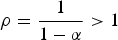 . Consumers maximize (1) subject to the budget constraint
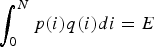 . The price of variety i is p(i) and E is total expenditures on all the varieties of the differentiated good. Then, the demand for variety i is given by:

where 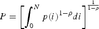 is the aggregate price of the good.
The representative consumer supplies L unit of labor inelastically and has the following utility function:

where Z and Q denote the consumption of homogeneous and differentiated goods respectively. With this Cobb–Douglas preference, β is the share of differentiated good in total output Y, hence E = β Y.
The supply side in a differentiated-good sector is characterized by monopolistically competitive firms producing different varieties. Firms differ in terms of their productivity ϕ.Footnote 6 The only factor of production is labor, hence ϕ refers to labor productivity. A firm learns its productivity, drawn from a known distribution function with a cdf G(ϕ), only after it enters the industry paying a fixed cost, f e. Marginal cost of a firm with productivity ϕ is 1/ϕ. Firms also have to pay a per-period fixed cost of production f d. If a firm with productivity ϕ decides to produce, then the profit-maximizing price is  , which is a constant markup over the marginal cost. Hence, the quantity, revenue and the profit of the firm are, respectively:

The profit function can be written in a compact way as:

where 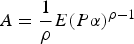 and
 .
In an open economy framework, firms also have an opportunity to serve foreign markets. For expositional simplicity, we consider two symmetric countries.Footnote 7 Firms can exploit foreign markets either by exporting or by directly investing in those countries.
Exporters have to pay fixed export costs f x and also have to bear variable trading costs. Variable trading costs are of the iceberg type, so that τ > 1 units have to be shipped for one unit to arrive at a destination. This extra variable trade cost is reflected in the price in the export market,  . Since the demand is elastic (ρ > 1), revenues in export markets are reduced by τ1−ρ. By the symmetry assumption, price index P and expenditures E are the same for both countries. Therefore, profits from export sales are
 . Profits from exports can be written as:

Firms might also choose to serve foreign markets through FDI. By producing directly in the foreign country, firms can avoid variable trading cost τ. However, the fixed cost of direct investment f i is higher than f x. The symmetry assumption implies  . Therefore,

There is free entry and firms die at an exogenous rate δ. In the steady state, the number of entrants is equal to the number of those that exit; hence the number of firms stays constant. New firms enter as long as expected profit from entry exceeds the cost of entry f e. After paying the fixed cost of entry, a firm observes its productivity level and stays in the market if it makes a non-negative profit. Since the profits are an increasing function of productivity, there will be a productivity cutoff ϕ* such that firms with productivity higher than the cutoff stay while firms that draw lower productivity exit. The cutoff level of productivity is determined by:

Free entry implies that firms continue to enter until the present value of expected profits is equal to the entry cost:

where  is the expected profit of surviving firms.
Firms also export as long as they make a profit from export sales  . Then, the exporting cutoff can be found by:

We can express ϕx in terms of exit cutoff ϕ* by substituting (6) into (5):

Exporters have higher productivity than firms that serve domestic markets only if  .
Firms can avoid variable trading costs by investing directly in foreign countries. However, direct investment requires a higher fixed cost. Firms choose to be involved in FDI instead of exporting if they make a higher profit  . Hence, FDI cutoff is determined by:

We can express FDI cutoff ϕi in terms of entry cutoff ϕ* as:

We have the sorting pattern that the most productive firms are involves in FDI, less productive ones export and even less productive firms operate only in domestic markets if  .
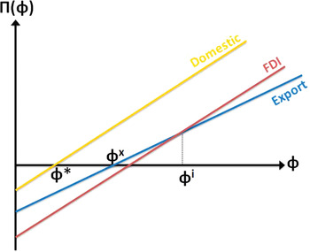
Figure 1 plots equations (2), (3) and (4). This figure illustrates the whole idea clearly: firms with productivity less than Φ* exit; firms with productivity between Φ* and Φx operate in domestic markets only. Firms with productivity between Φx and Φi serve both domestic and foreign markets by exporting. Finally, firms that have productivity higher than Φi serve foreign markets through FDI.
Domestic firms, exporters and multinationals
Notes: Figure displays productivity cutoffs: firms with productivity less than Φ* exit, firms with productivity between Φ* and Φx operate in domestic markets only. Firms with productivity between Φx and Φi serve both domestic and foreign market by exporting. Firms that have productivity higher than Φi serve foreign markets through FDI.

Once ϕx and ϕi are expressed in terms of ϕ*, one can solve for ϕ* using the free entry condition. Equations (5), (6), (7), along with the free entry condition, provide an implicit solution for cutoff values ϕ*, ϕx and ϕi and the demand level.
2.2. Environmental regulations
In this section, we introduce environmental regulations in one country, which bring additional costs to producers in the regulated country. We model this as an additional per-period fixed cost of production f a.
The regulations affect the profits from domestic and export sales, but not the profits from FDI. Due to this extra cost of abatement, the least efficient firms will be driven out of the market, while some firms that export before the regulations will switch to FDI as a way to serve in the foreign market.
First, we express FDI cutoff as a function of export cutoff asFootnote 8:

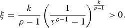
The ratio of exporters to multinationals is 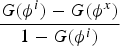 . We use the Pareto distribution with a cumulative distribution function G(ϕ) = 1 − (ϕ)−k.Footnote 9 Thus, the relative share of exporters is
 , and can be written as a function of parameters:

Proposition
After the regulations the ratio of exporters to multinationals decreases.
Proof: 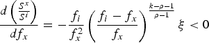 .Footnote 10 Note that after regulations, the fixed cost of exporting becomes f x + f a > f x for any f a > 0. □
Some firms that used to export before regulations find it more profitable to invest directly in the foreign country, rather than exporting the good after producing it in the domestic country (where they face an additional abatement cost).
Regulations also increase the exit cutoff. Since the new fixed cost of domestic production is f d + f a higher, lowest productivity firms leave the market after regulations are established.
This model delivers the results some economists have in mind when they argue that uneven environmental regulations do not help to reduce pollution as firms will find unregulated markets (pollution havens) for their polluting production activities. Moreover, employment and output deteriorate in the regulated markets when some firms exit the market altogether, and others move their production to unregulated pollution havens. However, in the next section, using Chilean microdata, we show that foreign firms emit less than their domestic counterparts and the current model cannot explain this. Multinationals from regulated markets have no incentive to reduce their pollution in unregulated markets. They do not have to pay an extra abatement cost. In fact, this is why some firms move to unregulated markets after regulations are put in place. Yet, we find that even if we control for productivity, foreign firms in Chile are cleaner than domestic firms. Therefore, we introduce a technology upgrading option to firms in the next section. We base our model on the evidence that regulations may in fact improve productivity (Jaffe et al., Reference Jaffe, Peterson, Portney and Stavins1995).
2.3. Regulations and technology upgrading
This section models an environment where firms have two ways to comply with environmental regulations. One is to pay a per-period fixed cost f a and the other is to pay a higher fixed cost f t and adopt cleaner technology. This model builds upon two assumptions:
1. Cleaner technology enables firms to comply with regulations and also improves their productivity. If a firm with productivity ϕ adopts the clean technology, it pays a per-period fixed cost of f t, and its productivity becomes γ ϕ where γ > 1.Footnote 11
2. Once a firm pays f t and upgrades its technology, it can duplicate the same technology in other countries at a lower cost ηf t, η < 1.Footnote 12
We isolate our model from an export decision since it makes the model unnecessarily complicated. Ignoring the export option does not affect our analysis.Footnote 13
In this model, we still have an exit cutoff determined by the following equation:

Firms also exploit the foreign market through FDI if they find it profitable to do so. Hence the FDI cutoff is given by:

We can express FDI cutoff ϕi in terms of ϕ*:

As long as f i > f d, only the most productive firms are involved in FDI.
Before the regulations, firms do not choose to upgrade their technology:

Note that the left-hand side of the inequality is constant while the right-hand side increases in ϕ. Since ϕ has an infinite support (ϕ∈ [1,∞)), there should be a point where this expression holds with equality. Even in the absence of any regulations for some highly productive firms, it is profitable to upgrade. For simplicity we assume, in the rest of the paper, that this technology is not available to firms before the regulations.
Next, we introduce environmental regulations. We assume that the regulated market is a big country (the United States or Germany) while the unregulated economy is a small open economy (Chile).
2.3.1. Regulated economy
When the environmental regulations are introduced, firms in the regulated country need to compare:

The marginal firm that is indifferent to the choice between adopting the clean technology and using old technology and paying an abatement cost is determined by the equality of these two terms:

The marginal firm might be a domestic firm or a multinational but this does not affect our results qualitatively, hence we assume the marginal firm is a multinational.Footnote 14 Therefore, some firms in the regulated market choose to upgrade their technology and these firms also operate in the foreign (unregulated) market.
Under the regulations the exit and FDI cutoffs are determined by:
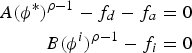
where A and B are the demand levels in the regulated and unregulated economies respectively.
The equation that determines the technology adoption cutoff can also be written as:

Thus, we can express the technology cutoff in terms of exit cutoff as:

The following condition on parameters assures the existence of firms that choose not to upgrade but to pay f a (ϕh > ϕ*):

Multinationals do not face environmental regulations in the foreign country. However, once a firm adopts the clean technology, it can duplicate the technology in another location at a lower cost. Therefore some multinationals find it profitable to upgrade their technology abroad even if they do not have to worry about regulations. The technology cutoff for multinationals is determined by:

and the cutoff point in terms of the FDI cutoff is:

Conditional on ϕh,i > ϕi or 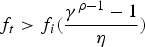 , some multinationals continue to use the old technology abroad even if they adopt the clean technology at home. Finally, the free entry condition for the home country is given by:

2.3.2. Unregulated economy
Firms that operate in the country where there are no environmental regulations (or where regulations are not enforced) do not bear any cost for their emissions. They take the demand level as given and decide whether to stay or exit after observing their productivity draw, and also whether to serve the other country via FDI or not. Exit and FDI cutoffs are given by the following equations:


Note that we ignore the possibility of multinationals in the unregulated country upgrading their technologies. The unregulated country is small compared to the regulated economy; there are not many multinationals going to the large country. Thus we think that we do not lose much by ignoring the small-country multinationals that are productive enough to upgrade the technology abroad. The free entry condition for an unregulated economy is given by:

Equations (8)–(12) and the free entry conditions for the two countries provide implicit solutions for the cutoffs and the demand levels.
3. Empirical analysis
3.1. Data
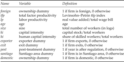
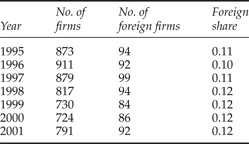
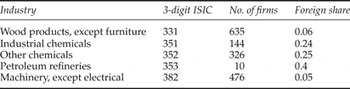
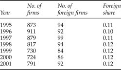
We have a plant-level data set from Chile which covers 1995–2001.Footnote 15 The data include energy expenditures, capital stock, employment, sales, valued added, ownership, geographical variables and industry id among others.Footnote 16 We do not have any data on emissions. Thus, we follow Eskeland and Harrison (Reference Eskeland and Harrison2003) to construct proxies for emission. Using US data, they find that energy intensity is a strong predictor of particulates emissions, and it can provide a good proxy for emissions across industries. They show that it also serves as a reasonable proxy for emissions within certain industries (chemical, petroleum refining, wood and lumber, and nonelectrical machinery). We restrict our analysis to these sectors where energy intensity is a strong predictor of emissions.Footnote 17 We end up with 5,725 observations for seven years (around 800 firms per year).
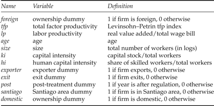
Variable definitions
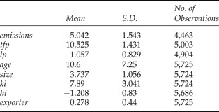
Summary statistics

Note: Variables are in logs except for age and export status. S.D., Standard deviation.
We use total fuels over total sales, and total fuels over total inputs as proxies for emissions. All variables are deflated by appropriate price indices. We get qualitatively the same results with both proxies.
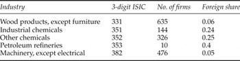
Share of foreign firms: by sector
Share of foreign firms: by year
3.2. Are foreign firms cleaner or dirtier?
Before going into a formal regression analysis we first plot the distributions of certain variables that give a rough picture of the environmental performance of domestic vs. foreign firms.
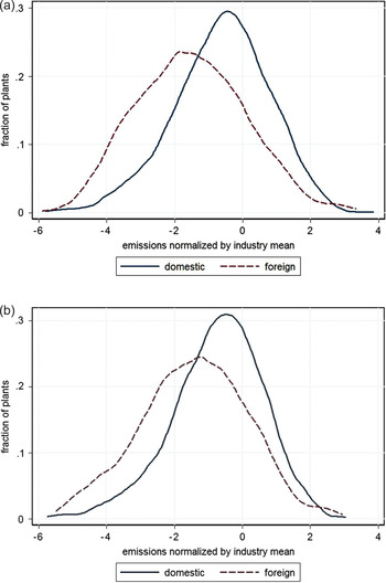
Figure 2 plots the distribution of our emissions proxy for foreign and domestic plants. The first panel shows the distribution of the variable normalized by the overall mean, and the second normalizes it by the industry mean for each year. The distribution of emissions for domestic plants dominates the distribution of foreign plants. This suggests that domestic plants emit, on average, more than foreign firms.Footnote 18
Distribution of emissions
Notes: Figure plots the distribution of the proxy for emissions. Distributions are normalized by overall mean in panel (a) and by industry mean in panel (b). Kolmogorov–Smirnov and t-tests show that distributions for domestic and foreign firms differ significantly, and have different means.

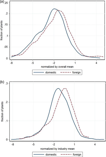
Figure 2 illustrates that foreign plants use less fuel per unit of output, and that they have a lower share of fuels in total input.Footnote 19 Foreign-owned plants also differ from domestic ones in the sources of energy they use. Figure 3 plots the ratio of electricity to fuel. This ratio is, on average, higher for foreign plants. Foreign plants seem to favor the use of electricity over fuels. Electricity is a cleaner source of energy compared to fuels.Footnote 20 Therefore, foreign plants are not only more fuel efficient but also use cleaner sources of energy.
Electricity over fuels
Notes: Figure plots the ratio of electricity to fuel. Foreign plants favor the use of electricity over fuels. Distributions are normalized by overall mean in panel (a) and by industry mean in panel (b). Kolmogorov–Smirnov and t-tests show that distributions for domestic and foreign firms differ significantly, and have different means.

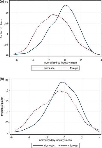
Finally, we consider the most polluting fuels: coal, coke and petroleum. We construct a measure of emissions as a share of these fossil fuels in total input. Figure 4 shows that the distribution of emissions for domestic plants is significantly to the right of the distribution for foreign plants, suggesting that domestic plants use highly polluting fuels more intensively.Footnote 21
Share of dirty fuels in total input
Notes: Figure considers the most polluting fuels: coal, coke and petroleum. The measure of emissions is the share of these fossil fuels in total input. Domestic plants use highly polluting fuels more intensively. Distributions are normalized by overall mean in panel (a) and by industry mean in panel (b). Kolmogorov–Smirnov and t-tests show that distributions for domestic and foreign firms differ significantly, and have different means.

Preliminary data analysis indicates that foreign plants tend to be cleaner than their domestic peers. Now we present a more detailed analysis. We identify the effect of foreign ownership on the emissions of plants in a regression framework, controlling for the explanatory variables used in the previous literature (Eskeland and Harrison, Reference Eskeland and Harrison2003; Cole et al., Reference Cole, Elliott and Shimamoto2005, Reference Cole, Elliott and Strobl2008).
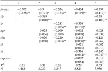
In order to analyze the effect of ownership on emissions, first we perform a regression of emissions on ownership, controlling for industry, year and region.Footnote 22 We control for region to capture the effect of location-specific factors that would affect emissions of firms. The second regression controls for total factor productivity (tfp), size and age.Footnote 23Size is total number of workers (in logs). The third specification includes labor productivity (lp) instead of tfp. Labor productivity is real value added over total wage bill, which is real value added per worker in efficiency units. The last two columns control for capital intensity (ki), human capital intensity (hi) and export status (exporter) in addition to the previous variables. Capital intensity is capital stock per worker, human capital intensity denotes the share of skilled workers in total work force, and export status is a binary variable that indicates whether a firm exports or not. All variables except for age and dummies are in logs. We estimate the following regression:

where E i, s, t denotes the emissions of firm i in industry s at time t, foreign is the ownership dummy that takes a value of 1 if a plant is foreign owned, and X is a vector of control variables that includes tfp, lp, size, age, ki, hi and exporter.Footnote 24
Table 5 shows the results.Footnote 25 The coefficient on the ownership dummy (β1) is negative and significant in all specifications. Controlling for year, three-digit industry and region, foreign firms tend to emit 70 per cent less. β1 is still significant even if we control for other variables, but it is smaller in absolute value when we include productivity. Foreign plants emit 30 per cent less if we control for tfp, age and size. The coefficient for tfp is also negative and significant. This indicates that more productive plants are also cleaner. Not including tfp causes an upward bias on the foreign dummy, since foreign plants are, on average, more productive than domestic plants.
The effect of ownership on emissions

Notes: Robust standard errors in parenthesis, clustered by plant. *significant at 5%; **significant at 1%. All specifications include year, industry and regional dummies.
We use age to capture the fact that foreign plants might be newer and cleaner.Footnote 26 However, the coefficient on age is not significant. Size does not appear significant in the second and the last columns, probably because the effect of size is already captured in tfp. We get similar results when we use labor productivity instead of tfp. The coefficient on foreign dummy is still negative and significant. Foreign plants emit 52 per cent less.Footnote 27 Productivity also has a negative sign. Thus, the more productive a plant is, the less it pollutes.
Export status is not significant in any of the specifications. This suggests that once we control for ownership and productivity, being an exporter is not relevant to emissions. The coefficient on capital intensity is positive but not significant, while human capital intensity has a negative and significant coefficient in both specifications.Footnote 28 Firms that have higher shares of skilled workers tend to emit less. Capital intensity also appears to be associated with high energy use.Footnote 29 We still get negative and significant coefficients on foreign ownership even if we control for the fact that foreign plants are more intensive in both physical and human capital.
3.3. Introducing stricter regulations in the developing economy
Now, we ask what happens if the host country decides to strengthen its environmental regulations as well. Our model implies that, in this case, some domestic firms (the less productive ones) exit the market. Since the multinational firms are the most productive ones, and some of them have already implemented the clean technology, the regulation does not hurt multinational firms as much as domestic ones.
To test this prediction of our model we use the cap and trade regulation in the Santiago metropolitan area. We analyze the exit rate of domestic and foreign firms in a difference in difference in difference regression (DDD).Footnote 30 Because of the serious air quality problems that faced the Santiago metropolitan area, in 1992 the government implemented an emission trade for particulate matter from stationary combustion sources (industrial and commercial boilers, industrial ovens and power plants). The program had two phases. The first, from 1994 to 1999, had a default concentration of 56 mg/m3 of PM10 concentrations. For the second, the concentration was reduced to 50 mg/m3.Footnote 31 We use this strengthening in the regulation to do a DDD experiment and study how firms react to the change in the cap.
We use firms in Santiago as the treatment group and the firms in the rest of the country as the control group. Pre-treatment is the first phase; post-treatment is the second one. Finally, since we conjecture that the outcome for domestic and foreign firms is different, we add a control for ownership. We run the following DDD regression:

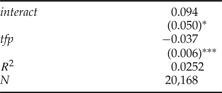
where Exit is 1 if firm i exits and 0 otherwise, and interact is the interaction of three dummies (interact = post i,s,r,t × santiago i,s,r,t × domestic i,s,r,t). The variable post is the dummy variable for observations after the strengthening of the regulation, santiago is the dummy variable for firms in the Santiago metropolitan area and domestic is a dummy for domestic firms. The vector Z includes the dummies post, santiago, domestic and the three pairwise interactions between them. Again, X includes tfp, emission, size, age, ki, hi and exporter and the interaction of tfp and emission. We also include year, region and industry dummies. We use all industries.Footnote 32
We are interested in coefficient β1, which shows the differential effect of the treatment on domestic firms in the Santiago metropolitan area. Table 6 displays the results.Footnote 33 Our coefficient of interest is positive and significant, implying that the exit rate for domestic firms was 9 per cent higher than for foreign firms after the strengthening of the emission cap in the Santiago metropolitan area. This result supports the prediction of our model: as foreign firms are on average cleaner than domestic ones, stiffening regulations hurt domestic firms the most. Some of them cannot afford to comply with regulations and exit the industry.
The effect of strengthened regulations on exit
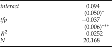
Notes: Robust standard errors in parenthesis, clustered by plant. *significant at 10%; **significant at 5%; ***significant at 1%. All specifications include year, industry and regional dummies.
4. Concluding remarks
In this paper, we study the environmental effects of foreign firms in host countries. We introduce a theoretical model where we add environmental regulations into a standard trade model with heterogeneous firms and monopolistic competition. Firms have the option to pay a fixed cost and comply with the regulation or pay a higher fixed cost and adopt a more productive, cleaner technology. The more productive firms (those firms involved in FDI) are the ones that adopt the more productive technology. Moreover, it is optimal for some multinationals to take the cleaner, more productive technology abroad where they face no regulations.
We use plant-level data from Chile and find that foreign firms are in fact cleaner than domestic ones, even controlling for other factors such as productivity, size, age, human capital and capital intensity and exporter status. We also find that the exit rate of domestic firms increases more after a strengthening in regulations in the Santiago metropolitan area. This is consistent with the model because multinational firms are the most productive ones, and some of them already have a cleaner technology. Thus, the regulation does not hurt multinational firms as much as domestic ones.
One limitation of our paper is that, in the model, firms involved in FDI do so only to serve the foreign markets. Hence, the model only captures horizontal FDI. A similar analysis with a model of vertical FDI might deliver different results. We therefore avoid claiming that the PHH is totally irrelevant. What we argue is that empirical evidence shows that environmental claims against multinationals are tenuous. Our model also introduces mechanisms that we cannot fully examine. A data set with information on the multinationals from a developed country, and their affiliates in developing countries, would allow us to test whether the mechanisms described in our model are actually in force.
If data are available, one can, for example, test whether the multinationals are cleaner than domestic firms in developed countries as well, or whether the average emission of foreign firms in a developing country is similar to the average emission of the same firms in their home country. Therefore, we believe, this paper will stimulate more research on the topic.
Appendix
The data are from an annual survey of Chilean manufacturing plants (ENIA). The data set includes plants that have more than 10 employees and covers the years from 1979–2001. We focus on 1995–2001 since ownership data before 1995 are not as consistent. The survey provides information on the number of employees, wage bill (for blue-collar and white-collar workers separately), value of production, value of exports, value of energy expenses (fuel and electricity) and raw materials, and total sales, among others.
Capital stock
In our data set, plants begin to report capital stock and/or investment in 1992. Since we have a lot of missing values, we manually reconstruct capital stock. We take the data from 1992 for vehicles, machines and buildings. If a firm does not report capital stock for that year, we impute it. We run three regressions for vehicles, machines and buildings using workers and total sales as explanatory variables. We construct the 1992 capital stock for the missing values as the mean of predicted values for the same three-digit industry. If the following years are missing, we apply the perpetual inventory method given by the following formula using the depreciation rate (δ) of 20 per cent for vehicles, 10 per cent for machines and 5 per cent for buildings:

We also construct another measure of capital stock. We use the same procedure but instead of treating vehicles, machines and buildings separately, we sum them and follow the same methodology, assuming an overall depreciation rate of 10 per cent. Our results are not sensitive to choice of measure of capital stock, but we stick to the first one since we think that measure is more accurate.
Tfp index
We follow the Levinsohn–Petrin method to construct a tfp measure (Levinsohn and Petrin, Reference Levinsohn and Petrin2003). Basically, tfp is calculated as residuals from a production function of the following form:

where small letters indicate logs of variables. Olley and Pakes (Reference Olley and Pakes1996) show that OLS on this equation is inconsistent because of endogeneity and selection problems. They suggest an alternative calculation, using panel data for firms with investment. Levinsohn and Petrin (Reference Levinsohn and Petrin2003) built their method on the work of Olley and Pakes (Reference Olley and Pakes1996), taking the possibility of zero values and missing investment into the account.
We use stata command ‘levpet’, which estimates production functions using intermediate inputs to control for unobserved productivity shock based on the methodology described in Levinsohn and Petrin (Reference Levinsohn and Petrin2003). We estimate value-added-based production function for each two-digit industry by using raw materials and electricity as proxies for investment. tfp is calculated as:

where Q i is real value-added, L iw is white-collar and L ib is blue-collar workers.
Foreign dummy
Foreign is a dummy that takes the value of 1 if the firm is foreign. Ownership data include the following categories: domestic, foreign, mixed and state. We consider two different criteria in constructing the dummy. In the first case we assume all mixed plants are foreign, and in the second case we assume plants that have at least 10 per cent foreign share are foreign. Our results do not vary a lot, so we choose to remain with the first case. With regard to state-owned plants we have two options. Either we exclude these plants from the analysis or we assume that they are domestic. Our results are not sensitive to this choice since there are only a few of them. We opt for the second option.
Price indexes
We have a three-digit industry price deflator and input price deflator. The base year is 1996 for both indices. We use the former to calculate real sales and real value added. We deflate electricity, fuels and raw materials by using the latter.
 .