


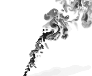



1. Introduction
Turbulent buoyant plumes have long been studied due to their ubiquity in nature and in industry, and their importance in fields such as disaster management and industrial pollution. Examples are volcanic eruptions, pollutant dispersion via chimneys, fires, ocean outfalls and jet engines (Woods Reference Woods2010; Mahesh Reference Mahesh2013). A significant number of parameters play a role in the evolution of a buoyant plume. These include the source velocity, release angle, density and the state of the atmosphere the plume ascends through via the velocity profile  $\boldsymbol {U}(z)$ and the stratification, characterised by the (square) buoyancy frequency
 $N^2(z)$. Volcanic applications feature another level of complexity due to the initial ash volume fraction and its size distribution, ash reactivity and compressibility effects including shock waves due to supersonic conditions at the source.
Buoyant plumes are typically modelled via integral models. The now-classical plume equations were presented in Morton, Taylor & Turner (Reference Morton, Taylor and Turner1956), and comprise a set of three coupled ordinary differential equations for the volume flux  $Q$, (streamwise) momentum flux
 $M$ and buoyancy flux
 $F$, respectively. This theory was formulated in the absence of a crossflow such that the plume only evolves in the vertical coordinate
 $z$. One of the cornerstones of the theory is the entrainment assumption, which links the entrainment of fluid into the plume to the characteristic velocity inside the plume. Morton et al. (Reference Morton, Taylor and Turner1956) assumed that the entrainment coefficient
 $\alpha$ was constant, although different values of
 $\alpha$ are typically used for jets and plumes. Recent work by van Reeuwijk & Craske (Reference van Reeuwijk and Craske2015) has clarified the relation between the Morton et al. (Reference Morton, Taylor and Turner1956) model and the Priestley & Ball (Reference Priestley and Ball1955) model, who used a closure involving the production of turbulent kinetic energy. Analysis of experimental and numerical data by van Reeuwijk & Craske (Reference van Reeuwijk and Craske2015) indicated that for jets and plumes the more suitable model is that of Priestley & Ball. In fully self-similar conditions, and with the buoyancy and velocity profiles having an equal width (List Reference List1982), it follows directly that
 $\alpha _{plume} \approx (5/3) \alpha _{jet}$ (van Reeuwijk et al. Reference van Reeuwijk, Salizzoni, Hunt and Craske2016).
Integral plume models were extended to crossflows by, for example, Briggs (Reference Briggs1982) and Weil (Reference Weil1988) and references therein: for strongly bent-over plumes they showed that analytical expressions could be derived for the level of neutral buoyancy and the maximum rise height of the plume. This involved adding an ordinary differential equation for the horizontal momentum excess flux  $M_x$. The presence of a crossflow fundamentally alters the entrainment properties of a plume: it typically causes the flow to bend over and organise itself into a double-roll structure with two turbulent counter-rotating vortices (Fischer et al. Reference Fischer, Koh, Imberger and Brooks1979; Weil Reference Weil1988; Huq & Dhanak Reference Huq and Dhanak1996). For jets in a crossflow, Mahesh (Reference Mahesh2013) summarises the research of the double-roll structure and describes the horseshoe and wake vortices which form upstream of the jet's leading edge as a result of adverse pressure gradients.
In parallel with the effort to develop a suitable integral plume model, there is a large body of literature documenting experimental and numerical surveys of plumes in a crossflow (e.g. Cintolesi, Petronio & Armenio Reference Cintolesi, Petronio and Armenio2019). One of the earliest experimental studies (Fan Reference Fan1967) investigates two categories of plumes: inclined plumes discharged into a stratified but quiescent environment, and plumes discharged into a homogeneous, uniform crossflow. Subsequent studies have been carried out for a wide range of initial and boundary conditions, resulting in a large catalogue of experimental work. For example, Gaskin (Reference Gaskin1995) compares a plume in a quiescent environment to a plume with a uniform crossflow, and Huq & Stewart (Reference Huq and Stewart1996) assess the effects of atmospheric turbulence on plume development. With the increasingly widespread availability of high-powered computing, numerical studies and particularly large-eddy simulations (LES) have become an additional powerful tool for investigating plume dynamics. Yuan, Street & Ferziger (Reference Yuan, Street and Ferziger1999) were early innovators in this regard, simulating jets in a crossflow (without buoyancy) by utilising a dynamic Smagorinsky model for the subgrid scales. They used their LES to analyse the counter-rotating vortex structure, concluding that it was the result of the hanging vortices which appear in the region close to the source of the jet. More recently, De Wit, Van Rhee & Keetels (Reference De Wit, Van Rhee and Keetels2014) examined a real-world application of LES to overflow dredging plumes resulting from a moving dredger. They discovered that the average horizontal velocity of the plume exceeds the speed of the crossflow. We discuss this intriguing phenomenon in §§ 6 and 7. Another pertinent numerical study is that of Devenish et al. (Reference Devenish, Rooney, Webster and Thomson2010) presenting LES of purely buoyant plumes released into stratified and uniform environments. They compared the results of their LES with plume integral models and proposed a modified entrainment assumption in which the contributions from the horizontal and vertical velocity components are not equally weighted.
There are various entrainment assumptions (see § 5), and all involve some mix of the plume velocity and the crossflow speed. Most models assume that the pressure is hydrostatic within the plume at least when averaged over the plume cross-section, and that the effects of pressure can be represented by an added-mass coefficient. Most models also neglect the Leibniz term: the increase in (for example) integral volume flux as a result of the spreading of the plume into a non-quiescent atmosphere. Schatzmann (Reference Schatzmann1978), on the other hand, fully integrated the governing equations and was the first to describe an integral plume model incorporating the Leibniz term. He argued that this term should not be counted towards entrainment, since it requires a fundamentally different interpretation of the entrainment coefficient. In addition, he noted the need for a pressure term, although at the time not enough was known to fully model it. Limitations of his analysis are the assumption of axisymmetry and the assumption that the turbulence terms are negligible. We avoid these assumptions in our analysis by integrating the Reynolds-averaged equations directly, allowing us to assess all terms in the integral budgets and to determine which are physically relevant and which can be ignored.
One pertinent example of an application in which integral models play a key role is in the determination of the mass flux of a volcanic eruption. It is not possible to measure this quantity directly, so the mass flux is often inferred from the rise height of the plume, which is where the plume has the same density as the surrounding atmosphere and starts spreading laterally like a gravity current. Turbulent entrainment thus plays a key role in the rise height, since this is the sole mechanism by which the plume dilutes. Appropriately incorporating the influence of crossflow in these estimates is key for appropriate estimation of the source mass flux (Devenish Reference Devenish2013; Woodhouse et al. Reference Woodhouse, Hogg, Phillips and Sparks2013; Costa et al. Reference Costa2016; Rossi, Bonadonna & Degruyter Reference Rossi, Bonadonna and Degruyter2019).
The aim of this paper is to examine the assumptions underlying integral models of plumes in a crossflow, including entrainment, by means of direct numerical simulation (DNS). In order to manage the complexity of the problem, we restrict ourselves to a neutral atmosphere ( $N=0$) with a uniform crossflow speed
 $U$ and a momentumless source (i.e. an infinitely lazy plume). The only parameter that is varied is the crossflow speed. We focus our attention on the behaviour exhibited by plumes with a strong crossflow, and on developing a model for the entrainment and pressure drop over the plume.
2. Theory
2.1. Integral equations
In this section, equations for the integral volume, momentum and buoyancy fluxes are derived. The derivation is consistent with that of Weil (Reference Weil1988) and Schatzmann (Reference Schatzmann1978), but is performed here without any simplifications, such as the assumption of axisymmetry (Schatzmann Reference Schatzmann1978) or neglecting turbulence and pressure terms. A schematic detailing the nomenclature used here is given in figure 1. Cartesian coordinates  $(x, y, z)$ are used which represent the streamwise, transverse and vertical directions, respectively. The crossflow speed in the
 $x$ direction is denoted
 $U$ and is uniform in
 $z$. It is convenient to also introduce a plume-following coordinate system
 $(s,y,\eta )$, where
 $s$ is the distance from the source along the plume centreline,
 $y$ is the transverse direction (which remains unchanged) and
 $\eta$ is the coordinate perpendicular to
 $s$ in the
 $(x, z)$ plane. The plume centreline makes an angle
 $\varphi$ with the
 $x$ axis. The plume source is positioned at (0, 0, 0) and the release is momentumless with a constant integral buoyancy flux
 $F_0 = r_0^2 \phi _b$, where
 $r_0$ is the source radius and
 $\phi _b$ is the (diffusive) buoyancy flux. This infinitely lazy plume condition is chosen so as not to introduce a further parameter, namely the source momentum flux, and to manage the complexity of the problem.
A schematic of the plume with the Cartesian  $(x,z)$ coordinate system and the curvilinear
 $(s, \eta )$ coordinate system. The
 $y$ direction is perpendicular to this plane. Values for
 $L_x$,
 $L_z$ and
 $L_n$ for the five simulations can be found in table 1.

The incompressible Navier–Stokes equations with the Boussinesq approximation are
 \begin{gather} \boldsymbol{\nabla}\boldsymbol{\cdot} \boldsymbol{u} =0, \end{gather}
 \begin{gather}\frac{\partial\boldsymbol{u}}{\partial t} + \boldsymbol{u}\boldsymbol{\cdot}\boldsymbol{\nabla}\boldsymbol{u} ={-}\boldsymbol{\nabla} p + \nu \nabla^2 \boldsymbol{u} + b \boldsymbol{\hat{k}}, \end{gather}
 \begin{gather}\frac{\partial b}{\partial t} + \boldsymbol{u}\boldsymbol{\cdot}\boldsymbol{\nabla} b = \kappa \nabla^2 b, \end{gather}
where  $\boldsymbol {u} = (u,v,w)$ is the velocity of the fluid,
 $b=g (\rho _0 - \rho ) / \rho _0$ is the buoyancy and
 $p=\tilde p/\rho _0 + gz$ is the kinematic pressure perturbation, where
 $g$ is the gravitational acceleration,
 $\rho _0$ is a constant reference density and
 $\tilde p$ is the standard pressure. The kinematic viscosity and scalar diffusivity are denoted by
 $\nu$ and
 $\kappa$, respectively. Assuming high-Reynolds-number and high-Péclet-number flow, applying Reynolds averaging to (2.1) and making use of the fact that the flow is statistically steady results in
 \begin{gather} \boldsymbol{\nabla} \boldsymbol{\cdot} \bar{\boldsymbol{u}} = 0, \end{gather}
 \begin{gather}\boldsymbol{\nabla} \boldsymbol{\cdot} (\bar{\boldsymbol{u}}\overline{u_i} +\overline{\boldsymbol{u}'u_i'}) ={-}\frac{\partial\bar{p}}{\partial x_i} + \bar{b} \delta_{i3}, \end{gather}
 \begin{gather}\boldsymbol{\nabla} \boldsymbol{\cdot} (\bar{\boldsymbol{u}}\bar{b} +\overline{\boldsymbol{u}'b'}) = 0, \end{gather}
where the overbars denote time averaging and fluctuating quantities are defined as  $\phi '=\phi -\bar {\phi }$ for any variable
 $\phi$.
Using that  $\overline {\boldsymbol {u}} \bar {\phi } + \overline {\boldsymbol {u}'\phi '}=\overline {\boldsymbol {u} \phi }$, the equations above are all of the form (e.g. Weil Reference Weil1988)
 \begin{equation} \boldsymbol{\nabla} \boldsymbol{\cdot} \left(\overline{\boldsymbol{u}\phi}\right) = G, \end{equation}
which can be integrated over the plume cross-section  $A$, whose domain is denoted
 $\varOmega$, to obtain (van Reeuwijk, Vassilicos & Craske Reference van Reeuwijk, Vassilicos and Craske2021) (see Appendix A)
 \begin{equation} \frac{\text{d}}{\text{d} s} \displaystyle\iint_\varOmega \bar{u}_s \bar{\phi} + \overline{{u}'_s\phi'} \,\text{d} A = \displaystyle\iint_\varOmega G\,\text{d} A + {\rm \pi} E[\phi] + {\rm \pi} \mathcal{L}[\phi], \end{equation}
where  $\bar {u}_s=\bar {u} \cos \varphi + \bar {w} \sin \varphi$ is the mean velocity in the
 $s$ direction and
 $\varOmega (s)$ represents the domain occupied by the plume. See § 3.2 for a description of how
 $\varOmega$ is determined practically. In deriving the equation above it was assumed that the curvature of the plume trajectory
 $\text {d} \varphi / \text {d} s \ll 1$ (see Appendix A for more details). The boundary terms
 $E[\phi ]$ and
 $\mathcal {L}[\phi ]$ are line integrals of the form
 \begin{equation} E[\phi] = \frac{1}{{\rm \pi}}\oint_{\partial \varOmega} \overline{\boldsymbol{u}_\perp \phi} \boldsymbol{\cdot} \boldsymbol{n}\, \text{d} \ell, \quad \mathcal{L}[\phi] = \frac{1}{{\rm \pi}}\oint_{\partial \varOmega} \overline{u_s \phi} \frac{N_s}{| \boldsymbol{N}_\perp|}\, \text{d} \ell, \end{equation}
where  $\partial \varOmega$ denotes the plume boundary,
 $\boldsymbol {N} = (N_s, N_y, N_\eta )^\textrm {T}$ denotes the three-dimensional inward-pointing normal along
 $\partial \varOmega$,
 $\boldsymbol {N}_\perp = (N_y, N_\eta )^\textrm {T}$ and
 $\boldsymbol {u}_\perp = (u_y, u_\eta )^\textrm {T}$ are the vector components in the
 $(y, \eta )$ plane and
 $\boldsymbol {n} = \boldsymbol {N}_\perp / |\boldsymbol {N}_\perp |$ is the inward-pointing two-dimensional normal in the
 $(y, \eta )$ plane. As the plume boundary will be detected via the average buoyancy field
 $\bar {b}$ (see § 4),
 $\boldsymbol {N}$ is defined as
 $\boldsymbol {N} = \boldsymbol {\nabla } \bar {b} / | \boldsymbol {\nabla } \bar {b}|$ (see also van Reeuwijk et al. Reference van Reeuwijk, Vassilicos and Craske2021). The factor
 $1/{\rm \pi}$ in the definition of
 $\mathcal {L}[\phi ]$ and
 $E[\phi ]$ is introduced for consistency with the convention in plume theory of dividing the integral quantities through by
 ${\rm \pi}$ (see (2.7)).
The terms  $E[\phi ]$ and
 $\mathcal {L}[\phi ]$ represent distinct physical processes by which the quantity
 $\phi$ enters the plume. The term
 $E[\phi ]$ represents the advection of
 $\phi$ into the plume; the term
 $\mathcal {L}[\phi ]$ represents incorporation of the quantity
 $\phi$ via expansion of the plume into a non-quiescent atmosphere – if the plume surface area
 $A$ over which the governing equations are integrated changes as a function of
 $s$, and the value of
 $\phi$ at the boundary of the plume is non-zero, then the surface integral will be increased by a quantity equal to
 $[{\overline {u_s\phi }}]_b \,\text {d} A/\text {d} s$, where
 ${[\overline {u_s\phi }]}_b$ is the average value of
 $\overline {u_s\phi }$ at the boundary.
Integrating the Navier–Stokes equations over the plume cross-section and applying (2.4) with  $\phi = 1, u-U, w$ and
 $b$, respectively, results in
 \begin{gather} \frac{\text{d} Q}{\text{d} s} = E[1] + \mathcal{L}[1]= E + \mathcal{L}, \end{gather}
 \begin{gather}\frac{\text{d} M_x}{\text{d} s} + \frac{\text{d} M'_x}{\text{d} s} ={-}P_x + E[u-U] + \mathcal{L}[u-U], \end{gather}
 \begin{gather}\frac{\text{d} M_z}{\text{d} s} + \frac{\text{d} M'_z}{\text{d} s} ={-}P_z + B + E[w] + \mathcal{L}[w], \end{gather}
 \begin{gather}\frac{\text{d} F}{\text{d} s} + \frac{\text{d} F'}{\text{d} s} = E[b] + \mathcal{L}[b], \end{gather}
where the integral volume flux  $Q$, the horizontal momentum excess flux
 $M_x$, the vertical momentum flux
 $M_z$, the buoyancy flux
 $F$ and the integral horizontal and vertical pressures
 $P_x$ and
 $P_z$ are defined as
 \begin{equation} \left. \begin{array}{ll@{}} Q = \dfrac{1}{{\rm \pi}} \displaystyle\iint_\varOmega \bar{u}_s \,\text{d} A, & F = \dfrac{1}{{\rm \pi}} \displaystyle\iint_\varOmega \bar{u}_s \bar{b} \,\text{d} A,\\M_x = \dfrac{1}{{\rm \pi}} \displaystyle\iint_\varOmega \bar{u}_s (\bar{u}-U) \,\text{d} A, & P_x = \dfrac{1}{{\rm \pi}} \displaystyle\iint_\varOmega \dfrac{\partial \bar{p}}{\partial x} \,\text{d} A,\\M_z = \dfrac{1}{{\rm \pi}} \displaystyle\iint_\varOmega \bar{u}_s \bar{w} \text{d} A, & P_z = \dfrac{1}{{\rm \pi}} \displaystyle\iint_\varOmega \dfrac{\partial \bar{p}}{\partial z} \,\text{d} A,\\M'_x = \dfrac{1}{{\rm \pi}} \displaystyle\iint_\varOmega \overline{u'_s u'} \,\text{d} A, & F' =\dfrac{1}{{\rm \pi}} \displaystyle\iint_\varOmega \overline{u'_sb'} \,\text{d} A,\\M'_z = \dfrac{1}{{\rm \pi}} \displaystyle\iint_\varOmega \overline{u'_s w'} \text{d} A, & B = \dfrac{1}{{\rm \pi}} \displaystyle\iint_\varOmega \bar{b} \,\text{d} A. \end{array} \right\} \end{equation}
The scalar  $\bar {u}-U$ is chosen for the
 $x$-momentum equation so as to be consistent with the work of Weil (Reference Weil1988) in the definition of
 $M_x$. The integral therefore represents the momentum flux in the
 $x$ direction in excess of the
 $x$-momentum flux of the ambient atmosphere. A consequence of this choice of variable is that the Leibniz and entrainment terms for the
 $x$-momentum equation are significantly reduced, due to the fact that to first order
 $u \approx U$ at the boundary of the plume.
2.2. Plume models
In conventional plume theory  $\bar {u} - U$,
 $\bar {w}$ and
 $\bar {b}$ are assumed to vanish at the plume boundary. In addition
 $\mathcal {L}[1]$ is assumed to be small. It thus follows that all entrainment and Leibniz terms are negligible except for
 $E \equiv E[1]$. Furthermore, it is commonly assumed that the pressure at the plume boundary is equal to the ambient pressure, which implies that
 $P_x$ and
 $P_z$ are zero (although vertical pressure gradients are taken into account implicitly via an added-mass coefficient). The buoyancy integral
 $B = {\rm \pi} ^{-1} \int \bar {b} \text {d} A$ is generally modelled as
 $B=F/U_s$ (Weil Reference Weil1988), where
 $U_s$ is the characteristic velocity of the plume, defined as
 \begin{equation} U_s = (U + u_m) \cos \varphi + w_m \sin \varphi. \end{equation}
Here,  $u_m$ is is the characteristic horizontal plume velocity relative to the crossflow (horizontal velocity excess),
 $w_m$ is the characteristic vertical velocity and
 $\varphi$ is the angle of the plume. These characteristic quantities are linked to the integral quantities by
 \begin{equation} Q = r_m^2 U_s, \quad M_x = r_m^2 U_s u_m, \quad M_z = r_m^2 U_s w_m, \quad F = r_m^2 U_s b_m. \end{equation}
Here,  $b_m$ is the characteristic buoyancy or reduced gravity and
 $r_m$ is the characteristic plume radius. Equation (2.9a–d) implicitly provides the definition of
 $u_m$,
 $w_m$ and
 $b_m$ as
 $M_x/Q$,
 $M_z/Q$ and
 $F/Q$, respectively. The characteristic radius
 $r_m$ is defined as
 $r_m=(Q/U_s)^{1/2}$ (i.e. using the definition of
 $Q$; (2.9a)), which encapsulates both the pure plume definition
 $r_m = Q/M_z^{1/2}$ for
 $U\ll w_m$,
 $u_m \ll w_m$, and the bent-over solution
 $r_m = (Q/U)^{1/2}$ for
 $U\gg u_m, U \gg w_m$.
The entrainment term  $E$ is typically parameterised as (Weil Reference Weil1988; Devenish et al. Reference Devenish, Rooney, Webster and Thomson2010)
 \begin{equation} E = 2 \gamma r_m w_m, \end{equation}
where  $\gamma$ is the entrainment coefficient and
 $r_m$ and
 $w_m$ are a characteristic radius and vertical velocity, respectively. Invoking the assumptions stated at the start of this section (
 $\mathcal {L} \ll 1$ and
 $E \equiv E[1]$), neglecting turbulent fluxes and substituting (2.10) into the integral equations (2.6a–d) result in
 \begin{equation} \frac{\text{d} Q}{\text{d} s} = 2 \gamma \frac{M_z}{r_m U_s}, \quad \frac{\text{d} M_x}{\text{d} s} = 0, \quad (1+k)\frac{\text{d} M_z}{\text{d} s} = \frac{F}{U_s}, \quad \frac{\text{d} F}{\text{d} s} = 0. \end{equation}
Here  $k$ is the added-mass constant which takes into account the effects of an adverse pressure gradient on the vertical motion (e.g. Weil Reference Weil1988), which compensates for the fact that no explicit integral pressure terms are present. It is introduced by analogy with the motion of a solid body and is equivalent to using a drag term (see Briggs Reference Briggs1982; Schatzmann Reference Schatzmann1978; Davidson Reference Davidson1989). Kinematic relations for the plume trajectory are required to evolve the plume in space:
 \begin{equation} \frac{\text{d} x}{\text{d} s} = \cos\varphi, \quad \frac{\text{d} z}{\text{d} s} = \sin\varphi. \end{equation}
To close the set of equations, the plume angle  $\varphi$ is conventionally assumed to be the angle of the local streamlines
 $\varphi _u$, defined via
 \begin{equation} \tan \varphi_u = \frac{w_m}{U+u_m}. \end{equation}
Under the assumption that  $\varphi = \varphi _u$,
 $U_s$ represents the velocity magnitude
 $\sqrt {(U\!+\!u_m)^2 \!+\! w_m^2}$, which can then be equivalently expressed in terms of the integral quantities as
 $Q^{-1} \sqrt {(Q U+M_x)^2 + M_z^2}$. Here, we make an explicit difference between
 $\varphi$ and
 $\varphi _u$ since it will turn out that these quantities are not identical for the flow cases under consideration (see § 4). When
 $\varphi \ne \varphi _u$, there is a component of velocity in the
 $\eta$ direction:
 \begin{equation} U_\eta ={-}(U + u_m) \sin \varphi + w_m \cos \varphi. \end{equation}
2.3. Bent-over plumes
In this section we briefly provide an overview of analytical results for bent-over plumes in a neutral stratification and a uniform crossflow. Bent-over plumes are defined to have their centreline inclined at a very small angle to the horizontal (in which case the equations are formally equal to those for a line thermal; Briggs Reference Briggs1984; Lee & Chu Reference Lee and Chu2003). This implies that  $w_m \ll U$,
 $u_m \ll U$ and
 $\text {d} s \approx \text {d} x$. Assuming that in this case the entrainment rate is a constant,
 $\gamma = \beta '$, the following relations can be derived (e.g. Weil Reference Weil1988). Integrating the volume flux equation (2.11a) yields
 \begin{equation} r_m = \beta' z_c + r_0, \end{equation}
where  $r_0$ is the source radius. Integrating the vertical momentum flux equation (2.11c) twice and making use of (2.12a,b), (2.13) and (2.15), assuming
 $\varphi =\varphi _u$, results in
 \begin{equation} \frac{z_c}{\ell_b} = \left(\frac{3}{2\beta^2} \right)^{1/3} \left( \frac{x - x_v}{\ell_b} \right)^{2/3} \end{equation}
for  $r_0 \ll \beta ' z_c$, where
 $\ell _b = F/U^3$ is the buoyancy length scale and
 $x_v$ is a virtual origin correction, which is a constant subtracted from the
 $x$ coordinate of the plume trajectory that compensates for any near-field effects. It is necessary because the region close to the source (where
 $r_0 \ll \beta ' z_c$ no longer holds) is not expected to obey the two-thirds law. The value of
 $\beta$ is not equal to
 $\beta '$, because of added-mass effects (Lee & Chu Reference Lee and Chu2003), and the two can be related as
 $\beta = \beta '\sqrt {1+k}$ (Weil Reference Weil1988, p. 164; see also § 8), where
 $k$ is the same added-mass coefficient as in (2.11a–d). Experiments indicate that
 $0.3 \lesssim k \lesssim 1.3$ (e.g. Briggs Reference Briggs1982; Weil Reference Weil1988; Contini et al. Reference Contini, Donateo, Cesari and Robins2011) and
 $0.45 \lesssim \beta ' \lesssim 0.75$ (e.g. Hewett, Fay & Hoult Reference Hewett, Fay and Hoult1971; Hoult & Weil Reference Hoult and Weil1972; Briggs Reference Briggs1984; Weil Reference Weil1988; Huq & Stewart Reference Huq and Stewart1996). Although
 $\beta '$ is a constant coefficient, it may vary between simulations or experiments dependent on factors such as the strength of the crossflow and the initial buoyancy flux
 $F_0$ (Briggs Reference Briggs1984).
Several entrainment models are in use for plumes in a crossflow (Costa et al. Reference Costa2016). The classical model for a bent-over plume (e.g. Briggs Reference Briggs1984; Weil Reference Weil1988) assumes  $\gamma = \beta '$. An entrainment model which is also valid for weak-crossflow plumes is given by (Devenish et al. Reference Devenish, Rooney, Webster and Thomson2010, DRWT)
 \begin{equation} \gamma = \frac{\sqrt[n]{(\alpha w_m)^n + (\beta' U )^n}}{U_s}. \end{equation}
The DRWT model uses two parameters,  $\alpha$ and
 $\beta '$, to account for entrainment due to vertical and horizontal motion, respectively, and assumes that the added-mass coefficient
 $k=0$. Here,
 $\beta '$ refers to the same bent-over entrainment coefficient as the one that is used in (2.15). A further parameter
 $n$ determines the function used to combine the entrainment resulting from the vertical and horizontal momentum into a single entrainment quantity. In their paper, Devenish et al. (Reference Devenish, Rooney, Webster and Thomson2010) test the values
 $n = \{1, 1.5, 2\}$ and conclude that
 $n=1.5$ provides the best match between the model and their LES data.
3. Numerical modelling
3.1. Simulation details
The simulations concern the evolution of a plume in an unstratified environment with a uniform crossflow speed  $U$. A constant integral buoyancy flux
 $F_0$ is imposed on a circular area source of diameter
 $2 r_0$, which is positioned at
 $x=0$. The source has no initial velocity, which implies the plume is infinitely lazy at the source (Hunt & Kaye Reference Hunt and Kaye2005). The buoyancy flux is therefore imposed as a diffusive flux using a Neumann boundary condition, which will be transported through a very thin thermal boundary layer before it becomes convectively unstable and starts rising as a conventional plume.
The relevant non-dimensional parameters for buoyant plumes in a crossflow can be formed from the exit velocity  $w_0=M_{0}^{1/2}/r_0$, the buoyancy velocity scale
 $U_b=(F_0 / r_0)^{1/3}$, the crossflow speed
 $U$, and for completeness the viscous and thermal velocity scales
 $\nu / r_0$ and
 $\kappa / r_0$, respectively. All quantities with subscript zero represent their respective quantities at the source (e.g.
 $M_{0}$ represents
 $M$ evaluated at the source). From these five velocity scales, four dimensionless quantities can be constructed:
 \begin{equation} R_0=\frac{w_0}{U}, \quad Ri_0 = \frac{F_0}{r_0 w_{0}^3} = \frac{b_{0} r_{0}}{w_{0}^2}, \quad Re_0 = \frac{2F_0^{1/3}r_0^{2/3}}{\nu}, \quad Pr = \frac{\nu}{\kappa}, \end{equation}
where  $R_0$ is the jet-to-crossflow speed ratio,
 $Ri_0$ is the source Richardson number,
 $Re_0$ is the source Reynolds number and
 $Pr$ is the Prandtl number. Note that the Froude number, which is also commonly used, is the square root of the reciprocal of
 $Ri_0$. These dimensionless groups are not ideal for the current simulation set-up since
 $w_0=0$ which implies that
 $w_0/U=0$ and
 $Ri_0 = \infty$. In this study, we thus use the crossflow Richardson number
 $Ri_U$, defined as
 \begin{equation} Ri_U = Ri_0 R_0^3 = \frac{F_0}{U^3 r_0} = \frac{U_b^3}{U^3}, \end{equation}
which is the cube of the ratio of the buoyancy velocity scale  $U_b$ to the crossflow speed
 $U$. Equivalently, using the buoyancy length scale
 $\ell _b=F_0/U^3$,
 $Ri_U$ can be interpreted as a ratio of length scales,
 $Ri_U = \ell _b / r_0$.
Five simulations S1–S5 have been performed at different values of  $Ri_U$, details of which are presented in table 1. Simulation S1 reproduces a case characterised by a weak crossflow, with
 $Ri_U=8$, which corresponds to a flow in which the crossflow speed
 $U$ is equal to half the buoyancy velocity scale
 $U_b$. Simulation S2, with
 $Ri_U=2.4$, also represents a weak crossflow. Simulations S4 and S5, with
 $Ri_U=0.5$ and
 $Ri_U=0.3$, respectively, correspond to strong crossflow cases for which
 $U> U_b$. Simulation S3 has
 $Ri_U=1$, which implies that
 $U = U_b$. All simulations use an identical source Reynolds number
 $Re_0 = 1000$ and Prandtl number
 $Pr=1$. This value is chosen because it is the highest value at which the simulations may currently be conducted, due to computational cost. This value of
 $Re_0$ does ensure that the flow is fully turbulent.
Simulation details. The source Reynolds number  $Re_0=1000$ and Prandtl number
 $Pr=1$ for all simulations.

Due to the fact that the strength of the crossflow affects the evolution of the plume, the domain sizes were chosen large enough such that each plume can evolve inside the domain without interacting with its boundaries, but tight enough not to waste computational resources on flow regions where only ambient flow is present. The domain dimensions are given in table 1. Note that the  $x$ coordinate ranges from
 $x/r_0 = -5$ to
 $x/r_0 = L_x/r_0-5$. For all simulations, the percentage of the domain occupied by the plume in the
 $(y, z)$ plane is less than
 $9\,\%$. This is sufficient to ensure that the interactions with the boundaries are negligible. For a row of plumes in a quiescent environment, the mean plume boundaries plotted by Rooney (Reference Rooney2015) show that a plume which spans
 ${\sim }25\,\%$ of the domain is not significantly affected by the competing entrainment of the other plumes. The grid resolution was chosen such that
 $\Delta x/\eta _K$ peaks at just below 3 close to the source for all simulations, where
 $\eta _K = (\nu ^3/\varepsilon )^{1/4}$ is the Kolmogorov length scale and
 $\Delta x = L_x / N_x$ is the grid resolution. The same grid resolution is used in the transverse and vertical directions, so
 $\Delta x$ is also equal to
 $L_y/N_y$ and
 $L_z/N_z$. The ratio
 $\Delta x/\eta _K$ inside the plume decays rapidly as a function of
 $x$; it is below 2 within
 $4r_0$ downstream of the source for all simulations, indicating that the grid resolution is sufficiently high to be considered DNS. Indeed, the peak of the dissipation rate takes place at a scale of
 ${\sim }24\eta _K$ for isotropic turbulence (Pope Reference Pope2000).
The simulations were performed using the DNS code SPARKLE (Craske & van Reeuwijk Reference Craske and van Reeuwijk2015), which integrates (2.1) on a cuboidal domain and is fully parallelised using domain decomposition in two directions. The spatial differential operator employs a fourth-order symmetry-preserving central difference scheme. Incompressibility was enforced by taking the divergence of (2.1) and solving the resulting Poisson equation for  $p$ by performing fast Fourier transforms in the lateral directions. A third-order Adams–Bashforth method is used for the time integration.
Periodic boundary conditions were applied in the lateral directions and free-slip boundary conditions were applied at  $z = 0$ and
 $z = L_z$. Zero-flux Neumann boundary conditions were used for buoyancy at
 $z = 0$ and
 $z = L_z$, with the exception of a circular region of radius
 $r_0$, centred at
 $(0,0,0)$, through which a constant buoyancy flux was imposed. In order to enforce a uniform inflow boundary condition at
 $x/r_0 = -5$ on our periodic domain we used a nudging region of length
 $L_n$ at the end of the domain over which the fluid velocity and buoyancy were gradually adjusted to become those of the environment (Stevens, Graham & Meneveau Reference Stevens, Graham and Meneveau2014). Denoting the distance from the beginning of the nudging region as
 $x^*$, we adjusted the velocity according to
 $\boldsymbol {u}^* = (1 - x^*/L_n) \boldsymbol {u} + (x^*/L_n) \boldsymbol {u}_a$, where
 $\boldsymbol {u}$ is the original DNS velocity and
 $\boldsymbol {u}_a = (U,0,0)$ is the ambient environmental velocity. The same linear transition method is used for the temperature. This procedure was implemented immediately prior to applying the pressure correction to maintain incompressibility. For all simulations the nudging length was set to
 $L_n/r_0=4$. Careful analysis of the simulation results was carried out to ensure that the nudging does not affect the statistics upstream, which for an incompressible flow could occur via pressure gradients generated by the nudging. No pressure gradients were observed near the nudging region, implying that it does not contaminate the upstream statistics.
3.2. Plume identification
The determination of all integral quantities requires identification of the plume fluid. This was performed by applying a threshold on the average buoyancy  $\bar {b}$ with a value of 1 % of the maximum mean buoyancy at fixed
 $x$. Examples of the identified plume boundary are shown with a red line in figure 3.
3.3. Budget calculations
For the presentation of the budgets (2.6a–c) that are discussed in §§ 5 and 6, the entrainment terms  $E$ and
 $\mathcal {L}$ need to be determined. Calculating these directly from the definition in (2.5a,b) can be challenging, since it requires a boundary integral in the plane perpendicular to the plume, which in turn requires defining the computational cells which constitute the boundary, taking account of any disconnected regions, defining normal vectors and taking into account the fact that the underlying grid is staggered. It is computationally more convenient to use the divergence theorem in reverse to calculate
 $E[\phi ]$ via
 \begin{equation} E[\phi] ={-}\displaystyle\iint_\varOmega \frac{\partial \overline{v \phi}}{\partial y} + \frac{\partial \overline{u_\eta \phi}}{\partial \eta}\,\text{d} A \end{equation}
and to use the original definition of  $\mathcal {L}[\phi ]$ (van Reeuwijk et al. Reference van Reeuwijk, Vassilicos and Craske2021):
 \begin{equation} \mathcal{L[\phi]} = \frac{\text{d}}{\text{d} s}\displaystyle\iint_\varOmega \overline{u_s\phi} \,\text{d} A -\displaystyle\iint_\varOmega\frac{\partial \overline{u_s\phi}}{\partial s}\,\text{d} A. \end{equation}
4. Plume evolution and geometry
4.1. General plume behaviour
Instantaneous and time-averaged snapshots of the buoyancy field  $b$ in the
 $(x, z)$ plane are shown in figure 2, normalised by
 $b_{max}(x)=\max _{y,z} \bar {b}$. The plume, which is infinitely lazy at the source, must first diffuse through the thermal boundary layer at the wall, during which time it is advected downstream by the crossflow. Once the plume has traversed the thermal boundary layer (which typically occurs between 0.5 and 2 source radii downstream depending on the crossflow speed), the plume accelerates upwards, causing some necking in the
 $y$ direction. Following this, the plume angle
 $\varphi$ gradually decreases as the plume rises through the ambient, and the plume radius increases due to turbulent entrainment. This increase is clearly dependent on the flow speed: the plumes are observed to be narrower for higher crossflow speeds. Another notable feature of these snapshots is that there is a tendency for a small amount of buoyancy to be swept into the wake of the plume. The buoyancy detrains from the plume close to the source as a result of the initial transition instabilities, and remains close to the
 $z=0$ boundary. This requires some careful attention when it comes to determining the plume boundary because in general it is inappropriate to regard this region, which may have a small amount of buoyancy but is otherwise quiescent, as being within the plume. For clarity we have removed the buoyancy concentration that would be in these quiescent regions from the figure. Cross-sections in the
 $(y, \eta )$ plane at
 $s/r_0 = 5$ are shown in figure 3. These clearly show a buoyant core structure with twin vortices, which becomes narrower and less diffuse as the crossflow speed increases.
Cross-section at the  $y=0$ centre plane of the instantaneous (a–c) and time-averaged (d–f) buoyancy field. (a,d) Simulation S1. (b,e) Simulation S3. (c,f) Simulation S5.

The buoyancy field in the  $(y, \eta )$ plane at
 $s/r_0 = 5$, for the (a–c) instantaneous buoyancy and (d–f) time-averaged buoyancy. (a,d) Simulation S1. (b,e) Simulation S3. (c,f) Simulation S5. The red line in (d–f) is the applied threshold on buoyancy at 1 % of the maximum of the time-averaged value.

4.2. Plume centreline
The plume centreline is a fundamental quantity in integral plume models. Theoretically, it is typically represented as the central streamline of the plume (e.g. Weil Reference Weil1988). This is relatively straightforward to do using numerical simulation when the full velocity field is known (Yuan & Street Reference Yuan and Street1998; Yuan et al. Reference Yuan, Street and Ferziger1999; Muppidi & Mahesh Reference Muppidi and Mahesh2005; De Wit et al. Reference De Wit, Van Rhee and Keetels2014; Cintolesi et al. Reference Cintolesi, Petronio and Armenio2019) via a streamline that starts at the centre of the source. Most laboratory studies, but also some numerical studies (Devenish et al. Reference Devenish, Rooney, Webster and Thomson2010), use either the maximum velocity or buoyancy or use the centre of mass of the buoyancy/passive scalar or velocity (Contini et al. Reference Contini, Donateo, Cesari and Robins2011).
Shown in figure 4 are a number of centreline definitions as a function of  $x$, plotted together with isolines of the buoyancy averaged over the plume width (in
 $y$) for simulation S3. The centre of mass was calculated according to
 \begin{equation} z_c(x) = \dfrac{\displaystyle\iint_\varOmega z \bar{b}\, \text{d} y \,\text{d} z}{\displaystyle\iint_\varOmega \bar{b}\, \text{d} y\, \text{d} z}. \end{equation}
Here, integration is performed over the plume fluid area  $\varOmega$. Extracting the central streamline
 $z_U$ required some careful consideration as the plume is infinitely lazy at its source, implying that the velocities are zero on the boundary. This makes it impossible to start a streamline in the centre of the source. Instead, we let the streamline start at
 $z_c(x=2r_0)$, which is where the plume lifts off from the surface. As can be seen, all the other plume trajectory indicators are practically identical at that stage. The maximum buoyancy, velocity and turbulent kinetic energy were determined by taking the mean value across the plume width (in the
 $y$ direction), and then finding the maximum value for each
 $x$. By averaging over the plume width, the centreline represents the entire plume area. Finally, a trajectory is shown that is based on the centre of mass of the velocity
 $V=\sqrt {\bar {u}^2+\bar {w}^2}$, using (4.1) but substituting
 $\bar {b}$ with
 $V$.
Various estimates for the plume centreline, based on simulation S3 (tke, turbulent kinetic energy). The isocontours denote the average buoyancy across the plume width.

Near  $x=0$, some discontinuities can be seen in the buoyancy isocontours which are associated with the plume lift-off from the ground and that will not be considered in the analysis in the remainder of the paper. The central streamline
 $z_U$ and centre of mass
 $z_c$ evolve very similarly, although
 $z_U$ has a slightly higher trajectory initially and then follows a slightly smaller slope further downwind. The maxima of the buoyancy and velocity are very similar, and follow a trajectory which is lower than the centres of mass and the maximum turbulent kinetic energy. Figure 2 suggests that the maximum of buoyancy will roughly align with the vortex centres of the double-roll structures, where buoyancy accumulates. Unsurprisingly, the centres of mass change much more smoothly than the centrelines based on finding a maximum. The centre of mass trajectory based on
 $V$ is slightly higher than that of
 $\bar {b}$, but this is a small difference compared with the difference between
 $z_c$ and
 $z_{U}$.
4.3. Plume angle
Having calculated the integral plume quantities, we verify whether the plume slope  $\varphi$ is identical to the mean velocity streamline angle
 $\varphi _u$ (2.13), which would imply that
 \begin{equation} \frac{\text{d} z_c}{\text{d} x} = \frac{w_m}{U + u_m} = \frac{M_z}{QU + M_x}. \end{equation}
This relation is plotted in figure 5 for simulation S3, together with the gradient of  $z_c$ and
 $z_U$. Figure 5 shows that
 $w_m/(U + u_m) = M_z/(QU + M_x)$ is nearly half of
 $\text {d} z_c / \text {d} x$ and
 $\text {d} z_U / \text {d} x$, and therefore implies that the ratio of the integral momentum fluxes is a poor estimate of the plume slope. Note that
 $z_c$ was approximated by two cubic splines in order to avoid numerical errors resulting from repeated differentiation (see Jordan (Reference Jordan2021) for details). Simulation S3 is representative of the other simulations. Figure 5 shows that the streamline angle
 $w_m/(U + u_m)$ is not identical to the plume angle for
 $z_c$ or
 $z_{U}$. The assumption that the plume centre of mass follows a streamline dictated by
 $w_m$ and
 $U+u_m$ is central to the integral theory of plumes in a crossflow. Therefore, the implications of the observed discrepancy are substantial.
Slope of the plume centreline for simulation S3, together with several integral-quantity estimates.

Figure 6(a) shows the velocity streamlines through the plume for simulation S3. The streamlines were constructed from the velocity inside the plume, by integrating the velocity over the  $y$ direction within the plume and then dividing through by the local plume width, thereby obtaining a velocity field representative across the width of the plume. Figure 6(a) is consistent with figure 5 in demonstrating that the angle of the streamlines is substantially different from the plume centreline (thick black line), for both
 $z_c$ and
 $z_{U}$. The reason that
 $z_U$ is not aligned with the mean streamlines across the plume is the double-roll structure which causes positive vertical velocities on the centreplane and negative velocities away from the centreplane. For the case under consideration (S3), the streamlines enter the top of the plume (indicated by a dashed line) at nearly 45
 $^{\circ }$, but have much smaller angles near the bottom boundary. However, neither the centre of mass of the plume
 $z_c$ (thick black line) nor the central streamline
 $z_{U}$ (thick dashed black line) is parallel to the streamlines. Thus, the plume angle
 $\varphi$ is different from the velocity angle
 $\varphi _u$, which implies that the conventional assumption of the plume aligning with the central velocity streamline (
 $\varphi =\varphi _u$) is violated.
Streamlines (blue) for simulation S3, together with  $z_c$ (thick black line),
 $z_{U}$ (thick dotted line), the plume boundaries (dashed line) and the
 $y$-averaged buoyancy field (in grey). Streamline quantities are averaged in
 $y$ across the local plume width. (a) Streamlines of
 $\boldsymbol {u} = (\bar {u},\bar {w})$. (b) Field lines of
 $\bar {\boldsymbol {f}} = (\bar {u}\bar {b}, \bar {w}\bar {b})$. (c) Field lines of
 $\boldsymbol {f} = (\bar {u}\bar {b}+\overline {u'b'}, \bar {w}\bar {b}+\overline {w'b'})$.

Since  $z_c$ was determined from the centre of mass of the buoyancy of the plume, it stands to reason to investigate whether it is more suitable to consider field lines based on the local mean buoyancy flux
 $\bar {\boldsymbol {f}} = (\bar {u}\bar {b}, \bar {w}\bar {b})$, which are shown in figure 6(b). Similar to the mean velocity, the mean buoyancy flux was determined by integrating the individual components over
 $y$ and dividing by the local plume width. Although the mean buoyancy field lines follow the bottom boundary almost perfectly, it is clear that the behaviour is nearly identical to that of figure 6(a).
It is only when turning to the field lines of the total buoyancy flux  $\boldsymbol {f} = (\bar {u}\bar {b}+\overline {u'b'}, \bar {w}\bar {b}+\overline {w'b'})$ that the field lines are found to be fully representative of
 $z_c$. The central streamline
 $z_{U}$ also correlates well with these field lines, even when
 $z_U$ is based on the velocity field only. A secondary conclusion that can be drawn from comparing figures 6(b) and 6(c) is that the region below the plume centreline is dominated by mean buoyancy transport and the top by a combination of mean and turbulent buoyancy fluxes. This is consistent with previous observations (Huq & Stewart Reference Huq and Stewart1997). Furthermore this image suggests that the plume is entraining strongly at the top. It is likely that the high degree of turbulence towards the top of the plume and the impinging crossflow contribute to the strong entrainment there. The fact that the total buoyancy transport determines the angle of the plume is verified in figure 5, which is shown to follow
 $\text {d} z_c / \text {d} x$ very closely.
Similar conclusions can be drawn from the integral fluxes by defining decomposed fluxes for  $F$ and
 $F'$:
 \begin{gather} F_x = \frac{1}{{\rm \pi}} \displaystyle\iint_\varOmega \bar{u} \bar{b}\, \text{d} A, \quad F_z = \frac{1}{{\rm \pi}} \displaystyle\iint_\varOmega \bar{w} \bar{b}\, \text{d} A, \end{gather}
 \begin{gather}F'_x = \frac{1}{{\rm \pi}} \displaystyle\iint_\varOmega \overline{u'b'}\, \text{d} A, \quad F'_z = \frac{1}{{\rm \pi}} \displaystyle\iint_\varOmega \overline{w'b'} \,\text{d} A. \end{gather}
Shown in figure 5 is  $F_z/F_x$, which is the approximation of
 $\text {d} z_c / \text {d} x$ based on mean buoyancy fluxes in the horizontal and vertical directions. It is clear that this result is very similar to that given by the
 ${w_m}/({U + u_m})$ estimate for
 $\text {d} z_c / \text {d} x$, consistent with figure 6(a,b). Defining the slope based on the total buoyancy flux as
 $\text {d} z_c / \text {d} x = (F_z + F_z')/(F_x+F_x')$, consistent with figure 6(c), produces an accurate estimate of the plume slope
 $\text {d} z_c / \text {d} x$. For this reason,
 $z_c$ is used to represent the plume trajectory from this point onwards. From the observation that
 $M_z/(UQ+M_x) \approx F_z/F_x$ (figure 5), the plume angle can be approximated as follows:
 \begin{equation} \frac{\text{d} z_c}{\text{d} x} \approx \frac{F_z + F'_z}{F_x + F_x'} \approx \tan \varphi_u + \frac{F'_z}{F_x} = \frac{\sin \varphi_u + \theta_f}{\cos \varphi_u}, \end{equation}
where  $\theta _f=F'_z/F$. In arriving at the result above, use was made of (2.13),
 $F_x'\ll F_x$ (justified from analysing the DNS data) and using that
 $F_x/F \approx \cos \varphi _u$ since
 $F=\sqrt {F_x^2 + F_z^2}$. The ratio of the turbulent buoyancy flux to the mean buoyancy flux
 $F_z'/F$ was denoted
 $\theta _f$ in van Reeuwijk & Craske (Reference van Reeuwijk and Craske2015), which motivates its name in the current paper. An a priori calculation of
 $\text {d} z_c / \text {d} x$ using (4.5) is shown in figure 5 which shows good agreement with the observed plume angle. The comparison of
 $\text {d} z_c / \text {d} x$ with parameterised
 $\theta _f$ for all cases is shown in § 5.
4.4. Integral fluxes
The plume centrelines  $z_c$ are shown as a function of
 $x/r_0$ in figure 7(a) for all simulations. In order to validate the simulations, we compare these centrelines with the analytical prediction (2.16) of a bent-over plume. Shown in figure 7(b) is
 $(z_c/\ell _b)^{3/2}$ against
 $x$. As can be observed, all plume trajectories evolve in a linear fashion, confirming scaling consistent with the expected bent-over plume behaviour. The advantage of plotting
 $(z_c/\ell _b)^{3/2}$ against
 $x$ in a linear plot, rather than
 $(z_c/\ell _b)$ against
 $x$ in a log–log plot, is that the power-law exponent extracted from a log–log plot can be strongly influenced by the virtual origin correction. Comparison with experimental and numerical data of plumes in crossflow is carried out based on the fit to (2.16), rather than displaying them in figure 7 (as the main difference would be the slope, which depends on
 $R_0$; Briggs Reference Briggs1984).
Plume trajectories. (a) Centreline  $z_c$ as a function of
 $x$. (b)
 $z_c^{3/2}$ as a function of
 $x$. (c) Plume radius
 $r_m$ as a function of
 $z_c$.

By fitting a straight line through the last part of the trajectory for each simulation shown in figure 7(b),  $\beta '$ and the virtual origin
 $x_v$ can be identified. Figure 7(c) shows the linear dependence between
 $r_m$ and
 $z_c$, conforming with the bent-over plume predictions (2.15). The values of
 $\beta$,
 $\beta '$,
 $k$ and
 $x_v/r_0$ are presented in table 1 for each simulation. They are calculated from (2.15) and (2.16) and from the observations in figure 7.
We find values of  $\beta '$ in the range
 $0.49 \le \beta '\le 0.88$ which is higher than in the experiments of De Wit et al. (Reference De Wit, Van Rhee and Keetels2014), and the LES of Cintolesi et al. (Reference Cintolesi, Petronio and Armenio2019), suggesting the plumes considered here ascend less rapidly. We suspect these higher values of
 $\beta '$ are due to the fact that the plume under consideration is infinitely lazy at the source. Indeed, Briggs (Reference Briggs1984) developed an empirical prediction
 $\beta ' = 0.4 + {1.2}/{R_0}$ for the dependence of
 $\beta '$ on
 $R_0 = {w_0}/{U}$, demonstrating that this parameter depends on conditions at the source, particularly at low values of
 $R_0$.
Once the plume trajectory and the plume fluid have been identified, the integral volume flux  $Q$, horizontal momentum excess flux
 $M_x$ and vertical momentum flux
 $M_z$ can be calculated from their definitions (2.9a–d). These quantities are shown in figure 8 as a function of
 $s$. The volume flux
 $Q$ grows increasingly fast as it evolves due to the plume's increasing size (see § 5). Contrary to the conventional assumptions, the horizontal momentum excess flux
 $M_x$ is not conserved for the plumes. Instead, it increases with
 $s$. This is caused by the pressure gradient term
 $P_x$ in (2.6b), which is non-zero. Simulation S1 is clearly of a different character from the other simulations, as the second derivative of
 $M_x$ is of opposite sign. The vertical momentum flux
 $M_z$ also grows as a function of
 $s$. Unlike
 $M_x$, this quantity is expected to be non-zero due to the influence of buoyancy in (2.6c). However, the influence of pressure is non-negligible for this quantity also. Consistent with figure 8(a,b), the larger the crossflow speed
 $U$, the smaller the gradient, but this can be partially explained by the way in which the figures are normalised. The physical interpretation of these effects on the momentum fluxes is that the pressure field, which is generated by the interaction of the crossflow with the leading edge of the plume, transfers some of the upward momentum generated by the buoyancy into horizontal momentum. This leads to
 $M_x$ being higher than expected, while
 $M_z$ is lower than expected. The role of pressure is investigated in further detail in § 6.
Integral plume quantities as a function of  $s$ for each simulation. (a) Volume flux
 $Q$. (b) Horizontal momentum excess flux
 $M_x$. (c) Vertical momentum flux
 $M_z$. (d) Buoyancy flux
 $F$.

The mean buoyancy flux  $F$ increases rapidly as measured from the centre of the source as it is advected by the mean flow, and the initially diffusive buoyancy flux is transferred to an advective flux, which is displayed here. The buoyancy flux is practically constant across all simulations within two source diameters of the source, and remains close to its initial value
 $F_0$. This is consistent with the buoyancy flux equation (2.11d). The value of the mean buoyancy flux
 $F_0$ differs from unity because a part of the buoyancy transport is due to turbulence. Turbulence transports a higher percentage of the buoyancy for weaker crossflows, reaching a limiting value of approximately 20 % in the absence of wind (van Reeuwijk et al. Reference van Reeuwijk, Salizzoni, Hunt and Craske2016).
5. Entrainment parameterisation
The DNS data enable direct evaluation of the relationship between the entrainment flux and characteristic plume radius and vertical velocity (2.10). If (2.10) holds, implying that  $r_m$ and
 $w_m$ are the appropriate length and velocity scales to be used to parameterise the entrainment coefficient, then the entrainment coefficient
 $\gamma \equiv \text {d} Q / \text {d} s / (2 r_m w_m)$ will be constant and the same for all simulations. Figure 9(a), where we plot
 $\gamma$ as a function of
 $s/r_0$, shows that this is not the case. Indeed,
 $\gamma$ is an increasing function of
 $s$ for all simulations and the slope of
 $\gamma (s)$ does not suggest an asymptote to a limiting value. It appears though that S3–S5 converge to an identical value. The fact that
 $\gamma$ is not constant in figure 9(a) indicates that the parameterisation (2.10) is inadequate to describe the data from these simulations. Given that
 $r_m$ represents the plume circumference over which entrainment takes place in (2.10), there are no obvious other candidate length scales for this quantity. This suggests that
 $w_m$ might not be the appropriate velocity scale for parameterising the entrainment in these cases.
Entrainment coefficients based on different parameterisations. (a) Coefficient  $\gamma = \text {d} Q / \text {d} s / (2 r_m w_m)$. (b) Coefficient
 $\gamma _U = \text {d} Q / \text {d} s / (2 r_m U_s)$.

Another choice of the characteristic plume velocity is to use  $U_s$, which implies an entrainment closure given by
 \begin{equation} E+\mathcal{L} = 2 \gamma_U r_m U_s, \end{equation}
where  $\gamma _U$ is the entrainment coefficient based on
 $U_s$. From figure 9, it can be seen that
 $\gamma _U$ is approximately constant as a function of
 $s$, although the value of
 $\gamma _U$ decreases with increasing crossflow speed
 $U$. The ansatz (5.1), therefore, can serve as the basis for a parameterisation.
Shown in figure 10 is the integral budget for the continuity equation (2.6a) for simulations S1, S3 and S5, which provides insight into the two identified modes of entrainment: flow of fluid into the plume ( $E$) and incorporation of ambient fluid due to expansion of the plume (
 $\mathcal {L}$). As
 $U$ increases (
 $Ri_U$ decreases),
 $\mathcal {L}$ becomes increasingly dominant. Physically, this implies that for sufficiently large
 $U$, the main contribution to the volume flux is not flow directly into or perpendicular to the plume, but rather incorporation as the plume expands of new ambient fluid with non-zero velocity. On this basis we may assume that the Leibniz term is the dominant contribution to the volume flux, implying that
 $\text {d} Q$ equals
 $\mathcal {L} \,\text {d} s$. As the local plume angle is
 $\varphi$, the height increment of the plume is
 $\text {d} z = \sin \varphi \,\text {d} s$. Assuming that the plume width is
 $2 a r_m$, where
 $a$ is an empirical constant, the volume flux increment
 $\mathcal {L} \,\text {d} s = 2 a U r_m \,\text {d} z = 2 U a r_m \sin \varphi \,\text {d} s$, and thus
 \begin{equation} \mathcal{L} = 2 a U r_m \sin \varphi. \end{equation}
Upon equating this expression for  $\mathcal {L}$ with the entrainment ansatz (5.1), we obtain
 \begin{equation} \gamma_U = a \frac{U }{U_s} \sin \varphi = a \frac{U }{U_s} \frac{\text{d} z_c}{\text{d} s}. \end{equation}
Budget of the integral continuity equation, normalised by  $U r_0$. (a) Simulation S1. (b) Simulation S3. (c) Simulation S5.

Shown in figure 11(a) is the correlation between  $\text {d} Q / \text {d} s$ and
 $\mathcal {L}=2 a U r_m \sin \varphi$. The data bound the value of
 $a$ between 0.5 and 1. We use the value
 $a=0.9$ here, which approximates simulations S3–S5 in particular. Parameterisation of
 $\gamma _U$ will require
 $\text {d} z_c / \text {d} s$ which is defined via (4.5). In this expression the only term that requires parameterisation is
 $\theta _f$, since the velocity components will be known as part of the integral plume model. In general, we expect that
 $F_z'$ will depend on the initial conditions
 $Ri_U$ and the relative vertical velocity
 $R=w_m/U$.
Entrainment parameterisation. (a) Plot of  ${\text {d} Q}/{\text {d} s}$ against
 $2 r_mU\sin \varphi$. A linear relationship indicates a constant
 $\gamma _U$ coefficient. (b) Entrainment flux;
 $\theta _f$ as a function of
 $Ri_U$. (c) Slope
 $\text {d} z_c / \text {d} s$. (d) Coefficeient
 $\gamma _U$. Colour scheme consistent with figure 8. The DNS data and the parameterisation are shown in solid and dashed lines, respectively.

The value of  $\theta _f$ is shown as a function of
 $Ri_U$ in figure 11(b). Here, the value of
 $\theta _f$ was averaged over the entire range of
 $s$ shown in figure 9. The circles denote the average value, and the spread in
 $\theta _f$ over
 $s$ is shown by the vertical lines. As can be seen, this variation is relatively small, indicating that
 $\theta _f$ is approximately constant for the range of
 $s$ considered in this paper. The data can be approximated by the following empirical fit:
 \begin{equation} \theta_f = \theta_{fb} + (\theta_{fp}-\theta_{fb}) \left( 1 - \exp\left[-\left(\frac{Ri_U}{{Ri_{U}}_0}\right)\right]\right), \end{equation}
which for  $Ri_U \rightarrow \infty$ represents the pure plume case, for which
 $\theta _{fp} = 0.20$, and
 $Ri_U \rightarrow 0$ represents the bent-over limit for which
 $\theta _{fb}=0.06$. The parameter
 ${Ri_{U}}_0$ is a constant which determines the cross-over value for the two regimes, and has the value
 ${Ri_{U}}_0 = 1.2$.
It should be noted that for the cases under consideration,  $\theta _f$ is predominantly determined by the initial condition
 $Ri_U$ and not
 $R$. It would stand to reason that at some point downstream of the source, the plume ‘forgets’ about its origins and
 $\theta _f$ scales with
 $R$, but this is not observed in the limited downstream range simulated here. Further work is needed to provide a more complete model of
 $\theta _f$. An estimate of the range of validity for the current model is made in § 8.
Figure 11(c) shows the actual (solid line) and predicted (dashed line) plume-centreline slope  $\text {d} z_c / \text {d} x$ for all five simulations based on parameterisations (4.5) and (5.4). As can be seen, the parameterisation predicts the slopes reasonably well, with the exception of the slope for S1, which is slightly underpredicted. Finally, the prediction for
 $\gamma _U$ is shown in figure 11(d). The entrainment coefficient
 $\gamma _U$, based on parameterisations (4.5), (5.3) and (5.4), is predicted well for simulations S3–S5 but is overpredicted for the weaker crossflow simulations S1 and S2. This is due to the fact that the entrainment model was formulated using the assumption that the Leibniz term
 $\mathcal {L}$ dominates over the radial entrainment term
 $E$. This assumption is only valid for plumes in a strong crossflow with
 $Ri_U\ll 1$, so the overprediction of
 $\gamma _U$ at low crossflow speeds is to be expected. The reliance on the assumption that
 $E$ is small relative to
 $\mathcal {L}$ is also likely to be the reason that the slope for S1 is slightly underpredicted.
6. The role of pressure
In this section, we explore the behaviour of the momentum balances (2.6b) and (2.6c). Figure 12 shows the momentum budget in the  $x$ direction (figure 12a–c) and the
 $z$ direction (figure 12d–f) for simulations S1, S3 and S5. The entrainment and Leibniz terms have been combined, since it has been established that
 $\mathcal {L}$ is the dominant term for bent-over plumes. Figure 12(a–c) shows clearly that
 $M_x$ is influenced by the integral pressure gradient
 $P_x$, and that the entrainment and Leibniz terms also contribute to
 $M_x$, albeit to a lesser extent, which represents additional streamwise momentum being incorporated from outside the plume.
Budgets for the integral momentum equations in the  $x$ direction (a–c) and
 $z$ direction (d–f), normalised by
 $U^2/r_0$. (a,d) Simulation S1. (b,e) Simulation S3. (c,f) Simulation S5.

The budget of the integral vertical momentum flux is primarily influenced by the buoyancy and integral pressure gradient terms. The buoyancy generates vertical momentum, whereas the integral pressure gradient acts to suppress vertical momentum, counteracting a large portion of the work done by the buoyancy. Integral models that do not take into account this term (either directly or via an added-mass contribution) can therefore be expected to overestimate the vertical velocity inside the plume. The Leibniz terms for incorporation of vertical momentum are negligible.
In order to gain further understanding into what underlies the observed behaviour of  $P_x$ and
 $P_z$, we display the pressure in the
 $(y, \eta )$ plane
 $s/r_0 = 3$ in figure 13, together with the velocity vectors. Here, the crossflow contribution
 $U \sin \varphi$ has been subtracted from the velocity vectors to emphasise the net circulation inside the plume (it would otherwise be dominated by
 $U \sin \varphi$). The adjusted velocity vectors display the anticipated double-roll geometry of a turbulent plume in a crossflow. Note that the crossflow contribution has been subtracted, and thus that the majority of the entrainment occurs at the top of the plume rather than at the bottom of the plume as the figure may seem to suggest.
Pressure in a plane perpendicular to the plume at  $s/r_0 = 3$ for simulation S3. The pressure has been normalised by its maximum value, and the solid line denotes the plume boundary. The velocity vectors are the
 $(u_y, u_\eta )$ components, where the crossflow component has been subtracted to emphasise the flow relative to the background flow.

On the plume top, a high-pressure region is observed whilst there is a low-pressure region on the bottom. Because the plume cross-section is in the  $(y, \eta )$ plane, which is at an angle
 $\varphi$ with the horizontal, a difference in pressure values between the top and bottom of the plume indicates a pressure gradient in both the vertical and streamwise directions. This pressure arrangement causes the horizontal integral pressure gradient
 $-P_x$ to be positive and thus acts to accelerate the plume, whilst it causes
 $-P_z$ to be negative and thus acts to oppose the buoyancy forcing. Large negative pressures can be observed in the core of the two vortices. The pressure field also demonstrates that the origin of the double-roll structure of plumes in crossflows is the high-pressure area on the topside of the plume. This is consistent with earlier explanations that the double-roll structure is due to the interaction between the crossflow and the leading edge of the plume (Yuan et al. Reference Yuan, Street and Ferziger1999; Frolich, Denev & Bockhorn Reference Frölich, Denev and Bockhorn2004), since the crossflow causes an increase of pressure on the plume's upstream side as the ambient flow needs to be deflected around it. This high-pressure region then in turn creates a double-roll structure inside the plume. A pressure-based explanation of the double-roll structure using a two-dimensional model was also provided in Muppidi & Mahesh (Reference Muppidi and Mahesh2006). Indeed, the upflow in the centre of the plume will be halted by the presence of an adverse pressure gradient near the top of the plume, and will be deflected sideways, causing the double-roll structure.
The observations above make clear that a model is required for the pressure terms  $P_x$ and
 $P_z$. Here, the momentum equation in the
 $\eta$ direction is a convenient starting point, since this balance can be expected to be dominated by buoyancy and pressure. The integral momentum flux in the
 $\eta$ direction is given by
 $M_\eta = M_z \cos \varphi - (Q U + M_x) \sin \varphi$. Differentiating this expression with respect to
 $s$ results in
 \begin{equation} \frac{\text{d} M_\eta}{\text{d} s} = \frac{\text{d} M_z}{\text{d} s} \cos \varphi -\left(\frac{\text{d} Q}{\text{d} s} U + \frac{\text{d} M_x}{\text{d} s}\right) \sin \varphi -M_s \frac{\text{d} \varphi}{\text{d} s}, \end{equation}
where  $M_s=M_z \sin \varphi + (Q U + M_x) \cos \varphi$ is the streamwise momentum flux. Now, substituting (2.6a)–(2.6d) and using that
 $E \ll \mathcal {L}$ (valid for strong crossflows) results in
 \begin{equation} \frac{\text{d} M_\eta}{\text{d} s} ={-}P_\eta + B \cos \varphi - \mathcal{L} U \sin \varphi -M_s \frac{\text{d} \varphi}{\text{d} s}, \end{equation}
where  $P_\eta = P_z \cos \varphi - P_x \sin \varphi$ is the integral pressure gradient in the
 $\eta$ direction. In the equation above, the entrainment contributions
 $E$ and
 $\mathcal {L}$ in the momentum equations were neglected, consistent with the observations in figure 12 which showed that these are small relative to the other terms in the balance. For the
 $x$-momentum equation, this is justified by assuming that
 $u_m \ll U$. Consistent with conventional plume theory (Morton et al. Reference Morton, Taylor and Turner1956), the integrals of the turbulent momentum fluxes were neglected, since they are much smaller than the integrals of their respective mean momentum fluxes.
We expect that the main balance of forces in the  $\eta$ direction is between pressure and buoyancy and will assume that all the other terms act in proportion to the buoyancy, suggesting a model as follows:
 \begin{equation} P_\eta \sim B \cos \varphi. \end{equation}
The relation between  $P_\eta$ and
 $B \cos \varphi$ is plotted in figure 14(a), and shows that these variables are proportional as expected. The stronger crossflow simulations S3–S5 converge onto a line. The weaker crossflow simulations have the same slope but are offset. The parameterisation
 $P_\eta = c B \cos \varphi$ with
 $c=0.8$ fits simulations S3–S5 reasonably well. For the lower flow speeds (higher
 $Ri_U$), a more sophisticated model is needed. Upon assuming that the integral streamwise pressure gradient
 $P_s$ is negligible compared to
 $P_\eta$,
 $P_x$ and
 $P_z$ are given by
 \begin{gather} P_x ={-} P_\eta \sin \varphi ={-} c B \cos \varphi \sin \varphi, \end{gather}
 \begin{gather}P_z = P_\eta \cos \varphi = c B \cos^2 \varphi. \end{gather}
These relations are plotted in figure 14(b,c) for all simulations (dash-dotted lines) and it can be seen that they capture the pressure contributions well, particularly those for S3–S5, where it is hard to distinguish between the simulation data and the model prediction. For simulation S1, the horizontal pressure gradient is predicted remarkably well, but the prediction for the vertical pressure gradient  $P_z$ is wrong, to the extent that even the sign is incorrect. This implies that the pressure model presented here is incapable of representing plumes in weak crossflows.
Pressure parameterisation. (a) The relation between  $P_\eta$ and
 $B$. The solid line is the relation
 $P_\eta = c B \cos \varphi$, with
 $c=0.8$. (b) Comparison of simulations (solid lines) and model predictions (dash-dotted lines) for
 $P_x$ (6.4a). (c) Comparison of simulations and model predictions for
 $P_z$ (6.4b).

7. Integral plume model
In this section, existing integral models are compared with the model having the parameterisations developed here. To be precise, the governing equations for the new model are
 \begin{equation} \frac{\text{d} Q}{\text{d} s} = \mathcal{L}, \quad \frac{\text{d} M_x}{\text{d} s} ={-}P_x, \quad \frac{\text{d} M_z}{\text{d} s} ={-}P_z + B, \quad \frac{\text{d} F}{\text{d} s} = 0, \end{equation}
with entrainment closure ((5.1), (5.3)) and pressure closure (6.4). The coefficients used are  $a=0.9$ and
 $c=0.8$. The DRWT model in (2.17) uses parameters
 $\alpha =0.1$,
 $\beta '=0.5$ and
 $n=1.5$ and, as stated earlier, the added-mass coefficient
 $k=0$. Figure 15 shows the comparison for simulations S1, S3 and S5 between the DNS data (thick black line), the DRWT model (green line), the model with new pressure and entrainment parameterisations (NM; blue line), the new model without horizontal pressure (NM-EPz; blue dashed line) and the new model without the pressure terms (NM-E; blue dash-dotted line).
Comparison of DNS data for simulations S1 (a,d,g,j), S3 (b,e,h,k) and S5 (c,f,i,l) with the DRWT plume model, the new model (NM), the new model without pressure terms (NM-E) and the new model without the horizontal pressure term (NM-EPz). (a–c) Plume centreline  $z_c$. (d–f) Plume radius
 $r_m$. (g–i) Volume flux
 $Q$. (j–l) Vertical momentum flux
 $M_z$.

The first thing to note is that  $z_c$ is much better predicted with NM than with the DRWT model for the high-crossflow cases. This is directly associated with the parameterisation of the vertical pressure term
 $P_z$. Indeed, neglecting the horizontal pressure term (NM-EPz) can be seen to have virtually the same behaviour as NM. However, upon neglecting both pressure terms (NM-E), the model behaves very similarly to the DRWT model. The fact that
 $P_x$ is dynamically insignificant can be understood from the fact that it appears in the
 $M_x$ equation, which represents the momentum surplus. In the integral equations
 $M_x$ appears only in terms of its contribution to
 $M_s$, the integral streamwise momentum flux. Thus, it always appears in a term of the form
 $(QU + M_x)^{1/2}$, but
 $QU\gg M_x$, so the contribution from this term is dominated by
 $QU$. It is therefore unsurprising that
 $M_x$ may be dynamically neglected. It should be noted that the DRWT model makes this assumption by default.
The DRWT model performs very well in terms of the evolution of  $r_m$. The NM model can be seen to overpredict
 $r_m$ for the weak-crossflow case S1, but to accurately predict
 $r_m$ for the higher-crossflow cases S1 and S3. Here, it should be noted that the DRWT entrainment model uses
 $\beta '$ as its bent-over-limit entrainment coefficient, so appropriate scaling of
 $r_m$ should be expected. For the volume flux
 $Q$, the DRWT model provides accurate predictions. Surprisingly, the NM-E model – despite being able to predict the actual entrainment much more accurately than the DRWT model – severely overpredicts
 $Q$ for all simulations. Once more, this highlights the importance of the pressure terms, as the inclusion of pressure (NM-EPz and NM) results in accurate predictions for S3 and S5. In the weak-crossflow case S1, the volume flux is overpredicted, demonstrating that the model needs to be augmented with a weak-crossflow parameterisation in future work.
The equation for  $M_z$ provides the key to understanding the disparities in the plume trajectories. It can be seen that
 $M_z$ is dramatically overestimated by the DRWT model, as well as the NM-E model for cases S3 and S5. Since
 $w_m = M_z/Q$, this leads to an overestimation of the plume angle
 $\varphi _u$. A model for the integral vertical pressure difference over the plume (6.4), or an added-mass coefficient
 $k$, is essential in order to capture the damping effect that pressure has on the increase of vertical momentum. With the inclusion of
 $P_z$, we can see a dramatic improvement over the DRWT model for S3 and S5. Consistent with earlier observations, NM fails to predict the behaviour of the integral quantities at low flow speeds. At low
 $U$, the pressure term becomes much less significant in reducing the upwards momentum of the plume. The plume is accurately modelled by the DRWT model in the case of lower crossflow speed, so a further improvement of the model could be the amalgamation of the two models, but this is beyond the scope of this paper.
8. Range-of-validity estimate
In this section, we investigate the far-field behaviour of the new model theoretically. We will see that the far-field behaviour is not consistent with the two-thirds law in the very far field, which allows us to provide an estimate for the rage of validity of the current model. In order to do so, we reformulate the pressure effects as an added-mass coefficient  $k'$. Using that
 $P_z$ is the dynamically dominant pressure effect, and substituting
 $P_z = k' \text {d} M_z / \text {d} s$ into the vertical momentum equation results in
 \begin{equation} (1 + k') \frac{\text{d} M_z}{\text{d} s} = B, \quad k' = \frac{c \cos^2 \varphi}{1-c \cos^2 \varphi}, \end{equation}
where we have made use of (6.4b). In the bent-over case,  $\varphi \ll 1$, implying that
 $k' = c/(1-c)$ which evaluates to
 $k'=4$ upon using
 $c=0.8$. This value is much higher than that reported in table 1 and may be related to the fact that the plume angle,
 $\varphi$, does not align with the streamlines.
For a bent-over plume,  $\varphi _u \ll 1$ and so (4.5) becomes
 \begin{equation} \frac{\text{d} z_c}{\text{d} x} = \frac{w_m}{U} + \theta_f \end{equation}
or alternatively  $\varphi =\varphi _u + \theta _f$. Assuming that
 $\theta _f \ll w_m/U$, we may introduce the perturbation series
 \begin{equation} z_c = f_0 + \theta_f f_1 + \theta_f^2 f_2 + \cdots. \end{equation}
An analogous relationship between  $z_c$ and
 $x$ to that in (2.16) can be derived following the analysis in §2.2, i.e. from the vertical momentum flux equation (2.11c) in the bent-over limit on making use of (8.2) and the analogous equation to (2.15) (which follows from the volume flux equation (2.11a) in the bent-over limit with (5.1) and (5.3)). Thus it can be shown that for
 $z_c \gg r_0/a$
 \begin{equation} f_0 = \left( \frac{3}{2} \right)^{1/3} \left( \frac{a \, \ell_b}{1 + k'} \right)^{1/3} (x - x_v)^{2/3} \end{equation}
and
 \begin{equation} f_1 =\frac{1}{2} \left( \frac{3}{2} \right)^{2/3} \left( \frac{a \, \ell_b}{1 + k'} \right)^{1/3} (x - x_v)^{2/3} + \frac{3}{7} (x - x_v). \end{equation}
Comparing the leading-order term  $f_0$ with the linear term in
 $f_1$, linear behaviour will tend to dominate beyond the point where
 \begin{equation} \frac{3}{7} \theta_f \, x \sim \left( \frac{3}{2} \right)^{1/3} \left( \frac{a \, \ell_b}{1 + k'} \right)^{1/3} x^{2/3}, \end{equation}
implying that the linear term will start dominating for downstream distances greater than the order
 \begin{equation} x / \ell_b \sim \theta_f^{{-}3}. \end{equation}
From the data in figure 11(c), it may be estimated that this distance ranges from  $>1000 \ell _b$ for S5 to perhaps
 $>100 \ell _b$ for S1. Thus the simulations here are all in the range where the two-thirds law dominates (see figure 7b). Since linear behaviour is not expected in the far field, (8.7) may provide one estimate of the applicable range of this near-source model.
On neglecting the linear term in (8.5) and comparing (2.16) with the first two terms of (8.3), given by (8.4) and (8.5), respectively, we find that
 \begin{equation} \frac{1}{\beta^2} = \left[ 1 + \frac{\theta_f}{2} \left(\frac{3}{2}\right)^{1/3} \right]^3 \frac{a}{1 + k'}, \end{equation}
with  $\theta _f = 0.06$ (see figure 11c),
 $a=0.9$ and
 $k'=4$. This implies that the slope of
 $r_m$ versus
 $z$ is
 $\beta '=\beta /\sqrt (1+k')=1.00$, which is within 20 % of the values reported in table 1 for S3–S5.
9. Conclusion
In this paper we performed a set of DNS of turbulent plumes in a crossflow for a range of  $Ri_U$ between 0.3 and 8.0, spanning strong to weak crossflows. A striking finding was that the data revealed a discrepancy between the plume trajectory, based on either the central streamline
 $z_U$ or the centre of mass
 $z_c$, and the streamlines of the mean velocity averaged across the plume width. Instead, it was the field lines of the total (mean + turbulent) buoyancy flux that aligned with
 $z_c$ and
 $z_{U}$. The plume slopes
 $\text {d} z_c /\text {d} x$ and
 $\text {d} z_{U} /\text {d} x$ were substantially larger than the velocity ratio
 $w_m/(U+u_m)$ which is typically used in integral models, implying that a correction was needed to accurately predict the plume evolution. The plume slope
 $\text {d} z_c / \text {d} x$ correlated strongly with the ratio of the total vertical to horizontal integral buoyancy flux
 $(F_z+F_z')/(F_x+F_x')$, and further analysis showed that the difference between
 $w_m/(U+u_m)$ and
 $(F_z+F_z')/(F_x+F_x')$ was determined by the vertical turbulent buoyancy flux.
Detailed analysis of the entrainment into the plume showed that the Leibniz terms dominate for strong crossflow plumes. Furthermore, it was shown that standard entrainment closures do not accurately represent the entrainment flux for the cases studied here and a new closure was presented. Interestingly, the DRWT plume model was able to capture the evolution of the volume flux  $Q$ better than a plume model with the new entrainment closure (NM-E), despite the development of the latter model being based on the DNS data. This firstly demonstrated that the pressure modification (added-mass term) plays an important indirect role in the entrainment, and secondly that the DRWT coefficients are tuned to account for other unrepresented terms in the integral equations (e.g. pressure).
Pressure differences across the plume play an important role in its integral behaviour. Indeed, there is a high-pressure region at the upstream side of the plume which cannot be ignored when computing momentum budgets. This high-pressure region has the effect of damping the vertical momentum flux by exerting a downward force on the plume, whilst simultaneously exerting a force in the streamwise horizontal direction. Through an analysis of the integral momentum fluxes, we showed that the downward pressure leads to a reduced vertical plume velocity and that the horizontal pressure leads to a horizontal plume velocity greater than the free-stream velocity. The horizontal pressure gradient was shown not to have a strong influence on the dynamics of the plume, consistent with classical plume theory assumptions. The model including the new entrainment parameterisation and the pressure model was able to reproduce the plume trajectories much better than existing models for sufficiently strong crossflows (essentially all values of  $Ri_U$ studied here with exception of
 $Ri_U=8$ (simulation S1)).
It was shown using a perturbation expansion that the far-field behaviour of the model developed here is asymptotically not as expected (§ 8), limiting the validity of the model to ranges of  $100\ell _b$–
 $1000\ell _b$ based on the data considered here. This incorrect far-field behaviour is most likely caused by the entrainment parameterisation (5.2); it depends on
 $Ri_U$ only, but far away from the source, the entrainment can be expected to forget about the source conditions (and therefore
 $Ri_U$) and should depend on
 $w_m/U$ only.
The new integral model was constructed without any a priori assumptions, and all parameterisations are based on simulation data. Its value is that it reveals the physics of the problem, in particular how entrainment, turbulence and pressure influence the evolution of the plume centreline. Further work covering larger downstream domains and forced releases ( $Q_0>0)$ is needed to extend the validity of the model and its predictive capability.
Funding
We would like to acknowledge support from the Centre for Doctoral Training in Fluid Dynamics across Scales (grant number EP/L016230/1). The computational resources required to perform the simulations were provided through the UK Turbulence Consortium (grant number EP/R029326/1).
Declaration of interests
The authors report no conflict of interest.
Appendix A. Derivation of the integral identity
The equations are all of the form
 \begin{equation} \boldsymbol{\nabla} \boldsymbol{\cdot} \boldsymbol{F} = G, \end{equation}
where  $\boldsymbol {F} = \boldsymbol {u}\phi$, and
 $\phi (\boldsymbol {x})$,
 $G(\boldsymbol {x})$ are scalar functions. The position vector in the plume coordinate system
 $(s, y, \eta )$ is given by
 $\boldsymbol {x} = \boldsymbol {X}(s) +\boldsymbol {e}_y y + \boldsymbol {e}_\eta (s) \eta$, where
 $\boldsymbol {X}(s)$ is the plume centreline and the unit vectors are given by
 \begin{equation} \boldsymbol{e}_s = \left( \begin{array}{c} \cos \varphi \\ 0 \\ \sin \varphi \end{array} \right), \quad \boldsymbol{e}_y = \left( \begin{array}{c} 0 \\ 1 \\ 0 \end{array} \right), \quad \boldsymbol{e}_\eta = \left( \begin{array}{c} -\sin \varphi \\ 0 \\ \cos \varphi \end{array} \right). \end{equation}
In the  $(s,y,\eta )$ system, the divergence becomes
 \begin{equation} \boldsymbol{\nabla} \boldsymbol{\cdot} \boldsymbol{F} = \frac{1}{1-\eta \dfrac{\text{d} \varphi}{\text{d} s}} \left( \frac{\partial F_s}{\partial s} + \frac{\partial F_\eta}{\partial \eta} \right) + \frac{\partial F_y}{\partial y}, \end{equation}
where the streamwise and normal fluxes are defined, respectively, as
 \begin{gather} F_s = F_x \cos \varphi + F_z \sin \varphi, \end{gather}
 \begin{gather}F_\eta = (- F_x \sin \varphi + F_z \cos \varphi ) \left({1-\eta \frac{\text{d} \varphi}{\text{d} s}}\right). \end{gather}
Since curvature effects will only be important very close to the source, it is assumed that  $\eta \,\text {d} \varphi / \text {d} s \ll 1$. This assumption can be justified by invoking theory for bent-over plumes. Indeed, assuming that the edge of the plume is at
 $\eta {\sim }r$, and using ((2.15), (2.16)), we have
 $\eta \propto x^{2/3}$. For bent-over plumes, the small-angle assumption
 $\tan \varphi \approx \varphi$ holds, which implies that
 $\varphi \approx {\text {d} z_c}/{\text {d} x}$. Since
 $z_c \propto x^{2/3}$, it follows that
 $\varphi \propto x^{-1/3}$. Once more invoking the small-angle assumption to note that
 ${\text {d} \varphi }/{\text {d} s} \approx {\text {d} \varphi }/{\text {d} x}$, we find that
 ${\text {d}\varphi }/{\text {d} s} \propto x^{-4/3}$ and thus that
 $\eta \, {\text {d} \varphi }/{\text {d} s}{\sim }x^{-2/3}$. This implies that this term can be ignored a few radii downstream of the source. With this simplification, the Jacobian
 $1- \eta \, \text {d} \varphi / \text {d} s \approx 1$.
Integration of (A1) over the plume area, whose domain is denoted  $\varOmega$, expressed in the
 $(s, y, \eta )$ coordinate system results in (using identity (2.5) for a steady state (
 $\boldsymbol {v}=0$) from van Reeuwijk et al. (Reference van Reeuwijk, Vassilicos and Craske2021))
 \begin{equation} \frac{\text{d}}{\text{d} s}\displaystyle\iint_{\varOmega} u_s \phi\, \text{d} A = \oint_{\partial \varOmega} u_s \phi \frac{N_s}{| \boldsymbol{N}_\perp|} \,\text{d} \ell + \oint_{\partial \varOmega} \boldsymbol{u}_\perp \phi \boldsymbol{\cdot} \boldsymbol{n} \,\text{d} \ell + \displaystyle\iint_\varOmega G \,\text{d} A, \end{equation}
where the first and second terms on the right-hand side of the equation are the Leibniz and radial contributions to entrainment, respectively. Here,  $\boldsymbol {N} = (N_s, N_y, N_\eta )^\textrm {T}$ denotes the three-dimensional inward-pointing normal along the plume boundary
 $\partial \varOmega$,
 $\boldsymbol {N}_\perp = (N_y, N_\eta )^\textrm {T}$ and
 $\boldsymbol {u}_\perp = (u_y, u_\eta )^\textrm {T}$ are the vector components in the
 $(y, \eta )$ plane and
 $\boldsymbol {n} = \boldsymbol {N}_\perp / |\boldsymbol {N}_\perp |$ is the two-dimensional normal in the
 $(y, \eta )$ plane.



